Article

Suitability of the MODIS-NDVI Time-Series for a Posteriori Evaluation of the Citrus Tristeza Virus Epidemic

by
Daniela Vanella
1,*,
Simona Consoli
1,
Juan Miguel Ramírez-Cuesta
2 and
Matilde Tessitori
1
1
Department of Agriculture, Food and Environment (Di3A), University of Catania, Via S. Sofia 100, 95123 Catania, Italy
2
Centre for Soil Science and Applied Biology of the Segura (CEBAS), Spanish National Research Council (CSIC), Espinardo, 30100 Murcia, Spain
*
Author to whom correspondence should be addressed.
Remote Sens. 2020, 12(12), 1965; https://doi.org/10.3390/rs12121965
Submission received: 22 April 2020 / Revised: 16 June 2020 / Accepted: 16 June 2020 / Published: 18 June 2020
(This article belongs to the Section Remote Sensing in Agriculture and Vegetation)

Abstract

:
The technological advances of remote sensing (RS) have allowed its use in a number of fields of application including plant disease depiction. In this study, an RS approach based on an 18-year (i.e., 2001–2018) time-series analysis of Normalized Difference Vegetation Index (NDVI) data, derived from the Moderate Resolution Imaging Spectroradiometer (MODIS) and processed with TIMESAT free software, was applied in Sicily (insular Italy). The RS approach was carried out in four orchards infected by Citrus tristeza virus (CTV) at different temporal stages and characterized by heterogeneous conditions (e.g., elevation, location, plant age). The temporal analysis allowed the identification of specific metrics of the NDVI time-series at the selected sites during the study period. The most reliable parameter which was able to identify the temporal evolution of CTV syndrome and the impact of operational management practices was the “Base value” (i.e., average NDVI during the growing seasons, which reached R2 values up to 0.88), showing good relationships with “Peak value”, “Small integrated value” and “Amplitude”, with R2 values of 0.63, 0.70 and 0.75, respectively. The approach herein developed is valid to be transferred to regional agencies involved in and/or in charge of the management of plant diseases, especially if it is integrated with ground-based early detection methods or high-resolution RS approaches, in the case of quarantine plant pathogens requiring control measures at large-scale level.

Graphical Abstract

1. Introduction

The adoption of remote sensing (RS) approaches is gaining special relevance to monitor, quantify and map vegetation dynamics resulting from life-cycle patterns, climatic conditions, photosynthetic activity and plant diseases [1,2]. Plant pathogens cause damage to crops, quantifiable in direct and indirect costs. In addition to the direct costs, quantified as yield losses, in the case of virus diseases and consequent quarantine plan, the indirect costs (i.e., plant protection treatments, environmental impact of pesticides, replacement of plants and loss of biodiversity) find the major item being prevention costs with a strong economic and social impact for the community. The most modern challenges of plant pathology are to combine the classic systems of prevention and quarantine with modern automated methods of detection, which, being characterized by precision and reliability, allow for a more efficient management of phytosanitary emergencies. In situ monitoring approaches for plant health have made tremendous progress, but they are intensive and often integrate subjective indicators. RS bridges the gaps of these limitations by monitoring indicators of plant health on different spatio-temporal scales and in a cost-effective, rapid, repetitive and objective manner [3]. For example, research conducted by CIHEAM of Bari showed the application of RS in the monitoring of two quarantine pathogens in the Apulia region (Italy): Citrus tristeza virus (CTV) and Xylella fastidiosa [4]. Visible/near-infrared (VIS/NIR) and thermal (TIR) imaging techniques have been applied for detecting the stress condition of plants infected by pathogens, such as fungi [5,6], bacteria [7] and viruses, e.g., tobacco mosaic virus [8], grape leaf roll-associated virus-3 [9] or sugarcane yellow leaf virus [10].
Most of the RS applications in plant pathology are targeted to early diagnosis and represent a fundamental tool at low/moderate cost in decision-making and monitoring the effectiveness of control measures [11,12,13]. In the last decades, particular attention has been paid to the development of procedures based on multi-temporal and multi-spectral RS data for monitoring land uses changes, including land-cover conversions due to deforestation and natural disturbance phenomena [14,15,16,17], and for classifying land uses [18,19,20,21]. In particular, statistical approaches, such as principal component analysis [22] and curve fitting (CF) methods [23,24,25], are well acknowledged for identifying vegetation changes of the land surface. In many fields of application, the CF methods have already proven to be adapted for depicting multi-temporal non-stationary processes related to vegetation phenology [26]. The CF approaches are generally divided into three main sub-categories: (i) the threshold-based methods, such as the best index slope extraction algorithm, used for extracting the seasonal metrics of vegetation phenology [27] and estimating the gross primary productivity (GPP) and the net primary productivity (NPP) [28]; (ii) the Fourier-based fitting approach, employed for deriving terrestrial biophysical parameters and evaluating NPP dynamics [29,30] and (iii) the asymmetric function fitting methods, mainly used for extracting seasonal information for phenological studies [26].
Among the available time-series RS products that can be implemented in this realm of analyses, the Normalized Difference Vegetation Index (NDVI) is considered one of the most reliable proxies of the aboveground biomass status. NDVI is, in fact, correlated with green-leaf density, mass fluxes and NPP [31,32]. This index oscillates between + 1 and −1, where the higher value indicates greener and denser vegetation and close to 0, and even negative NDVI identifies non-vegetated zones (i.e., water, urban areas, etc.) [33]. The NDVI pattern for vegetation generally increases with plant growth, reaching a steady condition (i.e., plateau), and decreases with plant death or leaf senescence [34]. The availability of NDVI time-series products (8–16 day), offered by Moderate Resolution Imaging Spectroradiometer (MODIS), gives useful information on vegetation conditions, allowing the identification of seasonal changes of vegetation cover, forest/agricultural disturbances and degradation [35,36]. Despite the coarser spatial resolution of MODIS (i.e., 250 m, in the visible and near-infrared portions of the electromagnetic spectrum), the main advantage of its use is the possibility to offer a high temporal resolution profile of the vegetation dynamics able to characterize inter-annual and intra-annual variations of the vegetation cover [23]. In general, NDVI time-series data show non-stationary features and are characterized by seasonality trends. Discontinuities of the main statistical trends can be associated with disturbances events. A number of freeware tools are given in the literature for characterizing changes within time-series for vegetation studies, such as BFAST [37], green-brown [38], npphen [39], phenopix [40] and TIMESAT [41]. As already described, several RS approaches have been adopted for vegetation monitoring purposes, which can be translated to depict plant diseases.
Citrus tristeza virus (CTV), the causal agent of one of the most destructive viral diseases of citrus, is responsible for the death of millions of trees and has a severe negative impact on production in many citrus-growing areas [13]. Different strains of this closterovirus cause distinct syndromes on rutaceous hosts (Citrus, Fortunella and Poncirus genera). The virus, already known since the early 1900s, is practically present in all citrus areas of the world [42]. The main symptoms caused by European isolated CTV [43] are leaf yellowing, plant decline and death. Sicily, where more than 50% of Italian citrus fruits are produced, has remained CTV-free for over a century, and the risk of introduction was largely expected. Conversely, epidemic management and control measures following its first appearance in 2002 did not result in effective containment of epidemic [44], mainly due to the fragmentation of citriculture in this region and late legislative action. Effective management of the disease would have required the assessment of epidemic evolution followed by the application of medium and long-term containment programs on a territorial scale, which also included the eradication and replanting of tolerant rootstocks.
In this scenario, the approach carried out in this study is based on the application of the asymmetric function CF method on NDVI time-series products derived by MODIS for depicting the Citrus tristeza virus (CTV) epidemic effects. In light of the aforementioned scientific context, the aim of the study is to identify the dynamics of the vegetation of citrus trees in relation to the occurrence and/or evolution of the signs of tristeza disease in the agricultural context of Eastern Sicily (southern Italy). The study aims to develop an effective, rapid and exportable tool for the monitoring and management of cultivated areas affected by plant pathogens similar to CTV.

2. Materials and Methods

2.1. Case Studies Selection Criteria

Four case studies (CS), named from CS1 to CS4, have been selected in Eastern Sicily (insular Italy) for the application of the proposed RS methodological approach (Figure 1). The study area (Catania Plain, located at the foothills of Etna Volcano) is the most suitable production area for blood orange (pigmented cultivars) and is characterized by semi-arid Mediterranean climatic conditions.
The CSs were selected on the basis of the following common features (Table 1): (i) presence of the rootstock susceptible to CTV (Citrus aurantium L.); (ii) an extent identifiable with the spatial resolution of the MODIS pixel (250 × 250 m); (iii) characterized by a quite uniform canopy ground cover (i.e., higher than 80%) within the entire MODIS pixel dimension (i.e., between rows, there is only the natural ground cover).
All the CSs were supplied by full (i.e., potential) irrigation, in order to avoid water deficit and potential damage to crops due to water stress conditions e.g., [45,46]. In particular, CS1 and CS2 were supplied by micro-irrigation systems, while CS3 and CS4 were subjected to drip irrigation. The soil type at the CSs is clay loam (USDA classification) with mean % (± standard deviation) of 42.1 (± 4.8), 28.0 (± 4.6), 29.9 (± 3.9) for silt, sand and clay, respectively, and bulk density varies from 0.92 to 1.19 gr cm−3 [47,48].
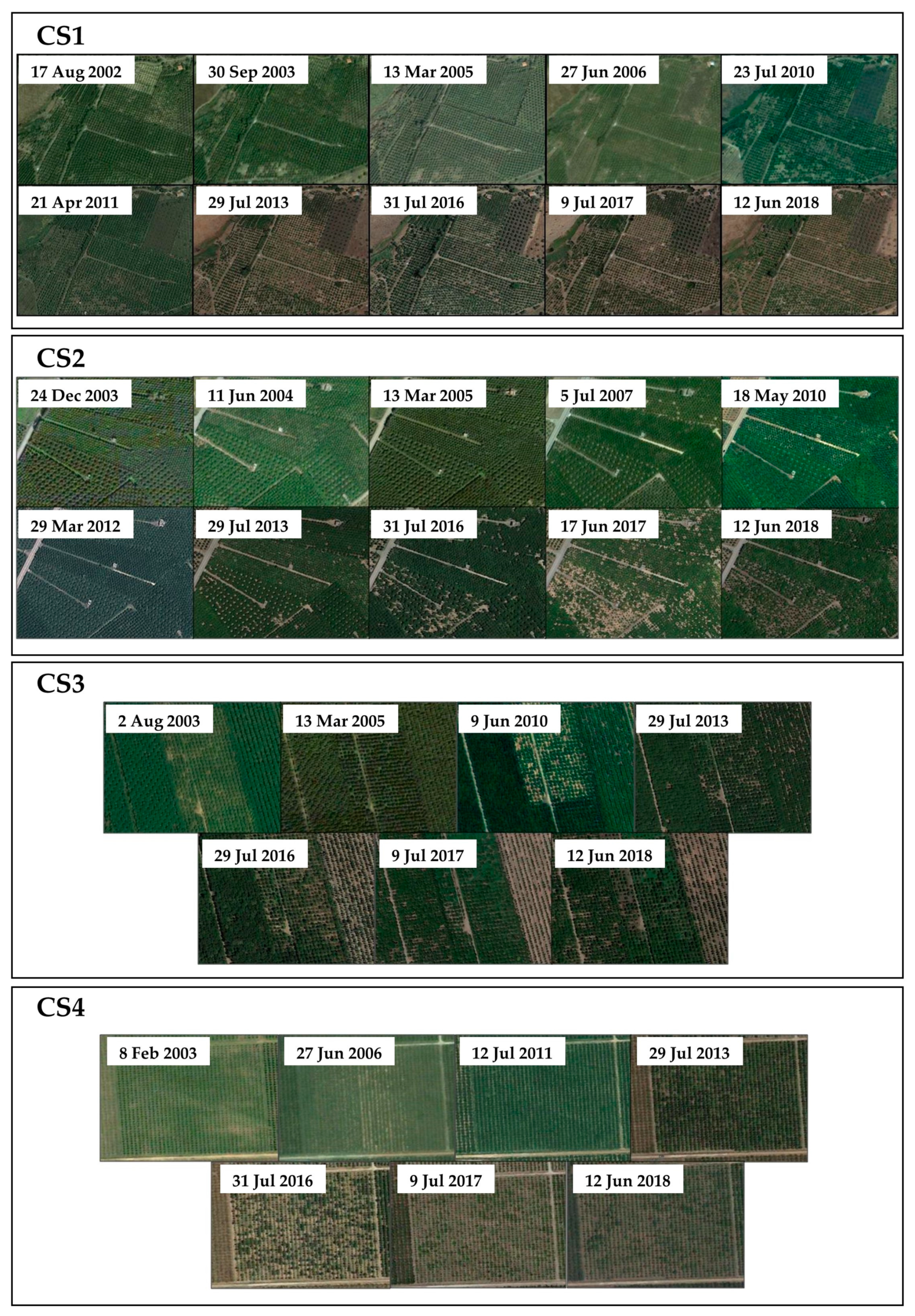
The preliminary evaluation of the evolution of the CTV and the timing of the related corrective actions (e.g., decline of the green, eradication of plants) during the MODIS 2001–2018 monitoring is based on the photointerpretation of the satellite images of Google Earth (https://earth.google.com/web/) and on interviews with farmers. To that purpose, the spatial resolution of the Google images was scaled at the MODIS pixel resolution (Figure 1).

2.2. MODIS Data

Free RS data were retrieved from MODIS sensor on board of the Terra satellite (https://modis.gsfc.nasa.gov/). Specifically, Terra-MODIS vegetation index (VI) product (MOD13Q1, Version 6 Level 3, [49]), generated every 16 days at 250 m of spatial resolution, was used for the time-series analyses. This product provides two primary vegetation layers: NDVI and Enhanced Vegetation Index (EVI). The MODIS algorithm chooses the best available pixel value from all the acquisitions from the 16-day period, on the basis of low cloud coverage, low view angle and the highest NDVI/EVI value. The main difference between the two VI layers is that EVI has improved sensitivity over high biomass areas, avoiding the problem of NDVI saturation [50]. However, in this study, NDVI was selected as the representative index of the vegetation dynamics because of the absence of NDVI saturation at the selected CSs (i.e., orange orchards).
In general, NDVI is representative of vegetation vigor [33], offering a valid tool for identifying/monitoring the vegetation status, mainly related to biotic and abiotic site conditions. It is calculated as follows:
N D V I = N I R R E D N I R + R E D ,
where NIR and RED are the reflectance values in the red and near-infrared bands of the electromagnetic spectrum, respectively.
In this study, NDVI time-series, referring to CS1–CS4, were analyzed in the period from 1 January 2001 to 31 December 2018. Data of the vegetation index were extracted and downloaded from the Global Subsets Tool [51]. This tool provides a summary of selected MODIS and VIIRS (Visible Infrared Imaging Radiometer Suite) products that can be freely used by the community for several applications (e.g., for validating models and remote-sensing products and for characterizing field sites) (https://modis.ornl.gov/cgi-bin/MODIS/global/subset.pl). The pixel selection (ID pixel, Table 1 and Figure 1) was defined using the geographic coordinates (latitude and longitude) of the center of the four selected CS. Eighteen years of NDVI time-series (23 images per year) were retrieved by Terra-MODIS for a total of 414 layers for each CS. Data quality was assessed by checking the VI Quality and Pixel Reliability indicators, that come together with the MOD13Q1 product.

2.3. Meteorological Data Clustering

Daily meteorological data, including solar radiation (Rs, MJ m−2), relative humidity (RH, minimum and maximum; %), air temperature (Tair, minimum, maximum, mean; °C), wind speed and direction (u2, m s−1 and WD, °) and rainfall (P, mm), were obtained by the Sistema Informativo Agrometeorologico Siciliano (SIAS). Specifically, the meteorological data were measured at two SIAS stations (in operation since 2002) located 6 km from CS1 (S234, 37.51°N, 14.85°E, 100 m a.s.l.) and about 2–8 km from CS2–CS4 (S292, 37.35°N, 14.91°E, 50 m a.s.l.). Daily meteorological data were averaged at 16-day intervals as the Terra-MODIS products used for deriving the NDVI time-series (see Section 2.2).
Figure 2 reports the 16-day meteorological data recorded at the weather stations S234 and S292 during the 2002–2018 period. No significant changes were observed in the main meteorological patterns during the reference period. In particular, the daily average values (± standard deviation) at 16-day intervals were 17.12 ± 6.56 MJ m−2 for Rs, 63.32 ± 9.63% for RH, 18.18 ± 6.25 °C Tair, 1.46 ± 0.38 m s−1 for u2 and 1.54 ± 2.21 mm for P.

2.4. TIMESAT Curving Fitting Method

The TIMESAT software (version 3.3), developed by [41], was used for generating smoothed NDVI time-series in the period 2001–2018 from Terra-MODIS satellite spectral measurements (see Section 2.2). The TIMESAT software is freely available at http://web.nateko.lu.se/timesat/timesat.asp and has a user-friendly graphical interface. It implements three CF methods: (i) the adaptive Savitzky–Golay filter that uses local polynomial functions for data fitting; and (ii) the asymmetric Gaussian and (iii) the double logistic model functions, both based on the least-squares methods, where data are fitted to non-linear model functions of different complexity. For these latter methods, the model functions are fitted to the data in intervals between maxima and minima of the time-series (t). The general form of the model functions is defined as:
f ( t ) = f ( t ;   c , x ) = c 1 + c 2 g ( t ; x )
where linear c parameters determine the base level (c1) and the amplitude (c2) for the seasons. The non-linear parameter x determines the shape of the basis function g (t; x) that in this study was considered as a double logistic filter [52], as reported in Equation (3):
g ( t ;   x 1 . x 4 ) = 1 1 + e x p   ( x 1 t x 2 ) 1 1 + e x p   ( x 3 t x 4 )
where the non-linear parameters x1 and x3 determine the position of the left and right inflection points for the season, respectively, whereas x2 and x4 determine the time period of increase and decrease (i.e., rate of change), respectively.
Firstly, a pre-processing phase was performed. It consists of the seasonality definition (e.g., fixed unimodal), which considers the growing seasons’ timings for the CSs under study (i.e., annual for citrus). No spikes and outliers were removed from the Terra-MODIS NDVI time-series at the CSs due to the high quality of the RS products used. Then, the season “start” and “end” were determined using the seasonal amplitude method, defined as the difference between the base level and the maximum NDVI value for each individual season. As reported in [53], the “start” occurs when the left part of the fitted curve has reached a specified fraction of the amplitude, counted from the base level. The “end” of the season is defined similarly, but for the right side of the curve. The details on the setting parameters used in this study are reported in Table 2.
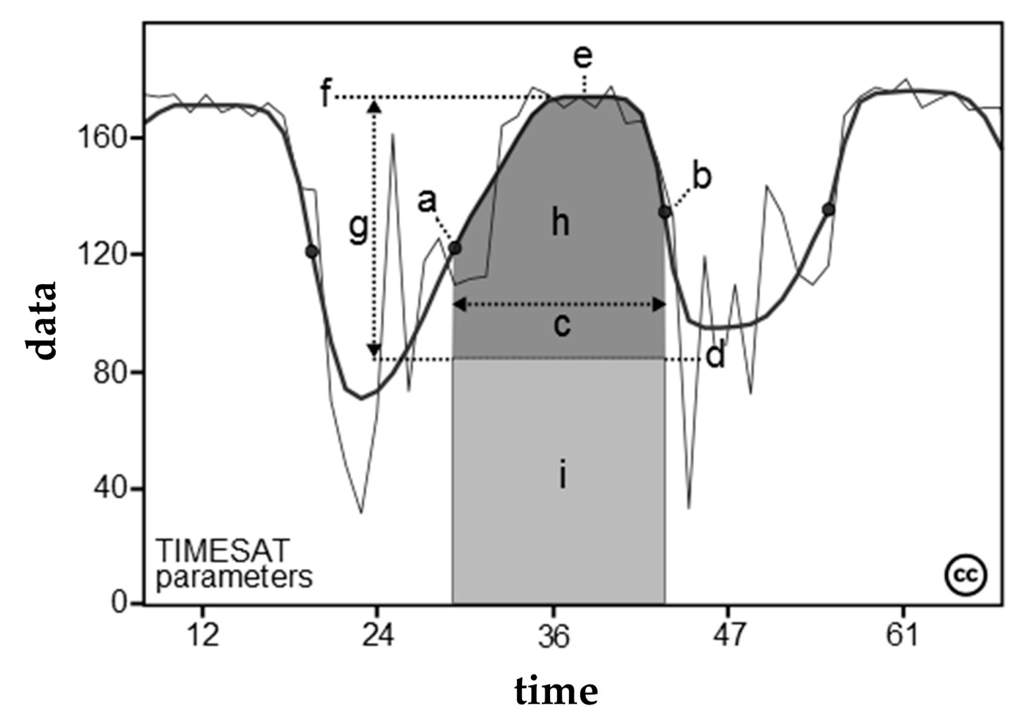
In order to exploit the information of the NDVI time-series, the derived phenological TIMESAT metrics were extracted and analyzed at the selected CSs during the reference period. Figure 3 shows the typical representation of the seasonality parameters [41] (as reported in Table 3).

2.5. Statistical Analysis

Linear regression models (Statistix analytical software, v. 9.0, Tallahassee, FL, USA) were adopted for analyzing the seasonal parameter trends. These trends were identified on the basis of the increasing/decreasing patterns (regression slope) and goodness-of-fit (coefficient of determination, R2). The significance of the trends was assessed for each seasonal parameter (Table 3) using the t-test at significance levels (p-value) of 0.05, 0.01 and 0.001, respectively.

3. Results

3.1. Case Studies Selection

The preliminary analysis of the Google Earth imagery provides useful insight for visualizing the CTV syndrome effects at the CSs (Figure 4). However, the limited temporal availability of the images does not permit a clear picture of the on-site CTV-related dynamics. In particular, CS1 (located 4 km in the southern-eastern direction from the first CTV epidemic focus) showed the presence of an irregular distribution of CTV symptomatic trees since 2002 (Figure 1). CS2–CS4 showed quite similar conditions, with the distinct identification of the following phases, corresponding to the epidemic evolution of CTV as a function of the distance from the first area of focus of the virus (Figure 1 and Figure 4): (i) growing phase (e.g., more evident in CS4 since trees were younger than in CS2 and CS3) together with the appearance of the symptomatic trees, and (ii) the adoption of corrective operations for the containment of CTV. In particular, CS2 (located 16 km in the south-western direction from the first CTV epidemic focus) exhibited the presence of the first symptomatic trees since 2007. At CS3 and CS4, the beginning of the CTV plant decline was observed starting from 2010 and 2013, respectively. These CSs were located 18 and 23 km from the CTV epidemic focus in the southern and southern-eastern directions, respectively.

3.2. Terra-MODIS NDVI Data

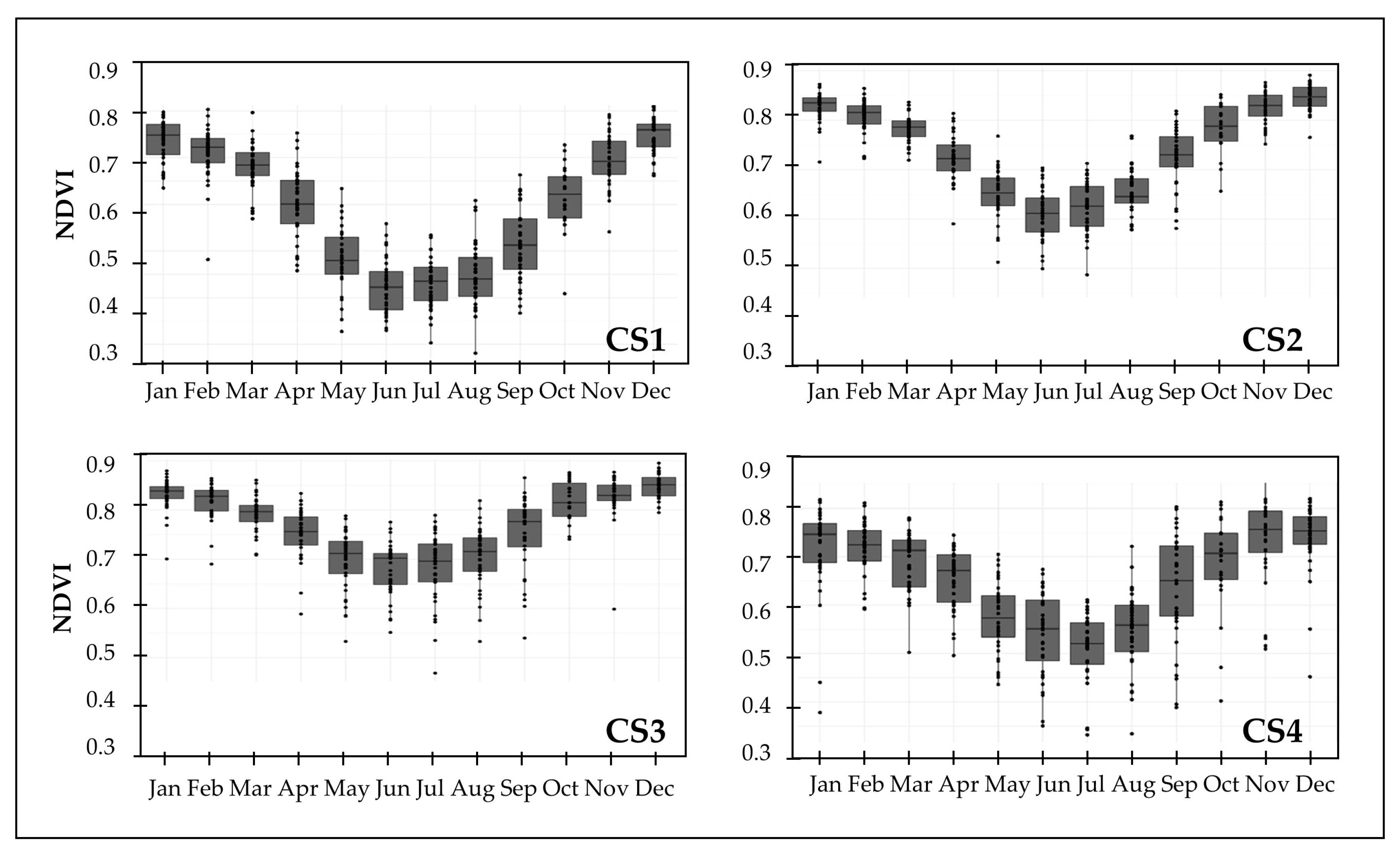
The analysis of the MOD13Q1 VI pixel quality and reliability indicators showed that the overall quality of the input data used here is classified as "good data" for 99% of the NDVI products. Figure 5 shows the temporal patterns of the Terra-MODIS NDVI data referring to CS1–CS4 during the 2001–2018 period. NDVI values ranged from 0.28 to 0.81 in CS1, from 0.43 to 0.89 in CS2, from 0.47 to 0.90 in CS3 and from 0.33 to 0.86 in CS4 (Figure 4). The highest mean (± standard deviation) NDVI values were observed at CS2 and CS3 (0.74 ± 0.09 and 0.76 ± 0.08, respectively), whereas lower NDVI values were detected at CS1 (0.59 ± 0.14) and CS4 (0.64 ± 0.11). Figure 6 shows the monthly NDVI box diagram for CS1–CS4 sites in the period of 2001–2018; this graph shows the minimum and maximum NDVI values found, respectively, in Summer (June–August) and in Autumn–Winter (January–February/October–December).

3.3. TIMESAT Fitting Curves

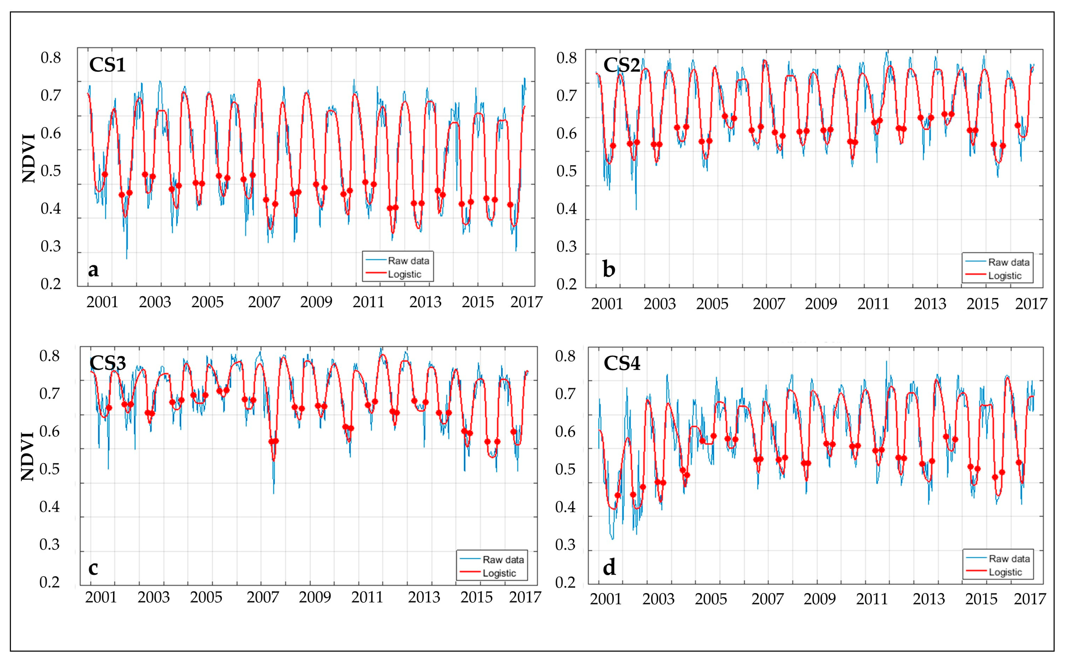
The time-series analysis was applied successfully to Terra-MODIS NDVI data of the different CSs. The fitted functions obtained by applying the double logistic filter CF method in TIMESAT (in red) to the original NDVI data (in blue) are shown in Figure 7. The “start” and the “end” of the growing seasons are marked with the red filled circles. Generally, the fitting curves reproduced the NDVI data quite well (Figure 7) due to their high quality, typical of clear sky conditions (i.e., absence of spikes of outliers).

3.4. Seasonal Parameters from NDVI Time-Series

The TIMESAT seasonal parameters extracted in CS1–CS4 were useful for depicting the site-specific dynamics that occurred during the reference period (2001–2018) (Figure 8, Figure 9, Figure 10 and Figure 11).
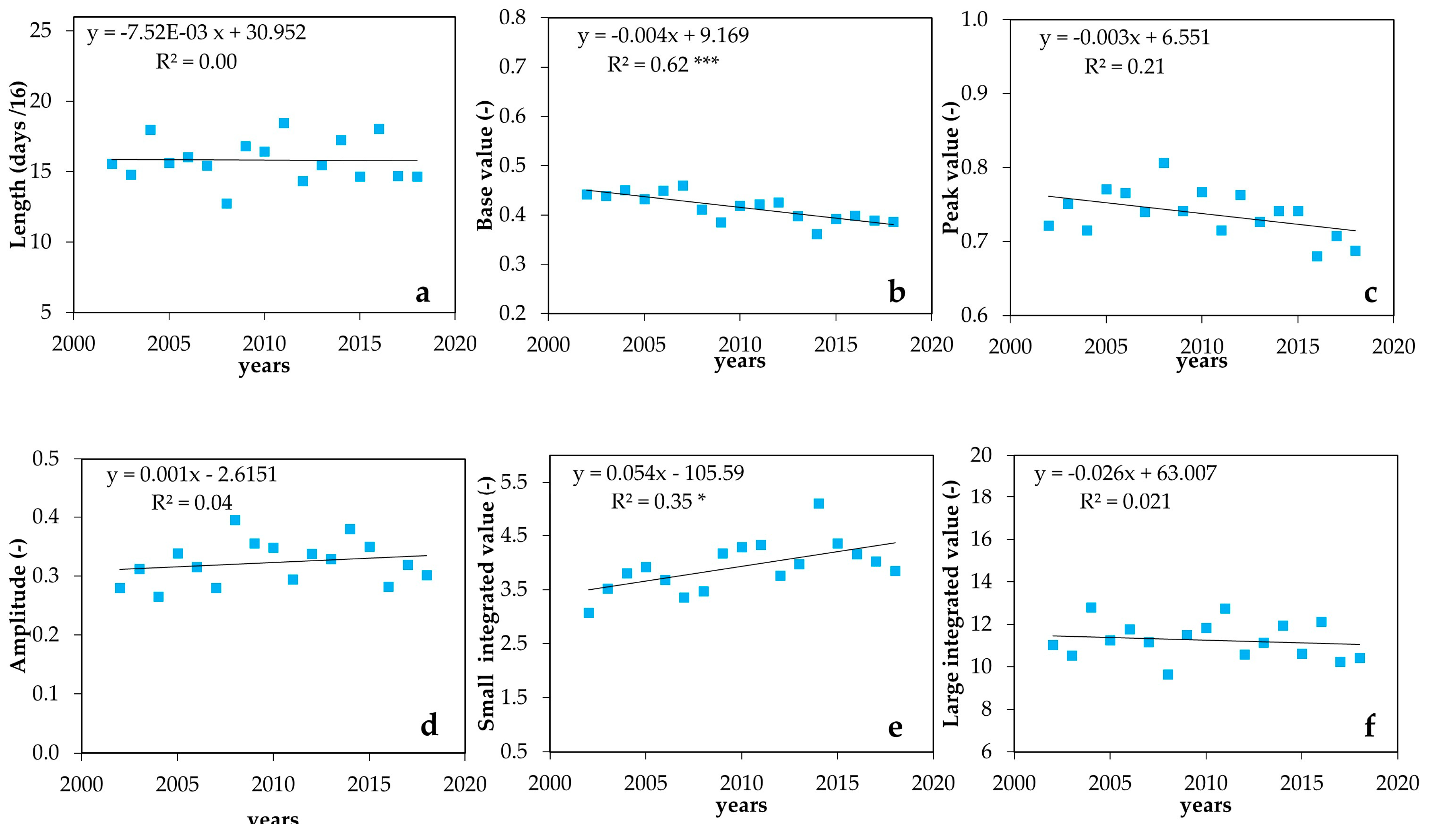
In particular, in CS1, near-stable trends of the seasonal parameters were observed i 2001–2018, with slopes ranging from −0.03 to 0.05 and low values of R2 for all parameters (R2 between 0 and 0.35, even with the significant trend for “Small integrated value”, p < 0.05) except for the “Base value”, which reached an R2 of 0.62 (p < 0.001) (Figure 8).
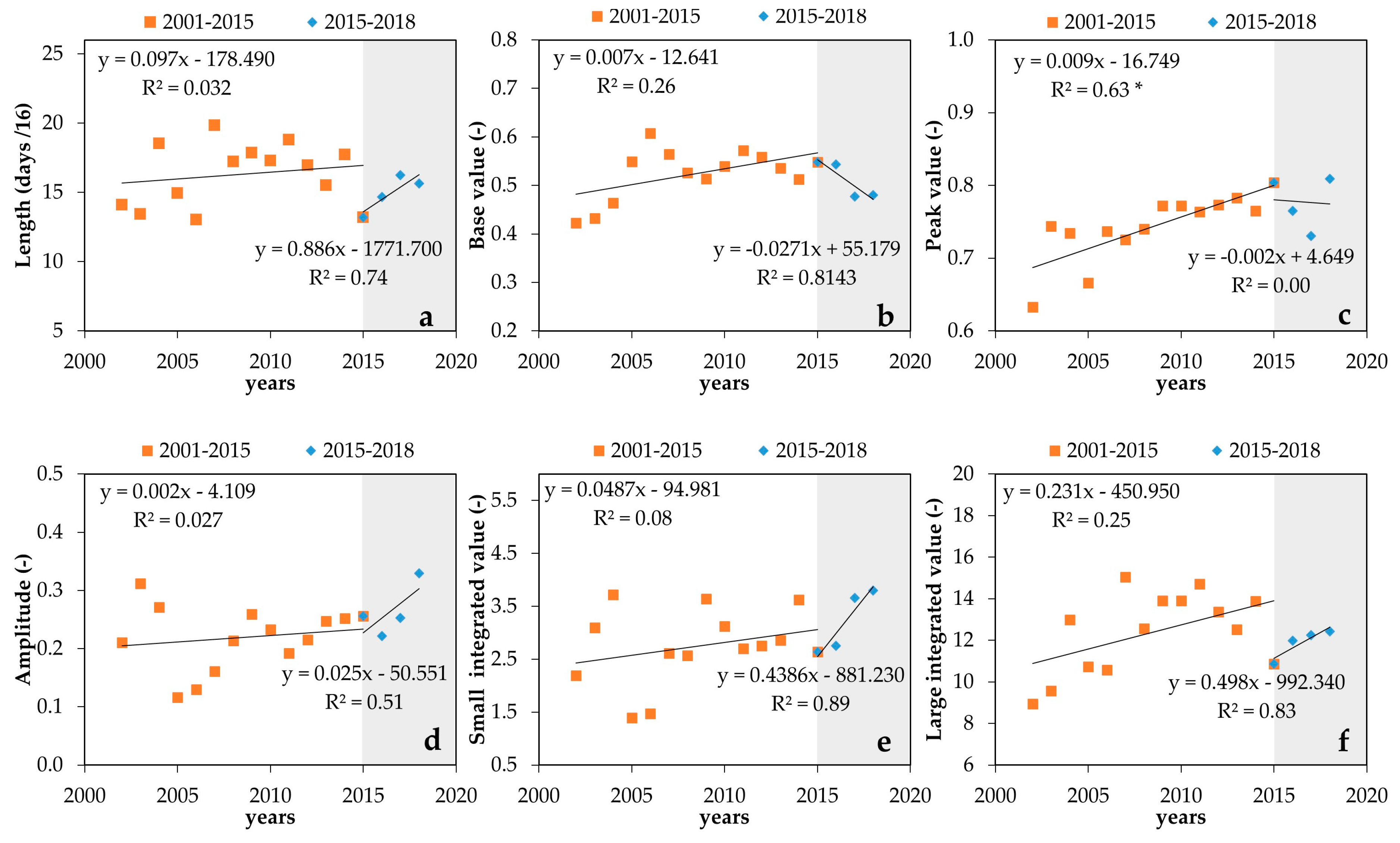
In contrast to CS1, two different phases were identified in CS2–CS4 on the basis of the photo-interpretation analysis (Figure 9, Figure 10 and Figure 11). Specifically, in CS2, the parameter that better identified the first phase was the “Base value” (R2 of 0.48, p < 0.01), whereas in CS3 and CS4, this phase was well represented by the “Peak value” (R2 of 0.37 and 0.63, respectively, p < 0.05). At CS3, “Amplitude” and “Small integrated value” also contributed in representing the first phase (R2 of 0.33 and 0.36, respectively, p < 0.05).
Regarding the second phase, the “Base value” (R2 of 0.58) and the “Peak value” (R2 of 0.54) represented better this trend in CS2, even with no significance trends (p < 0.05). In CS3, this second phase was more clearly observed than in CS2, with the “Base value” and “Peak value” (R2 of 0.88 and 0.93, respectively) being the most representative parameters (p < 0.05 and 0.01). The performance obtained from TIMESAT in CS4 was different, with the parameters explaining the trend being the “Length” (R2 of 0.74), “Base value” (R2 of 0.81), “Small and Large seasonal integral values” (R2 of 0.86 and 0.83, respectively); those parameters provided the highest R2 values, even with no significant trends.
When analyzing individually each seasonal parameter, it was observed that, in general, the trends observed in all the CSs were quite similar (Figure 8, Figure 9, Figure 10 and Figure 11). The “Length” parameter presented a positive slope term that ranged from 0.10 to 0.19 and from 0.04 to 0.89 in the first and second phases, respectively. The “Base value” exhibited a positive slope term in the first phase (ranging from 0.00 to 0.01 in all CS), whereas the patterns are inverted in the second phase, showing negative slope terms (−0.03 to −0.02). “Peak value” showed a trend similar to “Base value”, with positive slopes in the first phase (0.00–0.01) and negative slopes in the second phase (−0.01 to 0.00). Regarding the “Amplitude” and “Small integrated value”, in CS3 and CS4 they exhibited positive slope values in the first phase (ranging from 0.00 to 0.01 and from 0.05 to 0.10, for “Amplitude” and “Small integrated value”, respectively). Conversely, in the first phase in CS2, these parameters had negatives slopes (ranging from −0.02 to −0.00). Nevertheless, the behavior of “Amplitude” and “Small integrated value” in the second phase was similar in CS2–CS4, with slopes ranging from 0.01–0.02 and from 0.12–0.44 for “Amplitude” and “Small integrated value”, respectively. The “Large integrated value” presented positive slopes in the first phase (0.15–0.23), whereas it changed the sign in the second phase (slope terms of −0.14 and −0.23 at CS2 and CS3, respectively), except for CS4, where a positive slope value was observed (0.50; Figure 11).
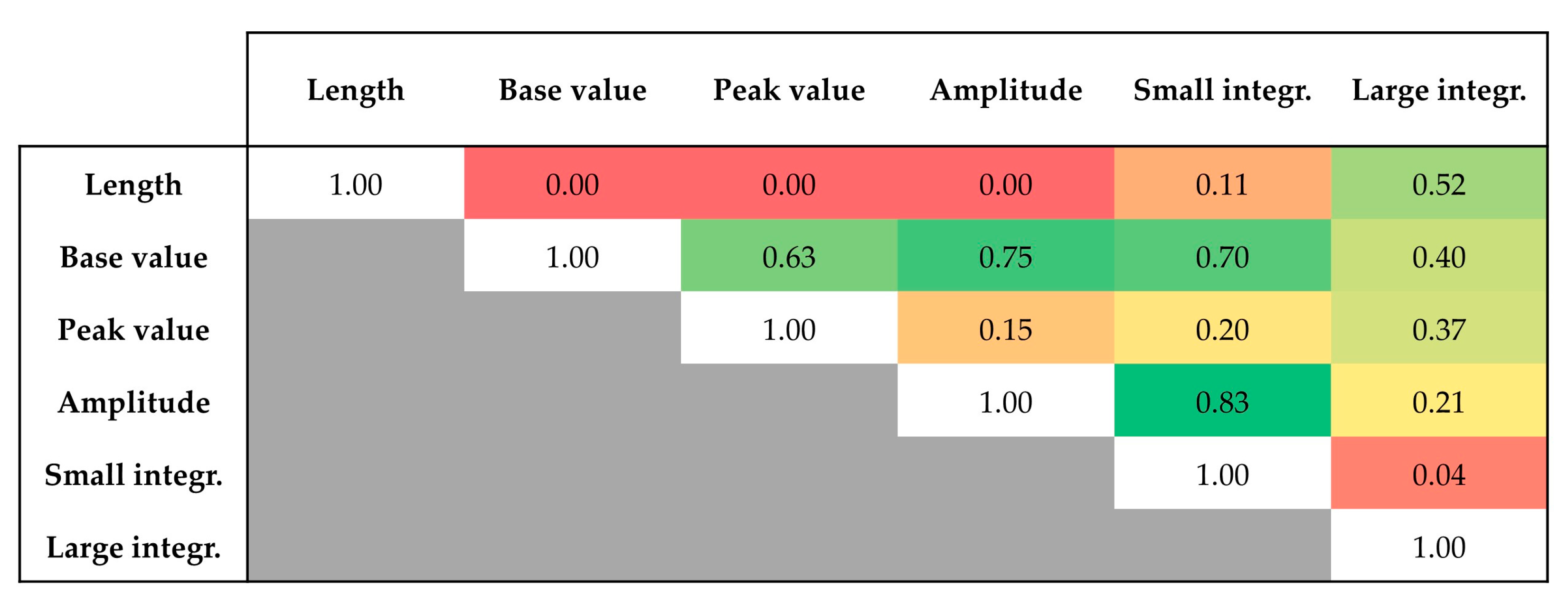
By analyzing the inter-seasonality parameter relationship in terms of R2, it can be observed that, in general, good relationships were observed between “Length” and “Large integrated value” (R2 = 0.52) and between “Amplitude” and “Small integrated value” (R2 = 0.83) (Figure 12). In addition, the “Base value” showed good relationships with “Peak value”, “Small integrated value” and “Amplitude”, with R2 values of 0.63, 0.70 and 0.75, respectively. The relationships between the other parameters were quite poor with R2 values lower than 0.41.

4. Discussion

TIMESAT software and MODIS products have been widely used in the agriculture context. Specifically, [54] explored their potential for accurately deriving crop phenological metrics in comparison with ground-observed vegetation green-up dates. Additionally, the suitability of TIMESAT with different MODIS-derived VI time series has been assessed for large area vegetation dynamic monitoring over arid and semi-arid lands [55]. TIMESAT has been also used to evaluate the scaling effects on spring phenology detections using MODIS data at multiple spatial resolutions [56]. In addition, [57,58,59] highlighted the strengths of the TIMESAT approach for mapping crop phenological stages and crop-calendar events, and for crop classification. Despite these promising applications, the main weakness of TIMESAT implementation is related to the correct choice of the CF method capable of providing the most robust description of the seasonal dynamics [58,59,60]. Other limitations are due to the influence of noise level of data input on CF technique performance [60,61] and the presence of sample impurity and landscape heterogeneities that can largely affect the classification accuracy [59]. Nowadays, although several authors have compared different CF methods for identifying vegetation features changes through VI metrics, no consensus has been reached in the election of the best CF method (e.g., [22,24,56,60,61,62]). In general, authors corroborated that the choice of the most suitable CF method (and filtering parameters) depends on the quality of the input data and has to be assessed case-by-case by inspecting how well the CF functions match the row data for preserving the signal integrity [63].
In this study, the double-filter CF method was selected for analyzing the main seasonal parameters of areas affected by CTV in Sicily, with this choice being supported by the excellent quality of the Terra-MODIS NDVI data used as inputs (Figure 5, Figure 6 and Figure 7). Specifically, no spikes or outliers were detected in the NDVI time-series, which were quite robust, consisting of 18 years of continuous data with 16-day temporal resolution. Even though multiple definitions of seasonality parameters and ways for extracting these parameters are reported in RS literature [53], the importance of the seasonal parameters lies in the possibility to describe the temporal changes in the vegetation cover resulting from abiotic or biotic changes (climatic or land use or disease).
The time-series of NDVI at the different CSs (Figure 5 and Figure 6) have shown a typical annual pattern deriving from the sum of two contributions: (i) the fairly stable vegetation dynamic of citrus trees and (ii) the presence of typical conditions of grassed soil [64,65,66,67]. It can be assumed, given that the ground cover plays a role of constant "background" every year, that the dynamics of the seasonal NDVI parameters are mainly linked to the presence of citrus groves. In addition, some of the seasonal parameters analyzed (e.g., "Base value", defined as the average of the minimum left and right NDVI values within a season) are independent of the presence of ground cover since they refer to summer periods, when the soil is generally bare due to weed control. Furthermore, the age of trees can play a crucial role in specific seasonal parameter trends. This effect is more evident when the trees are not subject to any management of the size of the canopy (for example, some rain-fed olive groves with large planting structures). However, the size of the crown of citrus groves is commonly managed by pruning, especially in the Sicilian context, where the citrus systems are maintained in a fairly stable size. Therefore, despite the wide age range of the citrus groves examined in this study (which vary from 25 to 60 years, Table 1), and given that the canopy size is kept almost constant, the main differences in the seasonal parameters of NDVI depend on the citrus groves pathology. This is also supported by similar time patterns for the main meteorological variables observed in the two stations located close to the CSs during the reference period (Figure 1 and Figure 2). This allows us to imagine that the observed trends for NDVI are quite independent of the variability of meteorological parameters.
Results derived from TIMESAT analysis reflected a stable pattern of the seasonal parameters in CS1, which can be related to the in situ conditions influenced both by the CTV effects on plants and by the adoption of spotted mitigation actions such as eradication of infected plants and replanting with trees grafted on tolerant rootstocks in order to prevent economic damages since 2002 (Figure 4). This stability also reflected the low rate of plant growing in CS1 as a consequence of the tree age (Table 1), indicating that the plant growing stage has been reduced. Nevertheless, the temporal trends of the seasonal parameters in CS2–CS4 allowed recognizing two different phases (Figure 9, Figure 10 and Figure 11), accordingly identified by the Google Earth imagery analysis (Figure 4). The first phase (observed in the period 2001–2014 in CS2 and CS3 and in the period 2001–2015 in CS4) corresponded to the citrus growing period in combination with the occurrence of the CTV epidemic effects. Therefore, this phase was characterized by a slight increase of all seasonality parameters with the exception of “Amplitude” and “Small integrated value” in CS2, which experienced a decrease, probably because in this site CTV has been present for longer without being countered by corrective measures. The second phase (observed in the period of 2014–2018 in C2 and CS3 and in the period of 2015–2018 in CS4) was characterized by the corrective measures applied by the growers for facing CTV (such as eradication and trees replanting on CTV-tolerant rootstocks) (see the grey areas in Figure 9, Figure 10 and Figure 11). In this phase “Length”, “Amplitude” and “Small integrated value” experienced increasing patterns in CS2–CS4, whereas “Base value”, “Peak value” and “Large integrated value” showed a decreasing trend with the exception of “Large integrated value” in CS4. At this site, the intensive corrective actions taken since 2015 by the grower strongly modified the NDVI signals, with an abrupt increase of the “Length” and “Amplitude” (positive slopes), resulting in a more evident increase of “Small integrated value” and “Large integrated value”.
In the first phase, a number of parameters were able to accurately describe the vegetation dynamics at the different CS. Specifically, in CS1 (Figure 4 and Figure 8), the contemporary occurrence of CTV with mitigations actions was observed in the “Base value”, whereas in CS2–CS4, site-specific patterns in the seasonality parameters were distinguished within the first phase due to tristeza severity. These patterns are more related to the range of variations (minimum and maximum values) of the seasonal parameters (e.g., “Base value”, “Peak value”, “Amplitude” and “Small integrated value”), than to their “Length”. For example, the CTV epidemic effects were better identified once more by “Base value” in CS2 (i.e., which experienced CTV syndrome since 2007) than in CS3 and CS4 (i.e., which experienced CTV since 2010 and 2013 ), by the “Peak value” in CS3 and CS4, and by this latter parameter plus “Amplitude” and “Small integrated value” in CS3.
Regarding the second phase, the “Base value” and “Peak value” were recognized as the most representative seasonal parameters of the site-specific conditions in CS3, giving a picture of the timing of CTV-corrective actions and the epidemic evolution.
However, care should be taken in analyzing the linear relationship of the seasonal parameters, which in some cases showed a low magnitude of the R2 values. In this sense, future research must tend to couple linear and non-linear trends and to analyze seasonal variations, cyclical variations, random or irregular patterns.
In addition, the “Base value” showed a well-defined increasing trend in CS2–CS4 (Figure 9, Figure 10 and Figure 11), as a function of the changes in NDVI due to the adoption of CTV-corrective actions, even without a significant trend due to the limited numbers of years considered in the second phase. More specifically, these actions were more intense in CS4, followed by CS3 and CS2, as can be observed by the slope terms in Figure 9, Figure 10 and Figure 11. Therefore, as observed in Figure 8, Figure 9, Figure 10 and Figure 11, the “Base value” helps to provide information on the evolution of the areas affected by the CTV.
Furthermore, the matrix in Figure 12 shows high R2 values between the "Base value" and most of the other parameters, suggesting that the analysis of the seasonal parameters for monitoring the areas affected by CTV can be limited to the evaluation of this parameter.
This study contributes to corroborate the significant use of RS technologies in the phytopathology field of application. In fact, RS applications have recently already demonstrated their promising ability for describing and monitoring plant diseases with respect to field- and laboratory-based analyses (e.g., [68,69]). The main limitation of these latter approaches (e.g., including visual inspection for symptoms at early stages and spectroscopic and imaging techniques) is that they are time-consuming, i.e., needing a large number of samples, expensive [70] and not standardized because they are influenced by the observer’s expertise. The main advantage of using RS technologies is their cheapness and the ability to provide a large-scale detector for pathogen control [38]. The potential use of time-series RS procedures can be exploited for being adapted in phytopathology studies and being used as a monitoring system of long-term changes [71].
CTV is one of the most complex pathosystems known in plant virology [72]. This complexity is determined by some key factors: the quasispecies nature of viruses, which makes them particularly prone to the continuous evolution of populations of variants under selective pressure operated by the genome of the hosts and the climatic conditions; the vastness of the genetic patrimony of rutaceous hosts; the use of rootstocks with different susceptibility, which determines another important factor of deep interaction with the virus; the quite vast climatic range as well as the soil conditions of citrus growing areas. The number and diversity of these involved factors leads to a very large plethora of disease phenotypes being related to the pathogen. In this context, the effects of CTV on yield are difficult to estimate also due to the fact that, in most phenotypes, the plants died within a few years, as in the case of the CTV epidemic in Sicily, where the syndrome had a rapid evolution with the death of the plants in about 2 years after the infection. In 2002, it was estimated that CTV had caused the death of about 80 million citrus trees worldwide, about half of which were in Spain [73]. When the main symptoms of yellowing foliage or plant decline are visible, the pathogenic process is already at an advanced stage; for this reason, the development of stress detection systems based on RS or proximal sensing techniques is desirable [74,75] because it would allow the early interception of viral infection and the application of more effective containment methods (e.g., elimination of inoculation sources).
The approach developed in this study is valid to be transferred to regional agencies involved in and/or in charge of the management of devastating plant diseases, especially if it is integrated with ground-based early detection methods or high-resolution thermal and hyperspectral imagery acquired by airborne and/or unmanned aerial vehicles (UAV), for the early detection and quantification of plant diseases, (i.e., Xylella fastidiosa [76], Verticillium dahliae infections in Olea europaea L. [77], red leaf blotch in Prunus amigdalus [78]), especially in the case of quarantine plant pathogens requiring complex control schemes that must be readily adaptable to the evolution of epidemics. Furthermore, the application carried out under these heterogeneous conditions of citrus crops can allow the methodology for large-scale interventions and epidemic management programs to be exported.

5. Conclusions

The adoption of the RS approach described for the characterization of long-term changes in NDVI Terra-MODIS data was performed with the aim of bridging the gap between the temporal distribution of CTV diseases and the recognition of corrective mitigation actions implemented autonomously by growers.
This study outlined the history of the tristeza epidemic in Sicily and showed how the management choices were ineffective because they were not coordinated at the regional level. In fact, the legislative gap of about 14 years between the first version of the Italian Ministerial Decree for compulsory control of the CTV (1996) and the current version, implemented only in 2014, has reinforced the difficulty of farmers in implementing effective operational choices. As a result, fragmentation of interventions is observed, which, if analyzed from an economic point of view, outlines a picture of avoidable economic losses.
The main results obtained from the study are the following:
  • The Terra-MODIS products represented a valuable data source for the implementation of long-term time series approaches and for the support of phytopathological studies, the limitation of the spatial resolution being largely compensated by their high temporal resolution and the availability of images for long time intervals;
  • The Terra-MODIS time series approach has proven to be reliable for identifying the specific phenological phases of citrus groves linked to the evolution of CTV, with reference to conditions prior to and subsequent to the implementation of corrective measures by farmers;
  • Considering TIMESAT statistics analyzed, the “Base value” was identified as a representative proxy for identifying the timing of corrective actions to contain the CTV.
To conclude, it is necessary to underline that the management of severe epidemic events cannot be left solely to individual farmers, but instead, it needs coordinated short-, medium- and long-term interventions. The remote-sensed-based time series analysis proposed in this study is economically advantageous and, if used at the level of territories or regions, it would therefore be useful both in the forecasting phase of the epidemic trend and in the phase of the definition of management interventions.

Author Contributions

All authors have contributed with equal effort to the realization of the study, as follows: Conceptualization, D.V., S.C., J.M.R.-C. and M.T.; data curation, D.V. and J.M.R.-C.; funding acquisition, S.C.; investigation, D.V., S.C. and J.M.R.-C.; methodology, D.V., S.C. and J.M.R.-C.; supervision, S.C. and M.T.; writing—original draft, D.V., S.C., J.M.R.-C. and M.T. All authors have read and agreed to the published version of the manuscript.

Funding

This research was funded by “Fondi di ateneo 2020–2022, Università di Catania, linea Open Access”.

Acknowledgments

The authors wish to thank Alberto Sacco for acquiring the field sites information.

Conflicts of Interest

The authors declare no conflict of interest. The funders had no role in the design of the study; in the collection, analyses, or interpretation of data; in the writing of the manuscript, or in the decision to publish the results.

References

  1. Martínez, B.; Gilabert, M.A. Vegetation dynamics from NDVI time series analysis using the wavelet transform. Remote Sens. Environ. 2009, 113, 1823–1842. [Google Scholar] [CrossRef]
  2. Reddy, D.S.; Prasad, P.R.C. Prediction of vegetation dynamics using NDVI time series data and LSTM. Model. Earth Syst. Environ. 2018, 4, 409–419. [Google Scholar] [CrossRef]
  3. Lausch, A.; Bastian, O.; Klotz, S.; Leitão, P.J.; Jung, A.; Rocchini, D.; Schaepman, M.E.; Skidmore, A.; Tischendorf, L.; Knapp, S. Understanding and assessing vegetation health by in situ species and remote-sensing approaches. Methods Ecol. Evol. 2018, 9, 1799–1809. [Google Scholar] [CrossRef]
  4. D’onghia, A.M.; Santoro, F.; Gualano, S. The application of remote sensing in the official monitoring of Citrus tristeza virus and Xylella fastidiosa. In Proceedings of the Perspectives on the Use of Remote Sensing in Plant Health Scientific Colloquium organised by EPPO & EUPHRESCO UNESCO, Paris, France, 27 September 2018; p. 7. [Google Scholar]
  5. Abu-Khalaf, N. Sensing tomato’s pathogen using Visible/Near infrared (VIS/NIR) spectroscopy and multivariate data analysis (MVDA). Palest. Tech. Univ. Res. J. 2015, 3, 12–22. [Google Scholar]
  6. Lorente, D.; Escandell-Montero, P.; Cubero, S.; Gómez-Sanchis, J.; Blasco, J. Visible–NIR reflectance spectroscopy and manifold learning methods applied to the detection of fungal infections on citrus fruit. J. Food Eng. 2015, 163, 17–24. [Google Scholar] [CrossRef]
  7. Sankaran, S.; Maja, J.M.; Buchanon, S.; Ehsani, R. Huanglongbing (Citrus Greening) Detection Using Visible, Near Infrared and Thermal Imaging Techniques. Sensors 2013, 13, 2117–2130. [Google Scholar] [CrossRef] [Green Version]
  8. Krezhova, D.D.; Iliev, I.T.; Hristova, D.P.; Yanev, T.K. Spectral remote sensing measurements for detection of viral infections in tobacco plants (Nicotiana tabacum L.). Fund. Space Res. 2009, 2009, 43–46. [Google Scholar]
  9. Naidu, R.A.; Perry, E.M.; Pierce, F.J.; Mekuria, T. The potential of spectral reflectance technique for the detection of Grapevine leafroll-associated virus-3 in two red-berried wine grape cultivars. Comput. Electron. Agric. 2009, 66, 38–45. [Google Scholar] [CrossRef]
  10. Grisham, M.; Johnson, R.M.; Zimba, P.V. Detecting Sugarcane yellow leaf virus infection in asymptomatic leaves with hyperspectral remote sensing and associated leaf pigment changes. J. Virol. Methods 2010, 167, 140–145. [Google Scholar] [CrossRef]
  11. Parnell, S.; Bosch, F.V.D.; Gottwald, T.; Gilligan, C.A. Surveillance to Inform Control of Emerging Plant Diseases: An Epidemiological Perspective. Annu. Rev. Phytopathol. 2017, 55, 591–610. [Google Scholar] [CrossRef] [Green Version]
  12. Mahlein, A.-K.; Kuska, M.T.; Behmann, J.; Polder, G.; Walter, A. Hyperspectral Sensors and Imaging Technologies in Phytopathology: State of the Art. Annu. Rev. Phytopathol. 2018, 56, 535–558. [Google Scholar] [CrossRef] [PubMed]
  13. Afonso, A.M.; Guerra, R.; Cavaco, A.M.; Pinto, P.I.; Andrade, A.; Duarte, A.; Power, D.M.; Marques, N.T. Identification of asymptomatic plants infected with Citrus tristeza virus from a time series of leaf spectral characteristics. Comput. Electron. Agric. 2017, 141, 340–350. [Google Scholar] [CrossRef]
  14. Bruzzone, L.; Smits, P.; Tilton, J. Foreword special issue on analysis of multitemporal remote sensing images. IEEE Trans. Geosci. Remote Sens. 2003, 41, 2419–2422. [Google Scholar] [CrossRef]
  15. Coppin, P.; Jonckheere, I.; Nackaerts, K.; Muys, B.; Lambin, E. Review ArticleDigital change detection methods in natural ecosystem monitoring: A review. Int. J. Remote Sens. 2004, 25, 1565–1596. [Google Scholar] [CrossRef]
  16. Lambin, E.; Linderman, M. Time series of remote sensing data for land change science. IEEE Trans. Geosci. Remote Sens. 2006, 44, 1926–1928. [Google Scholar] [CrossRef]
  17. Ramírez-Cuesta, J.M.; Rodríguez-Santalla, I.; Gracia, F.J.; Sánchez, M.J.; Barrio-Parra, F. Application of change detection techniques in geomorphological evolution of coastal areas. Example: Mouth of the River Ebro (period 1957–2013). Appl. Geogr. 2016, 75, 12–27. [Google Scholar] [CrossRef]
  18. Sheoran, S.; Mittal, N.; Gelbukh, A. Analysis on application of swarm-based techniques in processing remote sensed data. Earth Sci. Inform. 2019, 13, 97–113. [Google Scholar] [CrossRef]
  19. Iounousse, J.; Er-Raki, S.; El Motassadeq, A.; Chehouani, H. Using an unsupervised approach of Probabilistic Neural Network (PNN) for land use classification from multitemporal satellite images. Appl. Soft Comput. 2015, 30, 1–13. [Google Scholar] [CrossRef]
  20. Yun, L.; Qing-Wei, P.; Jian-Cheng, Y.; Tang, Y.-L. Identification of tea based on CARS-SWR variable optimization of visible/near-infrared spectrum. J. Sci. Food Agric. 2019, 100, 371–375. [Google Scholar] [CrossRef]
  21. Venkata Subramanian, N.; Saravanan, N.; Bhuvaneswari, S. K-means based probabilistic neural network (KPNN) for designing physical machine–classifier. Int. J. Innov. Technol. Explor. Eng. 2019, 9, 800–804. [Google Scholar]
  22. Hall-Beyer, M. Comparison of single-year and multiyear ndvi time series principal components in cold temperate biomes. IEEE Trans. Geosci. Remote Sens. 2003, 41, 2568–2574. [Google Scholar] [CrossRef] [Green Version]
  23. Bradley, B.A.; Jacob, R.W.; Hermance, J.F.; Mustard, J.F. A curve fitting procedure to derive inter-annual phenologies from time series of noisy satellite NDVI data. Remote Sens. Environ. 2007, 106, 137–145. [Google Scholar] [CrossRef]
  24. Galford, G.L.; Mustard, J.F.; Melillo, J.; Gendrin, A.; Cerri, C.E.P.; Cerri, C.E.P. Wavelet analysis of MODIS time series to detect expansion and intensification of row-crop agriculture in Brazil. Remote Sens. Environ. 2008, 112, 576–587. [Google Scholar] [CrossRef]
  25. Zhang, X.; Friedl, M.A.; Schaaf, C.; Strahler, A.H.; Hodges, J.C.; Gao, F.; Reed, B.C.; Huete, A. Monitoring vegetation phenology using MODIS. Remote Sens. Environ. 2003, 84, 471–475. [Google Scholar] [CrossRef]
  26. Jönsson, P.; Eklundh, L. Seasonality extraction by function fitting to time-series of satellite sensor data. IEEE Trans. Geosci. Remote Sens. 2002, 40, 1824–1832. [Google Scholar] [CrossRef]
  27. Reed, B.C.; Brown, J.F.; Vanderzee, D.; Loveland, T.R.; Merchant, J.W.; Ohlen, D.O. Measuring phenological variability from satellite imagery. J. Veg. Sci. 1994, 5, 703–714. [Google Scholar] [CrossRef]
  28. Ruimy, A.; Saugier, B.; Dedieu, G. TURC: A diagnostic model of continental gross primary productivity and net primary productivity. Glob. Biogeochem. Cycles 1996, 10, 269–285. [Google Scholar] [CrossRef]
  29. Malmström, C.M.; Thompson, M.V.; Juday, G.P.; Los, S.; Randerson, J.T.; Field, C.B. Interannual variation in global-scale net primary production: Testing model estimates. Glob. Biogeochem. Cycles 1997, 11, 367–392. [Google Scholar] [CrossRef] [Green Version]
  30. Sellers, P.J.; Tucker, C.J.; Collatz, G.J.; Los, S.O.; Justice, C.O.; Dazlich, D.A.; Randall, D.A. A global 1° by 1° NDVI data set for climate studies. Part 2: The generation of global fields of terrestrial biophysical parameters from the NDVI. Int. J. Remote Sens. 1994, 15, 3519–3545. [Google Scholar] [CrossRef]
  31. Wylie, B.K. Calibration of remotely sensed, coarse resolution NDVI to CO2 fluxes in a sagebrush–steppe ecosystem. Remote Sens. Environ. 2003, 85, 243–255. [Google Scholar] [CrossRef]
  32. Jeevalakshmi, D.; Reddy, S.N.; Manikiam, B. Land cover classification based on NDVI using LANDSAT8 time series: A case study Tirupati region. In Proceedings of the International Conference on Communication and Signal Processing (ICCSP), Melmaruvathur, India, 6–8 April 2016; IEEE: New York, NY, USA, 2016; pp. 1332–1335. [Google Scholar] [CrossRef]
  33. Rouse, J.W.; Haas, R.H.; Schell, J.A.; Deering, D.W. Monitoring vegetation system in the great plains with ERTS. In Proceedings of the Third ERST Symposium, Washington, DC, USA, 10–14 December 1973; NASA SP-351. Volume 1, pp. 309–317. [Google Scholar]
  34. Wang, R.; Gamon, J.A.; Montgomery, R.A.; Townsend, P.A.; Zygielbaum, A.I.; Bitan, K.; Tilman, D.; Cavender-Bares, J. Seasonal Variation in the NDVI–Species Richness Relationship in a Prairie Grassland Experiment (Cedar Creek). Remote Sens. 2016, 8, 128. [Google Scholar] [CrossRef] [Green Version]
  35. Lyu, H.; Lu, H.; Mou, L. Learning a Transferable Change Rule from a Recurrent Neural Network for Land Cover Change Detection. Remote Sens. 2016, 8, 506. [Google Scholar] [CrossRef] [Green Version]
  36. Shimabukuro, Y.E.; Beuchle, R.; Grecchi, R.C.; Achard, F. Assessment of forest degradation in Brazilian Amazon due to selective logging and fires using time series of fraction images derived from Landsat ETM+ images. Remote Sens. Lett. 2014, 5, 773–782. [Google Scholar] [CrossRef]
  37. Verbesselt, J.; Hyndman, R.J.; Newnham, G.; Culvenor, D. Detecting trend and seasonal changes in satellite image time series. Remote Sens. Environ. 2010, 114, 106–115. [Google Scholar] [CrossRef]
  38. Forkel, M.; Carvalhais, N.; Verbesselt, J.; Mahecha, M.D.; Neigh, C.S.; Reichstein, M. Trend Change Detection in NDVI Time Series: Effects of Inter-Annual Variability and Methodology. Remote Sens. 2013, 5, 2113–2144. [Google Scholar] [CrossRef] [Green Version]
  39. Filippa, G.; Cremonese, E.; Migliavacca, M.; Galvagno, M.; Forkel, M.; Wingate, L.; Tomelleri, E.; Morra di Cella, U.; Richardson, A.D. Phenopix: AR package for image-based vegetation phenology. Agric. For. Meteorol. 2016, 220, 141–150. [Google Scholar] [CrossRef] [Green Version]
  40. Estay, S.A.; Chávez, R.O. npphen: An R-package for non-parametric reconstruction of vegetation phenology and anomaly detection using remote sensing. BioRxiv 2018, 301143. [Google Scholar] [CrossRef]
  41. Jönsson, P.; Eklundh, L. TIMESAT—A program for analyzing time-series of satellite sensor data. Comput. Geosci. 2004, 30, 833–845. [Google Scholar] [CrossRef] [Green Version]
  42. Moreno, P.; Ambrós, S.; Albiach-Martí, M.R.; Guerri, J.; Peña, L. Citrus tristeza virus: A pathogen that changed the course of the citrus industry. Mol. Plant Pathol. 2008, 9, 251–268. [Google Scholar] [CrossRef]
  43. EFSA Panel on Plant Health (PLH). Scientific Opinion on the pest categorisation of Citrus tristeza virus. EFSA J. 2014, 12, 3923. [Google Scholar] [CrossRef] [Green Version]
  44. Davino, A.S.; Willemsen, A.; Panno, S.; Davino, M.; Catara, A.; Elena, S.F.; Rubio, L. Emergence and Phylodynamics of Citrus tristeza virus in Sicily, Italy. PLoS ONE 2013, 8, e66700. [Google Scholar] [CrossRef] [PubMed] [Green Version]
  45. Consoli, S.; Papa, R. Corrected surface energy balance to measure and model the evapotranspiration of irrigated orange orchards in semi-arid Mediterranean conditions. Irrig. Sci. 2012, 31, 1159–1171. [Google Scholar] [CrossRef]
  46. Cassiani, G.; Boaga, J.; Vanella, D.; Perri, M.T.; Consoli, S. Monitoring and modelling of soil–plant interactions: The joint use of ERT, sap flow and eddy covariance data to characterize the volume of an orange tree root zone. Hydrol. Earth Syst. Sci. 2015, 19, 2213–2225. [Google Scholar] [CrossRef] [Green Version]
  47. Hiederer, R. Mapping Soil Properties for Europe-Spatial Representation of Soil Database Attributes. In EUR26082EN Scientific and Technical Research Series; Publications Office of the European Union: Luxembourg, 2013; Volume 47, pp. 1831–9424. [Google Scholar] [CrossRef]
  48. Hiederer, R. Mapping Soil Typologies-Spatial Decision Support Applied to European Soil Database. In EUR25932EN Scientific and Technical Research Series; Publications Office of the European Union: Luxembourg, 2013; Volume 147, pp. 1831–9424. [Google Scholar] [CrossRef]
  49. Didan, K. MOD13Q1 MODIS/Terra Vegetation Indices 16-Day L3 Global 250m SIN Grid V006. NASA EOSDIS Land Processes DAAC 2015. Available online: https://doi.org/10.5067/MODIS/MOD13Q1.006 (accessed on 3 March 2020).
  50. Huete, A.; Didan, K.; Miura, T.; Rodriguez, E.; Gao, X.; Ferreira, L. Overview of the radiometric and biophysical performance of the MODIS vegetation indices. Remote Sens. Environ. 2002, 83, 195–213. [Google Scholar] [CrossRef]
  51. Vannan, S.; Cook, R.; Holladay, S.; Olsen, L.M.; Dadi, U.; Wilson, B.E. A Web-Based Subsetting Service for Regional Scale MODIS Land Products. IEEE J. Sel. Top. Appl. Earth Obs. Remote Sens. 2009, 2, 319–328. [Google Scholar] [CrossRef]
  52. Fischer, A. A model for the seasonal variations of vegetation indices in coarse resolution data and its inversion to extract crop parameters. Remote Sens. Environ. 1994, 48, 220–230. [Google Scholar] [CrossRef]
  53. Eklundha, L.; Jönsson, P. TIMESAT 3.3 with Seasonal Trend Decomposition and Parallel Processing Software Manual; Lund University: Lund, Sweden, 2017; p. 92. [Google Scholar]
  54. Tan, B.; Morisette, J.T.; Wolfe, R.E.; Gao, F.; A Ederer, G.; Nightingale, J.; A Pedelty, J. An Enhanced TIMESAT Algorithm for Estimating Vegetation Phenology Metrics From MODIS Data. IEEE J. Sel. Top. Appl. Earth Obs. Remote Sens. 2010, 4, 361–371. [Google Scholar] [CrossRef]
  55. Lu, L.; Kuenzer, C.; Wang, C.; Guo, H.; Li, Q. Evaluation of Three MODIS-Derived Vegetation Index Time Series for Dryland Vegetation Dynamics Monitoring. Remote Sens. 2015, 7, 7597–7614. [Google Scholar] [CrossRef] [Green Version]
  56. Peng, D.; Zhang, X.; Zhang, B.; Liu, L.; Liu, X.; Huete, A.; Huang, W.; Wang, S.; Luo, S.; Zhang, X.; et al. Scaling effects on spring phenology detections from MODIS data at multiple spatial resolutions over the contiguous United States. ISPRS J. Photogramm. Remote Sens. 2017, 132, 185–198. [Google Scholar] [CrossRef]
  57. Sakamoto, T. Refined shape model fitting methods for detecting various types of phenological information on major U.S. crops. ISPRS J. Photogramm. Remote Sens. 2018, 138, 176–192. [Google Scholar] [CrossRef]
  58. De Castro, A.I.; Six, J.; Plant, R.E.; Peña-Barragan, J.M. Mapping Crop Calendar Events and Phenology-Related Metrics at the Parcel Level by Object-Based Image Analysis (OBIA) of MODIS-NDVI Time-Series: A Case Study in Central California. Remote Sens. 2018, 10, 1745. [Google Scholar] [CrossRef] [Green Version]
  59. Chen, Y.; Song, X.; Wang, S.; Huang, J.; Mansaray, L.R. Impacts of spatial heterogeneity on crop area mapping in Canada using MODIS data. ISPRS J. Photogramm. Remote Sens. 2016, 119, 451–461. [Google Scholar] [CrossRef]
  60. Cai, Z.; Jönsson, P.; Jin, H.; Eklundh, L. Performance of Smoothing Methods for Reconstructing NDVI Time-Series and Estimating Vegetation Phenology from MODIS Data. Remote Sens. 2017, 9, 1271. [Google Scholar] [CrossRef] [Green Version]
  61. Hird, J.; McDermid, G.J. Noise reduction of NDVI time series: An empirical comparison of selected techniques. Remote Sens. Environ. 2009, 113, 248–258. [Google Scholar] [CrossRef]
  62. Atkinson, P.M.; Jeganathan, C.; Dash, J.; Atzberger, C.; Dash, J. Inter-comparison of four models for smoothing satellite sensor time-series data to estimate vegetation phenology. Remote Sens. Environ. 2012, 123, 400–417. [Google Scholar] [CrossRef]
  63. Jönsson, P.; Cai, Z.; Melaas, E.; Friedl, M.A.; Eklundh, L. A Method for Robust Estimation of Vegetation Seasonality from Landsat and Sentinel-2 Time Series Data. Remote Sens. 2018, 10, 635. [Google Scholar] [CrossRef] [Green Version]
  64. Longo-Minnolo, G.; Vanella, D.; Consoli, S.; Intrigliolo, D.; Ramírez-Cuesta, J. Integrating forecast meteorological data into the ArcDualKc model for estimating spatially distributed evapotranspiration rates of a citrus orchard. Agric. Water Manag. 2020, 231, 105967. [Google Scholar] [CrossRef]
  65. Ouzemou, J.-E.; El Harti, A.; Lhissou, R.; El Moujahid, A.; Bouch, N.; El Ouazzani, R.; Bachaoui, E.M.; El Ghmari, A.; Jamal-Eddine, O.; Abderrazak, E.H.; et al. Crop type mapping from pansharpened Landsat 8 NDVI data: A case of a highly fragmented and intensive agricultural system. Remote Sens. Appl. Soc. Environ. 2018, 11, 94–103. [Google Scholar] [CrossRef]
  66. Sawant, S.A.; Chakraborty, M.; Suradhaniwar, S.; Adinarayana, J.; Durbha, S.S. Time series analysis of remote sensing observations for citrus crop growth stage and evapotranspiration estimation. In Proceedings of the International Archives of the Photogrammetry, Remote Sensing and Spatial Information Sciences, Prague, Czech Republic, 12–19 July 2016; pp. 1037–1042. [Google Scholar] [CrossRef] [Green Version]
  67. Saitta, D.; Vanella, D.; Ramírez-Cuesta, J.M.; Longo-Minnolo, G.; Ferlito, F.; Consoli, S. Comparison of Orange Orchard Evapotranspiration by Eddy Covariance, Sap Flow, and FAO-56 Methods under Different Irrigation Strategies. J. Irrig. Drain. Eng. 2020, 146, 05020002. [Google Scholar] [CrossRef]
  68. Ennouri, K.; Triki, M.A.; Kallel, A. Applications of Remote Sensing in Pest Monitoring and Crop Management. In Bioeconomy for Sustainable Development; Springer: Singapore, 2020; pp. 65–77. [Google Scholar]
  69. Hillnhutter, C.; Mahlein, A.-K.; Sikora, R.; Oerke, E.-C. Remote sensing to detect plant stress induced by Heterodera schachtii and Rhizoctonia solani in sugar beet fields. Field Crop. Res. 2011, 122, 70–77. [Google Scholar] [CrossRef]
  70. Sankaran, S.; Mishra, A.; Ehsani, R.; Davis, C. A review of advanced techniques for detecting plant diseases. Comput. Electron. Agric. 2010, 72, 1–13. [Google Scholar] [CrossRef]
  71. Aubard, V.; Paulo, J.A.; Silva, J.M.N. Long-Term Monitoring of Cork and Holm Oak Stands Productivity in Portugal with Landsat Imagery. Remote Sens. 2019, 11, 525. [Google Scholar] [CrossRef] [Green Version]
  72. Dawson, W.O.; Garnsey, S.M.; Tatineni, S.; Folimonova, S.Y.; Harper, S.J.; Gowda, S. Citrus tristeza virus-host interactions. Front. Microbiol. 2013, 4, 88. [Google Scholar] [CrossRef] [PubMed] [Green Version]
  73. OEPP/EPPO. OEPP/EPPO Bulletin; OEPP/EPPO: Paris, France, 2004; Volume 34, pp. 239–246. [Google Scholar]
  74. Conesa, M.R.; Conejero, W.; Vera, J.; Ramírez-Cuesta, J.M.; Ruiz-Sánchez, M.C. Terrestrial and Remote Indexes to Assess Moderate Deficit Irrigation in Early-Maturing Nectarine Trees. Agronomy 2019, 9, 630. [Google Scholar] [CrossRef] [Green Version]
  75. De Castro, A.I.; Jiménez-Brenes, F.M.; Torres-Sánchez, J.; Peña-Barragan, J.M.; Borra-Serrano, I.; Lopez-Granados, F. 3-D Characterization of Vineyards Using a Novel UAV Imagery-Based OBIA Procedure for Precision Viticulture Applications. Remote Sens. 2018, 10, 584. [Google Scholar] [CrossRef] [Green Version]
  76. Zarco-Tejada, P.J.; Camino, C.; Beck, P.S.A.; Calderon, R.; Luque, A.H.; Hernández-Clemente, R.; Kattenborn, T.; Montes-Borrego, M.; Susca, L.; Morelli, M.; et al. Previsual symptoms of Xylella fastidiosa infection revealed in spectral plant-trait alterations. Nat. Plants 2018, 4, 432–439. [Google Scholar] [CrossRef]
  77. Calderón, R.; Navas-Cortés, J.A.; Zarco-Tejada, P.J. Early Detection and Quantification of Verticillium Wilt in Olive Using Hyperspectral and Thermal Imagery over Large Areas. Remote Sens. 2015, 7, 5584–5610. [Google Scholar] [CrossRef] [Green Version]
  78. López, M.L.; Calderón, R.; Gonzalez-Dugo, V.; Zarco-Tejada, P.J.; Fereres, E. Early Detection and Quantification of Almond Red Leaf Blotch Using High-Resolution Hyperspectral and Thermal Imagery. Remote Sens. 2016, 8, 276. [Google Scholar] [CrossRef] [Green Version]
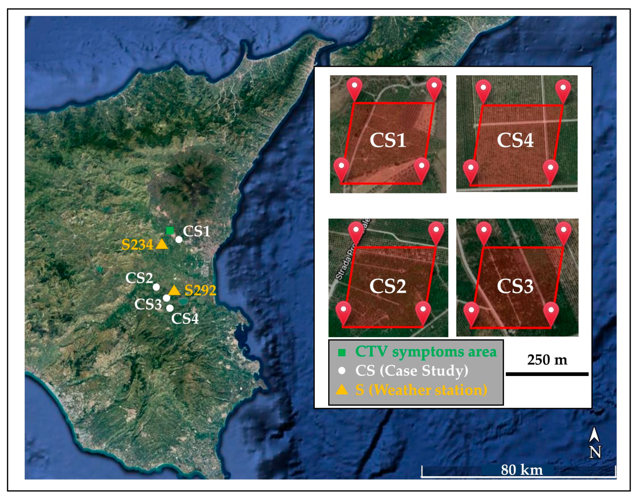
Figure 1. Map of the selected case studies (CSi I = 1, 4 at the Moderate Resolution Imaging Spectroradiometer (MODIS) pixel resolution) in Sicily with the indications of the first Citrus tristeza virus (CTV) focus area and of the meteorological stations.
Remotesensing 12 01965 g001
Figure 2. Sixteen-day averages of meteorological data (Tair, Rs, u2, P, RH) recorded at (a,b) S234 and (c,d) S292 weather stations during the available 2002–2018.
Remotesensing 12 01965 g002
Figure 3. Seasonality parameters generated in TIMESAT: (a) beginning of season, (b) end of season, (c) length of season, (d) base value, (e) time of middle of season, (f) maximum value, (g) amplitude, (h) small integrated value, (h + i) large integrated value. Graph provided by [41].
Remotesensing 12 01965 g003
Figure 4. Satellite images by Google Earth for CS1–CS4.
Remotesensing 12 01965 g004
Figure 5. Normalized Difference Vegetation Index (NDVI) temporal pattern observed at CS1–CS4 during the 2011–2018 period.
Remotesensing 12 01965 g005
Figure 6. Monthly NDVI box diagram observed at CS1–CS4 during 2001–2018.
Remotesensing 12 01965 g006
Figure 7. Original NDVI data from Terra-MODIS (in blue) and the fitted functions obtained by the double logistic filter curve fitting (CF) method in TIMESAT (in red) at (a) CS1, (b) CS2, (c) CS3 and (d) CS4.
Remotesensing 12 01965 g007
Figure 8. Seasonal parameters in CS1: (a) length value, (b) base value, (c) peak value, (d) amplitude value, (e) small seasonal integral and (f) large seasonal integral. Significant p-value (p < 0.05, 0.01 and 0.001) are indicated with *, ** and ***, respectively.
Remotesensing 12 01965 g008
Figure 9. Seasonal parameters in CS2: (a) length value, (b) base value, (c) peak value, (d) amplitude value, (e) small seasonal integral and (f) large seasonal integral. The grey areas refer to the time interval when corrective measures have been implemented for facing CTV. Significant p-value (p < 0.05, 0.01 and 0.001) are indicated with *, ** and ***, respectively.
Remotesensing 12 01965 g009
Figure 10. Seasonal parameters in CS3: (a) length value, (b) base value, (c) peak value, (d) amplitude value, (e) small seasonal integral and (f) large seasonal integral. The grey areas refer to the time interval when corrective measures have been implemented for facing CTV. Significant p-value (p < 0.05, 0.01 and 0.001) are indicated with *, ** and ***, respectively.
Remotesensing 12 01965 g010
Figure 11. Seasonal parameters in CS4: (a) length value, (b) base value, (c) peak value, (d) amplitude value, (e) small seasonal integral and (f) large seasonal integral. The grey areas refer to the time interval where corrective measures have been implemented for facing CTV. Significant p-value (p < 0.05, 0.01 and 0.001) are indicated with *, ** and ***, respectively.
Remotesensing 12 01965 g011
Figure 12. Matrix of the seasonal parameters in terms of R2.
Remotesensing 12 01965 g012
Table 1. Case studies’ (CS) main features.
ID PixelRootstockAge (years)Lat
(° N)
Long
(° E)
Elevation
(m, a.s.l.)
Area (ha)Planting Layout (m)
CS1Citrus aurantium L.4037.5214.921903.0 *4.5 × 4.5
CS26037.3714.82467.5 *4.5 × 4.5
CS33037.3714.89578.0 *4.5 × 4.5
CS42537.2714.886420.04.0 × 5.5
* the selected sites are homogeneous in terms of canopy ground cover within the MODIS pixel.
Table 2. Parameters setting in TIMESAT.
TIMESAT ParameterValue
CF methodDouble logistic
Seasonal parameter1
Spike method0
No. of envelop iterations1
Start of the season methodSeasonal amplitude
Season start, Season end0.2, 0.2
Table 3. Description of the seasonal parameters analyzed in the study.
Seasonal ParametersDescription
Length of the seasonTime from the “start” to the “end” of the season
Peak valueMaximum NDVI for the fitted function during the season
Base levelAverage of the left and the right minimum NDVI values
Seasonal amplitudeDifference between maximum NDVI and the base level
Small seasonal integralSmall integrated NDVI value for the fitted function during the season
Large seasonal integralIntegral of the function describing the season from the “start” to the “end”