Article

Stress Detection in New Zealand Kauri Canopies with WorldView-2 Satellite and LiDAR Data

1
Environmental Remote Sensing and Geoinformatics, Trier University, D-54296 Trier, Germany
2
Te Kura Ngahere School of Forestry, University of Christchurch, Christchurch 8041, New Zealand
3
Manaaki Whenua-Landcare Research, Palmerston North 4472, New Zealand
*
Author to whom correspondence should be addressed.
Remote Sens. 2020, 12(12), 1906; https://doi.org/10.3390/rs12121906
Submission received: 1 May 2020 / Revised: 5 June 2020 / Accepted: 8 June 2020 / Published: 12 June 2020
(This article belongs to the Special Issue Forest Canopy Disturbance Detection Using Satellite Remote Sensing)

Abstract

:
New Zealand kauri trees are threatened by the kauri dieback disease (Phytophthora agathidicida (PA)). In this study, we investigate the use of pan-sharpened WorldView-2 (WV2) satellite and Light Detection and Ranging (LiDAR) data for detecting stress symptoms in the canopy of kauri trees. A total of 1089 reference crowns were located in the Waitakere Ranges west of Auckland and assessed by fieldwork and the interpretation of aerial images. Canopy stress symptoms were graded based on five basic stress levels and further refined for the first symptom stages. The crown polygons were manually edited on a LiDAR crown height model. Crowns with a mean diameter smaller than 4 m caused most outliers with the 1.8 m pixel size of the WV2 multispectral bands, especially at the more advanced stress levels of dying and dead trees. The exclusion of crowns with a diameter smaller than 4 m increased the correlation in an object-based random forest regression from 0.85 to 0.89 with only WV2 attributes (root mean squared error (RMSE) of 0.48, mean absolute error (MAE) of 0.34). Additional LiDAR attributes increased the correlation to 0.92 (RMSE of 0.43, MAE of 0.31). A red/near-infrared (NIR) normalised difference vegetation index (NDVI) and a ratio of the red and green bands were the most important indices for an assessment of the full range of stress symptoms. For detection of the first stress symptoms, an NDVI on the red-edge and green bands increased the performance. This study is the first to analyse the use of spaceborne images for monitoring canopy stress symptoms in native New Zealand kauri forest. The method presented shows promising results for a cost-efficient stress monitoring of kauri crowns over large areas. It will be tested in a full processing chain with automatic kauri identification and crown segmentation.

Graphical Abstract

1. Introduction

The deadly kauri dieback disease (Phytophthora agathidicida (PA)) was first officially confirmed as a new pathogen by Beever in 2008 [1] in the Waitakere Ranges west of Auckland and later taxonomically described by Weir et al. [2]. Meanwhile, it was detected over most of the natural distribution range of New Zealand kauri [3]. The endemic kauri trees (Agathis australis) are a key species for the forest ecosystems on the North Island [4], a famous tourist attraction, and are of high cultural significance for Māori [5,6]. Regular monitoring of stress symptoms in tree canopies requires a cost-efficient, objective method that is suitable for covering large areas and able to detect the first signs of stress. Multispectral band and index combinations for the detection of kauri and canopy stress symptoms have been identified by Meiforth et al. [7,8]. Airborne Light Detection and Ranging (LiDAR) data recently became available for the northern kauri forests, so that the main part of the distribution range of kauri trees in New Zealand is now covered. In this study, we analyse the use of WorldView-2 (WV2) satellite data in combination with LiDAR data to detect stress symptoms in kauri trees in an object-based approach on manually segmented kauri crowns.

1.1. Kauri Trees and Kauri Dieback Symptoms

Kauri trees show a large phenological variety, from young conical trees with dense foliage to large open dome-shaped crowns (Figure 1). The mature trees develop a massive trunk and large side branches and reach heights of up to 40 m in the study areas. The colour of the foliage in non-symptomatic kauri varies from light green to a darker blue green, depending on the exposition to light and thickness of the wax coating. The flat lanceolate needle-like leaves create a spiky foliage surface. The foliage forms clusters in the medium growth stages and mature crowns show a more open canopy [5], with visible branch material and gaps from an aerial viewpoint. Stress symptoms of PA first become visible as yellowing and thinning of foliage, which exposes small top branches. Later stages of stress lead to structural changes caused by an ongoing loss of foliage, with an increase of visible bare branch material and gaps, until the tree dies [1,9]. The higher gap fraction increases the influence of undergrowth on the canopy reflectance. Small trees with a conical shape first develop a bare top on the main stem, while the foliage in the lower part of the canopy is affected in later stages. However, these types of symptoms can also have other causes, such as continuing drought periods [10], storm damage, or other diseases [1].

1.2. Research Background

High-resolution satellites have been successfully used to monitor forest health [13,14], both at a stand level [15,16,17,18,19] and individual tree crown level [20,21,22,23].
Amongst the most widely used vegetation indices for canopy stress detection with broader bandwidths of satellite images are combinations of near-infrared (NIR) and red bands, which are responsive to changes in canopy chlorophyll and leaf biomass. Other widely used indices are based on red and green bands sensitive to stress-related changes in leaf pigment compositions and bands in the NIR spectrum, which are influenced by the amount of leaf and canopy water and thus also structural changes due to foliage loss [13,24,25,26,27].
A new generation of commercial high-resolution satellites, such as WorldView (WV) and RapidEye (RE), launched in 2009 and 2008, respectively, has provided additional red-edge bands (WV, 705–745 nm; RE, 690–730 nm). In green vegetation, the red-edge region covers a steep increase in reflectance values between the red and NIR1 spectra and shows a high sensitivity to changes in chlorophyll, which causes a blue shift of the central red-edge region. Several studies have successfully applied spectral indices with red-edge bands from satellite data for stress detection in tree canopies. Oumar and Mutanga [28] utilised indices on the NIR and red-edge bands from WV2 data to detect a decline in Eucalypt plantations in South Africa. Ortiz et al. [17] detected early stages of bark beetle attack by combining TerraSAR-X and RapidEye data. Eitel et al. [29] proved that a normalised difference vegetation index (NDVI) with a red-edge band is suitable for detecting early stress symptoms in conifer woodland trees in New Mexico.
Textural information derived from satellite imagery has successfully been used to assess structural features in tree canopies [30,31,32]. It also has improved the analysis of stress symptoms in tree canopies, especially in later stages of decline with structural changes in the canopy [19,23].
Stress symptoms in kauri trees were analysed with airborne hyperspectral data by Meiforth et al. [8]. According to their study, a NIR/red NDVI, followed by indices with bands in the NIR and red-edge range are the most important for describing the full range of stress symptoms. However, pigment-sensitive indices with narrow green and red bands had a higher importance for the detection of stress symptoms in smaller crowns with denser foliage. Indices with NIR bands, such as the water band index (WBI) at 900 and 970 nm, were more relevant to describe stress symptoms in larger crown sizes with an open crown structure. The NIR bands are sensitive to structural changes and changes in the leaf water content. The paper recommends a stratified approach according to different growth stages of kauri.
An appropriate spatial resolution for the target objects is important for the successful use of satellite imagery in order to avoid mixed pixels with shadow, neighbouring vegetation, and soil [33]. In Meiforth et al. [8], a minimum crown diameter of 3 m was defined for stress detection in kauri trees for the 1 m resolution of a hyperspectral image. Fassnacht et al. [34] found that the 5 m pixel resolution of their HyMAP data (Integrated Spectronics) was too coarse to evaluate bark beetle infections at crown level. However, dead trees could still be mapped with a high overall accuracy (84–96%). Immitzer et al. [35] and Pu and Shawn [36] only used tree crowns that could be manually identified on WV2 respective Ikonos images. Immitzer et al. [35] defined at least two pixels (=4 m) per object as the minimum target size for an analysis of tree canopies with a WV2 image. Other studies analysed larger forest stands. Meddens et al. [37] discovered that a spatial resolution of 2.4 m performed best when mapping the infestation of forest stands with mountain pine beetle infection in Colorado. They demonstrated that a higher spatial resolution also increases the variability within the same level of crown damage and can cause a problematic “salt and pepper” effect in a pixel-based analysis. Lottering [38] and Ismail et al. [39] showed that higher-resolution data (1.25 and <1.75 m) are better suited to detecting early stages of stress in eucalyptus stands and a pine plantation, while later stages of stress are best described with lower spatial resolutions of 2.5 and 2.3 m. To achieve a sub-pixel horizontal accuracy in the processing of WV2 data, Aguilar et al. [40] recommended avoiding off-nadir angles higher than 20°. They achieved the highest spatial accuracies by using ortho-ready products with third order three-dimensional (3D) rational functions with the supplied rational polynomial coefficients, an accurate digital elevation model, and a polynomial adjustment with well distributed ground control points.
An object-based approach is well-suited to handling a high variance in target objects [41,42,43,44]. Several studies have found that object-based methods are superior to pixel-based methods for single tree crown analysis [35,45,46,47]. They have also been successfully applied for stress analysis and change detections in tree canopies [48,49,50]. For use in forest areas, an object-based approach requires a prior segmentation of crowns with respect to homogenous forest stands. An object-based analysis simplifies the combination of different data sources under the requirement that these are accurately aligned [51,52,53]. However, an essential condition for utilising the advantages of an object-based approach is that the pixel size is significantly smaller than the average size of the objects of interest [43].
The fusion of multispectral bands with a higher-resolution panchromatic channel, so-called pan-sharpening, allows the creation of a higher spatial resolution multispectral image. It can improve the use of textural attributes in an object-based analysis [54]. While some pan-sharpening methods can alter the spectral information, certain techniques, such as the Gram–Schmidt and Ehlers pan-sharpening methods, have been tested and shown to be superior for preserving the spectral values [55,56].
Stress symptoms in tree canopies caused by soil pathogens are expressed as a multifactor gradient with different states of chlorosis and defoliation until only bare branches are left [26]. While classification algorithms only distinguish between discrete classes, regression algorithms give a more detailed description of symptom stages with a continuous output. A regression approach also facilitates a more differentiated evaluation of changes in a time series. Training based on the correlation coefficient allows regression models to handle a high variance in the data. Several studies have successfully used regression approaches to analyse stress symptoms in tree canopies [19,57], predict tree mortality [58], and evaluate foliar moisture [59]. However, a non-linear relationship in the numeric range of reference values causes a shift between the scales of the reference and predicted values. Meiforth et al. [8] enhanced the linearity by rescaling the value range and also suggested testing a two-step approach, in which the dead and dying trees are first identified in a binary classification. The remaining stress levels can then be analysed in a regression approach.
Light Detection and Ranging (LiDAR) systems generate an accurate, high-resolution, three-dimensional point cloud, which enables to segment single tree crowns and homogenous units of forest stands [60,61,62,63,64,65]. LiDAR data allows estimating crown parameters, such as the tree height, crown shape, canopy density, foliage texture, and structural crown characteristics [66,67]. The LiDAR intensity values add a spectral component as the amount of reflected energy at the peak amplitude of the returned LiDAR signal in the near-infrared region, usually at 1064 or 1550 nm. Intensity data have been successfully used to describe tree canopies and detect tree species [61,68,69,70]. The suitability of LiDAR attributes for assessing structural crown characteristics as a measure of defoliation has been proven in Scots pine forests at both stand level [71,72,73] and single tree level [72]. In combination with biochemical and biophysical information from passive optical sensors, LiDAR data can demonstrably enhance individual tree analysis [35,52,61,74,75]. The combination of different data sources requires accurate spatial alignment. Data from airborne LiDAR systems (ALS) are usually the remote sensing data with the highest spatial accuracy compared, for example, to photogrammetric data [76,77]. However, the accuracy of terrain models derived from ALS ground data is impaired in terrain with steep slopes and vegetation with dense foliage and undergrowth [76,78].

1.3. Objectives

Spectral indicators with a sensitivity to stress symptoms in kauri trees have already been defined by Meiforth et al. [8] for use with an airborne multispectral system. This study analyses whether these findings can be implemented in an operational detection strategy based on WV2 satellite data. With LiDAR data available for most of the distribution range of New Zealand kauri, LiDAR-based crown attributes were integrated for crown stratification and to test their use for stress detection. The study pays special attention to differentiating early signs of stress. It has the following objectives:
  • Test the performance of WV2 attributes for crown-based stress detection in kauri trees and define the recommended minimum crown size;
  • Test a two-step method on WV2 attributes by first identifying dead and dying trees in a classification and then applying a regression for the remaining stress symptom levels;
  • Test the performance of LiDAR attributes in combination with WV2 data for canopy stress detection.
A minimum requirement for the performance of the developed method for a value range of symptom levels from 1 to 5 is a root mean square error (RMSE) smaller than 0.5, so that the predicted symptom values stay mainly within one reference symptom level. While the analysis in this study is based on manually edited crowns, the application for monitoring requires additional steps to automatically pre-segment crowns with respect to homogenous stand units for the existing LiDAR data and to define kauri trees. To prepare for this full workflow, we edited the reference crowns for this study on the LiDAR data.

2. Materials and Methods

2.1. Study Area

The Waitakere Ranges on the west coast of Auckland are amongst the highest PA-affected forest areas, and the first officially confirmed site in New Zealand with a verified PA infection (Figure 2a, [1]). The Ranges are characterised by a warm temperate climate and a rough terrain, with steep slopes and elevations from sea level to 474 m [79]. The three selected study sites (Figure 2b) cover trees with the full range of symptom stages in both homogenous and mixed stands, with mainly second-growth kauri forests in the Maungaroa area, larger trees in the Kauri Grove area, and all growth stages of kauri in the Cascades.

2.2. LiDAR Data and Aerial Images

Airborne LiDAR data were obtained for the study areas on 30 January 2016 by AAM New Zealand, with a Q1560 LiDAR sensor (400 kHz, 58° field of view) [11]. The sensor achieved five pulses/m2 on average, which resulted in 35 average returns/m2 and 0.17 m average point spacing. The ground return, however, was significantly less, with 0.8–1.5 ground returns per m2 in the dense forest stands. The sensor utilises the 1064 nm wavelength to record intensity. The spatial accuracy was stated as +/−0.1 m standard error for vertical information and +/− <0.5 m standard error for horizontal information at a 68% confidence level.
A digital terrain model (DTM), digital surface model (DSM), and ground normalised crown height model (CHM) were generated in LAStools [83] with the “spike-free” method, according to Khosravipoura et al. [84]. Outliers that were classified as “noise” were removed. The method uses all returns to create a triangular irregular network (TIN) from the highest returns downwards. The user defines a “freeze distance” for the maximum length of the triangle sides, and an “insertion buffer” in a vertical downward direction, which defines the points that are included in the TIN creation, before the freezing process starts. All triangles with sides shorter than the freeze distance are preserved and underlying points are ignored in further steps of the TIN creation for the remaining LiDAR points. This method prevents the creation of downward spikes. In the final step, the surface model is created through a linear interpolation of the spike-free TIN. As a rule of thumb, the lengths of the triangle sides should be around three times the average pulse spacing. We calculated two versions of height models with freeze distances of 0.6 m and 1 m and a pixel size of 0.25 m, which is larger than the average pulse spacing of the last returns of 0.23 m for this dataset.
A three-band red-green-blue (RGB) aerial image was acquired during the same flight as the LiDAR data collection, with a 15 cm pixel resolution. It was delivered in two versions: orthorectified on the surface model and the terrain model [11]. Another aerial image was obtained by order of the Auckland Council in May 2017, with three RGB bands at a 7.5 cm resolution and orthorectified on a DTM [12].

2.3. WorldView-2 Image

The WV2 image was captured on 15 March 2017 at 11:33 a.m. (local time) during cloud-free conditions with 45.7° sun elevation and 18.2° off-nadir angle. It covers 100 km2 of the Waitakere Ranges (Figure 2b) and was delivered as standard imagery with nearest neighbour resampling in an “ortho ready” format. The eight multispectral bands have a resolution of 1.8 m, and the pan channel features a 0.45 m resolution (Table 1, Figure 3). They reach up to 1043 nm in wavelength, but do not reach the characteristic spectral pattern of kauri trees in the NIR2 range (Figure 3).
Atmospheric correction of the multispectral bands was carried out with the Fast Line-of-sight Atmospheric Analysis of Hypercubes (FLAASH) module in ENVI, which incorporates the MODerate resolution atmospheric TRANsmission (MODTRAN) radiation transfer model [85]. The eight multispectral bands were pan-sharpened to a 0.5 m resolution with the Gram–Schmidt method [86] using ENVI’s Spectral Processing Exploitation and Analysis Resource (SPEAR) tools. The Gram–Schmidt method performs well in retaining spectral information [55,87] and has been used in several studies with satellite images for the analysis of tree canopies [88,89]. The image was orthorectified using ENVI’s orthorectification tool for WV2 images with the rational polynomial coefficients (RPCs) provided by Digital Globe with the image (Figure A1, Appendix A). The orthorectification included a 1 m DEM (spatial accuracy at 95% confidence: vertical +/−0.2 m, horizontal +/−0.6 m) for the entire area [90]. Remaining deviations were addressed with a shift in the X and Y direction and a georeferencing with a second-order polynomial transformation based on 1102 ground control points (GCPs) for the three areas. The mean control point error for the WV2 image in the three study areas was an RMSE of 0.87 m (X 0.57 m, Y 0.66 m). Shadow areas were defined with a threshold value of 300 on a brightness layer, to match manually identified outer crown shadows while keeping internal crown shadows. The brightness layer was calculated as the average of the blue, green, red, and NIR1 bands [91].

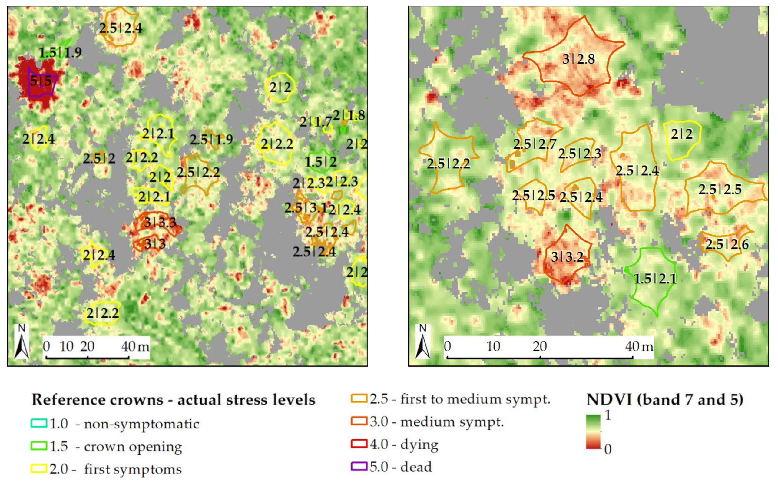
2.4. Reference Crown Set

The reference crown set with 1089 crowns of kauri and dead/dying trees is based on the crown locations and attributes acquired during fieldwork in the summer of 2015/16 and complemented and updated during the summer season of 2016/2017 [7,8] (Table 2). The recorded crown attributes in the field include basic metrics, such as the stem diameter at breast height, the cardinal crown spread, and the canopy base height, as well as a detailed description of canopy characteristics, such as an estimated crown density, coverage in percentage classes [93], and the amount of dead branches [93]. In addition, other signs of stress were recorded such as decolouration of the foliage and the number of epiphytes. The crowns used in this analysis have a mean diameter of at least 3 m and were stratified into three growth stages using the mean crown diameter (Figure 1). An outer buffer of 10% of the mean crown diameter was removed before the analysis to reduce edge effects and effects of a spatial misalignment between the LiDAR CHM and the WV2 image. After removing the shadow areas, only crowns with sunlit areas larger than 50% compared to the full crown size were considered for the analysis.

2.5. Reference Values for Stress Assessment

An overall canopy score for stress symptoms was assessed for each crown at five levels, from 1 for non-symptomatic dense foliage, to 5 for “dead tree”. This score was based on the fieldwork and the assessment of aerial images, according to the method described by Meiforth et al. [8]. For a more detailed evaluation of the first stress symptoms, the stress levels 1 to 2 were refined in half-steps (Figure 4) for this study. Level 1 describes crowns with non-symptomatic dense green foliage, which is mainly found in small and some medium crowns. Level 1.5 applies to crowns with still green, but more open foliage, with exposed gaps and single patches of visible branch material from an aerial viewpoint. This level is typically found in non-symptomatic medium and larger crowns. The stress level 2 features visible smaller branches over the full crown extent and the partial yellowing of foliage. Further increasing gaps and visible small to medium bare branches are the main visible characteristics of level 2.5 in the aerial images, as well as a more intense yellowing in some trees. Level 3 features large branches that become visible as linear structures. Level 4 marks a degree of foliage loss that deteriorates the overall crown architecture and shows a decolouration from yellow-green to brown in the remaining foliage. Level 5 describes dead crowns and also includes different amounts of photosynthetic active undergrowth and epiphytes. Figure 5 gives an impression of the crown polygons for different forest stands on the WV2 image with an indication of the crown stress symptom values.
To account for the fact that the LiDAR data were acquired in 2016, one season before the WV2 image, the aerial images from both years were compared, and crowns that showed visible changes or where the status of the crown could not be identified on both aerial images were removed. Since both summers were relatively moist, the stress symptoms had not changed as rapidly as in a drought situation.

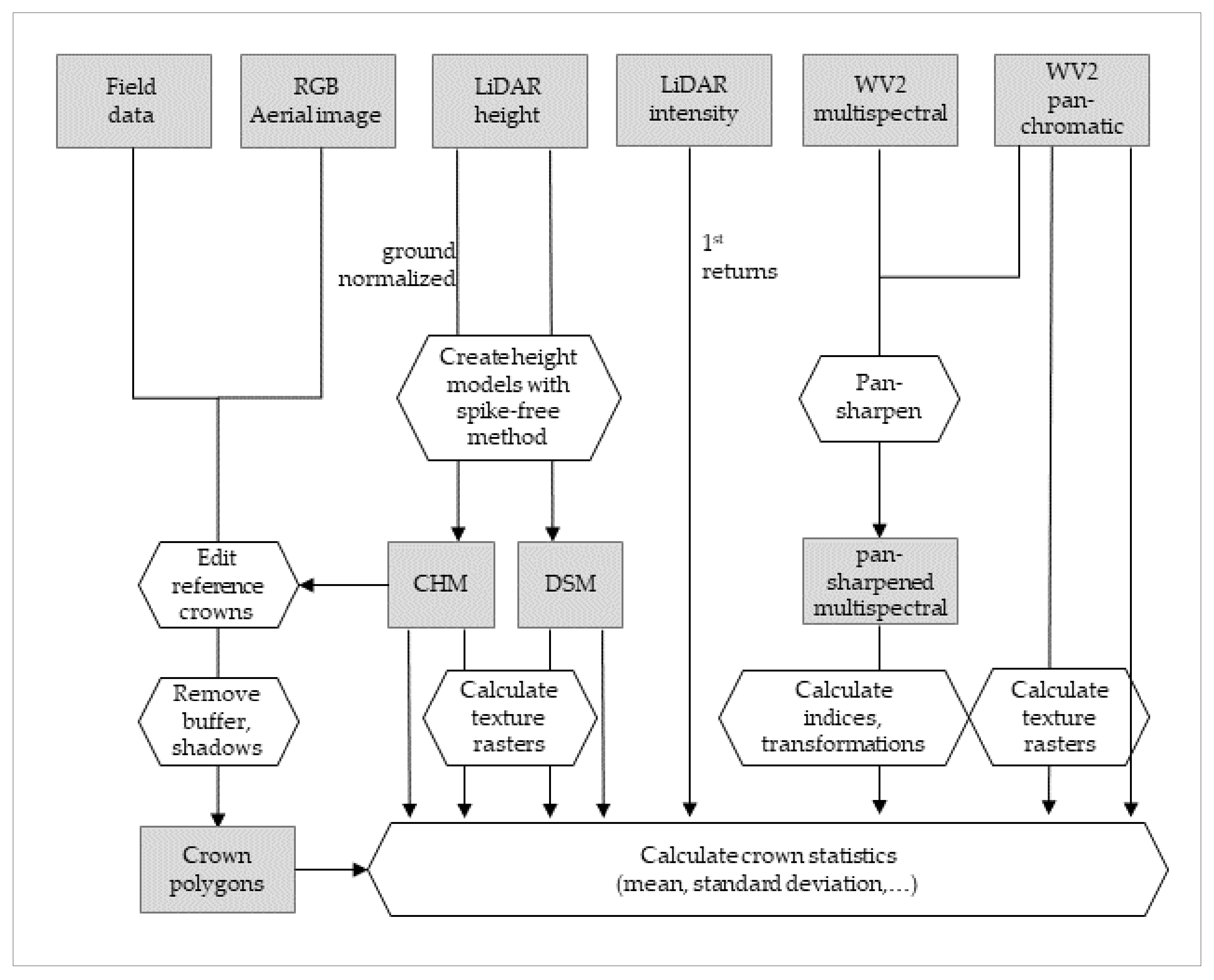
2.6. Attribute Calculation

A total of 203 LiDAR attributes was calculated for crown stratification and stress detection. For the stratification of crown sizes, basic crown metrics were derived from the coarser CHM with the 1 m spike-free threshold, such as the maximum crown height and mean diameter. Figure 6 gives an overview of the workflow for the attribute calculation.
For stress detection, LiDAR attributes were calculated on both versions of the DSM and CHM (0.6 m and 1 m spike-free threshold). They describe the shape, crown structure, and texture. The range of attributes covers height ratios, percentiles and bincentiles, point density and coverage, shape, roundness, slope, and curvatures, as well as first- and second-order texture measures, such as variance, range, kurtosis, homogeneity, and skewness (see Table A1, Appendix C). These measures were either calculated directly on the LiDAR point cloud for the crown polygons or first calculated as rasters with different kernel sizes. We also calculated statistics from the intensity values of the first returns. Height cut-offs of 6 and 8 m for calculation of the density and coverage on the LiDAR point cloud for low and high stands were derived from the field measurements of the canopy base height. Table A1 in Appendix C gives an overview of the attributes and tools.
Spectral (43) and textural (111) attributes were calculated on the eight pan-sharpened multispectral WV2 bands with the band math tool in ENVI. The original set of 31 calculated vegetation indices is based on literature research. They also include the best performing indices from the hyperspectral analysis presented in Meiforth et al. [8], as far as the wavelengths and bandwidths of the WV2 image allowed for a calculation. In addition to the indices, bands from a minimum noise fracture (MNF) transformation, a three-band Munsell hue, saturation, and value transformation (HSVM), and a brightness layer [91] were calculated. In total, 110 texture rasters were based on the PAN channel and band 7 with occurrence and co-occurrence matrices on different kernel sizes. For more details, see Table A2 in Appendix C.
The rasters were scaled to the 1–99 or 2–98 percentiles, according to the histogram distribution, to remove outliers. The resulting attribute rasters were aggregated on the crown polygons with the zonal statistic tool in QGIS by the mean crown value and the standard deviation for the spatial attributes.

2.7. Attribute Selection and Regression Approach

The aim of the attribute selection was to identify the subset of attributes with the highest correlation to the stress symptom levels. First, highly correlated and redundant attributes were removed. The attributes were clustered according to their origin (WV2, LiDAR height, and LiDAR intensity) and function as spectral or structural. In each of the clusters, pre-selection was performed with a Wrapper Subset Evaluator [94,95], which outperformed other subset selection methods, such as the correlation-based feature selection (Cfs) and classifier subset evaluator. We used the open source data mining software WEKA, which was developed by Waikato University in New Zealand [96].
The wrapper method evaluates attribute combinations with a specified machine learning algorithm based on a defined evaluation criterion. We used a random forest (RF) regression in 200 iterations, with the Pearson correlation coefficient (correlation) as the evaluation measure. The RF regression also corresponds to the algorithm used for the analysis in this paper and a former analysis of kauri stress symptoms [8]. RF is a non-parametric algorithm that does not require a certain distribution of data [97]. It can handle a large number of input variables with a high variance and is less sensitive to overfitting, unless the data is noisy [98]. To avoid overfitting, we tested and pruned the RF tree to a maximal depth of eight. We tested several search methods and “best first” with bidirectional selection, and a search termination of eight consecutive non-improving nodes gave the best results. The “best first” method combines a backward elimination with a forward selection by finding the best attribute subset from the Wrapper Subset Evaluator. The pre-selected subsets were complemented with other attributes highly correlated to the stress levels, which were identified with the correlation attribute evaluator in WEKA. The subset selection of all attributes was repeated with different seed values. Depending on the number of attributes selected, the resulting attributes from all subsets were again combined, and the subset selection was repeated with a different range of seed values, in order to reduce the selection to the most relevant attributes. Figure 7 shows four raster images of the selected attributes.
The performance of each subset from the final selection round was then tested in an RF regression with a three-fold split and 1000 repetitions, to define the best performing subset. The correlation, the root mean squared error (RMSE), and the mean absolute error (MAE) were calculated as evaluation metrics. When two subsets performed equally well, the one with fewer attributes was chosen. The importance of each attribute in the final selection was calculated as the average impurity decrease for the RF regression.
We also tested an approach that was discussed in Meiforth et al. [8], by first identifying the dead and dying trees in a binary RF classification, before applying a regression for the lower symptom levels.

3. Results

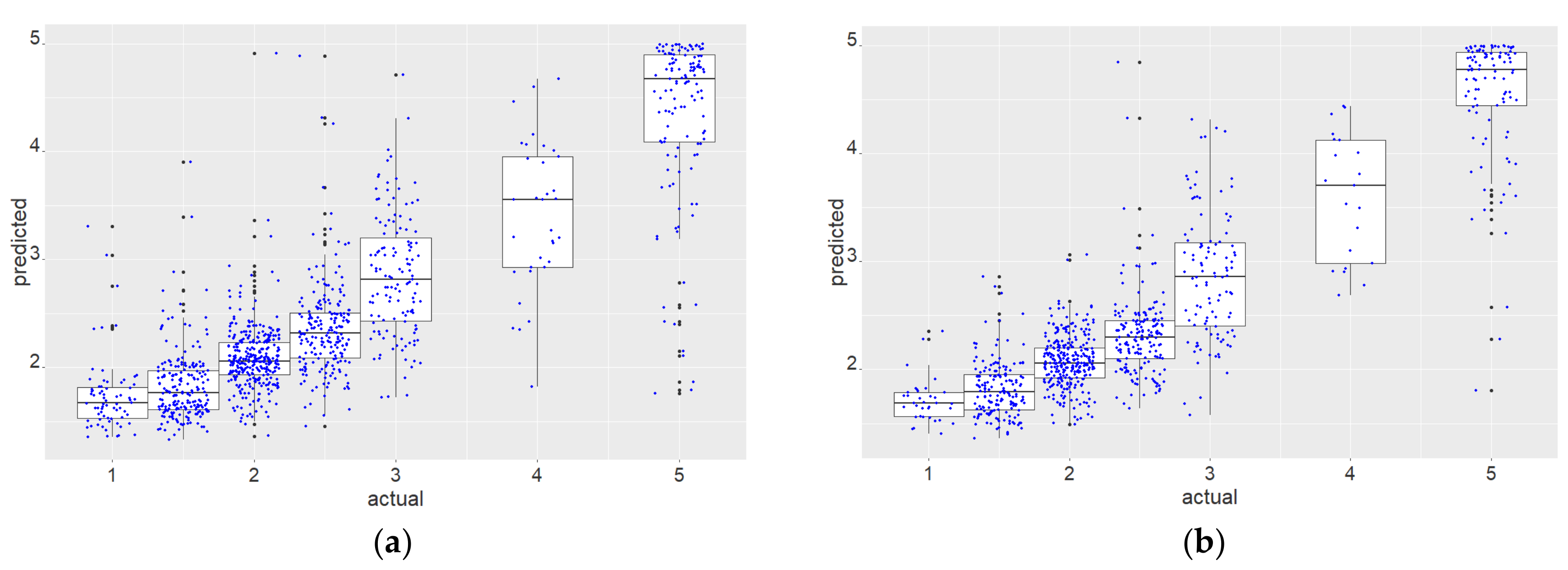
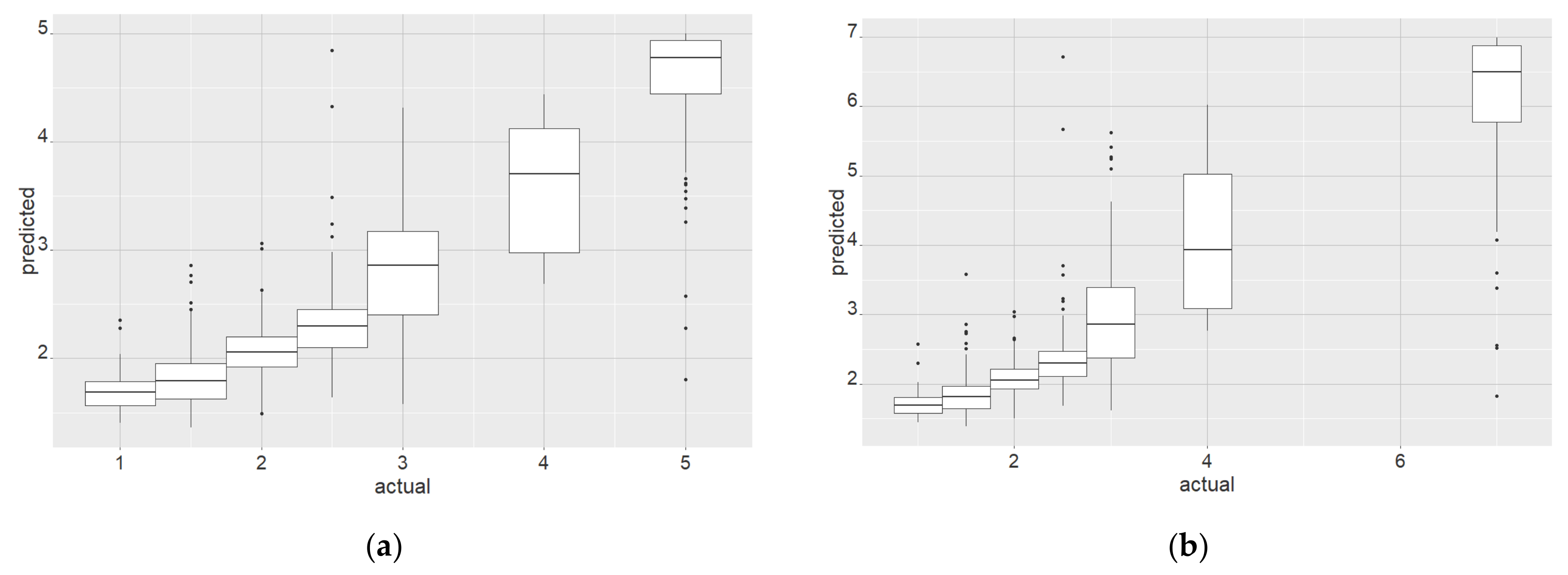
3.1. Results Objective 1: Test the Performance of WV2 Attributes for Crown-Based Stress Detection in Kauri Trees and Define the Recommended Minimum Crown Size

A selection of eight WV2 attributes and the maximum crown height resulted in a correlation of 0.85 and an RMSE of 0.59 for all 1089 crowns with a minimum diameter of 3 m (Table 3, Table A3 in Appendix D). For a minimum crown diameter of 4 m, the correlation increased to 0.89, while the RMSE decreased to 0.48 (Table 3). Figure 8 and Figure 9 show that mainly the small crown sizes and higher stress levels caused outliers (error >1).
To analyse the effect of spatial misalignment between the WV2 image and the CHM, we measured the spatial deviation between both datasets for 100 randomly selected crown polygons (Figure A2, Appendix B). The test resulted in an overall RMSE of 0.87 m, with 60 crowns having no position error. After subtracting a buffer of 10% of the mean crown diameter, 90% of the remaining crown polygons (edited on the CHM) were within 0.5 m of the crown position on the WV2 image. However, the horizontal inaccuracy of six of the 100 crowns on the WV2 image accounted for more than 20% of their mean crown diameter (mean crown size 6.3 m, standard deviation 3.0 m).
The boxplot diagram in Figure 10a confirms the overall good match of the model, with a correlation of 0.89 for all crowns with a diameter larger than 4 m. However, the first quartiles of the half-step levels (1 to 1.5 and 2 to 2.5) and the levels 3 and 4 overlap, while the first quartiles of the other levels are more separated. The diagram also shows a slightly non-linear relationship between the actual and predicted values, especially towards the dead and dying trees. After a rescaling of the value for dead trees from 5 to 7, a more linear relationship could be established, facilitating the interpretation of the results (Figure 10b). The correlation for the rescaled value range remained unchanged, while the RMSE and MAE values increased with the higher value range.
The most important attributes are a combination of red/NIR1 bands in a normalised vegetation index (NDVI_75), followed by a ratio of the red and green bands (red-green ratio index (RGRI)) and the standard deviation of the first band of an MNF transformation (Table 4). For mean crown values of a green NDVI (NDVIg) with red-edge and green bands, the red-edge band and a brightness layer were also selected. Further attributes include the mean value of a seven-pixel kernel of the PAN band and the range of a three-pixel kernel on the NIR1 band. Figure 11 illustrates the predicted versus the actual stress values and their match with an NDVI_75 raster.
An M5P and linear regression resulted in slightly lower correlations (0.87 and 0.86, respectively) and higher RMSE values (0.52 and 0.55, respectively) compared to the RF regression (correlation of 0.89, RMSE of 0.48) for the seven stress levels and crowns with a diameter larger than 4 m.
A comparison with a reference scheme on the basic five stress levels showed a lower performance (correlation of 0.88, RMSE of 0.55) than the seven-level reference scheme with a more detailed assessment of the first symptoms (Table 5 and Table A3 in Appendix D). While the NDVIg and red-edge band were not selected for the five stress levels, a ratio of the two NIR bands (modified normalised difference water index (mNDWI)) improved the performance.

3.2. Results Objective 2: Classification to Identify Dead and Dying Trees

Dying and dead trees (level 4 and 5) with a diameter larger than 4 m could be identified in an RF classification based on WV2 attributes, with a user’s accuracy of 84.3% and a producer’s accuracy of 88.7% (Table 6). The remaining stress levels from 1 (non-symptomatic) to 3 (medium symptoms) could be described for crowns larger than 4 m, with an RMSE value of 0.37 (MAE of 0.28, correlation of 0.72). The main differences in the attribute selection to the full symptom range are the higher importance of the NDVIg with red-edge and green bands and the selection of the mNDWI on the NIR bands for the first stress levels from 1 to 3 (Table A3 in Appendix D).

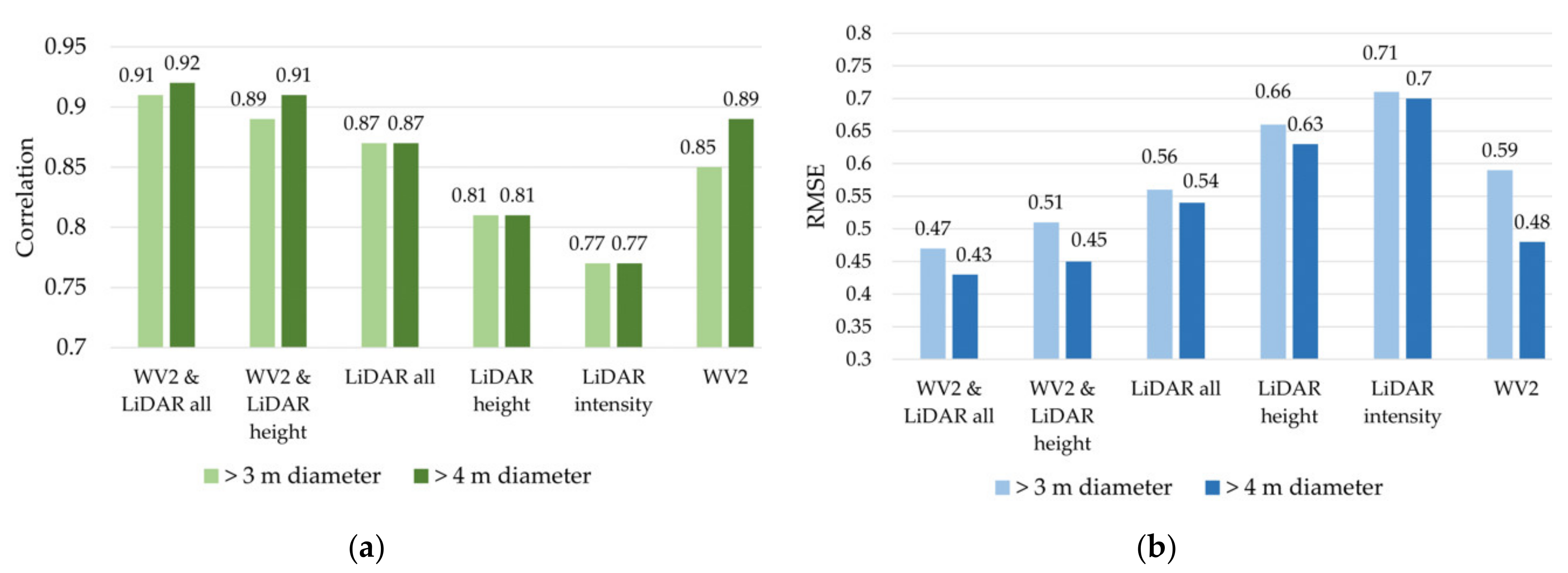
3.3. Results Objective 3: Test the Performance of LiDAR Attributes for Stress Detection

The combination with LiDAR attributes improved the stress detection compared to only WV2 attributes for all tested reference schemes (Table 7). For crowns larger than 4 m and seven stress levels, the correlation increased from 0.89 to 0.92 and the RMSE was lowered from 0.49 to 0.43. While the removal of very small crowns under 4 m diameter notably improved the correlation and RMSE for WV2 attributes, the correlation for only LiDAR attributes did not change and the RMSE only improved slightly (Figure 12).
The most important attributes for a combination of LiDAR and WV2 data (Table 8) are the NDVI on the red/NIR1 bands, followed by the ratio between the maximum height and the 50th percentile crown height (R_max_P50) and the average intensity values. The standard deviation of the first MNF band was also selected with a high importance amongst other spatial attributes for crowns with a diameter larger than 4 m.
Both the identification of dead and dying trees (Table 9, Table A4 in Appendix E), as well as the detection of first stress symptoms (level 1 to 3), improved with additional LiDAR attributes. In the attribute selection for the first stress symptom, the intensity values had a higher importance, while the R_max_P50 and brightness attributes were not selected (Table 8).

4. Discussion

The high overall performance of WV2 attributes with a correlation of 0.89 (RMSE of 0.48, MAE of 0.34) for the seven stress symptom levels and crowns with a diameter larger than 4 m diameter showed that WV2 data is well-suited to describe stress symptoms in kauri canopies. The seven-level reference scheme includes a refined description of the first stress symptoms, which is important for an early identification of potentially infected stands.

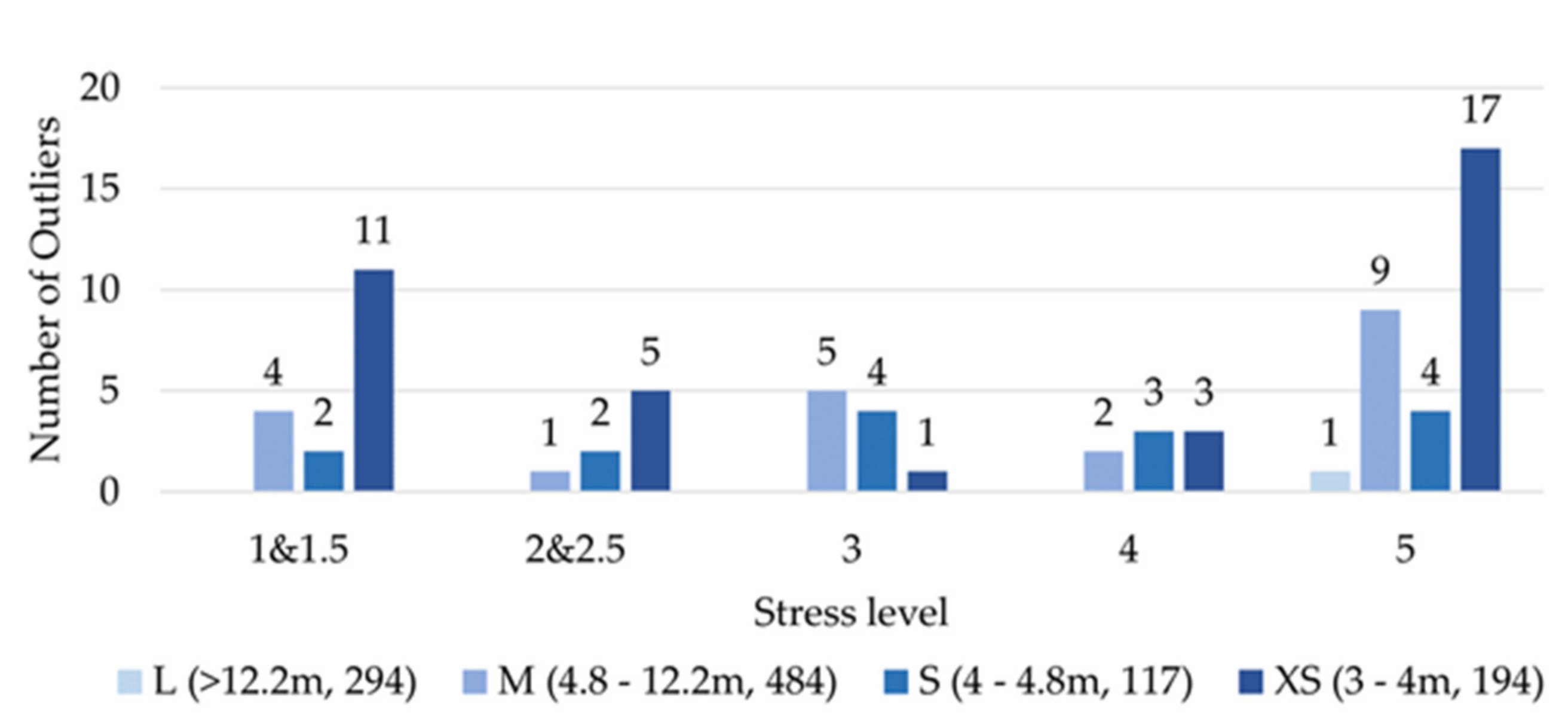
4.1. Discussion: Minimum Crown Size, Spatial Accuracy and Stratified Approach

The high number of outliers in crowns with a diameter smaller than 4 m, especially for dead and dying trees, is an indicator that the multispectral resolution of 1.8 m in the WV2 image causes mixed pixels in small crowns and is too coarse to detect the small bare top branch of severely affected small crowns. For the use of only WV2 attributes on the full range of stress symptoms, a minimum crown size of at least 4 m is recommended, which improves the correlation from 0.85 to 0.89 and the RMSE from 0.59 to 0.48. Stands with kauri of smaller crown sizes should be pre-segmented and analysed in homogenous stand units.
Spatial misalignment between the WV2 image and the CHM also caused errors. This cannot be completely avoided, especially in steep terrain with high crown heights [106]. The subtraction of an outer buffer of 10% of the mean crown diameter helped to reduce the effects of spatial inaccuracy. However, still six of the 100 tested crown polygons showed displacements of more than 20% of the remaining mean crown diameter. To improve the spatial accuracy, the use of a DSM instead of a DEM should be tested for orthorectification. The different appearance of kauri growth stages requires a stratified approach [8]. If only WV2 data are available for regular monitoring, the inclusion of the maximum crown height derived from LiDAR data of former years allows such a stratification.

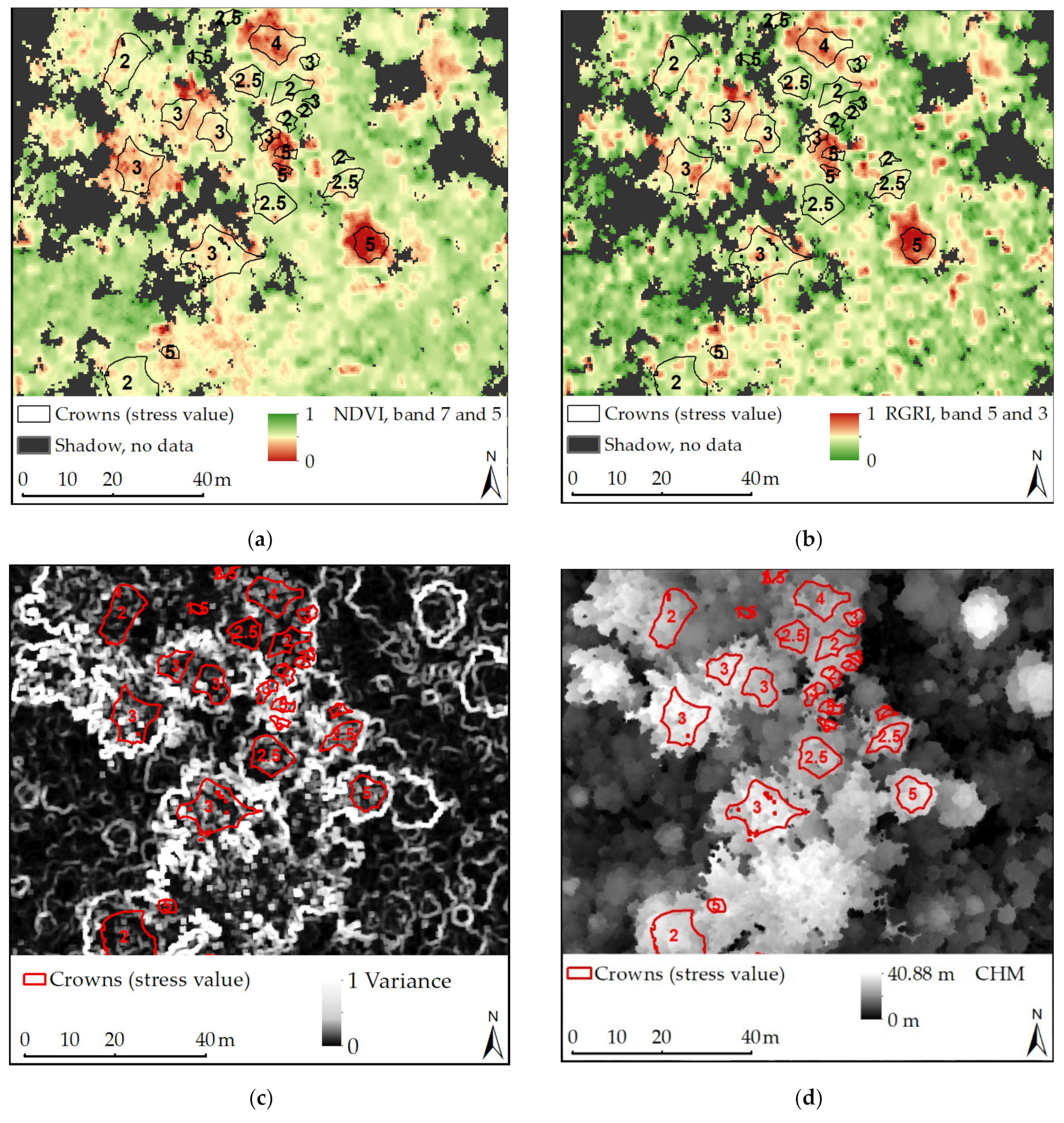
4.2. Discussion: Attribute Performance

According to the findings presented in Meiforth et al. [8], an NDVI with a red and NIR1 band combination (NDVI_75) and a red-green ratio (RGRI) are the most important attributes for stress detection in the full seven-level symptom range (32.5% and 25% importance, respectively), including dead and dying trees. While the NDVI_75 saturates for high chlorophyll and biomass levels, it is able to capture the loss of photosynthetic activity and structural changes caused by foliage loss [99,100]. The also selected RGRI combination, the green NDVI (9.2% importance), and the mean of the red-edge band (3.7%) are more sensitive to pigment changes [103,107]. The standard deviation of the first band of an MNF transformation (12.6% importance) and the range of the NIR1 band (4.3%) provide information on structural and textural crown characteristics, which are influenced by a higher number of large bare branches and internal shadows. The same features are also captured by a selected brightness layer (3.9%). These attributes have a higher importance in a five-level reference scheme with a greater emphasis on advanced stress levels (Table A3, Appendix D).
For the detection of the first stress symptoms in trees with a still intact crown architecture (level 1 to 3), the green NDVI has higher importance. It detects the blue shift of the red-edge point caused by a decline in photosynthetic activity and changes in the foliage pigment concentrations [107]. A modified normalised difference water index (mNDWI) for the NIR1 and NIR2 bands was also selected for the first stress levels, and is sensitive to a reduction of leaf-cell wall scattering and reduced canopy water caused by foliage loss [108].

4.3. Discussion: Dealing with Non-Linearity: Rescaling and a Two-Step Approach

While the RF regression is well suited to handle non-linear relationships, the boxplot in Figure 10a shows that the medians of the resulting values for dead and dying crowns are slightly lower than the actual values. This effect of non-linearity is mainly caused by the more extreme reflectance values of dead branches and shadows in the later stages of decline.
A rescaling of the reference values for the dead crowns (i.e., subdividing the range for this crown state in several levels of severity) suggested by Meiforth et al. 2020 [8] leads to a better match between the medians of the results compared to the actual values (Figure 10b), while the overall correlation coefficients remain unchanged. Merging the mapped severity classes again after the prediction process allows to maintain the original value range from 1 (non-symptomatic) to 5 (dead), which also corresponds to the field reference scheme used by the Auckland Council. A change detection however should be based on the original resulting values to utilise the detailed information in the continuous output range of the regression analysis.
The test of a two-step approach showed that the identification of dead and dying crowns in a binary RF classification requires additional LiDAR data for a stress description of crown sizes smaller than 4 m. If only WV2 attributes are available, the minimum crown size should be 4 m mean diameter. Although, even for crowns larger than 4 m, ca. 15% of the dead and dying crowns were still misclassified as less symptomatic. The remaining lower stress levels from 1 to 3 can be described in a regression with the pre-selected attribute sets with an RMSE of 0.37. However, the mistakes from prior classification need to be added to these results, which makes the interpretation more complicated, especially when this method is used in a change detection. For an easier interpretation, we recommend using only a regression approach.

4.4. Discussion: Performance of Additional LiDAR Attributes for Stress Detection

The improved performance with additional LiDAR attributes for stress detection can be explained by the additional 3D information in higher spatial resolution, the high spatial accuracy and the spectral information in the intensity values. Moreover, there is no misalignment with the crown polygons, since the reference crowns were manually edited on the LiDAR data.
The ratio between the maximum crown height and 50th percentile height has high importance for reference schemes that include dead and dying crowns, but it was not selected to assess the first stress symptoms. The advanced loss of foliage is characterised by a lower 50th percentile height of the LiDAR returns, while the maximum height in the form of branches still remains high, even in the later stress stages, caused by the remaining (dead) branches. Further selected LiDAR height attributes describe textural characteristics, as an indicator of foliage loss that exposes gaps and bare branches, such as the variance, standard deviation, and cross curvature in CHM and DSM models. The performance of these attributes depends on an accurate spatial alignment, since their values increase on the edge of the crowns (Figure 7c). For the time being, the acquisition of airborne LiDAR data is still too expensive for regular monitoring of stress symptoms. However, the inclusion of the maximum crown height enables a size stratification and improves the performance of the stress detection with the WV2 data. For the stratification, the crown height can also be derived from older LiDAR data.

4.5. Discussion: Recommendations for Further Studies

The resulting stress symptom values of the remote sensing analysis need to be interpreted to translate them into health categories by local experts considering the growth stage, the stand situation, the environmental conditions, and other possible causes of stress. Spatiotemporal dynamics of stress symptoms over several years analysed in change detections might also help to distinguish between PA infection and other causes of stress [16,109,110]. We also recommend testing the use of the original, not pan-sharpened multispectral bands, especially for stress detection in medium and larger crown sizes.
Further studies should investigate crown and stand segmentation in kauri forests based on LiDAR data. Zörner et al. [111] developed a method for large tree detection in native New Zealand forest in the Wellington region. Another promising method for canopy segmentation was developed by Wagner et al. [65] in an Atlantic rainforest based on a U-net convolutional network.
A stand-based analysis of stress symptoms with satellite data requires a better understanding of spectral stress responses in associated tree species. Meiforth et al. [7] showed that the effect of waxy, shiny foliage surface in kahikatea, wooden seed capsules in kānuka, and the influence of older needle cohorts in perennial conifers like rimu can lead to confusion with dead and dying crowns [7]. A spectral unmixing of forest stands with known spectra of kauri and other tree species might also help with the interpretation of stress assessment in mixed forest stands [33,112,113].
We also recommend testing the use of other datasets, which offer more cost-efficient options, such as optical height models derived from Stereo-VHR, instead of LiDAR [114]. Additionally, the newly launched constellations of micro-satellites could be tested, which offer opportunities for producing very-high spatial resolution data at a relatively low cost [115].

5. Conclusions

This study presents a method for detecting stress symptoms in the canopies of New Zealand kauri trees with LiDAR and WV2 data. A unique characteristic of this study is the large representative reference dataset with 1089 manually edited crowns. It covers the full range of stress symptoms and size classes of kauri in different stand situations. A reference scheme for stress symptoms in five levels was refined to seven levels with a higher differentiation of the first stages of stress. A crown diameter of 4 m was determined as the recommended minimum object size for stress detection, to avoid higher numbers of outliers and mixed pixels for smaller crown sizes. The removal of a 10% outer crown buffer helped to reduce edge effects and spatial misalignment. A selection of eight WV2 attributes in combination with the maximum crown height resulted in a correlation of 0.89 (RMSE of 0.48, MAE of 0.34) in an RF regression for crown sizes larger than 4 m. The performance could be further improved by adding LiDAR attributes (correlation of 0.92, RMSE of 0.43). For cost-efficient regular monitoring of stress symptoms, we recommend the use of WV2 satellite data on pre-segmented crowns with a diameter larger than 4 m and homogenous stand units for smaller crown sizes. The maximum crown height should be included in the analysis to allow for stratification. With the newly available LiDAR data for crown segmentation over the main distribution area of natural kauri forests, the results of this study have important implications for cost-efficient large area monitoring of stress symptoms in New Zealand’s kauri forests.

Author Contributions

Conceptualisation, J.J.M., J.H., J.D.S. and J.R.D.; methodology, J.J.M., J.H. and H.B.; software, J.J.M.; validation, J.J.M.; formal analysis, J.J.M.; investigation, J.J.M.; resources, J.J.M. and J.D.S.; data curation, J.J.M.; writing—original draft preparation, J.J.M.; writing—review and editing, J.J.M., H.B., J.H., J.D.S. and J.D.; visualisation, J.J.M.; supervision, H.B., J.H. and J.D.S.; project administration, J.J.M. and J.H.; funding acquisition, J.J.M., J.H., J.D.S. and J.R.D. All authors have read and agreed to the published version of the manuscript.

Funding

The Kauri Dieback Programme (NZ) funded most of the remote sensing data (Ministry for Primary Industries agreement nr 17766), while the University of Canterbury (NZ), Landcare Research (NZ) (through MBIE contract C09X1709), the University of Trier (Germany), and FrontierSI (former CRCSI) Australia supported living costs, fieldwork, equipment, and additional LiDAR data. Auckland Council supported the fieldwork and supplied LiDAR data and aerial images. The DigitalGlobe Foundation granted satellite images. Rapidlasso and Harris Geospatial supplied grants for software licenses. Henning Buddenbaum was supported within the framework of the EnMAP project (FKZ 50 EE 1530) by the German Aerospace Center (DLR) and the Federal Ministry of Economic Affairs and Energy. Landcare Research funded the publication costs.

Acknowledgments

Our sincere thanks go to all people and institutions who supported this project. We are especially grateful to David Norton, who helped with the administration and provided input for the fieldwork and ecological aspects of the analysis. Nick Waipara, Lee Hill, and Yue Chin Chew from Auckland Council helped to establish the project and provided data. The Kauri Dieback Programme (Planning and Intelligence Team) gave constructive feedback and support during this research. We would also like to thank the staff of the Arataki visitor centre, Fredrik Hjelm from the Living Tree Company, and Joanne Peace for their excellent support and guidance during the fieldwork. Our thanks go to Massey University for the provision of the hyperspectral data acquisition, as well as AAM NZ Ltd. for the acquisition and processing of airborne LiDAR data. Jeanette Allen, Vicki Wilton, and Nicole Gellner helped with the university administration.

Conflicts of Interest

The authors declare no conflict of interest.

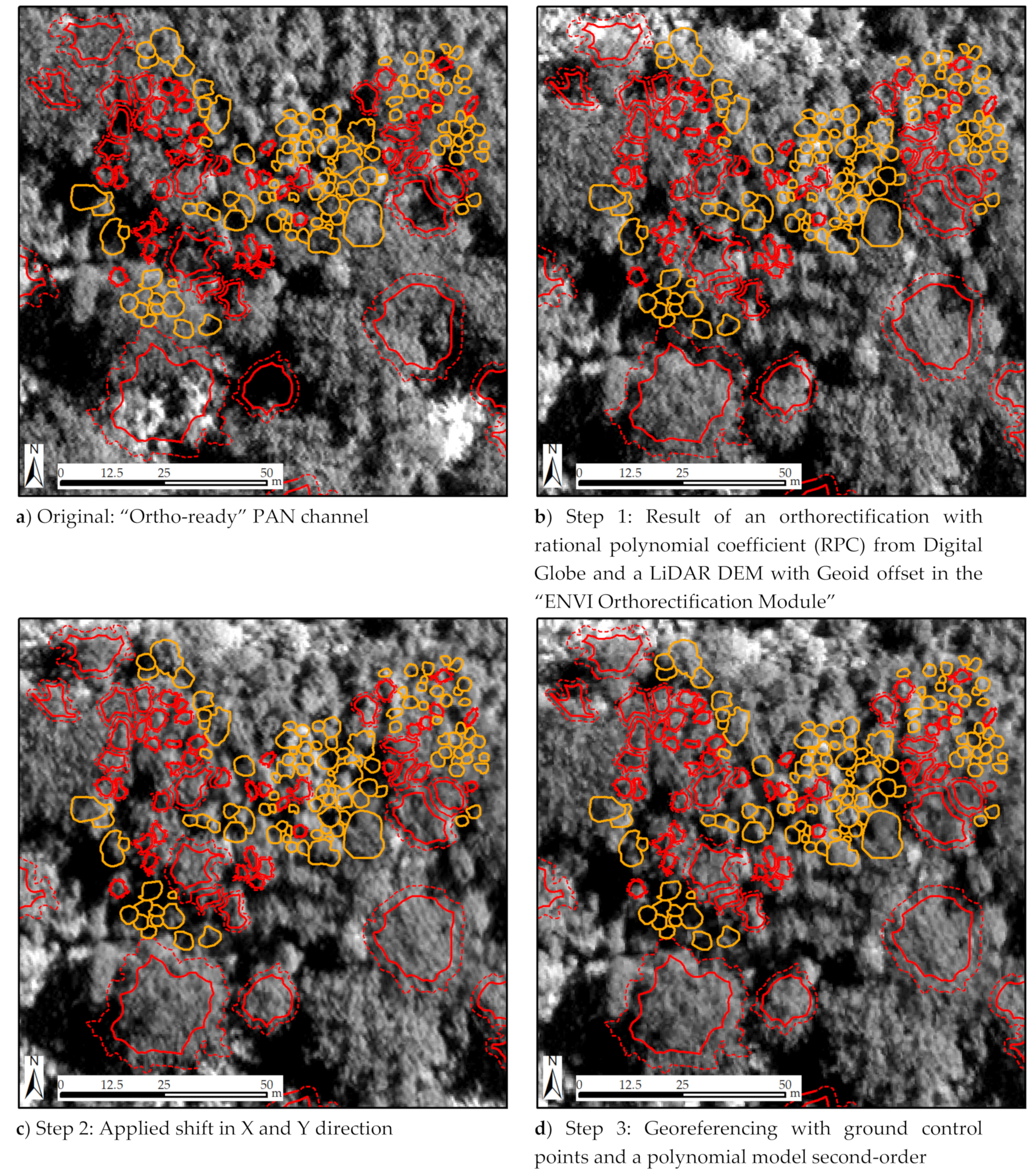
Appendix A. Illustrations for the Orthorectification of the WV2 Image

Figure A1. Different steps in the orthorectification illustrated with the PAN channel of the WorldView-2 image, for a forest section in the Cascade area. The red polygons mark crowns of kauri and dead/dying trees that were used in the analysis. The 10% buffer, which was removed for the analysis, is marked with a stippled line. The orange polygons mark crowns from other species and kauri smaller than 3 m diameter that were not used in this study.
Remotesensing 12 01906 g0a1

Appendix B. Spatial offset of crown polygons to WV2 Image

Figure A2. Spatial offset of crown polygons, edited on the LiDAR CHM, to the WorldView-2 image, measured for 100 randomly selected crowns. The offset is marked in classes with (a) the distance in percent from the crown diameter and (b) the absolute distance in meter. The blue values mark the offset for the full crown polygons, and the green values mark the offset for the inner buffer that was used in the analysis, after a 10% outer buffer was removed.
Remotesensing 12 01906 g0a2

Appendix C. LiDAR and WorldView-2 Attributes

Table A1. LiDAR attributes (203 total).
TotalBased onAttributesSoftware/Tools
14Intensity valuesAvg, qav, std, ske, kur
Percentiles (01, 05, 10, 25, 50, 75, 90, 95, 99)
LAStools, LAScanopy
88DSM 1Stdev, var, rang, crosc, longc, mnc, mxc, slp, avgdev, kur, skw, on 3 × 3, 5 × 5, 7 × 7 kernel sizeQGIS zonal statistic,
GRASS: r.param.scale
55CHM 1Mean, max, st. dev., rang, med, maj, var, vart, prc conv, sa, var, ent, asm, con, cor,
idm, con, cor> all attributes were calculated on 3, 5, 7 kernel sizes
QGIS zonal statistic
GRASS: r.statistics, r.texture, r.slope.aspect
13Crown polygonRatio mdm/height;
Ratio of max height with 95th, 75th, and 50th percentiles and average height of outer crown edge;
difference of max height with 75 and 50 percentile, peak density, height, mdm, shp area and roundness (shp area/lengths), average height of outer crown edge
ArcGIS tools
33LiDAR point cloudStd, ske, kur, cov, dns (cut value 6 m and 8 m), min, max, avg, avg 1st return, percentiles (01, 05, 10, 25, 50, 75, 90, 95, 99), bincentiles (10, 20, 30, 40, 50, 60, 70, 80, 90)LAStools
LAScanopy
1 The digital surface model (DSM) and the crown height model (CHM) were calculated with LAStools as spike-free rasters, according to Khosravipoura et al. [84], in two versions with a “freeze distance” of 60 and 100 cm.
Table A2. Attributes calculated on the WorldView-2 image (154 total).
TotalAttributes 2Crown StatisticsSoftware/Tools
8multispectral bands 1–8meanENVI
1MNF transformation (1st band)st. dev.ENVI
4HSVM transformation (3 bands), brightness layer (1 band)meanENVI
3131 vegetation indicesmeanENVI
110textures on PAN channel and band 7 (NIR1) with 3 × 3, 5 × 5, and 7 × 7 kernels: rang, mean, var, ent, skw, hom, con, cor, sm, dis 2mean
st. dev.
ENVI
2 Abbreviations for Table A1 and Table A2.
asmangular second m
avg average
avgdev average deviation
con contrast
cor correlation
cov coverage
crosc cross-sectional curvature
dis dissimilarity
dns density
ent entropy
hom homogeneity
idm inverse difference
kur kurtosis
longc longitudinal curvature
maj majority
mdm mean diameter
med median
mnc mean curvature
mxc max curvature
planc plan curvature
prc convpercent convex
profc profile curvature
qav quadratic average
rang range
skw skewness
slp slope
sm second moment
st. dev. standard deviation
var variance
vart variety

Appendix D. WV2 Attribute Importance for the Basic and Refined Symptom Levels

Table A3. Selected attributes and attribute importance in percent for different stress symptom references (basic 5 levels 1, first symptoms 2, refined 7 levels 3) based on crowns with a diameter larger than 4 m for WV2 attributes. The attribute importance for an RF regression was calculated as the average impurity decrease and converted to percentages.
Abbrev.Band5 LevelFirst7 LevelCrown StatisticDescriptionAlgorithmRef.
Imp. %Imp. %Imp. %
NDVI5, 732.226.731.5meanNDVI(b7 − b5)/(b7 + b5) 4[99,100]
RGRI3, 529.520.324.2meanRed-Green Ratio Indexb5/b3 4[101]
MNF1all15.29.912.3st. dev.1st band of an MNF transformation [102]
NDVIg3, 6 13.19meanGreen NDVI(b6 − b3)/(b6 + b3)) 4[103]
mNDWI7, 85.05.7 meanmodified Normalized Difference Water Index(b7 − b8)/(b7 + b8) 4[108]
Bright2, 3, 5, 74.7 3.8meanbrightness band(b2 + b3 + b5 + b7)/4 4[91]
b66 3.6meanmean of band 6
b7_3krg7 7.44.2meanrange of a 3 × 3 kernel on band 7 [104]
b7_5krg7 8.8 st. dev.range of a 5 × 5 kernel on band 7 [104]
Pn_k7smPAN3.7 meansecond moment of a 3 × 3 kernel on the PAN band [104]
Pn_k7mnPAN3.68.02.7st. dev.mean of a 7 × 7 kernel on the PAN band [104]
CHM 6.2 5.7maxmaximum height on CHM raster
(spike-free threshold 1 m)
[84]
1 Five-level value range (1–2–3–4–5); 2 First symptoms value range (1–1.5–2–2.5–3); 3 Seven level value range (1–1.5–2–2.5–3–4–5); 4 The variables marked with “b” indicate the band numbers of the WV2 image, according to Table 1.

Appendix E. WV2 and LiDAR Attributes to Identify Dead and Dying Trees

Table A4. Selected attributes to identify dead and dying trees for all crown sizes (total 1089) with a random forest classifier based on WV2 attributes only (WV2) and in combination with LiDAR attributes (WV2 and LiDAR). The attribute importance (imp.)was calculated as the average impurity decrease.
Abbrev.CrownDescriptionWV2WV2 and LiDARRef.
Statistic 1089 Crowns
>3 m
895 Crowns
>4 m
1089 Crowns
>3 m
895 Crowns
>4 m
imp. %corr.imp. %corr.imp. %corr.imp. %corr.
NDVI_75meanNDVI (b7 − b5)/(b7 + b5) 1 25.80.75 15.70.75[99,100]
MCARI1meanModified Chlorophyll Absorption in Reflectance Index 11.2*(2.5*[b7-b5]-1.3*[b7-b3]) 1 16.20.39[116]
NDVIgmeangreen NDVI (b6 − b3)/(b6 + b3)) 126.70.55 [103]
RDVImeanRenormalized Difference Vegetation Index (b7−b5) /sqrt(b7+b5) 122.20.51 [116,117]
ARVImeanatmospherically resistant vegetation index
(b7) - (2*b5-b2)/(b7) + (2*b5-b2) 1
18.50.70 16.50.70 [118]
MNF_1stst. dev.1st band of an MNF transformation 15.50.65[102]
Pan_k3skmeanskewness of a 3 × 3 kernel on the PAN band17.20.01 [104]
Brightmeanbrightness band (b2 + b3 + b5 + b7)/4 1 20.20.06 [91]
Pan_k3hmmeanhomogeneity of a 3 × 3 kernel on the PAN band 21.40.10 [104]
Pan_k5Crmeancorrelation of a 5 × 5 kernel on the PAN band 15.70.03 [104]
b7_k3rgmeanrange of a 3 × 3 kernel on the band 715.50.0216.90.0718.20.0216.40.07[104]
intensityskewnessLiDAR intensity value 14.70.5512.10.52[83]
D6_k5varvariancevariance of a 5 × 5 kernel on the DSM (spike-free threshold 0.6 m) 13.80.17 [104]
Cg6_k5varmedianvariance of a 5 × 5 kernel on the CHM (spike-free threshold 0.6 m) 12.30.51[104]
RatDMHght ratio between the mean diameter and maximum height 13.60.00
R_max_P50 ratio between the maximum height and the 50th percentile 11.40.58
CHMmaximummaximum height on CHM raster (spike-free threshold 1 m) 11.80.2811.80.27[84]
1 The variables marked with “b” indicate the band numbers of the WV2 image according to Table 1.

References

  1. Beever, R.E.; Waipara, N.W.; Ramsfield, T.D.; Dick, M.A.; Horner, I.J. Kauri (Agathis australis) under threat from Phytophthora. Phytophthoras For. Nat. Ecosyst. 2009, 74, 74–85. [Google Scholar]
  2. Weir, B.S.; Paderes, E.; Anand, N.; Uchida, J.Y.; Pennycook, S.R.; Bellgard, S.E.; Beever, R.E. A taxonomic revision of Phytophthora Clade 5 including two new species, Phytophthora agathidicida and P. cocois. Phytotaxa 2015, 205, 21–38. [Google Scholar] [CrossRef]
  3. MPI. Map “Kauri Dieback Distribution”. Available online: https://www.kauridieback.co.nz/media/2037/kauri-dieback-distribution_20190930_350dpi.jpg (accessed on 20 February 2020).
  4. Ecroyd, C.E. Biological flora of New Zealand 8.Agathis australis (D. Don) Lindl. (Araucariaceae) Kauri. New Zealand J. Bot. 1982, 20, 17–36. [Google Scholar] [CrossRef]
  5. Steward, G.A.; Beveridge, A.E. A review of New Zealand kauri (Agathis australis (D. Don) Lindl.): Its ecology, history, growth and potential for management for timber. N. Z. J. For. Sci. 2010, 40, 33–59. [Google Scholar]
  6. Shortland, T.; Wood, W. Kia Toitu He Kauri, Kauri Dieback Tangata Whenua Roopu Cultural Impact Assessment. Report by Repo Consultancy Ltd., Comissioned by the Ministry of Primary Industries NZ/the Kauri Dieback Programme. Available online: https://www.kauridieback.co.nz/media/1813/shortland-wood-2011.pdf (accessed on 5 March 2020).
  7. Meiforth, J.J.; Buddenbaum, H.; Hill, J.; Shepherd, J.; Norton, D.A. Detection of New Zealand Kauri Trees with AISA Aerial Hyperspectral Data for Use in Multispectral Monitoring. Remote Sens. 2019, 11, 2865. [Google Scholar] [CrossRef] [Green Version]
  8. Meiforth, J.; Buddenbaum, H.; Hill, J.; Shepherd, J. Monitoring of Canopy Stress Symptoms in New Zealand Kauri Trees Analysed with AISA Hyperspectral Data. Remote Sens. 2020, 12, 926. [Google Scholar] [CrossRef] [Green Version]
  9. Bellgard, S.; Weir, B.; Pennycook, S.R.; Paderes, E.P.; Winks, C.; Beever, R.E.; Williams, S. Specialist Phytophthora Research: Biology, Pathology, Ecology and Detection of PTA; Final Report for the New Zealand Ministry for Primary Industries: Wellington, New Zealand, 2013. [Google Scholar]
  10. Macinnis-Ng, C.; Schwendenmann, L. Litterfall, carbon and nitrogen cycling in a southern hemisphere conifer forest dominated by kauri (Agathis australis) during drought. Plant. Ecol. 2015, 216, 247–262. [Google Scholar] [CrossRef]
  11. Ministry of Primary Industries. Airbone LiDAR and RGB Aerial Images in the Waitakere Ranges; Ministry of Primary Industries: Wellington, New Zealand, 2016.
  12. Auckland Council 0.075m Urban Aerial Photos RGB, Waitakere Ranges. Available online: https://data.linz.govt.nz/layer/95497-auckland-0075m-urban-aerial-photos-2017/ (accessed on 12 April 2019).
  13. Wang, J.; Sammis, T.; Gutschick, V.P.; Gebremichael, M.; Dennis, S.O.; Harrison, R.E. Review of Satellite Remote Sensing Use in Forest Health Studies. Open Geogr. J. 2010, 3, 28–42. [Google Scholar] [CrossRef]
  14. Pause, M.; Schweitzer, C.; Rosenthal, M.; Keuck, V.; Bumberger, J.; Dietrich, P.; Heurich, M.; Jung, A.; Lausch, A. In Situ/Remote Sensing Integration to Assess Forest Health—A Review. Remote Sens. 2016, 8, 471. [Google Scholar] [CrossRef] [Green Version]
  15. Townsend, P.A.; Singh, A.; Foster, J.; Rehberg, N.J.; Kingdon, C.C.; Eshleman, K.; Seagle, S.W. A general Landsat model to predict canopy defoliation in broadleaf deciduous forests. Remote Sens. Environ. 2012, 119, 255–265. [Google Scholar] [CrossRef]
  16. Garrity, S.R.; Allen, C.D.; Brumby, S.P.; Gangodagamage, C.; McDowell, N.G.; Cai, D.M. Quantifying tree mortality in a mixed species woodland using multitemporal high spatial resolution satellite imagery. Remote Sens. Environ. 2013, 129, 54–65. [Google Scholar] [CrossRef]
  17. Ortiz, S.M.; Breidenbach, J.; Kändler, G. Early Detection of Bark Beetle Green Attack Using TerraSAR-X and RapidEye Data. Remote Sens. 2013, 5, 1912–1931. [Google Scholar] [CrossRef] [Green Version]
  18. Dotzler, S.; Hill, J.; Buddenbaum, H.; Stoffels, J. The Potential of EnMAP and Sentinel-2 Data for Detecting Drought Stress Phenomena in Deciduous Forest Communities. Remote Sens. 2015, 7, 14227–14258. [Google Scholar] [CrossRef] [Green Version]
  19. Meng, J.-H.; Li, S.; Wang, W.; Liu, Q.; Xie, S.; Ma, W. Mapping Forest Health Using Spectral and Textural Information Extracted from SPOT-5 Satellite Images. Remote Sens. 2016, 8, 719. [Google Scholar] [CrossRef] [Green Version]
  20. White, J.C.; Wulder, M.A.; Brooks, D.; Reich, R.; Wheate, R.D. Detection of red attack stage mountain pine beetle infestation with high spatial resolution satellite imagery. Remote Sens. Environ. 2005, 96, 340–351. [Google Scholar] [CrossRef]
  21. Nitesh, P.; Ismail, R. Discriminating the occurrence of pitch canker fungus inPinus radiatatrees using QuickBird imagery and artificial neural networks. South. For. A J. For. Sci. 2013, 75, 29–40. [Google Scholar] [CrossRef]
  22. Waser, L.T.; Küchler, M.; Jütte, K.; Stampfer, T. Evaluating the Potential of WorldView-2 Data to Classify Tree Species and Different Levels of Ash Mortality. Remote Sens. 2014, 6, 4515–4545. [Google Scholar] [CrossRef] [Green Version]
  23. Wang, H.; Pu, R.; Zhang, Z.; Zhao, Y. Mapping Robinia Pseudoacacia Forest Health Conditions by Using Combined Spectral, Spatial and Textureal Information Extracted from Ikonos Imagery. ISPRS—Int. Arch. Photogramm. Remote Sens. Spat. Inf. Sci. 2016, 1425–1429. [Google Scholar] [CrossRef] [Green Version]
  24. Tuominen, J.; Lipping, T.; Kuosmanen, V.; Haapane, R. Remote Sensing of Forest Health. In Geoscience and Remote Sensing; IntechOpen: London, UK, 2009. [Google Scholar]
  25. Jones, H.G.; Vaughan, R.A. Remote Sensing of Vegetation: Principles, Techniques, and Applications; Oxford University Press: Oxford, UK, 2010. [Google Scholar]
  26. Lausch, A.; Erasmi, S.; King, D.; Magdon, P.; Heurich, M. Understanding Forest Health with Remote Sensing -Part I—A Review of Spectral Traits, Processes and Remote-Sensing Characteristics. Remote Sens. 2016, 8, 1029. [Google Scholar] [CrossRef] [Green Version]
  27. Thenkabail, P.S.; Lyon, J.G.; Huete, A. Fundamentals, Sensor Systems, Spectral Libraries, and Data Mining for Vegetation; CRC Press: Boca Raton, FL, USA, 2018. [Google Scholar]
  28. Oumar, Z.; Mutanga, O. Integrating environmental variables and WorldView-2 image data to improve the prediction and mapping of Thaumastocoris peregrinus (bronze bug) damage in plantation forests. ISPRS J. Photogramm. Remote Sens. 2014, 87, 39–46. [Google Scholar] [CrossRef]
  29. Eitel, J.U.H.; Vierling, L.A.; Litvak, M.E.; Long, D.S.; Schulthess, U.; Ager, A.A.; Krofcheck, D.J.; Stoscheck, L. Broadband, red-edge information from satellites improves early stress detection in a New Mexico conifer woodland. Remote Sens. Environ. 2011, 115, 3640–3646. [Google Scholar] [CrossRef]
  30. Kayitakire, F.; Hamel, C.; Defourny, P. Retrieving forest structure variables based on image texture analysis and IKONOS-2 imagery. Remote Sens. Environ. 2006, 102, 390–401. [Google Scholar] [CrossRef]
  31. Ozdemir, I.; Karnieli, A. Predicting forest structural parameters using the image texture derived from WorldView-2 multispectral imagery in a dryland forest, Israel. Int. J. Appl. Earth Obs. Geoinformation 2011, 13, 701–710. [Google Scholar] [CrossRef]
  32. Eckert, S. Improved Forest Biomass and Carbon Estimations Using Texture Measures from WorldView-2 Satellite Data. Remote Sens. 2012, 4, 810–829. [Google Scholar] [CrossRef] [Green Version]
  33. Somers, B.; Verbesselt, J.; Ampe, E.; Sims, N.; Verstraeten, W.; Coppin, P. Spectral mixture analysis to monitor defoliation in mixed-aged Eucalyptus globulus Labill plantations in southern Australia using Landsat 5-TM and EO-1 Hyperion data. Int. J. Appl. Earth Obs. Geoinf. 2010, 12, 270–277. [Google Scholar] [CrossRef]
  34. Fassnacht, F.E.; Latifi, H.; Ghosh, A.; Joshi, P.K.; Koch, B. Assessing the potential of hyperspectral imagery to map bark beetle-induced tree mortality. Remote Sens. Environ. 2014, 140, 533–548. [Google Scholar] [CrossRef]
  35. Immitzer, M.; Atzberger, C.; Koukal, T. Tree Species Classification with Random Forest Using Very High Spatial Resolution 8-Band WorldView-2 Satellite Data. Remote Sens. 2012, 4, 2661–2693. [Google Scholar] [CrossRef] [Green Version]
  36. Pu, R.; Landry, S. A comparative analysis of high spatial resolution IKONOS and WorldView-2 imagery for mapping urban tree species. Remote Sens. Environ. 2012, 124, 516–533. [Google Scholar] [CrossRef]
  37. Meddens, A.J.H.; Hicke, J.A.; Vierling, L.A. Evaluating the potential of multispectral imagery to map multiple stages of tree mortality. Remote Sens. Environ. 2011, 115, 1632–1642. [Google Scholar] [CrossRef]
  38. Lottering, R.; Mutanga, O. Optimising the spatial resolution of WorldView-2 pan-sharpened imagery for predicting levels of Gonipterus scutellatus defoliation in KwaZulu-Natal, South Africa. ISPRS J. Photogramm. Remote Sens. 2016, 112, 13–22. [Google Scholar] [CrossRef]
  39. Ismail, R.; Mutanga, O.; Kumar, L.; Bob, U. Determining the optimal spatial resolution of remotely sensed data for the detection of sirex noctilio infestations in pine plantations in KwaZulu-Natal, South Africa. S. Afr. Geogr. J. 2008, 90, 22–31. [Google Scholar] [CrossRef]
  40. Aguilar, M.A.; del Mar Saldana, M.; Aguilar, F.J. Assessing geometric accuracy of the orthorectification process from GeoEye-1 and WorldView-2 panchromatic images. Int. J. Appl. Earth Obs. Geoinf. 2013, 21, 427–435. [Google Scholar] [CrossRef]
  41. Van de Voorde, T.; De Genst, W.; Canters, F.; Stephenne, N.; Wolff, E.; Binard, M. Extraction of land use/land cover related information from very high resolution data in urban and suburban areas. Remote Sensing in Transition. In Proceedings of the 23rd Symposium of the European Association of Remote Sensing Laboratories, Ghent, Belgium, 2–5 June 2003; pp. 237–244. [Google Scholar]
  42. Gao, Y.; Mas, J.F. A comparison of the performance of pixel-based and object-based classifications over images with various spatial resolutions. Online J. Earth Sci. 2008, 2, 27–35. [Google Scholar]
  43. Blaschke, T. Object based image analysis for remote sensing. ISPRS J. Photogramm. Remote Sens. 2010, 65, 2–16. [Google Scholar] [CrossRef] [Green Version]
  44. Boggs, G. Assessment of SPOT 5 and QuickBird remotely sensed imagery for mapping tree cover in savannas. Int. J. Appl. Earth Obs. Geoinformation 2010, 12, 217–224. [Google Scholar] [CrossRef]
  45. Yan, G.; Mas, J.F.; Maathuis, B.H.F.; Xiangmin, Z.; Van Dijk, P. Comparison of pixel-based and object-oriented image classification approaches—A case study in a coal fire area, Wuda, Inner Mongolia, China. Int. J. Remote Sens. 2006, 27, 4039–4055. [Google Scholar] [CrossRef]
  46. Weih, R.C.; Riggan, N.D. Object-based classification vs. pixel-based classification: Comparative importance of multi-resolution imagery. Int. Arch. Photogramm. Remote Sens. Spat. Inf. Sci. 2010, 38, C7. [Google Scholar]
  47. Whiteside, T.G.; Boggs, G.; Maier, S. Comparing object-based and pixel-based classifications for mapping savannas. Int. J. Appl. Earth Obs. Geoinf. 2011, 13, 884–893. [Google Scholar] [CrossRef]
  48. Desclée, B.; Bogaert, P.; Defourny, P. Forest change detection by statistical object-based method. Remote Sens. Environ. 2006, 102, 1–11. [Google Scholar] [CrossRef]
  49. Stagakis, S.; Gonzalez-Dugo, V.; Cid, P.; Guillén-Climent, M.; Zarco-Tejada, P.J. Monitoring water stress and fruit quality in an orange orchard under regulated deficit irrigation using narrow-band structural and physiological remote sensing indices. ISPRS J. Photogramm. Remote Sens. 2012, 71, 47–61. [Google Scholar] [CrossRef] [Green Version]
  50. Gärtner, P.; Förster, M.; Kurban, A.; Kleinschmit, B. Object based change detection of Central Asian Tugai vegetation with very high spatial resolution satellite imagery. Int. J. Appl. Earth Obs. Geoinf. 2014, 31, 110–121. [Google Scholar] [CrossRef]
  51. Sasaki, T.; Imanishi, J.; Ioki, K.; Morimoto, Y.; Kitada, K. Object-based classification of land cover and tree species by integrating airborne LiDAR and high spatial resolution imagery data. Landsc. Ecol. Eng. 2011, 8, 157–171. [Google Scholar] [CrossRef]
  52. Zhang, Z.; Liu, X. WorldView-2 satellite imagery and airborne LiDAR data for object-based forest species classification in a cool temperate rainforest environment. In Developments in Multidimensional Spatial Data Models; Springer: Berlin, Germany, 2013; pp. 103–122. [Google Scholar]
  53. Machala, M. Forest Mapping Through Object-based Image Analysis of Multispectral and LiDAR Aerial Data. Eur. J. Remote Sens. 2014, 47, 117–131. [Google Scholar] [CrossRef]
  54. Wang, H.; Pu, R.; Zhu, Q.; Ren, L.; Zhang, Z. Mapping health levels of Robinia pseudoacacia forests in the Yellow River delta, China, using IKONOS and Landsat 8 OLI imagery. Int. J. Remote Sens. 2015, 36, 1114–1135. [Google Scholar] [CrossRef]
  55. Nikolakopoulos, K. Quality assessment of ten fusion techniques applied on Worldview-2. Eur. J. Remote Sens. 2015, 48, 141–167. [Google Scholar] [CrossRef]
  56. Jovanović, D.; Govedarica, M.; Sabo, F.; Važić, R.; Popović, D. Impact analysis of pansharpening Landsat ETM+, Landsat OLI, WorldView-2, and Ikonos images on vegetation indices. In Proceedings of the Fourth International Conference on Remote Sensing and Geoinformation of the Environment (RSCy2016), Paphos, Cyprus, 4–8 April 2016; p. 968814. [Google Scholar]
  57. Pontius, J.; Martin, M.; Plourde, L.; Hallett, R. Ash decline assessment in emerald ash borer-infested regions: A test of tree-level, hyperspectral technologies. Remote Sens. Environ. 2008, 112, 2665–2676. [Google Scholar] [CrossRef]
  58. Lazaridis, D.C.; Verbesselt, J.; Robinson, A.P. Penalised regression techniques for prediction: A case study for predicting tree mortality using remotely sensed vegetation indices. Can. J. For. Res. 2010, 41, 24–34. [Google Scholar] [CrossRef]
  59. Toomey, M.; Vierling, L.A. Multispectral remote sensing of landscape level foliar moisture: Techniques and applications for forest ecosystem monitoring. Can. J. For. Res. 2005, 35, 1087–1097. [Google Scholar] [CrossRef]
  60. Dalponte, M.; Ørka, H.O.; Ene, L.T.; Gobakken, T.; Næsset, E. Tree crown delineation and tree species classification in boreal forests using hyperspectral and ALS data. Remote Sens. Environ. 2014, 140, 306–317. [Google Scholar] [CrossRef]
  61. Fassnacht, F.E.; Latifi, H.; Stereńczak, K.; Modzelewska, A.; Lefsky, M.; Waser, L.T.; Straub, C.; Ghosh, A. Review of studies on tree species classification from remotely sensed data. Remote Sens. Environ. 2016, 186, 64–87. [Google Scholar] [CrossRef]
  62. Zhen, Z.; Quackenbush, L.J.; Zhang, L. Trends in automatic individual tree crown detection and delineation—Evolution of LiDAR data. Remote Sens. 2016, 8, 333. [Google Scholar] [CrossRef] [Green Version]
  63. Barnes, C.; Balzter, H.; Barrett, K.; Eddy, J.; Milner, S.; Suárez, J.C. Individual Tree Crown Delineation from Airborne Laser Scanning for Diseased Larch Forest Stands. Remote Sens. 2017, 9, 231. [Google Scholar] [CrossRef] [Green Version]
  64. McMahon, C.A. Remote sensing pipeline for tree segmentation and classification in a mixed softwood and hardwood system. PeerJ 2019, 6, e5837. [Google Scholar] [CrossRef]
  65. Wagner, F.H.; Sanchez, A.; Tarabalka, Y.; Lotte, R.G.; Ferreira, M.P.; Aidar, M.P.; Gloor, E.; Phillips, O.L.; Aragão, L.E. Using the U-net convolutional network to map forest types and disturbance in the Atlantic rainforest with very high resolution images. Remote Sens. Ecol. Conserv. 2019, 5, 360–375. [Google Scholar] [CrossRef] [Green Version]
  66. Li, J.; Hu, B.; Noland, T.L. Classification of tree species based on structural features derived from high density LiDAR data. Agric. For. Meteorol. 2013, 171, 104–114. [Google Scholar] [CrossRef]
  67. Wilkes, P.; Jones, S.D.; Suarez, L.; Haywood, A.; Mellor, A.; Woodgate, W.; Soto-Berelov, M.; Skidmore, A.K. Using discrete-return airborne laser scanning to quantify number of canopy strata across diverse forest types. Methods Ecol. Evol. 2015, 7, 700–712. [Google Scholar] [CrossRef]
  68. Kim, S.; McGaughey, R.J.; Andersen, H.E.; Schreuder, G. Tree species differentiation using intensity data derived from leaf-on and leaf-off airborne laser scanner data. Remote Sens. Environ. 2009, 113, 1575–1586. [Google Scholar] [CrossRef]
  69. Korpela, I.; Ørka, H.O.; Maltamo, M.; Tokola, T.; Hyyppä, J. Tree species classification using airborne LiDAR–effects of stand and tree parameters, downsizing of training set, intensity normalisation, and sensor type. Silva. Fenn. 2010, 44, 319–339. [Google Scholar] [CrossRef] [Green Version]
  70. Hovi, A.; Korhonen, L.; Vauhkonen, J.; Korpela, I. LiDAR waveform features for tree species classification and their sensitivity to tree-and acquisition related parameters. Remote Sens. Environ. 2016, 173, 224–237. [Google Scholar] [CrossRef]
  71. Solberg, S.; Næsset, E.; Hanssen, K.H.; Christiansen, E. Mapping defoliation during a severe insect attack on Scots pine using airborne laser scanning. Remote Sens. Environ. 2006, 102, 364–376. [Google Scholar] [CrossRef]
  72. Kantola, T.; Vastaranta, M.; Yu, X.; Lyytikainen-Saarenmaa, P.; Holopainen, M.; Talvitie, M.; Kaasalainen, S.; Solberg, S.; Hyyppa, J. Classification of defoliated trees using tree-level airborne laser scanning data combined with aerial images. Remote Sens. 2010, 2, 2665–2679. [Google Scholar] [CrossRef] [Green Version]
  73. Vastaranta, M.; Kantola, T.; Lyytikäinen-Saarenmaa, P.; Holopainen, M.; Kankare, V.; Wulder, M.; Hyyppä, J.; Hyyppä, H. Area-based mapping of defoliation of Scots pine stands using airborne scanning LiDAR. Remote Sens. 2013, 5, 1220–1234. [Google Scholar] [CrossRef] [Green Version]
  74. Dalponte, M.; Bruzzone, L.; Gianelle, D. Tree species classification in the Southern Alps based on the fusion of very high geometrical resolution multispectral/hyperspectral images and LiDAR data. Remote Sens. Environ. 2012, 123, 258–270. [Google Scholar] [CrossRef]
  75. Alonzo, M.; Bookhagen, B.; Roberts, D.A. Urban tree species mapping using hyperspectral and lidar data fusion. Remote Sens. Environ. 2014, 148, 70–83. [Google Scholar] [CrossRef]
  76. Stereńczak, K.; Kozak, J. Evaluation of digital terrain models generated in forest conditions from airborne laser scanning data acquired in two seasons. Scand. J. For. Res. 2011, 26, 374–384. [Google Scholar] [CrossRef]
  77. Balenović, I.; Gašparović, M.; Simic Milas, A.; Berta, A.; Seletković, A. Accuracy assessment of digital terrain models of lowland pedunculate oak forests derived from airborne laser scanning and photogrammetry. Croat. J. For. Eng. J. Theory Appl. For. Eng. 2018, 39, 117–128. [Google Scholar]
  78. Stereńczak, K.; Ciesielski, M.; Balazy, R.; Zawiła-Niedźwiecki, T. Comparison of various algorithms for DTM interpolation from LIDAR data in dense mountain forests. Eur. J. Remote Sens. 2016, 49, 599–621. [Google Scholar] [CrossRef]
  79. Jongkind, A.; Buurman, P. The effect of kauri (Agathis australis) on grain size distribution and clay mineralogy of andesitic soils in the Waitakere Ranges, New Zealand. Geoderma 2006, 134, 171–186. [Google Scholar] [CrossRef]
  80. MPI. Map Data (Shp Files) for PTA Positive Sampling Sites (updated 23 January 2019) and the Natural Range of Kauri Distribution. Regulations for Use and Liability are Stated on the Map. Available online: https://www.kauridieback.co.nz/kauri-maps/ (accessed on 13 February 2020).
  81. ESRI; World Topographic Map-WMTS Service; Map Data. Sources: Esri, HERE, Garmin, Intermap, INCREMENT P, GEBCO, USGS, FAO, NPS, NRCAN, GeoBase, IGN, Kadaster NL, Ordnance Survey, Esri Japan, METI, Esri China (Hong Kong), © OpenStreetMap contributors, GIS User Community. 2020. Available online: https://services.arcgisonline.com/ArcGIS/rest/services/World_Topo_Map/MapServer (accessed on 2 February 2020).
  82. LINZ. NZ Topo50. Topographical Map for New Zealand. Imported on 14 April, 2019 from 445 GeoTIFF Sources in NZGD2000/New Zealand Transverse Mercator 2000. Available online: https://www.linz.govt.nz/land/maps/topographic-maps/topo50-maps (accessed on 20 July 2019).
  83. rapidlasso-GmbH. LAStools. Software Suite for LiDAR Processing. Developed by Martin Insenburg. Available online: https://rapidlasso.com/lastools/ (accessed on 5 May 2019).
  84. Khosravipoura, A.; Skidmore, A.K.; Isenburg, M. Generating spike-free digital surface models using LiDAR raw point clouds: A new approach for forestry applications. Int. J. Appl. Earth Obs. Geoinf. 2016, 52, 104–114. [Google Scholar] [CrossRef]
  85. Matthew, M.W.; Adler-Golden, S.M.; Berk, A.; Richtsmeier, S.C.; Levine, R.Y.; Bernstein, L.S.; Acharya, P.K.; Anderson, G.P.; Felde, G.W.; Hoke, M.L. Status of atmospheric correction using a MODTRAN4-based algorithm. In Proceedings of the Algorithms for Multispectral Hyperspectral, and Ultraspectral Imagery VI, Baltimore, MA, USA, 29 April–2 May 2013; pp. 199–207. [Google Scholar]
  86. Laben, C.A.; Brower, B.V. Process for Enhancing the Spatial Resolution of Multispectral Imagery Using Pan-Sharpening. U.S. Patent 6,011,875, 4 January 2000. [Google Scholar]
  87. Padwick, C.; Deskevich, M.; Pacifici, F.; Smallwood, S. WorldView-2 pan-sharpening. In Proceedings of the ASPRS 2010 Annual Conference, San Diego, CA, USA, 26–30 April 2010. [Google Scholar]
  88. Li, D.; Ke, Y.; Gong, H.; Li, X. Object-based urban tree species classification using bi-temporal WorldView-2 and WorldView-3 images. Remote Sens. 2015, 7, 16917–16937. [Google Scholar] [CrossRef] [Green Version]
  89. Hartling, S.; Sagan, V.; Sidike, P.; Maimaitijiang, M.; Carron, J. Urban Tree Species Classification Using a WorldView-2/3 and LiDAR Data Fusion Approach and Deep Learning. Sensors 2019, 19, 1284. [Google Scholar] [CrossRef] [PubMed] [Green Version]
  90. Auckland Council. Auckland LiDAR 1m DEM (2013). Available online: https://data.linz.govt.nz/x/QUmr7g (accessed on 3 May 2018).
  91. Adeline, K.; Chen, M.; Briottet, X.; Pang, S.; Paparoditis, N. Shadow detection in very high spatial resolution aerial images: A comparative study. ISPRS J. Photogramm. Remote Sens. 2013, 80, 21–38. [Google Scholar] [CrossRef]
  92. Globe, D. WorldView-2 Data Sheet. Available online: https://gbdxdocs.digitalglobe.com/docs/worldview-2 (accessed on 1 February 2020).
  93. DOC. The Foliar Browse Index field manual. In An Update of a Method for Monitoring Possum (Trichosurus vulpecula) Damage to Forest Communities; Department of Conservation: Wellington, New Zealand, 2014. [Google Scholar]
  94. Kohavi, R.; John, G.H. Wrappers for feature subset selection. Artif. Intell. 1997, 97, 273–324. [Google Scholar] [CrossRef] [Green Version]
  95. Gutlein, M.; Frank, E.; Hall, M.; Karwath, A. Large-scale attribute selection using wrappers. In Proceedings of the 2009 IEEE Symposium on Computational Intelligence and Data Mining, Nashville, TN, USA, 30 March–2 April 2009; pp. 332–339. [Google Scholar]
  96. Witten, I.H.; Frank, E.; Hall, M.A.; Pal, C.J. Data Mining: Practical Machine Learning Tools and Techniques; Morgan Kaufmann: Burlington, MA, USA, 2016. [Google Scholar]
  97. Breiman, L. Random forests. Mach. Learn. 2001, 45, 5–32. [Google Scholar] [CrossRef] [Green Version]
  98. Belgiu, M.; Drăguţ, L. Random forest in remote sensing: A review of applications and future directions. ISPRS J. Photogramm. Remote Sens. 2016, 114, 24–31. [Google Scholar] [CrossRef]
  99. Datt, B. Remote sensing of chlorophyll a, chlorophyll b, chlorophyll a+ b, and total carotenoid content in eucalyptus leaves. Remote Sens. Environ. 1998, 66, 111–121. [Google Scholar] [CrossRef]
  100. Rouse, J.W., Jr.; Haas, R.H.; Schell, J.; Deering, D. Monitoring the Vernal Advancement and Retrogradation (Green Wave Effect) of Natural Vegetation, NASA Gsfct Type Report; Texas A&M University: College Station, TX, USA, 1973. [Google Scholar]
  101. Gamon, J.; Surfus, J. Assessing leaf pigment content and activity with a reflectometer. New Phytol. 1999, 143, 105–117. [Google Scholar] [CrossRef]
  102. Green, A.A.; Berman, M.; Switzer, P.; Craig, M.D. A transformation for ordering multispectral data in terms of image quality with implications for noise removal. IEEE Trans. Geosci. Remote Sens. 1988, 26, 65–74. [Google Scholar] [CrossRef] [Green Version]
  103. Metternicht, G. Vegetation indices derived from high-resolution airborne videography for precision crop management. Int. J. Remote Sens. 2003, 24, 2855–2877. [Google Scholar] [CrossRef]
  104. Haralick, R.M.; Shanmugam, K.; Dinstein, I.H. Textural Features for Image Classification. IEEE Trans. Syst. Man Cybern. 1973, 610–621. [Google Scholar] [CrossRef] [Green Version]
  105. Kruse, F.; Lefkoff, A.; Boardman, J.; Heidebrecht, K.; Shapiro, A.; Barloon, P.; Goetz, A. The Spectral Image Processing System (SIPS): Software for Integrated Analysis of AVIRIS Data; NASA: Washington, DC, USA, 1992. [Google Scholar]
  106. Khosravipour, A.; Skidmore, A.K.; Wang, T.; Isenburg, M.; Khoshelham, K. Effect of slope on treetop detection using a LiDAR Canopy Height Model. ISPRS J. Photogramm. Remote Sens. 2015, 104, 44–52. [Google Scholar] [CrossRef]
  107. Gitelson, A.A.; Merzlyak, M.N. Remote estimation of chlorophyll content in higher plant leaves. Int. J. Remote Sens. 1997, 18, 2691–2697. [Google Scholar] [CrossRef]
  108. Gao, B.C. NDWI—A normalised difference water index for remote sensing of vegetation liquid water from space. Remote Sens. Environ. 1996, 58, 257–266. [Google Scholar] [CrossRef]
  109. Meigs, G.W.; Kennedy, R.E.; Gray, A.N.; Gregory, M.J. Spatiotemporal dynamics of recent mountain pine beetle and western spruce budworm outbreaks across the Pacific Northwest Region, USA. For. Ecol. Manag. 2015, 339, 71–86. [Google Scholar] [CrossRef] [Green Version]
  110. Verbesselt, J.; Hyndman, R.; Newnham, G.; Culvenor, D. Detecting trend and seasonal changes in satellite image time series. Remote Sens. Environ. 2010, 114, 106–115. [Google Scholar] [CrossRef]
  111. Zörner, J.; Dymond, J.R.; Shepherd, J.D.; Wiser, S.K.; Jolly, B. LiDAR-based regional inventory of tall trees—Wellington, New Zealand. Forests 2018, 9, 702. [Google Scholar] [CrossRef] [Green Version]
  112. Goodwin, N.; Coops, N.C.; Stone, C. Assessing plantation canopy condition from airborne imagery using spectral mixture analysis and fractional abundances. Int. J. Appl. Earth Obs. Geoinf. 2005, 7, 11–28. [Google Scholar] [CrossRef]
  113. Delalieux, S.; Zarco-Tejada, P.J.; Tits, L.; Bello, M.Á.J.; Intrigliolo, D.S.; Somers, B. Unmixing-based fusion of hyperspatial and hyperspectral airborne imagery for early detection of vegetation stress. IEEE J. Sel. Top. Appl. Earth Obs. Remote Sens. 2014, 7, 2571–2582. [Google Scholar] [CrossRef]
  114. Maack, J.; Kattenborn, T.; Fassnacht, F.E.; Enßle, F.; Hernández, J.; Corvalán, P.; Koch, B. Modeling forest biomass using Very-High-Resolution data—Combining textural, spectral and photogrammetric predictors derived from spaceborne stereo images. Eur. J. Remote Sens. 2015, 48, 245–261. [Google Scholar] [CrossRef] [Green Version]
  115. Chen, X.; Zhao, Y.; Zhu, X.; Bai, Y.; Zhang, Y. Micro/Nano-Satellites: Opportunities and Challenges. Aerosp. China. 2016, 17, 6. [Google Scholar]
  116. Haboudane, D.; Miller, J.R.; Pattey, E.; Zarco-Tejada, P.J.; Strachan, I.B. Hyperspectral vegetation indices and novel algorithms for predicting green LAI of crop canopies: Modeling and validation in the context of precision agriculture. Remote Sens. Environ. 2004, 90, 337–352. [Google Scholar] [CrossRef]
  117. Chen, J.M. Evaluation of vegetation indices and a modified simple ratio for boreal applications. Can. J. Remote Sens. 1996, 22, 229–242. [Google Scholar] [CrossRef]
  118. Kaufman, Y.J.; Tanre, D. Atmospherically resistant vegetation index (ARVI) for EOS-MODIS. IEEE Trans. Geosci. Remote Sens. 1992, 30, 261–270. [Google Scholar] [CrossRef]
Figure 1. Kauri crown size classes: Non-symptomatic small, medium, and large kauri crowns, as a profile on a Light Detection and Ranging (LiDAR) point cloud (a–c) [11] and on 7.5 cm aerial images below (d–f) [12].
Remotesensing 12 01906 g001
Figure 2. (a) Location of the Waitakere Ranges on the North Island of New Zealand west of Auckland City, with the natural range of kauri distribution and Phytophthora agathidicida (PA)-positive samples [80,81]. (b) Study sites and extent of the remote sensing datasets in the Waitakere Ranges, with the reference crowns marked in orange (background map: LINZ 2019 [82]).
Remotesensing 12 01906 g002
Figure 3. Position of WorldView-2 (WV2) bands and kauri spectra for non-symptomatic, medium, and dead crowns based on (a) an airborne hyperspectral image (448 spectral bands) and (b) the pan-sharpened WV2 multispectral bands [7,92].
Remotesensing 12 01906 g003
Figure 4. Aerial images from (a) non-symptomatic kauri, several states of decline in kauri crowns (b–f), to (g) dead trees. All crowns are of a medium size (mean diameter: 4–12.2 m) [12].
Remotesensing 12 01906 g004
Figure 5. Reference crowns in a high kauri stand (a) and a low stand (b), with symptom values from 1 = non-symptomatic to 5 = dead, on a NIR1 green-blue composite of the WorldView-2 (WV2) image.
Remotesensing 12 01906 g005
Figure 6. Workflow diagram for the attribute calculation.
Remotesensing 12 01906 g006
Figure 7. Raster datasets of selected attributes with reference crowns marked as red polygons and labelled stress symptom values. The images show a (a) normalised difference vegetation index (NDVI) on red and NIR1 bands (NDVI_75), (b) the red-green ratio index (RGRI) on the red and green bands, (c) a variance raster for a 5 × 5 kernel on a crown height model (CHM), and (d) a CHM with a freeze distance of 1 m. The grey areas on the spectral rasters (a and b) mark shadows and no-data pixels that were masked out for the analysis.
Remotesensing 12 01906 g007
Figure 8. Bar chart showing the absolute numbers of outliers (error >1) in four crown diameter classes (total 1089) and five aggregated stress levels for a random forest (RF) regression with nine attributes in a 10-fold cross validation.
Remotesensing 12 01906 g008
Figure 9. A combination of jitter and boxplot diagrams for an RF regression on WV2 attributes for the seven stress levels, based on (a) crowns with a diameter larger than 3 m (1089) and (b) crowns with a diameter larger than 4 m (895).
Remotesensing 12 01906 g009
Figure 10. Boxplot for the predicted and actual values from an RF regression on the seven-level reference scheme for crowns with a diameter larger than 4 m (total 895). Figure (a) shows the basic scale from 1 to 5 and figure (b) presents the results after rescaling the value 5 for “dead” tree crowns to 7.
Remotesensing 12 01906 g010
Figure 11. Maps showing reference crowns in two forest stands in the Cascade area. The labels indicate the actual stress levels (left number) and the predicted stress levels (right number) on an NDVI background raster (bands 5, 7). The predicted values are based on the seven-level reference scheme with WV2 attributes according to Table 4.
Remotesensing 12 01906 g011
Figure 12. Correlations (a) and RMSE (b) of WV2 and LiDAR attributes for an RF regression on seven stress symptom levels. The performance was tested for crowns with a mean diameter larger than 3 m (light colour, total 1089) and larger than 4 m (dark colour, total 895). The RF regression was carried out in 1000 repetitions for a random three-fold split with a tree depth of eight.
Remotesensing 12 01906 g012
Table 1. WorldView-2 image: wavelengths, bandwidths, and spatial resolution [92]. NIR: near-infrared.
Nr.Band NameCentre Wavelength (nm)Lower Band Edge (nm)Upper Band Edge (nm)Spatial Resolution (m)
Panchromatic6274478080.45
1Coastal Blue4273964581.8
2Blue4784425151.8
3Green5465065861.8
4Yellow6085846321.8
5Red6596246941.8
6Red-Edge7246997491.8
7NIR18337659011.8
8NIR294985610431.8
Table 2. Distribution of crown size classes according to their mean diameter per stress symptom level for the refined 7-step reference system with symptom levels from 1 = non-symptomatic to 5 = dead.
Size ClassCrown
Diameter
Stress LevelTotal
Level 1Level 1.5Level 2Level 2.5Level 3Level 4Level 5
Very Small3–4 m35392924251230194
Small4–4.8 m1521181418724117
Medium4.8–12.2 m2011712687611063484
Large>12.2 m 291447826314294
Total 70206317203130321311089
Table 3. Test of different minimum crown diameters for WV2 attributes for all crowns for seven stress levels. In addition to eight WV2 attributes, the maximum crown height value was included for crown stratification. The performance was tested with a random forest (RF) regression with three random folds in 1000 repetitions and a depth of 8.
Crown DiameterNo. of CrownsCorrelationRMSEMAE
>3.0 m10890.850.590.4
>3.5 m10000.860.560.38
>4.0 m8950.890.480.34
>4.5 m8250.90.450.32
>5.0 m7530.90.440.31
RMSE: root mean squared error, MAE: mean absolute error.
Table 4. Selection of WV2 attributes and their importance for a description of the seven-level reference scheme. The maximum crown height value was added for crown stratification. The attribute importance (imp.) for the RF regression was calculated as the average impurity decrease and converted to the percentage.
Abbr.Att. Imp. %CorrelationCrown StatisticDescriptionAlgorithmReference
NDVI32.5−0.83meanNormalized Difference Vegetation Index(b7 − b5)/(b7 + b5) 1[99,100]
RGRI25.00.79meanRed-Green Ratio Indexb5/b3 1[101]
MNF112.60.68st. dev.1st band of a minimum noise fraction (MNF) transformation [102]
NDVIg9.20.70meangreen NDVI(b6 − b3)/(b6 + b3)) 1[103]
b7O3rg4.3−0.05meanrange of a 3 × 3 kernel of band 7 [104]
Bright3.9−0.14meanbrightness band(b2 + b3 + b5 + b7)/4 1[91]
b063.7−0.15meanmean of band 6 (red-edge)
PO7mn2.8−0.21st. dev.mean of a 7 × 7 kernel of the panchromatic (PAN) band [104]
CHM5.8−0.18maxmaximum height on a CHM raster (1 m freeze distance) [84]
1 The variables marked with “b” indicate the band numbers of the WV2 image according to Table 1.
Table 5. Performance of an RF regression for the basic five-level reference scheme and the refined reference scheme with seven stress levels based on WV2 attributes for crowns with a diameter larger than 4 m. The correlation (corr.), root mean squared error (RMSE), and mean absolute error (MAE) were calculated for an RF regression (depth 8, 200 iterations) in a three-fold random split with 1000 repetitions.
No Att.Corr.RMSEMAE
5 level, basic reference scheme
(1–2–3–4–5)
80.880.550.38
7 level, refined reference scheme
(1–1.5–2–2.5–3–4–5)
90.890.480.34
Table 6. Confusion matrix for an RF classification to identify dead and dying trees (level 4 and 5) with WV2 and LiDAR attributes for crowns with a diameter larger than 4 m (895 total).
Classified as -->Level 1–3Level 4, 5TotalUser’s Accuracy
Level 1–37611377498.3
Level 4, 51910212184.3
Total780115895
Producer’s Accuracy97.688.7 96.4
Table 7. Performance of an RF regression for the first stress symptoms and seven stress levels with and without LiDAR attributes. The resulting values are based on individual attribute selections for each setup and crowns with a diameter larger than 4 m (total 895 crowns).
No CrownsWV2 Only 1WV2 and LiDAR
No Att.Corr. 2RMSEMAENo Att.Corr. 2RMSEMAE
7 level reference scheme
(1–1.5–2–2.5–3–4–5)
89590.890.480.34110.920.430.31
First symptoms
(1–1.5–2–2.5–3)
77490.720.370.2860.760.340.26
1 The attributes include the maximum crown height value based on the LiDAR CHM for stratification. 2 Correlation.
Table 8. Selected attributes for a stress analysis with WV2 and LiDAR attributes for seven stress levels and the first symptoms of stress (level 1 to 3) for crowns with a diameter larger than 4 m. The attribute importance in % is based on an RF regression in a 10-fold cross validation.
Crown StatisticsFirst Symptoms7-Level SymptomsDescriptionSource
Imp. %Corr.Imp. %Corr.
NDVI75mean31.8−0.6733.3−0.83normalized difference vegetation index (b7 −b5)/(b7 + b5) 2[99,100]
R_max_P50 21.50.61ratio maximum height and 50th percentile[83]
intensitymean26.9−0.6016.8−0.71intensity values[83]
MNF_b1st. dev.10.10.3814.10.681st band of an MNF transformation[102,105]
Pan_k7mnst. dev.7.8−0.22 mean of a 7 × 7 kernel on the PAN band[104]
Cg1Cor7mean13.3−0.354.5−0.43correlation on a 7 × 7 kernel CHM 1[104]
CHMmax.10.00.143.8−0.18maximum crown height from a CHM[83]
b7_k3Rgmean 3.5−0.05range of a 3 × 3 kernel on band 7[104]
Brightmean 2.4−0.14brightness layer (b2 + b3 + b5 + b7)/4 2[91]
1 The CHM was calculated with a 1 m spike-free threshold according to the method of Khosravipoura [84]. 2 The variables marked with “b” indicate the band numbers of the WV2 image according to Table 1.
Table 9. Accuracies (Acc.) for an RF classification to identify dead and dying trees (level 4 and 5) with WV2 and LiDAR attributes for crowns with a diameter larger than 3 m (1089 total) and larger than 4 m (895 total). The RF classifier was set up with 1000 iterations in a 10-fold cross-validation.
Attribute TypeMin. Crown DiameterNo. AttributesOverall AccuracyLevel 4 and 5
(Dying and Dead Trees)
User’s Acc.Prod. Acc.
WV23 m594.973.690.2
WV2 and LiDAR3 m796.787.190.4
WV24 m596.484.388.7
WV2 & LiDAR4 m697.286.092.9

