OLCI A/B Tandem Phase Analysis, Part 1: Level 1 Homogenisation and Harmonisation

Abstract

Copernicus is a European system for monitoring the Earth in support of European policy. It includes the Sentinel-3 satellite mission which provides reliable and up-to-date measurements of the ocean, atmosphere, cryosphere, and land. To fulfil mission requirements, two Sentinel-3 satellites are required on-orbit at the same time to meet revisit and coverage requirements in support of Copernicus Services. The inter-unit consistency is critical for the mission as more S3 platforms are planned in the future. A few weeks after its launch in April 2018, the Sentinel-3B satellite was manoeuvred into a tandem configuration with its operational twin Sentinel-3A already in orbit. Both satellites were flown only thirty seconds apart on the same orbit ground track to optimise cross-comparisons. This tandem phase lasted from early June to mid October 2018 and was followed by a short drift phase during which the Sentinel-3B satellite was progressively moved to a specific orbit phasing of 140° separation from the sentinel-3A satellite. In this paper, an output of the European Space Agency (ESA) Sentinel-3 Tandem for Climate study (S3TC), we provide a full methodology for the homogenisation and harmonisation of the two Ocean and Land Colour Instruments (OLCI) based on the tandem phase. Homogenisation adjusts for unavoidable slight spatial and spectral differences between the two sensors and provide a basis for the comparison of the radiometry. Persistent radiometric biases of 1–2% across the OLCI spectrum are found with very high confidence. Harmonisation then consists of adjusting one instrument on the other based on these findings. Validation of the approach shows that such harmonisation then procures an excellent radiometric alignment. Performed on L1 calibrated radiances, the benefits of harmonisation are fully appreciated on Level 2 products as reported in a companion paper. Whereas our methodology aligns one sensor to behave radiometrically as the other, discussions consider the choice of the reference to be used within the operational framework. Further exploitation of the measurements indeed provides evidence of the need to perform flat-fielding on both payloads, prior to any harmonisation. Such flat-fielding notably removes inter-camera differences in the harmonisation coefficients. We conclude on the extreme usefulness of performing a tandem phase for the OLCI mission continuity as well as for any optical mission to which the methodology presented in this paper applies (e.g., Sentinel-2). To maintain the climate record, it is highly recommended that the future Sentinel-3C and Sentinel-3D satellites perform tandem flights when injected into the Sentinel-3 time series.

1. Introduction

Copernicus [http://www.copernicus.eu/] is a European system for monitoring the Earth in support of European policy. It includes Earth Observation satellites (notably the Sentinel series developed by European Space Agency (ESA)), ground-based measurements, and services to processes data to provide users with reliable and up-to-date information through a set of Copernicus operational services related to environmental and security issues. These include:

• Copernicus Marine Environmental Monitoring Service (CMEMS [http://marine.copernicus.eu]),
• Copernicus Land Monitoring Service (CLMS [http://land.copernicus.eu/]),
• Copernicus Atmospheric Monitoring Service (CAMS [https://atmosphere.copernicus.eu/]),
• Copernicus Emergency Management Service (CEMS) [http://emergency.copernicus.eu/] and
• Copernicus Climate Change Service (C3S) [http://climate.copernicus.eu].

Copernicus services provide critical information to support a wide range of applications, including environment protection, management of urban areas, regional, and local planning, agriculture, forestry, fisheries, health, transport, climate change, sustainable development, civil protection, and tourism. Copernicus satellite missions are designed to provide ‘upstream’ inputs to all Copernicus Services as systematic measurements of Earth’s oceans, land, ice, and atmosphere to monitor and understand large-scale global dynamics. The primary users of Copernicus services are policymakers and public authorities that need information to develop environmental legislation and policies or to take critical decisions in the event of an emergency, such as a natural disaster or a humanitarian crisis. The Copernicus programme is coordinated and managed by the European Commission. The development of the observation infrastructure is performed under the aegis of the European Space Agency (ESA) for the space component and of the European Environment Agency (EEA) and the Member States for a separate, but important, in-situ measurement component.

A meaningful long-term environmental monitoring can only be ensured by the highest quality information. To provide this quality, the Copernicus Space Component (CSC) is continuously provided a fleet of dedicated satellites, the Sentinels, for the retrieval of essential climate variables. Sentinel-3, of the European Space Agency, is one of these satellites [1], providing data continuity for the historical ERS, ENVISAT, and elements of the PROBA and SPOT satellites, thanks to state-of-the-art payloads: the Ocean and Land Colour Instrument (OLCI), the Sea and Land Surface Temperature Radiometer (SLSTR), the SAR Radar Altimeter, and the MicroWave Radiometer (MWR). Sentinel-3 includes two identical satellites flying on-orbit with 140° phase separation to provide global observations daily at the same equator crossing time and meet requirements. At the time of writing Sentinel-3A and Sentinel-3B have been launched and replacement Sentinel-3C and Sentinel-3D satellites are completing their development.

A few weeks after its launch in April 2018, the European Commission Copernicus Sentinel-3B satellite was manoeuvred into a tandem configuration with its identical operational twin Sentinel-3A satellite already in orbit. A dedicated tandem calibration phase was conducted in which both satellites were flown only thirty seconds apart on the same orbit ground track. This approach limits the impact of ocean and atmosphere variability and results in acquisitions over the same targets with the same geometrical conditions. The Sentinel-3A/B tandem phase lasted from early June to mid October 2018 and provides a unique opportunity to increase knowledge of payload differences, homogenise datasets by defining appropriate adjustments, and to reduce uncertainties when comparing data. It was followed by a short drift phase during which the Sentinel-3B satellite was progressively moved to a specific orbit phasing of 140° separation from the sentinel-3A satellite.

Despite sharing the same industrial design, OLCI-A and OLCI-B do not share the same exact spectral characterisation nor radiometric and geometric calibrations. Tiny differences can bring significant impacts as discussed throughout this paper, the tandem phase is an ideal setup to investigate these effects and perform the necessary adjustments to homogenise and harmonise the two series of measurements for mission continuity.

After presenting the OLCI characteristics and its calibration in Section 2, we describe the datasets used in our work and their preparation in Section 3. Sensitivity analyses and the homogenisation methodology are presented in Section 4, stressing the need to adjust the measurements to slight sensors calibration differences prior comparisons. Harmonisation, consisting of adjusting the sensors for the residual differences found in the comparisons, is presented and validated in Section 5. Discussion is led in Section 6 on the choice of the sensor to use as reference, underlining the need to perform preliminary flat-fielding on both sensors. We conclude on the extreme usefulness of performing a tandem phase for the OLCI mission continuity as well as for any optical mission to which the methodology presented in this paper applies (e.g., Sentinel-2).

2. The Ocean and Land Colour Instrument (OLCI) Characteristics and Calibration

OLCI [2] is a multi-spectral imaging spectrometer acquiring in the Visible (VIS) to Near-Infrared (NIR) domain (400–1020 nm) dedicated to ocean and land colour science at medium resolution (300 m full resolution, 1.2 km reduced resolution). In the continuity of the MERIS mission, it is a good candidate to become a reference instrument for the radiometry in the VNIR, thanks to its advanced on-board calibration devices, wide swath and medium spectral resolution [2]. The radiometric validation of the sensors and the inter-unit consistency is critical for the mission as identical Sentinel-3C and Sentinel-3D satellites are also planned to be launched in the near future.

The OLCI concept is based on the opto-mechanical and imaging design of ENVISAT’s MERIS instrument [3]. It is comprised of five cameras providing a total swath of 1270 km, for OLCI in a tilted view to mitigate sun-glint contamination compared to MERIS. Full spatial resolution provides a sampling of 300 m at sub-satellite point with a target 2% radiometric accuracy. Each camera, coupled to a Charge Couple Device (CCD) detecting unit, measures incoming radiance in the 21 spectral channels between 400 and 1020 nm summarized in

Table 1. Ocean and Land Colour Instrument (OLCI) wavebands numbering with associated central wavelength and bandwidth specifications.

Band	CW*	BW*	Band Usage
Oa01	400	15	Aerosol correction, improved water constituent retrieval
Oa02	412.5	10	Yellow substance and detrital pigments (turbidity)
Oa03	442.5	10	Chlorophyll absorption maximum, biogeochemistry, vegetation
Oa04	490	10	High Chlorophyll
Oa05	510	10	Chlorophyll, sediment, turbidity, red tide
Oa06	560	10	Chlorophyll reference (Chlorophyll minimum)
Oa07	620	10	Sediment loading
Oa08	665	10	Chlorophyll (2nd Chlorophyll absorption maximum), sediment, yellow substance/vegetation
Oa09	673.75	7.5	For improved fluorescence retrieval and to better account for smile together with the bands 665 and 680 nm
Oa10	681.25	7.5	Chlorophyll fluorescence peak, red edge
Oa11	708.75	10	Chlorophyll fluorescence baseline, red edge transition
Oa12	753.75	7.5	O2 absorption/clouds, vegetation
Oa13	761.25	2.5	O2 absorption band/aerosol correction
Oa14	764.375	3.75	Atmospheric correction
Oa15	767.5	2.5	O2A used for cloud top pressure, fluorescence over land
Oa16	778.75	15	Atmospheric and aerosol correction
Oa17	865	20	Atmospheric and aerosol correction, clouds, pixel co-registration
Oa18	885	10	Water vapour absorption reference band. Common reference band with SLSTR
Oa19	900	10	Water vapour absorption/vegetation monitoring (maximum reflectance)
Oa20	940	20	Water vapour absorption, Atmospheric correction/aerosol correction
Oa21	1020	40	Atmospheric and aerosol correction

CW* = Central Wavelength, BW* = Bandwidth

along with band usage (ocean and land colour, atmospheric correction, strong absorption bands for O₂ and H₂O content retrievals) as taken from https://sentinel.esa.int/web/sentinel/user-guides/sentinel-3-olci/resolutions/radiometric.

Mean OLCI-A spectral response functions and atmospheric transmission profiles are shown below in Figure 1 highlighting the impact of gaseous absorption throughout the OLCI spectrum. OLCI instrument spectral response functions (ISRFs) are available at https://sentinel.esa.int/web/sentinel/user-guides/sentinel-3-olci.

Seven hundred and fourty pixels cover the observation field-of-view of each camera, totalizing 3700 pixels across-track (ACT), we use the term “detector” to consider each of such pixel. Note that the OLCI hyperspectral CCD uses a narrow fixed spectral line width of 1.25 nm. OLCI bands are wider and are configured on-board the instrument to combine specific spectral lines into no more than the 21-bands that are then sent to ground (to send all spectral lines to ground was not requested).

We follow Bourg [4] for the description and status of the OLCI calibration. The OLCI radiometric calibration, as for MERIS, is based on in-flight measurements of sun-lit diffusers. Calibration relies on the diffusers on-ground characterisation, acting as on-board secondary reflectance standards: known diffuser bidirectional reflectance distribution function (BRDF) and viewing/illumination geometry during acquisitions allow predicting spectral radiance at instrument entrance and, together with measured numerical counts appropriately corrected from instrumental effects, deriving calibration coefficients. OLCI instruments are equipped with three sun diffusers: two “white” radiometric diffusers—the nominal one being used to derive calibration gains; the reference one used about 10 times less frequently to monitor the ageing of the nominal diffuser—and one “spectral” diffuser, doped with rare earths to include sharp absorption features dedicated to absolute spectral calibration. These three diffusers are mounted on a rotating selection disk that also includes a shutter—used for dark calibration—and the Earth view aperture. These diffusers degrade in performance with increasing solar exposure over time which directly impacts the OLCI instrument calibration.

There are two possible approaches to handle the variation of the instrument response with time: the first one is to frequently update the calibration coefficients (introducing periodic offset jumps into the calibration of the instrument); the second one is to model their evolution with time and apply it operationally to compute gains at the time of the Earth Observation data to be calibrated (allowing a smooth change in calibration). This second, model, approach has been chosen for OLCI. The OLCI Radiometric Model is then built in two steps: (a) assessment, modelling, and correction of the nominal diffuser ageing and (b) assessment and modelling of the instrument radiometric evolution together with the absolute gain at a reference time. At the time OLCI-B tandem data was reprocessed for the present study, its radiometric model was rather preliminary and showed limited quality over the early tandem period.

3. Datasets and Data Preparation

In this work, we analyse OLCI-A and OLCI-B Level 1 data from the tandem phase. Homogenisation and comparisons at this level are necessary to harmonise the instruments calibration and the products at the next levels. Analyses at upper levels (L2 and L3) are provided in a companion paper [5], including data from the drift phase. Prior reprojection of OLCI-A and OLCI-B data is necessary to handle the coregistration of the images.

3.1. Data Archive

The datasets used in this work were collected in the frame of the Sentinel-3 Tandem for Climate project (https://s3tandem.eu), an ESA-funded project. The project data archive contains Sentinel-3A and Sentinel-3B data for all instruments, collected one day per week (Mondays) between 25 June, 2018 and 18 March 2019. This includes data from the pre-tandem, tandem (6 June 2018 to 15 October 2018), drift (22 October 2018 to 19 November 2019), and post-tandem phases. More details on the project can be found in Donlon [6].

The OLCI archive contains L1B full resolution products (EFR), as well as reduced resolution L2 water (WRR) products. Products were collected from the Payload Data Ground Segment. In addition, a custom reprocessing was performed on OLCI-A and OLCI-B data with the objectives of improving geometric and radiometric calibrations for OLCI-B and aligning OLCI-A radiometry (harmonisation) with respect to OLCI-B, see below for details.

Reprocessed products were generated for the months of July, September, October and December 2018, still based on one day per week (Mondays). For OLCI, L1B products consist of calibrated, orthogeolocated, and spatially resampled Top-of-Atmosphere (TOA) radiance images. Per spectral band, these are not spectrally homogenised across the Field of View (FOV) (see below).

3.2. Spatial Misregistration and Reprojection

Spatial misregistration between OLCI-A and OLCI-B must be considered prior to any other consideration. It can be done independently of any precise spectral and/or radiometric alignment of the two sensors provided a relatively good quality of the L1 products, which is the case for OLCI [4].

For a “perfect” tandem flight, the same OLCI detectors for Sentinel-3A and for Sentinel-3B would view the same geographical target. This is not the case in practice because the across-track separation of each satellite ground track is maintained by flight operations to +/−1 km when in tandem configuration [7] to ensure that the SAR Altimeter of both Sentinel-3A and Sentinel-3B is received by a calibration transponder located on the island of Crete, Greece [8]. In addition, there are manufacturing tolerances for each OLCI instrument. On tandem configuration, OLCI-A and OLCI-B images are not co-registered, it is therefore not possible to compare directly L1B images because the OLCI-A and OLCI-B pixels do not correspond to the same position on the ground. It is the goal of the geometric calibration to identify and correct misalignments of OLCI cameras and satellite platform by computing the most accurate geolocation of each pixel (latitude, longitude, and altitude).

L1B geolocation is provided in the L1B products along with the calibrated radiance measurements, all products are gridded on a regular image grid aggregating the information of all cameras on one single bidimensional grid with regular spatial sampling, also removing redundancies due to cameras overlap. This grid is propagated to L2 products and is re-projected on a geographical grid for Level 3 analysis.

OLCI-A versus OLCI-B radiometric comparisons in this paper are based on reprojected data. Reprojection is a faster, though still expensive, way to coregister the images as well as to mitigate the slight spatial misregistration between the OLCI-A and OLCI-B images. We do not intend to validate the in-flight geometrical model (e.g., through comparisons with ground control points) but rather to validate the L1B geolocation and, per se, the reprojection of the data. To do so, deviations within a pair of OLCI-A and OLCI-B images can be assessed based on an image correlation analysis.

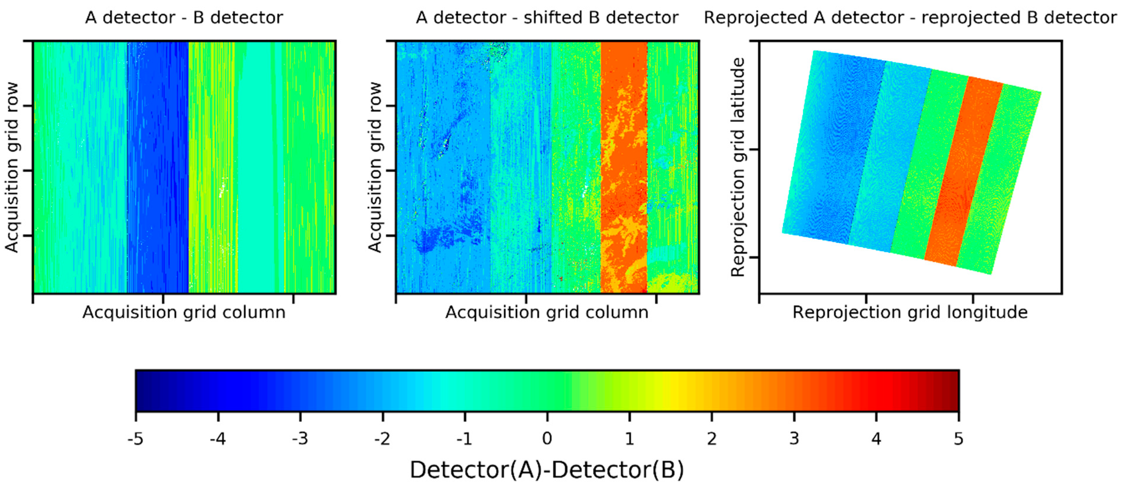
To do so, we use the 865 nm band (Oa17) which is the reference band for the geometric calibration. L1B TOA radiance images (three minutes granules) are converted to TOA reflectance images. The OLCI-A image is set as the reference product and remains fixed. Pixel-to-pixel spatial coregistration between OLCI-A and OLCI-B images is performed using macropixels of 5 × 5 pixels around each pixel taken as the centre. Proceeding per pixel of the OLCI-B image, the corresponding macropixel is shifted bidimensionally (+/−7 pixels allowed along-track (ALT) and/or across-track (ACT)). For each shift, a linear regression is computed between the OLCI-A reflectance and the OLCI-B reflectance from all pairs of pixels within the overlying OLCI-A and OLCI-B macropixels. The optimal shift (row and/or column shift) is the one giving the best correlation score, this is obtained when the ground targets are matched. Then, the optimal shifts act as a coregistration table to remap the OLCI-B product to the OLCI-A reference product, each OLCI-B pixel is moved to match the OLCI-A target. This is possible to do so only since OLCI-A and OLCI-B are on the same orbital track, pair images are nearly coincident.

It is most convenient to compare the images of the OLCI detector indices (“detector” hereafter) as the shifts are predominantly ACT after compensating an ALT offset between the two images, this offset is inherent of the splitting of the orbits into smaller portions (or “granules”) which are slightly translated between the two instruments. In Figure 2 (left and middle), we compare the differences between OLCI-A and OLCI-B detectors before and after shifting. We remark the striking differences, notably in cameras 1, 2, and 4. The detector differences are more inhomogeneous after applying the correlation shifts as the image correlation is performed using real images, which reveals the inhomogeneity of the target. For instance, cloud motion and parallax effects are prone to reduce the quality of estimating the optimal shifts. However, spatial inhomogeneities affect the detector differences to about +/−1 detector shift which roughly corresponds to the OLCI geolocation specification [1]. In both cases, there is no perfect correspondence between the detectors (i.e., no zero difference) as each camera of each sensor is not perfectly aligned. It is the role of geometric calibration to establish the correspondence between each camera (and each pixel ACT) and the ground.

In Figure 2 (right), we therefore show the differences between the detectors reprojected by means of the corresponding L1B geolocation of each sensor (right). This reprojection is uniform on a latitude/longitude grid and therefore the reprojection naturally reveals the orbital inclination of the sensors. Additionally, the decreasing size of the footprint from left to right (camera 1 to camera 5) reveals the tilted view of OLCI which sub-satellite point lies within camera 4.

The reprojected detectors (right image) map then correspond to the “shifted” differences (middle image) except slightly at the left border of camera 1 but with a difference of only one detector shift. This means that the L1B geolocation matches OLCI-A and OLCI-B as it independently matches each sensor with the ground. Moreover, the map of the differences between reprojected detectors (right) is more homogeneous due to the sole use of geometrical information, which shows that using reprojection is also preferable.

This image correlation analysis shows that the L1B geolocation (or at least the relative geolocation between OLCI-A and OLCI-B) is accurate. We therefore consider it safe to reproject the L1B products (radiances and any useful product) prior comparing pairs of products. We stress the need of also reprojecting the detectors of each sensor in order to make an accurate correspondence between L1B radiometry and the detector-dependent wavelength of acquisition. We now address this point.

4. Sensitivity Analyses and Homogenisation Methodology

In this section we investigate and adjust for spectral mismatches between OLCI-A and OLCI-B, which we denote by the term “homogenisation”. The process of homogenisation is that transformation of a sensor signal to a signal that corresponds to a nominal condition, or to a condition similar to the one of another sensor used for comparison. When restricted to spectral condition, such homogenisation process is known as spectral band adjustment (e.g., [9,10]). This process can be extended to differences in the geometry of acquisition, e.g., through knowledge of the target BRDF (e.g., [11]).

In the case of OLCI, homogenisation takes place at L1 processing for radiometric and geometric calibration and at L2 for spectral calibration (i.e., smile correction). This is because L1 products remain in radiance unit (which is the common unit for calibrated products) while the L2 processing starts by converting radiances into reflectances (which properties depend on the target) using the incoming solar irradiance convolved at the instrument spectral responses.

4.1. Spectral Misregistration Sensitivity Analysis

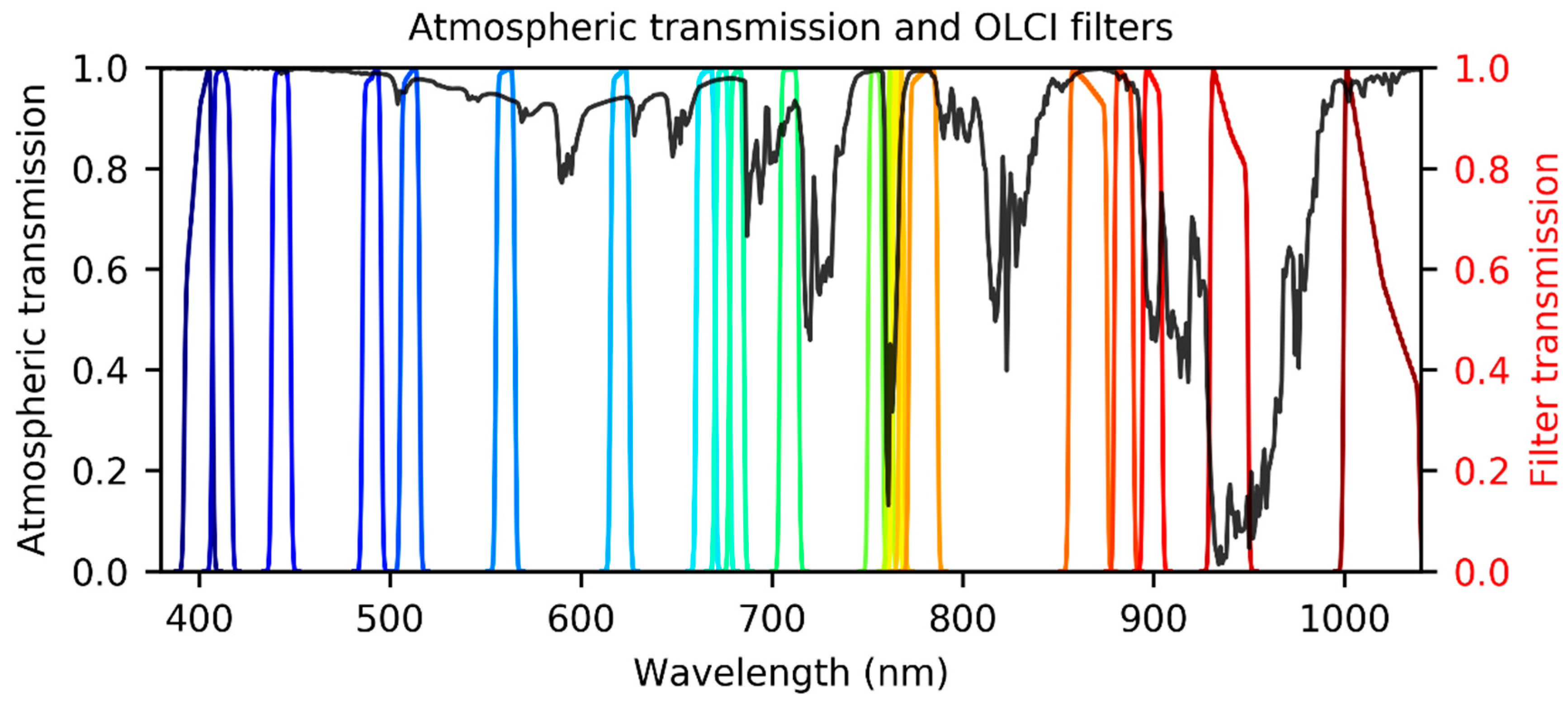
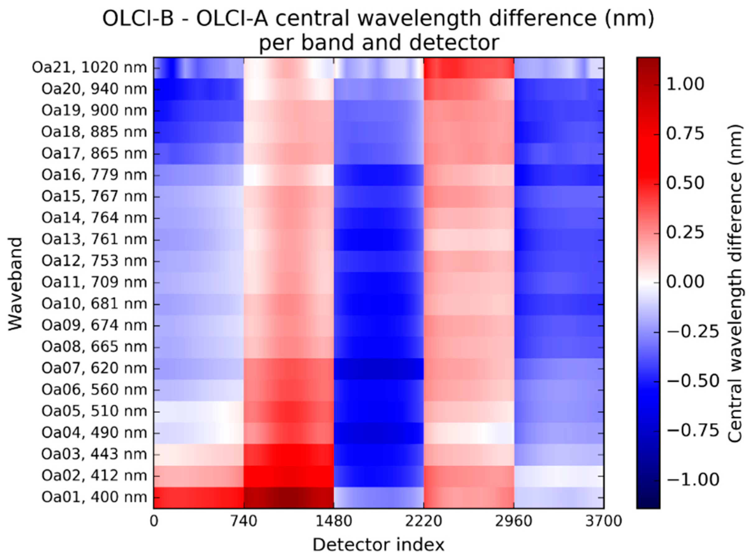
The OLCI spectral requirements drive the instrumental design to provide measurements at the nominal wavelengths detailed in Table 1 with a fine spectral resolution. By design, a spectrometer is subject to slight shifts of the wavelength of acquisition across the field-of-view, an effect called “smile” (see [12] for MERIS). Spectral characterisations of OLCI-A and OLCI-B exhibit small differences as shown in Figure 3 (absolute values for both sensors) for bands Oa01 and Oa17 (all other bands providing qualitative similarities) and (differences between the two sensors) in Figure 4 for all bands per detector. Data from each camera of 740 detectors is aggregated to the previous and succeeding ones (if any) using a continuous detector index. At 400 nm, the differences are the strongest with up to about 1 nm difference in camera 2.

4.1.1. Sensitivity of Radiance-to-Reflectance Normalisation to Solar Irradiance Differences

Even such small shifts can have a significant impact on the top-of-atmosphere radiance (or “measurand”, using metrological terminology): the two sensors do not measure exactly the same radiance as they do not measure radiance at exactly the same wavelength. Although the natural unit for calibration is radiance (and is the unit provided up to L1B products) it is more relevant for passive remote sensing in the solar range (from Ultra-violet to Shortwave-infrared) to analyse the collected signals in reflectance unit, reflectance being a property of the target. The radiance-to-reflectance conversion handles the normalisation of the upcoming radiance arising from the target to the sensor by the incoming solar illumination received by the target and convolved with the instrument spectral response function. In the radiance-to-reflectance formulation the radiance $L\left(\lambda \right)$ is converted to the reflectance $\rho \left(\lambda \right)$ through

$$\rho \left(\lambda \right)=\frac{\pi L\left(\lambda \right)d^2}{F_0\left(\lambda \right)\cos {\theta }_s}$$

(1)

The solar illumination $F_0\left(\lambda \right)$ is scaled by the solar zenith angle ${\theta }_s$ seen by the target (0° corresponding to maximum illumination with Sun at zenith) and $d^2$ the Earth-Sun distance in astronominal units. $F_0\left(\lambda \right)$ is taken from Thuillier [13] and its convolution with the Instrument Spectral Response Function (ISRF) is performed from the spectral characterisation per detector and included in each L1B product. The conversion to reflectance is coherent with the absolute calibration methodology which uses a reflectance reference.

Based on this conversion, the first discrepancies between the two OLCI sensors radiometry arise from the different ISRFs and the corresponding solar illumination factors. Let us consider one OLCI channel with ${\lambda }_0$ its nominal wavelength. Let ${\lambda }_{i,A}$ and ${\lambda }_{j,B}$ be the wavebands corresponding to the detector index $i$ (resp. j) of OLCI-A (resp. OLCI-B). Due to the slight geometrical misregistrations, tandem acquisitions do not necessarily match i and j over the same target, though these are close to about +/−5 maximal departure. For this exercise we however assume that $i=j$, a difference of 5 detectors, indeed causes a maximal wavelength shift about 0.01 nm and its impact is negligible compared to a maximal 1 nm shift considered here between OLCI-A and OLCI-B.

The ratio $r_L$ of the radiances, induced by the spectral shift between OLCI-A and OLCI-B, expresses as

$$r_L=\frac{L_B\left({\lambda }_{i,B}\right)}{L_A\left({\lambda }_{i,A}\right)}$$

(2)

which, for a “perfect” target having constant reflectance (e.g., a cloudy surface) observed in the same acquisition conditions and without any disturbance from the atmosphere (i.e., no absorption, emission, nor scattering), translates into the ratio between the solar illumination factors:

$$r_L\left(\rho \left(\lambda \right)=cst\right)=\frac{F_0\left({\lambda }_{i,A}\right)}{F_0\left({\lambda }_{i,B}\right)}$$

(3)

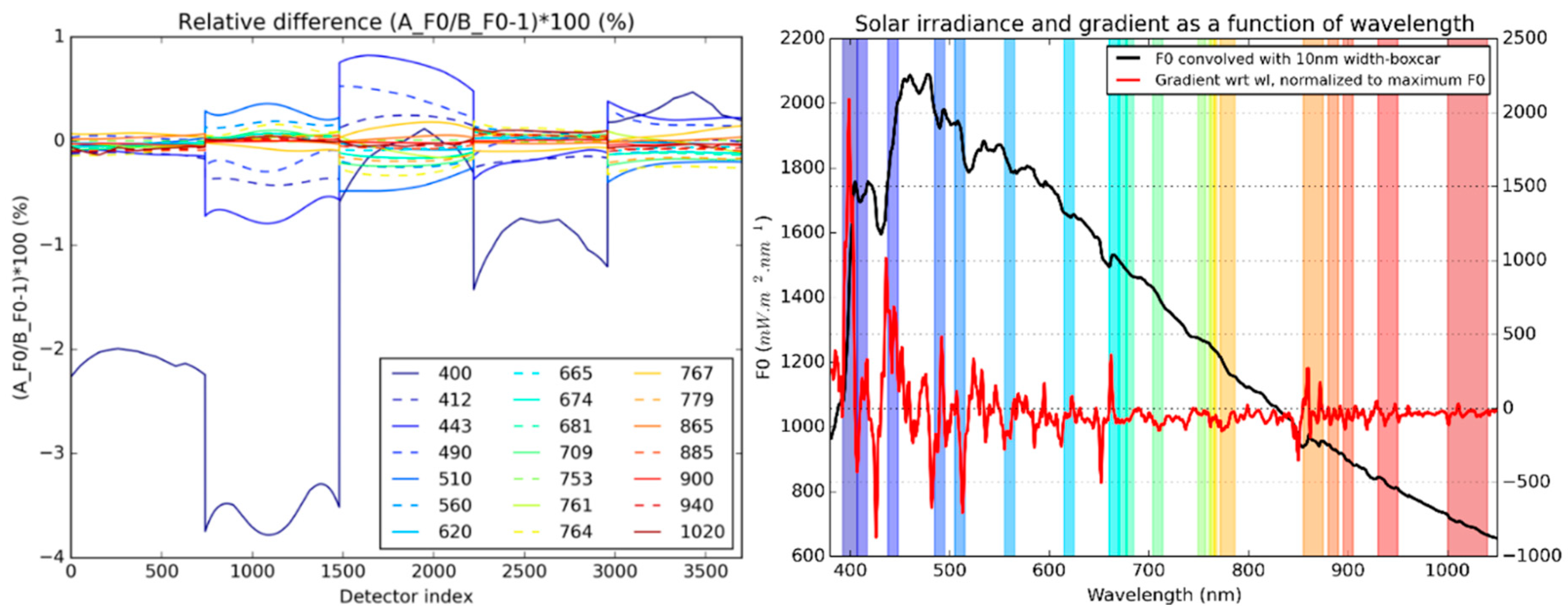
Figure 5 shows this ratio (left), expressed in percent $\left(r_L-1\right)\times 100\%$, as a function of the detector index, for all OLCI bands. This represents the biases induced by comparing OLCI-A and OLCI-B radiometry in radiance unit (i.e., band per band without considering the spectral characterisation) rather than in reflectance unit or in spectrally-adjusted radiance. As we can see, a 1 nm difference causes up to nearly 4% difference at 400 nm, less as we progress from blue to red. This is due to the strongest gradient in the solar illumination factor in the UV-blue spectral region [13]. Notably, the effect at 412 nm (Oa02) is much decreased compared to 400 nm (Oa01). In Figure 5 (right), we have convolved the solar irradiance from [13] with a 10 nm boxcar filter (black line) and computed the gradient with respect to wavelength (red line). This clearly shows that the 400 nm band lies at a position of steepest gradient. It is therefore mandatory to assess comparisons between the two sensors in reflectance unit or to adjust the radiance for the difference in ISRFs (i.e., compute spectrally-adjusted radiance).

Further adjustment of the reflectance is also necessary to compensate for gaseous absorption and Rayleigh scattering as analysed below.

4.1.2. Sensitivity of Reflectance to Gaseous Absorption and Rayleigh Scattering

After conversion to reflectance, ${\rho }_A\left({\lambda }_{i,A}\right)$ and ${\rho }_B\left({\lambda }_{i,B}\right)$ must be adjusted through the procedure known as smile correction. In the nominal OLCI L2 processing, this processing step aims at shifting the TOA reflectance from each detector waveband to the corresponding nominal (central) OLCI waveband. It is performed using assumptions on the signal composition and spectral dependency.

The most impacting physical factors are gaseous transmittance and molecular scattering (mostly Rayleigh scattering). Gaseous transmittance is first used to correct for the direct absorption of the atmospheric gases such as water vapour (H₂O), oxygen (O₂), ozone (O₃), and nitrogen dioxyde (NO₂) which are accounted for in the nominal OLCI L2 processing. The total gaseous transmittance is the product of each transmittance, acting over the OLCI spectral range.

$$T_{gas}\left(\lambda \right)=T_{H_{2}O}\left(\lambda \right)\times T_{N{O}_2}\left(\lambda \right)\times T_{O_3}\left(\lambda \right)\times T_{O_2}\left(\lambda \right)$$

(4)

Following the assumptions of the OLCI L2 processing, only strong absorption features (O₂ and H₂O absorption) exhibit significant changes with respect to small spectral shifts so that the total transmittance shall write

$$T_{gas}\left({\lambda }_{i,A}\right)=T_{H_{2}O}\left({\lambda }_{i,A}\right)\times T_{N{O}_2}\left({\lambda }_0\right)\times T_{O_3}\left({\lambda }_0\right)\times T_{O_2}\left({\lambda }_{i,A}\right)$$

(5)

(and resp. for ${\mathit{\lambda }}_{\mathit{j},\mathit{B}}$).

We do not try to adjust for these effects as we do not possess the tools to accurately model the corresponding fine spectral features in the strong absorption bands Oa13, 14, 15 (O₂ bands), and Oa19 and 20 (H₂O bands). Moreover, absorption is strongly sensitive to the gaseous contents which knowledge probably requires high accuracy for our purpose.

Total transmittance relates the TOA reflectance to the so-called “gas-corrected” reflectance (termed “ng” for “no gas” in the OLCI L2 processing) through

$${\rho }_{TOA}\left({\lambda }_{i,A}\right)=T_{gas}\left({\lambda }_{i,A}\right)\times {\rho }_{ng}\left({\lambda }_{i,A}\right)$$

(6)

Finally, smile correction adjusts this gas-corrected signal to the OLCI nominal wavebands, across the complete field-of-view (FOV). It is performed in two steps: first by adjusting the Rayleigh scattering spectral dependency, then by adjusting the residual ground signal spectral dependency after Rayleigh correction (i.e., after removal of the contribution due to Rayleigh scattering).

The sensitivity of the Rayleigh scattering contribution can be estimated from the radiative transfer models used in the OLCI L2 processing. We base our example on two extreme cases: one with the small scattering contribution with solar and viewing zenith angles about 30° and opposite azimuths, one with large scattering contribution with equal and high solar and viewing zenith angles and coincident azimuths (i.e., backscattering conditions with large airmass).

Using the same notations as above, a Rayleigh scattering change $\Delta {\rho }_{ray}$ according to the spectral shift ${\lambda }_{i,A}-{\lambda }_{i,B}$ can be estimated as

$$\Delta {\rho }_{ray}=\left(\frac{\partial {\rho }_{ray}}{\partial \lambda }\left({\lambda }_0\right)\right)\left({\lambda }_{i,A}-{\lambda }_{i,B}\right)$$

(7)

Such change does not have the same impact depending on the composition of the TOA signal of the target. The impact is largest over open oceans where Rayleigh scattering represents up to 90% of the signal. An estimation of the relative impact can thus be performed as $\Delta {\rho }_{ray}/{\rho }_{ray}\left({\lambda }_0\right)$ expressed in Figure 6 in percent for each of the two cases.

The relative differences are higher for the small Rayleigh scattering values (left figure). The impact is the large in the blue and upper bounded by about 1% in camera 2 in the worst case, roughly lower than 0.3% in general. These factors are computed to provide a view of the relative error made by not considering the Rayleigh adjustment. These show that solar irradiance and Rayleigh adjustments can either have concomitant or opposite impacts, especially in the blue where $F_0\left(\lambda \right)$ has a steep gradient at 400 nm which then decreases and inverts at about 500 nm.

4.1.3. Conclusion of the Sensitivity Analyses

In conclusion, these analyses show that it is mandatory to homogenise the datasets, i.e., to adjust the measurand, prior assessing comparisons between two sensors with close, yet different, ISRFs. Even the tiniest spectral differences can have a large impact, especially in the blue spectral region. Considering TOA radiance instead of TOA reflectance can cause up to 4% systematic bias due to the strong sensitivity of the solar irradiance factor to the wavelength of acquisition. Spectral dependency of the Rayleigh scattering can cause up to a 1% bias.

This means that smile-corrected reflectance must much preferably be (and are) used to compare the radiometry of the two sensors. Where Rayleigh scattering is less efficient (mostly above middle to high clouds), reflectance however suffices. Homogenised reflectance then refers either to smile-corrected reflectance or to reflectance when only radiance-to-reflectance conversion is performed.

4.2. Homogenisation Methodology and Validation on a Single Scene

Smile-corrected reflectances are not provided in the nominal OLCI products (neither L1B nor L2). To overcome these issues, we have built a breadboard of the OLCI L2 operational smile-correction algorithm starting from L1B products. Smile-correction is disabled over clouds as these carefully selected targets are white. This breadboard directly uses reprojected L1B products as input, which is much handier for the analysis as we do not need to reproject all parameters to be analysed if taking the original inputs in initial format. We recall that reprojection is necessary to handle slight spatial misregistrations between the two instruments.

Two options can then produce homogenised datasets of OLCI-A and OLCI-B dedicated to our analysis. The first option considers aligning spectrally one sensor to the other (i.e., aligning OLCI-A toward OLCI-B, termed “A2B” or aligning OLCI-B toward OLCI-A, termed “B2A”). This can be done by considering only the detector-dependent spectral shifts to adjust one OLCI instrument to the other. It also has the advantage of performing only one adjustment for the analysis, which is less computationally demanding. The other option is to align both OLCI-A and OLCI-B toward the same nominal reference (termed “A2N” and “B2N”) as is done in the nominal L2 processing. Although smile-correction must be processed twice, we prefer to choose this option for compatibility with the nominal L2 processing.

To summarize the homogenisation process, we sketch below the steps for both OLCI-A and OLCI-B to adjust the measurand to a reflectance measured at the nominal wavelength ${\lambda }_0$:

$$L_A\left({\lambda }_{i,A}\right)=L_A^{TOA}\left({\lambda }_{i,A}\right) \stackrel{F_0\left({\lambda }_{i,A}\right)}{\Rightarrow }{\rho }_A\left({\lambda }_{i,A}\right)={\rho }_A^{TOA}\left({\lambda }_{i,A}\right)\stackrel{T_{gas}\left({\lambda }_0\right)}{\Rightarrow }{\rho }_A^{ng}\left({\lambda }_{i,A}\right)\stackrel{SC\left(A2N\right)}{\Rightarrow }{\rho }_A^{sc}\left({\lambda }_0\right)$$

(8)

$$L_B\left({\lambda }_{j,B}\right)=L_B^{TOA}\left({\lambda }_{j,B}\right) \stackrel{F_0\left({\lambda }_{j,B}\right)}{\Rightarrow }{\rho }_B\left({\lambda }_{j,B}\right)={\rho }_B^{TOA}\left({\lambda }_{j,B}\right)\stackrel{T_{gas}\left({\lambda }_0\right)}{\Rightarrow }{\rho }_B^{ng}\left({\lambda }_{j,B}\right)\stackrel{SC\left(B2N\right)}{\Rightarrow }{\rho }_B^{sc}\left({\lambda }_0\right)$$

(9)

${\mathit{\rho }}_{\mathit{A}}^{\mathit{s}\mathit{c}}\left({\mathit{\lambda }}_{\mathbf{0}}\right)$ and ${\mathit{\rho }}_{\mathit{B}}^{\mathit{s}\mathit{c}}\left({\mathit{\lambda }}_{\mathbf{0}}\right)$ are the homogenised (i.e., smile- and gas-corrected TOA reflectances) that must be used preferably to compare OLCI-A and OLCI-B radiometry. Except in strong absorption bands, gas-correction is not much sensitive to the slight spectral differences between the two sensors (the nominal L2 processing indeed does not consider spectral dependency of the gaseous transmission) and is computed directly at the nominal wavelength.

It must be recalled that smile-correction is performed in the first steps of the OLCI L2 operational processing to provide a homogeneous baseline for the atmospheric corrections. It is also at this level of processing that system vicarious calibration for the water processing branch is evaluated and applied.

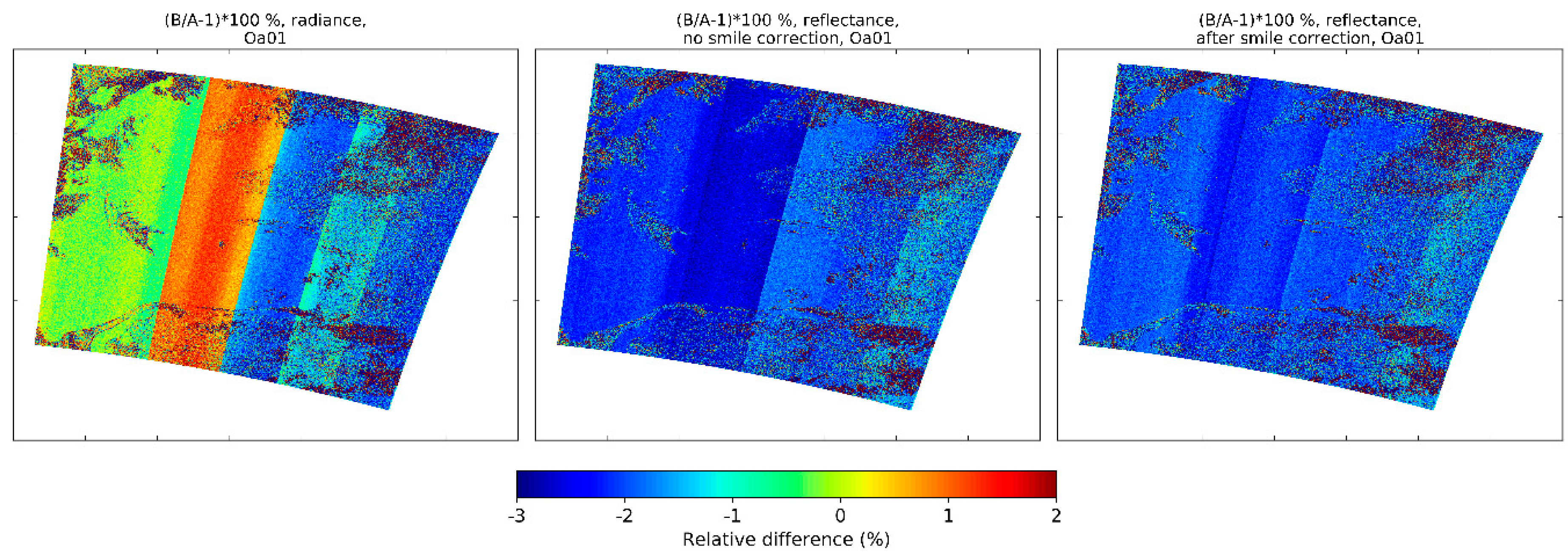
First differences between OLCI-A and OLCI-B radiometers are shown in Figure 7 at Oa01 (400 nm) where sensitivity in spectral differences is the highest. Radiance differences (left) are the most striking with up to +/−2% differences due to the strong sensitivity of the solar irradiance in this channel. As expected, conversion to reflectance (middle) drastically reduces these differences.

At camera 2, where the spectral differences are the largest between OLCI-A and OLCI-B, the smile-correction further compensates the differences remaining after radiance-to-reflectance conversion (about 0.5%) which are mostly due to the Rayleigh scattering spectral dependency (right of Figure 7). Overall, the smile-corrected reflectance then seems more homogeneous. Remaining differences appear within and between the cameras and are investigated in more details in Section 5.

4.3. Target Classification

Cloudy, land, and water targets have different spectral and spatial properties and are more or less sensitive to the underlying assumptions used in the spatial and spectral adjustments necessary to cross-compare the measurements. Therefore, it is much useful to separate these targets in the analysis as they potentially provide different results (e.g., [10]). These targets are classified from the L1 processing which uses the geolocation combined to an auxiliary atlas for water/land discrimination, and radiometric thresholds for the detection of the brightest cloudy pixels. For water pixels we exclude pixels affected by sun-glint, this has proven to be very efficient in the quality of the results (not shown).

The clouds are further distinguished to select clouds above which Rayleigh correction can be neglected. These are selected using a threshold on the reflectance in the strongest oxygen absorption band Oa13 (761.25 nm). A sensitivity analysis (not shown) led to consider reflectances higher than 0.2.

Whereas land targets are predominantly green, a subselection of desert targets over the Sahara (longitudes between 20°W and 60°E, latitudes between 15°N and 35°N) provides a last category termed “deserts”, distinguished from “land” targets which comprise all kinds of ground targets. Indeed, deserts provide bright targets with a spectral signature different to the one of vegetated areas.

In the next section, we then distinguish between land (all types), water (sun-glint free), selected clouds, and desert. Only pixels which belong to the same target class for OLCI-A and OLCI-B are considered.

5. Cross-Comparisons, Harmonisation, Validation of the Approach

In this section, we apply the homogenisation methodology on the extended tandem dataset and investigate the relationships between OLCI-A and OLCI-B in close details. Daily statistics provide the basis of the analysis, from which convergence is obtained rapidly over any comparison target. Persistent biases between the two sensors are found to be stable over time with decreasing bias along the OLCI spectrum (from blue to NIR). Choice is justified for selecting clouds as preferable targets to provide harmonisation coefficients which are then used to process a dedicated reprocessing of datasets where OLCI-A is aligned radiometrically on OLCI-B. The approach is validated and shows the excellent alignment of the two sensors.

5.1. One Day Analysis of OLCI-A vs. OLCI-B for All Targets

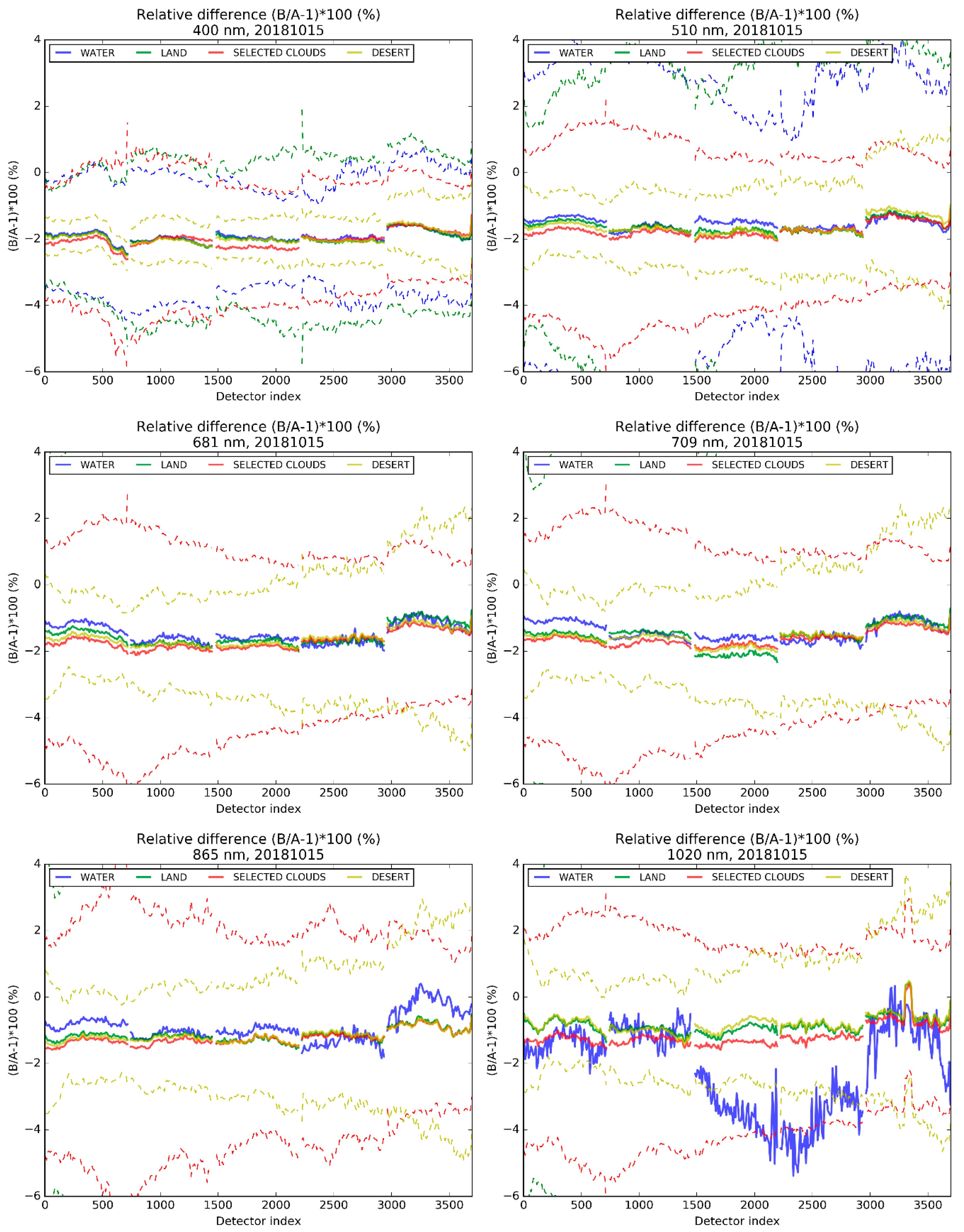
From the tandem data archive, we process the homogenisation methodology over a few orbits of OLCI-A and OLCI-B acquisitions on 15 October 2018. The last tandem date available is chosen here as it exhibits the most stable results for Oa01 which calibration is slightly affected by the efficiency of the temporal degradation model in camera 3 (not shown). We proceed to a statistical analysis, separating water, land, selected cloud, and desert targets. A huge database is aggregated and consists of tens of millions of pairs of pixels. Comparisons are based on the relative differences between the homogenised TOA reflectances rather than on the absolute differences. Indeed, those differences are found more stable than the absolute differences (not shown).

Results are shown in Figure 8 for a reduced and selected set of bands (Oa01, Oa05, Oa10, Oa11, Oa17, Oa21), full results are provided in supplement Figures S1–S4. Results over strong gaseous absorption bands (Oa13, Oa14, Oa15, Oa19, and Oa20) are only presented there for the sake of completeness. These are not meant to be used for research since finer gaseous transmission corrections must be applied for valid comparisons. They however provide indication of the effects of the spectral differences between the two sensors.

Relative differences $\left(\frac{{\rho }_B\left({\lambda }_0,i\right)}{{\rho }_A\left({\lambda }_0,i\right)}-1\right)\times 100$% at wavelength ${\lambda }_0$ are shown per bin of ten detectors (i referring to the central detector value) across the complete FOV. This averaging is performed to reduce noise and speed up the analysis without damaging the results. For each detector bin, median (plain line) and median absolute dispersion (dashed lines indicating median +/− dispersion) are computed for each target. Medians are preferred to means since the latter are sometimes affected by outliers (e.g., occurring through saturated pixels in one or the other sensor). Values are reported for water, land, selected clouds, and desert, respectively in blue, green, red, and yellow. This allows to underline benefits and drawbacks of using each category as highlighted in the following.

The scale is kept between −6% and 4% for the sake of legibility (−20% to 10% for the O₂ bands) although the dispersion is usually off the scale. Tiny gaps are visible ACT corresponding to the overlap regions of the OLCI cameras (every 740 detectors): about 30 detectors for each adjacent camera share a common footprint area at each camera interface. Gaps in the results correspond to the missing detectors in the image resulting in the constant selection of one camera at each interface. Missing this information is not impacting our conclusions as those pixels will never be used in the nominal OLCI processing.

These results show that the tandem analysis provides an excellent precision for cross-sensor radiometric comparisons (notably compared to the Landsat tandem results of Teillet [10]), reaching details lower than 0.5% differences across the complete Field of View (FOV). What is most obvious is a consistent bias between the two sensors, OLCI-A being brighter than OLCI-B from about 2% in the blue to about 1% in the NIR. The reason of this is unclear but we suspect such biases can originate from the pre-flight characterisation of the diffusers (which is challenging to achieve). This can be justified by considering that all processings are common to both sensors whereas the absolute calibration only relies on the independent pre-flight characterisation of the diffusers.

Over water, the comparisons no longer hold at wavelengths higher than 865 nm where the signal is too weak due to the absorption of light by water. At the first bands, dispersion from results over all targets is of the same order of magnitude except over deserts where it is lower due to the homogeneity of the target. However, mixed pixels (e.g., including small clouds not tagged as bright) may be included in the land and water statistics and provide a widening of the dispersion. Clouds provide the most consistent dispersion over all channels and remain relatively low, which means that the strength of the signal as well as the whiteness of the target compensate the drawbacks of potential cloud motion and parallax.

It is to be noted that the statistics being provided by millions of datapoints, the computation of the standard error (i.e., the standard deviation divided by the square-root of the number of datapoints) is not provided in the figures because it leads to near zero uncertainty. This means that the statistical convergence of the results is ideally high and allows to reach details lower than 0.5% across the complete FOV. In other words, it also means that the differences shown between results over the different targets are due to modelling errors and/or instrumental artefacts rather than by noise. Compared to cross-calibration of sensors from different payloads, where the number of comparison points is much smaller, that same notion of precision can be interpreted differently. For instance, based on simultaneous nadir overpasses, [14] show that VIIRS VNIR bands agree with MODIS within 2% with bias uncertainty less than 1%. In our analyses, from a tandem configuration, such bias uncertainty is reduced to near zero.

Inter-camera differences are seen at all bands with similar features. As all cameras are physically independent optical systems, calibration residuals can persist either on OLCI-A, OLCI-B, or both sensors for any of the camera. This will be further discussed in the discussion section.

Intra-camera “hat-shaped” features also persist at all bands for all cameras with similar shapes for all bands within a given camera. Their proportions (maximum about 0.5%, usually about 0.2%) are smaller than the inter-camera differences (between 0.5% and 1% between cameras 4 and 5). These differences are likely to be due to deficiencies in the straylight correction algorithm and are similar for both sensor and each camera individually. The interband monitoring of Deep Convective Clouds (DCC) observations highlight such artefacts, individually for each sensor, when the proportions of these effects strongly vary from one band to another or when the two bands are spectrally far enough (see, for instance [15], for more details on interband monitoring from DCC observations). In Figure 9 for OLCI-A (left) and OLCI-B (right), ratios between the reflectance at 779 nm and the reflectance at 560 nm (used as reference) over DCC observations which indeed betray intra-cameras calibration residuals impacting each of the two bands individually. These features cannot be due to clouds BRDF effects since, from one side of the FOV to the other, the viewing angle is continuously changing and since solar illumination angles are (on average) smoothly changing. BRDF effects appear rather in the slight trend of the interband ratios across the FOV.

Finally, a much specific artefact appears in the comparisons at Oa21 (1020 nm) in an isolated region of the camera 5, around detectors 3200 to 3300 (see again Figure 8). A spike in the relationships provides evidence that one of the sensors is affected by an anomaly. This was known from the analysis of the OLCI-A radiometric in-flight calibration data [16], and from the evolution with time of the anomaly, attributed to the presence of a manufacturing droplet contaminant. The question, however, of the location of the droplet, either on the solar diffuser or inside the instrument optical path, was not solved until the tandem data analysis allows to conclude that such a tiny effect (1%) is strictly originating from the detection chain.

Regarding the different targets, results perfectly match at camera 4 where the geometry is most favourable (smallest viewing angles, including sub-satellite point, and small spectral differences), except over water at wavelengths higher than 681 nm and over land at 1020 nm.

Except for camera 4, results show differences between target classes, with sometimes about 0.5% and up to 1% maximum discrepancies. These differences are not directly explained by differences in the instrument spectral responses (not shown). There is neither evidence of an impact of the assumption of using spectrally-independent gaseous transmission within the A or B wavebands (excluding for strong gaseous absorption bands) since an impact would be evident on all cameras.

Camera 3 shows the strongest disagreements with results over land coping either with results over water (e.g., Oa02) or with results over clouds (e.g., Oa05). This is remarkable as this camera does not provide too high viewing angles. The OLCI-A and OLCI-B spectral differences are quite significant in this camera but sometimes as significant as in camera 2 where comparisons are much more stable between targets. At 709 nm over land, there seems to be a mishandling of the spectral adjustment in the vegetation red edge, where reflectance has a specific strong spectral-dependency (e.g., [17,18]). The variation of the intercalibration gains ACT is indeed not continuous in this waveband.

In conclusion, intercomparisons over selected clouds and deserts provide the best results with lower dispersion and best spectral consistency. This corroborates the use of such targets for radiometric validation and vicarious calibration (e.g., [19,20]). Despite a lower spatial coverage (within a day, only two or three OLCI, 3-min, granules cover the Sahara region), results over deserts provide the least dispersion. However, results over selected clouds are much more consistent spectrally as these targets do not require a spectral adjustment. We therefore preferably rely on the results over selected clouds.

Depending on the time-separation between the two payloads this conclusion may however be subject to change. Indeed, a 30 s delay between Sentinel-3 OLCI observations of 300m spatial resolution does not lead to significant changes in the cloud patterns while a longer tandem separation (e.g., few minutes) would probably severely restrict the analysis at 300m spatial resolution (for example, the ESA FLEX tandem separation from Sentinel-3 OLCI is planned for ~10 s since the spatial resolution of FLEX is 280 m [21]). The use of desert areas then becomes preferable as those targets are much more stable. When the delay becomes too large, differences in the solar illumination angle must however be compensated.

5.2. Analysis Over the Full Tandem Phase: Temporal Stability

Following the above, we conduct the same analyses, independently over each available date of the tandem phase datasets (i.e., on a weekly basis, each Monday). The temporal stability of the inter-calibration coefficients is assessed, per target, through statistics per band and per camera as any camera can evolve over time independently to each other, spectrally and/or radiometrically.

First, differences between the gains obtained at the last (25 June 2018) and the first (15 October 2018) dates available provide information on the stability of the coefficients over the duration of the tandem phase, mean and dispersion of the gain differences (last date ones minus first date ones) are computed over all detectors. Second, the collection of all the gains (independently retrieved for each day of the data archive) allows to derive minimal, mean, and maximal values of the standard deviations obtained from each detector over the time. Results are shown in Figure 10 for (e.g.,) camera 3, results for all cameras are displayed in supplement Figures S5 and S6.

On the left figures, the differences between last and first dates show that the gains are temporally stable to within 0.2% in absolute to the exclusion of water targets from red to NIR and land targets in the red edge (681 and 709 nm), to that respect all cameras do not respond equally. Results over clouds and deserts are mostly below 0.1% in absolute, rarely close to 0.2%.

On the right figures, mean standard deviations are between 0.02% and 0.1% for all targets, usually better for land and water targets in the blue-green region, worse over water in the NIR, consistent with previous observations. Over land, results degrade in the red edge. Over clouds and deserts the results are very stable spectrally for each camera and remains between 0.03% and 0.07% for all cameras.

All these results highlight that clouds and desert provide the most stable and consistent results for the intercalibration of the two sensors. As stated in the preceding section, results over clouds are trusted with more confidence. Clouds behave similarly to on-board diffusers, they even can be considered as a common “statistical diffuser” for the two sensors. We therefore make the choice of using results from these targets as the reference for the harmonisation of OLCI-A and OLCI-B.

5.3. Harmonisation

The harmonisation (here to be understood as a radiometric alignment) of OLCI-A and OLCI-B is based on the results obtained from the measurements from 15 October 2018, over the selected clouds. The rationale for such choice (one date) is to select one specific date at which the relationships between the two sensors are considered most stable, rather than a longer period. This eases the process of recalibration, if necessary, as absolute calibration gains (independently for OLCI-A and OLCI-B) have temporal dependency.

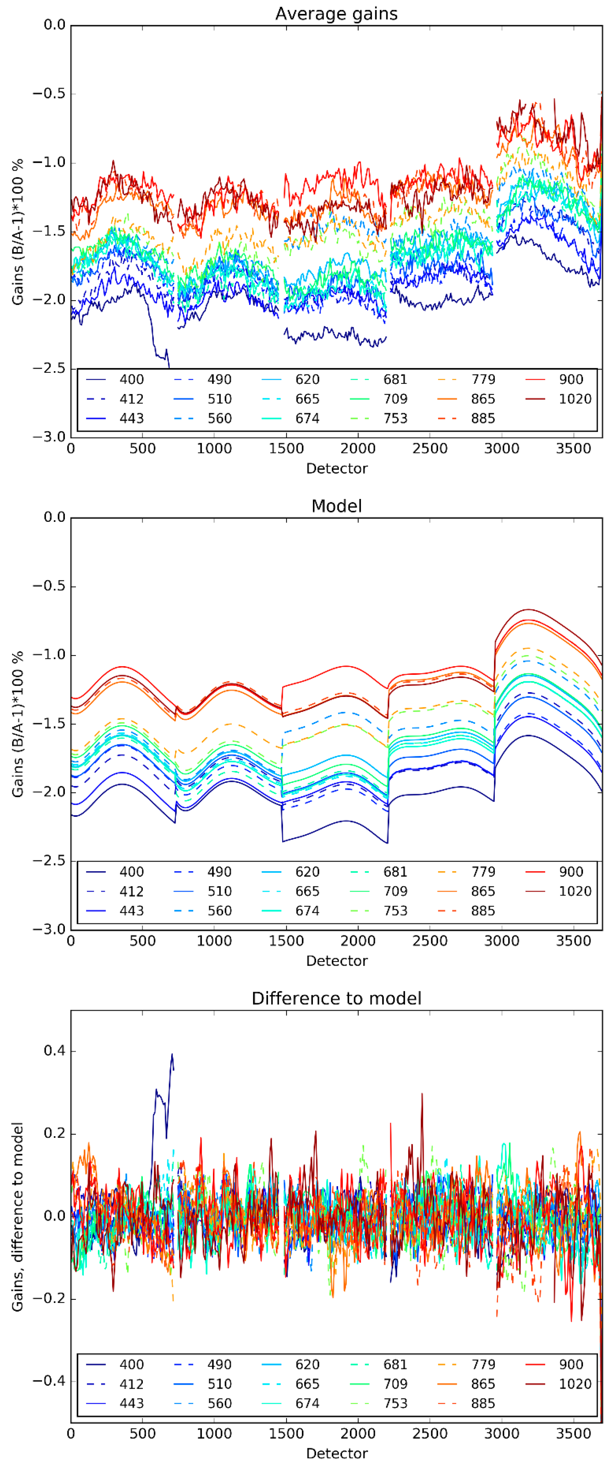
The obtained average ACT-profile is shown in Figure 11 for all bands (to the exception of strong absorption bands). It exhibits very similar “hat-shaped” features for each camera at all bands, a clear “rainbow effect” also appears from blue to red highlighting the decreasing bias with increasing wavelength. According to the OLCI calibration team, there is no clear evidence of the root cause of the inter-instrument biases and their spectral signature. However, as the whole processing chain, from ground characterisation to EO data processing, is common, it seems justified to suspect such biases can origin from the pre-flight characterisation of the diffusers bidirectional reflectance functions.

Given these observations, we model, for each camera, intercalibration gains as the sum of a mean bias per band (spectral dimension only) and an average shape (spatial dimension only) built from all bands. The average shape is fitted using a polynomial (order 5 being enough). The computation is performed for all bands excepting the strong absorption bands which models are linearly interpolated from the ones of the other bands. The anomalous spike at camera 5 for Oa20 is also removed from the computation as well as the outlying values of the very eastern edge of the swath. The average gain ACT-profile, the fit, as well as the residual errors are also shown in Figure 11.

Although considered with less reliability, the average ACT-profiles from the other targets can be obtained similarly. The residual errors between the clouds model of Figure 11 and these averages are shown in the supplement Figure S7. Residuals over clouds of Figure 11 is reproduced for comparison at the same scale. There, the anomalous spike at Oa20 is kept. For water targets, where most useful bands are in the blue-green region, residuals of +/−0.5% persist with variability between cameras which may be caused by non-linearity issues at low radiances. For land targets, about 0 to 0.5% bias is also shown with stronger discrepancies in the red-edge (especially 709 nm where the reflectance gradient is the highest). For deserts, the residuals are similar to the ones over land, without the spectral discontinuity in the red-edge. These observations are in line with the differences of Figure 8 (also supplement Figures S1–S4). Further investigations are necessary to propagate these differences at L1 into differences in the L2 products and are the subject of the companion paper [5].

Harmonisation then proceeds by applying the modelled coefficients (more precisely the ratios B/A converted from these relative differences) at L1 radiance to align one sensor on the other. Many radiometric validation assessments provide evidence that OLCI-A is too bright, while OLCI-B agrees better with other missions and simulations [4]. For this reason, we choose to align OLCI-A on OLCI-B for the validation of this approach. For future Sentinel-3C and Sentinel-3D OLCI sensors, the approach will need to be re-evaluated depending on the relative performances of each sensor at that time.

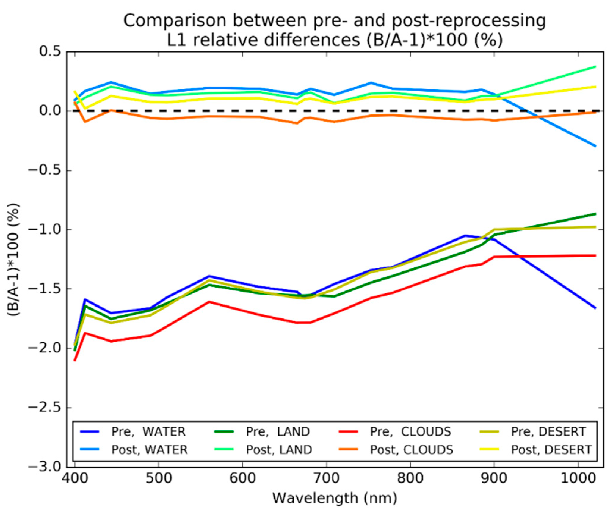
5.4. Validation of the Harmonisation: Post-Reprocessing Comparisons

For validation purposes, a custom reprocessing has been performed over few dates of the tandem and drift periods (6, 13, 20 and 27 August, 3, 10, 17 and 24 September, 22 and 29 October, and 3, 10, 17 and 24 December). L1 and corresponding L2 products have been generated using the same processing software as the operational processing chains but employing specific custom calibration gains for OLCI-A accounting for the alignment to OLCI-B. This is performed directly by multiplying the nominal OLCI-A calibration gains by the harmonisation factors. We recall that the harmonisation factors are taken from the statistics of one day of tandem data (15 October 2018) over selected clouds.

With respect to L1 radiance products, we stress that it is erroneous to think that the harmonisation process leads to comparable radiance products as the two OLCI sensors measure TOA radiances at slightly different wavelengths whichever radiometric calibration is applied. Therefore, as understood from the preceding sections of this paper, the post-reprocessing comparisons must again be made on smile-corrected L1 reflectances. We do so by performing the same adjustments as in the preceding sections.

Computations are done for data acquired on 24 September 2018, which is the latest in the tandem which is common to both pre- and post-reprocessing datasets. For the sake of brevity, we compute the mean statistics over all the data (regardless of the camera) and compare pre- and post-reprocessing results. Individual results per target are compared in Figure 12, absorbing bands are not considered.

Clearly, the radiometry of both sensors is now very well aligned. The decrease of the bias with increasing wavelength has been mitigated and all median differences are within 0.25% (except at 1020 nm over water and land where it remains below 0.4%). These results are of excellent precision for cross-sensor calibration, showing the efficiency of a tandem phase at early phase of a mission. To maintain the climate record, it is highly recommended that the future Sentinel-3C and Sentinel-3D satellites perform tandem flights when injected into the Sentinel-3 time series.

However, these results are relative of one sensor against the other, which again raises the question of the reference to use. This is all the more of interest as all cameras do not compare equally, there is suspicion that one or both sensors are not well equalized with respect to the cameras. This is further discussed in the next section.

6. Discussion: The Question of the Reference Sensor

The radiometric alignment of OLCI-A on OLCI-B is proved to be effective with median residual errors smaller than 0.3% in absolute, which is excellent to ensure mission continuity for the OLCI program. However, a question remains on the reference to use for an OLCI “system of system” calibration set-up, especially as the relationships between OLCI-A and OLCI-B exhibits camera dependencies (notably between camera 4 and 5). In the lack of an absolute, independent, reference, we miss the information of which sensor(s) is (are) responsible for these inter-camera differences and to which extent. Would one sensor be aligned to the other in an operational setting, we must be sure on the relevance of the sensor being chosen as reference.

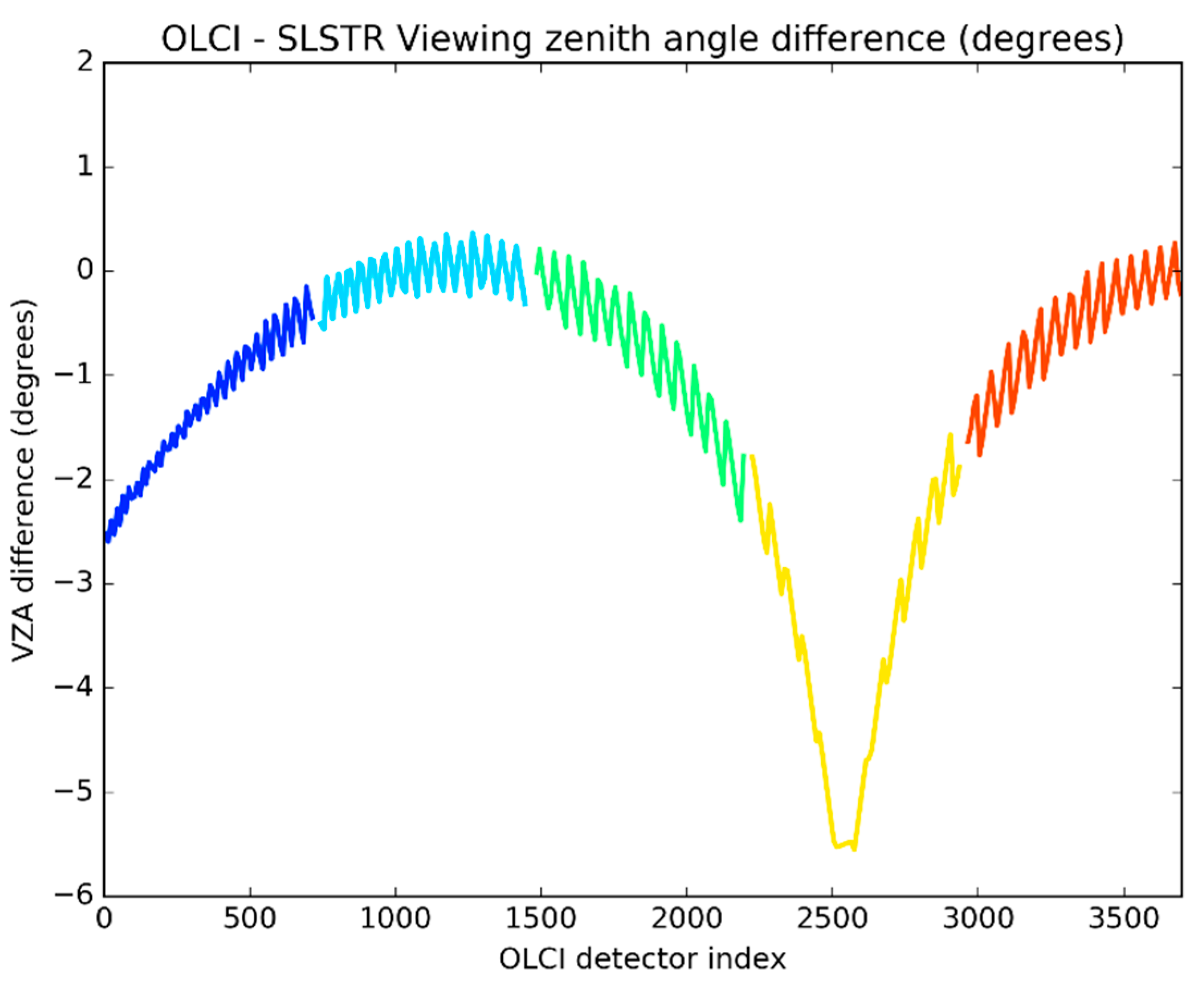
To answer this question, the best opportunity is found from the direct synergy with Sentinel-3 Sea and Land Surface Temperature Radiometer (SLSTR) on the Sentinel-3 platforms (see [1]). SLSTR and OLCI have been specifically designed to provide contemporaneous and co-located measurements of the same target scene. For our purpose, the SLSTR sensor notably provides nadir viewing acquisitions (in addition to oblique views) in three visible channels centered at 555 nm, 659 nm, and 865 nm that are spectrally close to equivalent OLCI channels. The conically scanning view geometry of SLSTR is markedly different that of OLCI. SLSTR continuously scans the ground using an array of detectors providing both a nadir scan view and a ‘forward’ inclined view at 53°. This configuration results in slightly different viewing angles across the OLCI FOV as reported in Figure 13, that directly impact the comparisons with OLCI, primarily through BRDF effects. Slight oscillations of the SLSTR viewing angle are also found across the OLCI FOV but do not degrade the analysis significantly as their effect translates into small-amplitude oscillations in the radiometric comparisons (see below in Figure 14).

What is most beneficial from this synergy is the relative comparisons of OLCI-A or OLCI-B with an independent reference measurement from SLSTR-A (being used in this special case although the conclusions are similar using SLSTR-B, not shown). Our focus is not to take SLSTR as an absolute radiometric reference but to compare the two OLCI sensors with respect to this reference, especially at the camera interfaces where the SLSTR scan is continuous, contrary to OLCI.

For the comparisons, the use of selected clouds targets again minimizes the impact of spectral shifts between OLCI and SLSTR (up to 6 nm differences, for instance leading to relatively stronger differences in ozone transmittance at 560 nm, resp. 555 nm) as well as of BRDF effects which can however be appreciated as a smooth modulation across the OLCI FOV without strong and abrupt changes, and (more importantly) without signal discontinuity along camera interfaces.

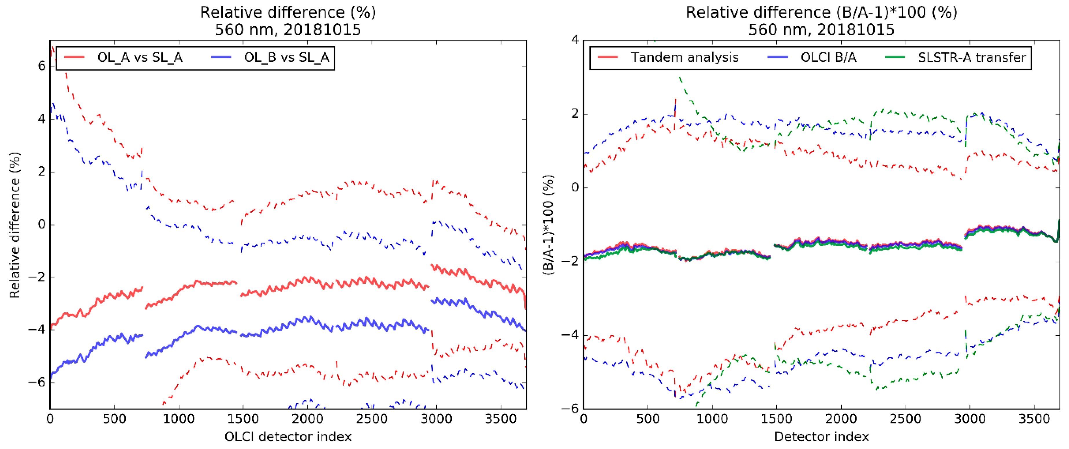
We have used all pre-reprocessing (i.e., not harmonized) data from 15 October 2018. Results are displayed in Figure 14 for Oa06 (560 nm) (supplement Figure S8 for the three bands but all of those provide similar results qualitatively). Raw differences of OLCI-A (respectively OLCI-B) to SLSTR-A are shown to the left. Comparisons to the tandem results are displayed to the right: results from the homogenized datasets comparison over selected clouds, ratios between OLCI-A and OLCI-B over the dataset collocated with SLSTR-A, and double-difference ratios between the differences with SLSTR (thus using SLSTR-A as a transfer sensor).

The drawbacks of the method (not same geometry nor exact wavelength of acquisition between OLCI and SLSTR) are surpassed by the benefits of the comparisons clearly showing that the two OLCI sensors compare very equally to SLSTR-A (apart from radiometric biases highlighted in the preceding sections) with similar discontinuities at camera interfaces. Especially between cameras 1 and 2 and between cameras 4 and 5, it is striking to see between 0.5 and 1.5% discontinuities between adjacent cameras, similarly for both OLCI sensors, which can only be due to a lack of camera equalization in the OLCI calibration, the discontinuities being slightly more pronounced for OLCI-B at camera 4/5 interface. The dispersion (dashed lines) increases with increasing viewing angles to the left and is minimal for the smallest viewing angle differences positioned around OLCI detectors 1200 and 3700.

This proves, at least for the three considered wavebands, that the two OLCI sensors behave remarkably similarly, even reproducing inter-camera discontinuities. These results could reasonably be generalized to the other bands, considering the spectral continuity of the tandem inter-calibration. Further proof on this matter can however be obtained from individual statistics of OLCI-A and OLCI-B camera interfaces over clouds.

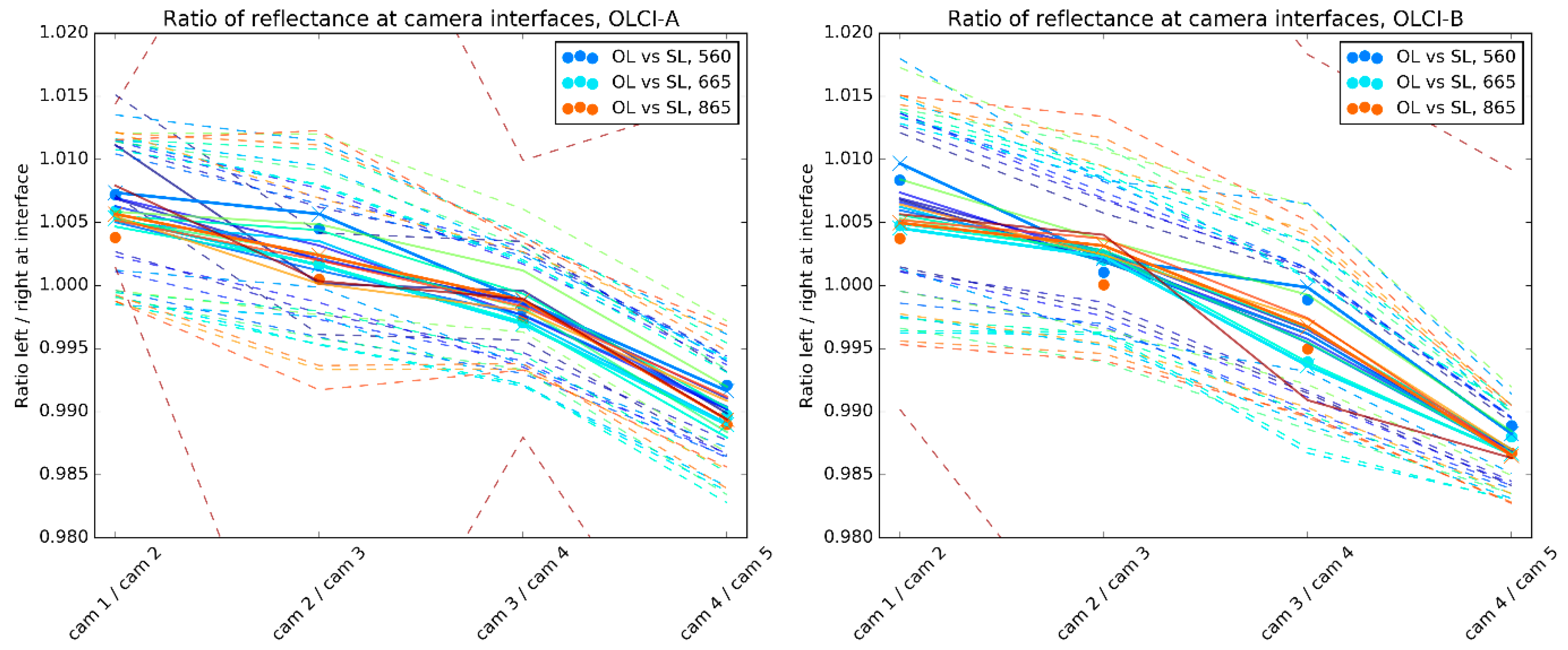
Indeed, a very simple algorithm is implemented (and processed independently over OLCI-A and OLCI-B L1B products) to scan clouds at each camera interface. Per row of L1B product (i.e., ACT line), a sample of 40 pixels (20 pixels for each camera) is taken at each camera interface provided that all pixels are tagged as cloudy (detected from the “bright” L1 flag). A threshold (value 0.0025) on the dispersion of the reflectance is applied to keep the most stable samples (mean reflectance below the threshold), it must be verified for each side of the interface individually (i.e., each camera). Over the selected samples, the ratio between mean reflectance from the left camera to the mean reflectance from the right camera is kept for a final statistical analysis. For each band and each interface, median and dispersion of the left/right ratio distributions are computed.

The obtained values are obtained for all bands and allow to quantify relative radiometric discontinuities between the cameras, as obtained from the colocation with SLSTR for only three wavebands (Figure 14 and Figure S8). For the comparison, the values corresponding to the discontinuities in Figure 14 are provided in coloured dots. Only the detectors closest to the interfaces are selected, no BRDF correction being deemed necessary for the purpose.

Figure 15 displays for OLCI-A (left) and OLCI-B (right) the medians and dispersions obtained for all bands from the cloud analysis in plain lines (dispersions in dashed lines) with colours ranging from deep blue (400 nm) to deep red (1020 nm). The ratios from the SLSTR collocation analysis are scattered in big dots with the colours associated to the three wavebands common to OLCI and SLSTR. These values were computed from tandem data from the same date (15 October 2018) as previously, very similar results can be obtained, individually for each sensor, from post-tandem data statistics (not shown).

Values are found the largest at interfaces between cameras 1 and 2 (about 0.5 %), even more between cameras 4 and 5 (about 1%, slightly more for OLCI-B) with consistency (yet noise) for all bands. The results from the SLSTR collocation analysis corroborates these findings. Considering all results, we conclude that OLCI-B camera 3 is the darkest.

It must be noted that these values are computed at camera interfaces, i.e., from measurements at the edges of the cameras which are suspected to be impacted by slight calibration residuals compared to the camera centres. There is no means to extrapolating these relationships to the whole cameras without changing the satellite attitude. The ideal approach to assess cross-detector calibration would be to perform yaw manoeuvres so that the cameras all viewed the same target along-track for a small period of time, ideally over homogeneous and/or bright targets. We strongly recommend this approach is included in any future Tandem flight with Sentinel-3C and Sentinel-3D.

However, we can base on these results to test an empirical flat-fielding approach for both sensors and quantify the consequences on the cross-calibration of OLCI-A and OLCI-B. From Figure 15 we can roughly estimate a mean alignment of the cameras from the mean figures obtained for each sensor individually and for each of the four camera interfaces. Relationships at 400 and 1020 nm are removed from the computation as we consider these as outliers, as well as for relationships at 560 nm at camera 3 (see below).

We make the hypothesis that the edge calibration residuals affect each camera symmetrically and identically so that the relationships hold for the complete cameras. We use camera 3 as the reference, the reason for this being its central position. We then propagate the mean ratios from camera 3 to each side of the FOV to compute relative alignment coefficients of all cameras relative to camera 3. We obtain the mean values reported below in

Table 2. Mean flat-fielding adjustment coefficients for OLCI-A and OLCI-B computed from the results of Figure 15.

	Cam 1	Cam 2	Cam 3	Cam 4	Cam 5
OLCI-A	0.992	0.997	1.000	0.998	0.988
OLCI-B	0.991	0.997	1.000	0.996	0.983

.

As we can see, these coefficients summarize the observation that all cameras are brighter than camera 3, that OLCI-A and OLCI-B behave similarly, and especially that cameras 5 are brighter of about 1% for OLCI-A and 1.5% for OLCI-B. Whereas these proportions are within the radiometric specifications of the OLCI mission, such differences translate into much larger differences (about a factor 10 proportionality) on BOA products, especially for water-leaving reflectance. Impact on these latter are quantified in more details in [5] where ACT flat-fielding is shown to be particularly required.

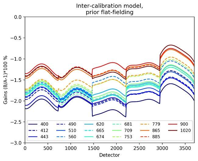
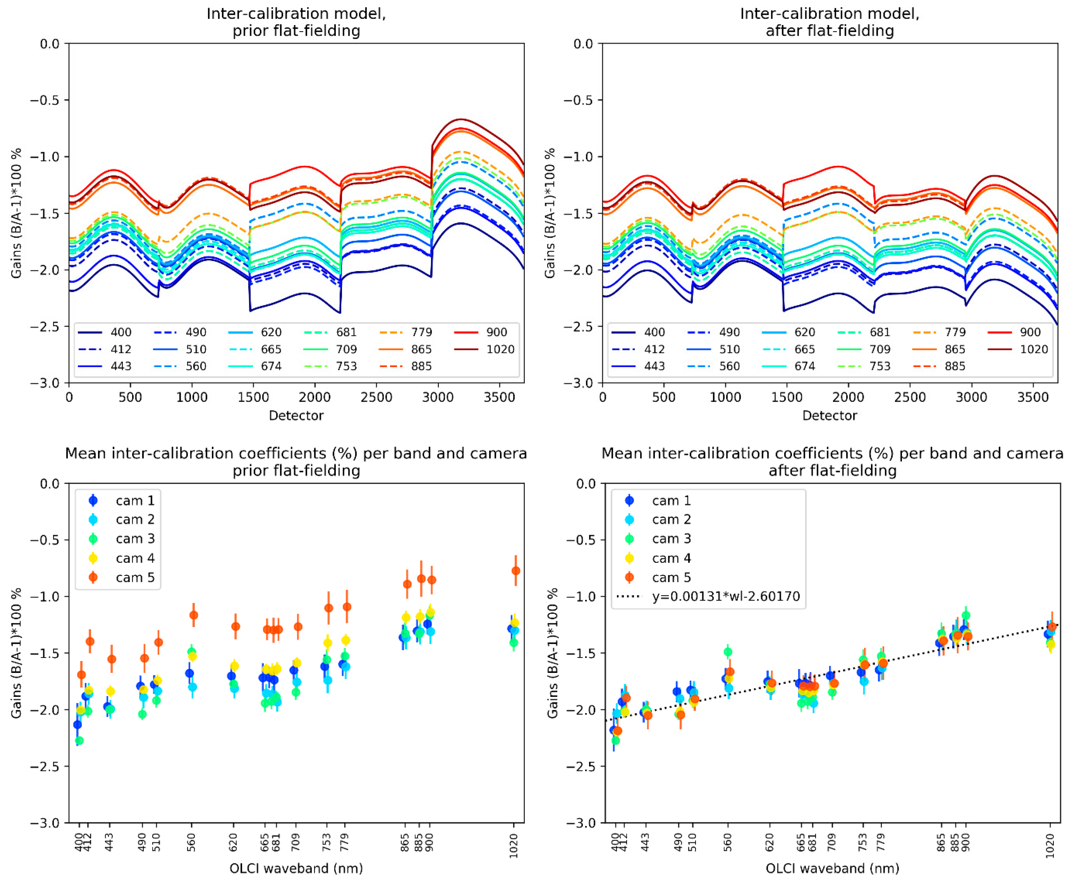
We quantify the impact on the inter-sensor calibration coefficients by applying, a posteriori, the flat-fielding coefficients to the corrected reflectance ratios OLCI-B/OLCI-A and directly compare the model in Figure 16 (top) prior to (left) and after (right) applying flat-fielding. In addition are displayed (bottom) mean inter-calibration coefficients computed per band and camera along with associated dispersions (i.e., standard deviations of all results per detector bins within each camera).

After applying flat-fielding, it is clear that the tandem inter-calibration results now appear much more aligned across the FOV thanks to the individual and independent flat-fielding of the two OLCI sensors. This even allows to consider performing a linear regression of the inter-calibration coefficients against the wavelength, independently of the camera, in the bottom right plot of Figure 16. This linear regression reads $g=0.001308 \lambda -2.60170$ with $\lambda$ the wavelength in nanometers.

Figure 16 highlights the relative exception of the intercalibration gain at 560 nm for camera 3. A possible explanation could lie in the larger differences in spectral responses for this camera (see Figure 4). As a result, the hypothesis of similar ozone transmissions for OLCI-A and OLCI-B may not hold for this camera.

Differences between the linear regression model and the inter-calibration coefficients give an insight on the relevance of a pragmatic flat-fielding and inter-calibration approach. Minimum and maximum departures from the model are respectively −0.23% and 0.38% difference between OLCI-A and OLCI-B, the dispersion of the differences being 0.11%.

Applying the values of Table 2, individually on each OLCI, and then the linear regression above provides any L1B product user with the ability to align the radiometry of the sensors. We recommend these pragmatic corrections until reprocessed data and operational products are more properly aligned (e.g., would flat-fielding be better assessed from yaw manoeuvres or any other technique or methodology).

For future Sentinel-3C and Sentinel-3D OLCI sensors, the approach will need to be re-evaluated depending on the relative performances of each sensor at that time.

7. Conclusions

Cross-sensor comparisons are usually employed for radiometric validation purposes (e.g., [22,23,24]. In this particular case, the two OLCI payloads are twin sensors which share the same characteristics but have slight differences in their manufacturing corresponding to limitations in industrial reproductibility. The tandem phase is a unique opportunity to intercompare and intercalibrate the sensors for mission continuity requirements. This provides ideal conditions (two similar payloads observe the same targets nearly simultaneously), allowing to bypass stronger spectral, radiometric, and geometric differences usually faced by cross-sensor comparisons, as well as providing huge statistics out-performing comparisons between different missions.

We have presented and validated a homogenisation and harmonisation methodology of OLCI-A and OLCI-B L1B TOA radiances. Homogenisation consists of reprojecting measurements on the same comparison grid and adjusting the sensors radiometry for slight spectral shifts. Harmonisation consists of aligning the two sensors radiometry considering the differences in the homogenised radiometries. One finding for the methodology is the unexpected quality of the comparisons obtained from cloud targets: cloud motion and parallax effects are largely compensated by the huge statistics, as well as by the strength and the whiteness of the signal over these targets. Indeed, cloud observations, which are favorized against the other targets, do not require sophisticated spectral adjustment models, unlike water and land targets (including deserts). Comparisons over desert areas provide a second-best solution with faster convergence (less than 10 min of tandem data are necessary to provide a result) and smaller dispersion due to the homogeneity and signal strength over these targets.

The most important finding is the evidence of a 1% to 2% bias between the two OLCI payloads. There is no clear evidence of the reason for this bias as both sensors are nominally and successfully calibrated in-flight, although we suspect that on-board diffuser pre-flight characterization can be the culprit. The harmonisation is validated in this paper using data products obtained from a dedicated custom reprocessing. Intercalibration of OLCI-A and OLCI-B is shown to provide a performance better than 0.5%, which is an excellent performance. Clear benefits at L2 are assessed in a companion paper [5], further providing confidence in such harmonisation.

Discussing the need of a reference for the OLCI “system of systems”, strong evidence of camera discontinuities is found from synergy with SLSTR as well as from analyses of camera interfaces over clouds. Despite the two OLCI sensors behaving similarly across the FOV, both exhibit undesired camera radiometric biases, especially between cameras 4 and 5. Applying a pragmatic flat-fielding procedure, individually on both sensors, considerably homogenises the inter-calibration coefficients between cameras. It further allows to provide the L1B product user with a simple, yet accurate, relationship between the A/B inter-calibration coefficients and the wavelength of acquisition.

As a final conclusion, we strongly support the use of tandem phasing for future optical sensors (e.g., next OLCI-C and -D, Sentinel-2, FLEX/OLCI), which have proven to be extremely useful as highlighted in this paper. Benefits for other Sentinel-3 payloads have been addressed in the Sentinel-3 Tandem for Climate (S3TC) study. Tandem conditions shall be in line with the ones met here for OLCI-A and -B which prove to be efficient. It is of prior importance to have a good knowledge on the spectral and radiometric characterisation of the compared sensors individually, it therefore requires prior in-flight verification of the instrument’s calibration and characterisation as well as traceability of the sensor’s calibration. A separation of 30 s between satellites is efficient for the comparisons (although a shorter separation might decrease the dispersion, convergence would be even faster) but a longer delay may nullify the use of clouds for the comparisons (longer separations would result in the almost exclusive use of desert areas which are the most stable targets). Four months of tandem have been used to validate the temporal consistency of daily robust statistics for the intercalibration of Sentinel-3A and Sentinel-3B OLCI (which is achieved using much less data from an engineering perspective).

To maintain the climate record, it is highly recommended that the future Sentinel-3C and Sentinel-3D satellites perform tandem flights when injected into the Sentinel-3 time series. As final recommendations for future OLCI sensors, we strongly recommend a better knowledge of the diffusers pre-flight BRDF characterization, and/or performing yaw manoeuvers for cross-detector calibration across the complete FOV. Until such a manoeuvre is performed, we can only rely on empirical methods such as presented in this paper to perform the equalization of OLCI cameras prior to the radiometric alignment of OLCI sensors.