Periodic Relations between Terrestrial Vegetation and Climate Factors across the Globe

Abstract

In this paper, cross-spectrum analysis was used to verify the agreement of periodicity between the global LAI (leaf area index) and climate factors. The results demonstrated that the LAI of deciduous forests and permanent wetlands have high agreement with temperature, rainfall and radiation over annual cycles. A low agreement between the LAI and seasonal climate variables was observed for some of the temperate and tropical vegetation types including shrublands and evergreen broadleaf forests, possibly due to the diversity of vegetation and human activities. Across all vegetation types, the LAI demonstrated a large time lag following variation in radiation (>1 month), whereas relatively short lag periods were observed between the LAI and annual temperature (around 2 weeks)/rainfall patterns (less than 10 days), suggesting that the impact of radiation on global vegetation growth is relatively slow, which is in accord with the results of previous studies. This work can provide a benchmark of the phenological drivers in global vegetation, from the perspective of periodicity, as well as helping to parameterize and refine the DGVMs (Dynamic Global Vegetation Models) for different vegetation types.

1. Introduction

Knowledge about the response of vegetation to climate change is crucial for understanding ecosystem dynamics [1]. Rainfall, solar radiation and temperature are the main climate constraints that determine the spatial distribution of ecosystems and vegetation growth [2,3,4]. In previous studies, the impacts of these climate factors on phenological cycles of global vegetation in different regions have been widely investigated by using both ground-based methods and remote sensing technology [5,6,7,8,9,10,11]. However, the agreement of seasonal variation and the time lag effect of climate factors on terrestrial vegetation remain unclear at the global scale, increasing uncertainty in Dynamic Global Vegetation Models (DGVMs).

Global vegetation shows different properties of phenological cycles across vegetation types, which is mainly caused by the local climate features. For example, most temperate vegetation tends to have an annual cycle of growth [12], whereas vegetation in the tropics (most are evergreen forests), especially in tropical rainforests, has no evidence of annual growth cycles at large scales [13]. Meanwhile, vegetation with more than one phenological cycle per year is mainly distributed in the regions where there are two rainy seasons per year [14], as well as in some other regions where both winter temperatures and summer water availability constrain the growth of vegetation [15]. Over large scales, there are two main approaches for detecting the phenological cycle of vegetation using remotely sensed data. The first is to identify the number of peaks in the growth curve extracted from time series data (like different vegetation indices) for each year as the number of cycles [13], and the second approach in identifying phenological cycles utilizes the spectral analysis method (e.g., Fourier analysis) to extract the traits of the different cycles [12]. The vegetation parameters, such as leaf area index (LAI) and fractional vegetation coverage (FVC), are key agronomic and ecological parameters, which are of great importance to the study of hydrology, ecology and global change [16,17].

Previously, most large scale climate-vegetation studies adopted simultaneous climate and vegetation indicators and did not consider the time lag effect of climate variables on vegetation [18]. The time lag effect can be defined as the impact of climate factors, i.e., historical rainfall and temperature regimes, on current vegetation dynamics and are also described in reference to climate legacies [19]. The legacies of short-interval climate events are dependent on three main indicators: (1) the magnitude of the historical climate event or regime, (2) the time elapsed since its occurrence and (3) the sensitivity of the system to the event [20,21,22,23]. On the whole, a large climate event will result in a prolonged change in vegetation growth, while small climate fluctuations tend to have short influences on a small fraction of the vegetation. For example, an increase in the carbon dioxide efflux from the soil can lead to a rapid detectable improvement of photosynthesis with a short time lag of several hours to days (d) in different vegetation types [24]. By contrast, extreme drought can quickly reduce the growth of native plants; yet this negative growth impact can last for several years until the plants are completely recovered [25,26]. In addition to the impacts of short-term events on vegetation growth, some studies have also investigated the positive and negative time lag effects of climate factors on vegetation growth over longer time periods, by correlating current period vegetation conditions and current/previous climate factors. However, in these cases, the short temporal resolution (such as monthly) of remotely sensed data often limited the accuracy of measuring the time lag effect [27,28,29,30,31].

Herein, we conducted cross-spectrum analysis of a long time series of Global Land Surface Satellite (GLASS) LAI data and European Union Water and Global Change-Forcing-Data-ERA-Interim (WFDEI) climate datasets (1981–2014) to (1) examine the agreement of phenology between vegetation and three climate variables (i.e., radiation, temperature and rainfall) in different terrestrial vegetation types and (2) study the time lag effect for climate variables on vegetation.

2. Materials and Methods

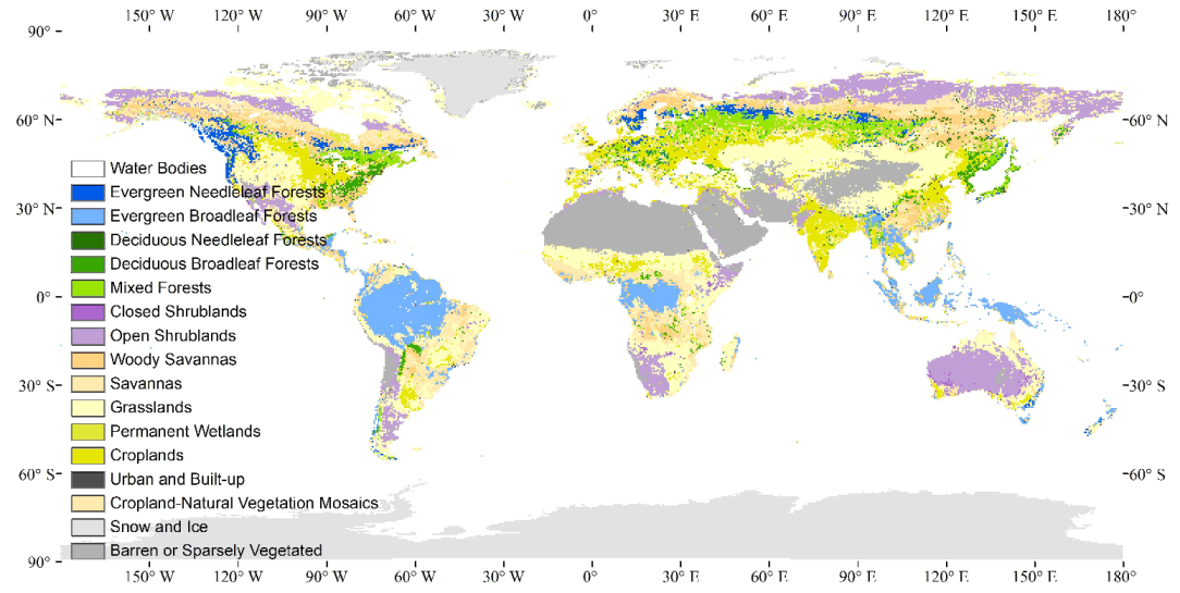
2.1. Global Vegetation Classification

In this study, we used the International Geosphere-Biosphere Programme (IGBP) classification data to define ecosystem surfaces into 17 general land cover types, including 12 natural vegetation classes, three developed land classes and two water classes [32]. We selected 13 vegetation types for analysis, excluding water bodies, urban and built-up areas, and snow and ice areas, along with barren or sparsely vegetated areas (Figure 1). The Terra and Aqua combined Moderate Resolution Imaging Spectroradiometer (MODIS) Land Cover Climate Modeling Grid (CMG; MCD12C1) Version 6 data product provides a spatially aggregated and re-projected version of the tiled MCD12Q1 Version 6 data product. This dataset includes IGBP classifications and two additional classification schemes at a 0.05° (~5600 m) spatial resolution [33].

2.2. LAI Data

The GLASS LAI data from 1981 to 2014 were acquired from the Chinese National Earth System Science Data Sharing Infrastructure website (http://www.geodata.cn/thematicView/GLASS.html) [34,35]. The spatial and temporal resolutions for the LAI data were 0.05° and 8 d, respectively. In the production process for GLASS LAI, the cloud-contaminated data were identified by snow and cloud mask data and then removed using spatiotemporal filtering algorithms. The missing data were filled in using an optimum interpolation algorithm to obtain continuous and smooth surface reflectance values [36]. This process reduces the influence of clouds to the maximum extent, especially in the tropics.

2.3. Climate Data

We used daily rainfall, mean air temperature and shortwave radiation (referred to as radiation through the text) datasets from 1981 to 2014 to analyze the agreement between vegetation growth and climate variables, and the time lag effect of climate factors on vegetation growth by resampling remotely sensed data into a spatial resolution of 0.5° using the nearest interpolation method. These three climate variables have been widely appointed as the predominant influencing factors for the phenology of terrestrial vegetation [37,38,39]. Climate data were generated from the European Union Water and Global Change project (http://www.eu-watch.org), which provides a gridded Water and Global Change Forcing Data ERA-Interim (WFDEI) data product with a spatial resolution of 0.5° and has relative data extending back to 1979 [40,41].

2.4. Cross-Spectrum Analysis

Spectrum analysis is used to extract the characteristics of periodicity in a spectrum (or time series data) [42,43]. Spectrum analysis can be classified into single-spectrum analysis and cross-spectrum analysis based on the quantity of research objectives. Single-spectrum analysis stresses the characteristics of periodicity in one spectrum, while cross-spectrum analysis focuses more on the relationship between variation in two spectra (or time series data) in the frequency domain. If we set functions x1(t) and x2(t) to represent two kinds of time series data, the covariance of them can be written as below:

$${\displaystyle \underset{-\infty }{\overset{\infty }{\int }}{\mathrm{x}}_1(\mathrm{t})}{\mathrm{x}}_2(\mathrm{t})\mathrm{dt}=\frac{1}{2\mathsf{\pi }}{\displaystyle {\int }_{-\infty }^{\infty }{\mathrm{F}}_2(\mathsf{\omega }){\mathrm{F}}_1(-\mathsf{\omega })\mathrm{d}\mathsf{\omega }}$$

(1)

where F means Fourier transform and ω is the circular frequency. The covariance shows the cross energy of the two time series data. The cross spectrum of them can be defined as:

$$\begin{array}{ll}{\mathrm{S}}_{12}(\mathsf{\omega })& ={\mathrm{F}}_2(\mathsf{\omega }){\mathrm{F}}_1{}^{*}(\mathsf{\omega })\\ & ={\mathrm{P}}_{12}(\mathsf{\omega })-\mathrm{i}{\mathrm{Q}}_{12}(\mathsf{\omega })\end{array}$$

(2)

The real part spectrum is called the co-spectrum, and the imaginary part spectrum is the orthogonal spectrum. It can also be written in terms of amplitudes and phases as:

$${\mathrm{S}}_{12}(\mathsf{\omega })={\mathrm{A}}_{12}(\mathsf{\omega }){\mathrm{e}}^{\mathrm{i}{\mathsf{\theta }}_{12}(\mathsf{\omega })}={\mathrm{A}}_{12}(\mathsf{\omega })\times {\mathrm{e}}^{\mathrm{i}\times \mathrm{t}{\mathrm{g}}^{-1}(\frac{{\mathrm{Q}}_{12}(\mathsf{\omega })}{{\mathrm{P}}_{12}(\mathsf{\omega })})}$$

(3)

where A₁₂ and θ represent the amplitude and phase of the cross spectrum, respectively. Then, we define the condense spectrum as:

$${\mathrm{R}}_{{}^{12}}^2(\mathsf{\omega })=\frac{{\mathrm{P}}_{12}^2(\mathsf{\omega })+{\mathrm{Q}}_{12}^2(\mathsf{\omega })}{{\mathrm{P}}_{11}(\mathsf{\omega }){\mathrm{P}}_{22}(\mathsf{\omega })}$$

(4)

which shows the relationship between two time series data at a specific frequency (ω). For the locations where there is an annual cycle in both the phenology time series and a driver, the coherency (i.e., the degree of correlation at specific frequencies; range: 0.0–1.0) was calculated. Meanwhile, we used the time lag spectrum (Equation (5)) to estimate the corresponding time lag (from the value of phase difference) with the same frequency (T represents the cycle) [44,45].

$$\mathrm{L}(\mathsf{\omega })=\frac{{\mathsf{\theta }}_{12}(\mathsf{\omega })\times \mathrm{T}}{2\mathsf{\pi }}$$

(5)

This method has been commonly used in disciplines such as medicine, economics and physics [46,47,48]. Here, we apply cross-spectrum analysis to the LAI of global vegetation and driven climate data at a long temporal scale, which enables us to estimate the agreement between climate variables and the growth cycle. Furthermore, we classify the result of common cycles into three groups: (1) an annual common cycle of vegetation growth with climate data; (2) other common cycles, i.e., where multiple common cycles were detected per year; or (3) no common cycle, i.e., where there is no significant relationship between vegetation growth and climate variables. Here, the common cycle was defined as the cycle with the highest coherency between the time series data of the LAI and climate factors by cross-spectrum analysis (P < 0.05). This approach was mainly realized by inserted functions in MATLAB.

2.5. Categorizing Phase

The phase or time lag relationships were grouped into four categories, “in phase”, “antiphase”, “leads” and “lags”, which were detailed in previous research [49]. The four categories can be demonstrated in one full circle (with phenology of LAI located in the position of 0°) and the specific standards for the classification are as follows:

• The driver (climate variable) and the phenology (LAI) are “in phase”: the phase value is statistically indistinguishable (given the phase error) from 0° ± 30° (or 0.0 ± 1.0 months);
• The driver “leads” the phenology: a positive phase that is between + 30° (or +1.0 month) and +150° (or +5.0 months);
• The driver and phenology are “in antiphase”: a phase value that is statistically indistinguishable from 180° ± 30° (or 6.0 ± 1.0 months);
• The driver “lags” the phenology: a negative phase between −30° (or −1.0 months) and −150° (or −5.0 months).

This method was proved to be a robust means of the statistical classification of phenology-driver (climate variable) phase differences, avoiding manual thresholds that were dependent on the dataset [50].

3. Results

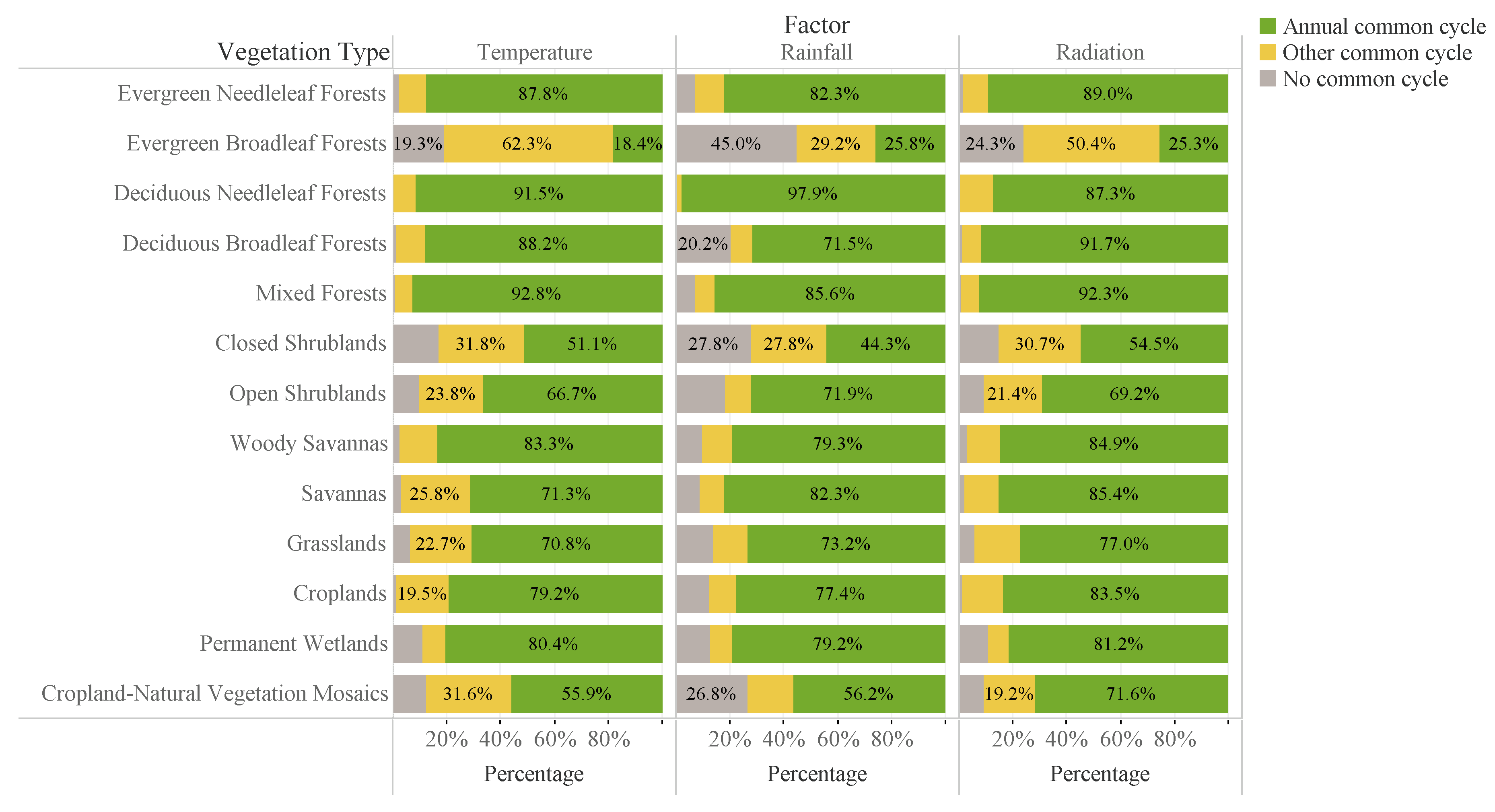
3.1. Common Cycles of LAI and Climate Data

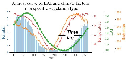
Of the 13 vegetation categories studied here, the majority of the vegetation types demonstrated an annual common cycle for temperate vegetation growth with climate factors (>71.5% annual common cycle for temperate forests; Figure 2). However, the proportion of annual common cycle in evergreen broadleaf forest was reduced, with temperature, rainfall and radiation accounting for only 18.4%, 25.8% and 25.3%, respectively, of the variation. However, in other forests (mainly distributed in subtropical area of South America and Africa, and northern high latitudes mainly between 30°N and 60°N), permanent wetlands and croplands, the proportion of annual common cycle was much higher. For example, in deciduous needleleaf forests, the proportions were 91.5%, 97.9% and 87.3% with temperature, rainfall and radiation, respectively, indicating high periodic agreement between vegetation and climate factors on an annual basis. Although still dominated by an annual common cycle, shrublands, savannas and grasslands demonstrated a reduced agreement between the periodicity in the LAI and climate variables.

Meanwhile, the characteristics of the common cycle of the LAI with different climate factors appears to be diverse. If we compare rainfall with temperature based on the proportion of annual common cycle with the LAI, we can see that in evergreen broadleaf forests, the value of temperature (25.8%) is larger than that of rainfall (18.4%). This comparison is similar in deciduous needleleaf forest. However, in evergreen broadleaf forest and some other vegetation types like open shrublands, savannas and grasslands, the proportion of annual common cycle with the LAI is larger for rainfall than for temperature. In addition, radiation tends to have a large proportion of annual common cycle with the LAI in most of the vegetation types of forests.

3.2. Time Lag

As we have 13 vegetation types and three climate variables, we can pair them into 39 “vegetation-drivers” categories for comparison (

Table 1. The time lag of LAI and the phase categories with three climate variables on an annual basis. The radar charts represent the distribution of the time lag with the temperature, rainfall and radiation, respectively; the annual scale was mapped over 360°. Each line in the circle marks the value of time lag for each pixel, while a darker color reveals more pixels assembling in the region of the corresponding time lag. The black line refers to the average value of the time lag, and the green line represents the position of the average value ± std in each case. The area of the bar in each cell shows the percentage of each phase category. The unit of the mean and std is days (d).

Vegetation Types	Temperature	Rainfall	Radiation
Evergreen Needleleaf Forests
Evergreen Broadleaf Forests
Deciduous Needleleaf Forests
Deciduous Broadleaf Forests
Mixed Forests
Closed Shrublands
Open Shrublands
Woody Savannas
Savannas
Grasslands
Permanent Wetlands
Croplands
Cropland-Natural Vegetation Mosaics

). From the result, we can see that the majority of categories (37 out of 39) demonstrated a positive mean value for the time lag of the LAI with a seasonal change of the climate variables over an annual cycle. In addition, radiation has the largest time lag with the LAI among the three climate factors, with an average time lag of 39.6 d for 13 vegetation types, compared to 13.4 d for temperature and 9.9 d for rainfall, respectively.

Temperate and boreal forests, such as deciduous needleleaf forests and deciduous broadleaf forests, were dominated by an annual common cycle (all over 70% with the climate variables, Figure 2). These forests also demonstrated short time lag periods following variation in temperature and rainfall with a high degree of confidence in these values (e.g., in deciduous broadleaf forests, temperature and rainfall were “in phase” with > 83% correlation of the data to the phase pattern, equating to a time lag of 8.1 ± 20.7 d for temperature and 5.8 ± 23.2 d for rainfall) but responded slowly to radiation (e.g., radiation “leads” changes in the LAI by 40.5 ± 44.7 d for deciduous broadleaf forest). Meanwhile, the percentage of the “in phase” pattern for temperature and rainfall in deciduous broadleaf forests accounts for 86.4% and 83.5%, respectively. In permanent wetlands, there is a widespread “in phase” relationship of the LAI with both temperature (93.5%) and rainfall (95.2%), while the corresponding average value of time lag is 13.2 ± 14.8 d (with temperature) and 2.0 ± 11.6 d (with rainfall), showing a greater influence of temperature and rainfall on vegetation in this region. Therefore, in temperate/boreal forests and permanent wetlands, not only do the different forest types have a very consistent growth rhythm with temperature and rainfall but these two factors also have a direct and quick impact on vegetation growth within a short time lag.

In evergreen broadleaf forests (Table 1), which can be attributed to be in the same region as tropical rainforest, the time lag of the LAI with all three climate factors is much larger than those in temperate and boreal forests and all three variables are classified as “leads”. Among them, radiation has the largest average value of time lag (45.8 ± 113.2 d), followed by temperature (36.7 ± 41.5 d) and rainfall (27.6 ± 62.0 d). The standard deviation (std) is over 40 d for all three variables, implying that the spatial complexity of the interaction between the vegetation and climate variables in this area is large. Closed shrublands also follow a similar pattern to tropical vegetation, with all climate variables leading the LAI change (> 55%), and the std was very large. By contrast, the savanna vegetation category followed a similar trend to temperate forests with a strong “in phase” relationship of the LAI with rainfall and temperature (> 78%), with a short time lag for rainfall (4.5 ± 26.5 d for woody savannas and 11.2 ± 29.7 d for savannas), while the average time lag with temperature is larger (11.1 ± 20.1 d for woody savannas and 21.0 ± 37.0 for savannas). However, in both savanna vegetation categories, the std was again large, indicating complexity in these systems.

Across all vegetation, with the exception of croplands and evergreen broadleaf forests, there is a widespread “leads” relationship between radiation and the LAI (with a percentage for “leads” in excess of 66%; Table 1). The impact of radiation has a much larger time lag in its impact on different vegetation, averaging a time lag of 39.6 ± 53.5 d, inferring that radiation has little influence on most vegetation on a short-term basis. Croplands show a very discrete and highly variable distribution of time lag with temperature (7.1 ± 50.4 d), rainfall (17.9 ± 34.6 d) and radiation (23.7 ± 73.6 d; Table 1). The percentage of the “in phase” pattern of time lag with temperature, rainfall and radiation only accounts for 69.7%, 69.7% and 39.4%, respectively, which is relatively low in comparison with those of the other vegetation types (Table 1).

4. Discussion

In temperate forests (mainly consisting of deciduous broadleaf forests and deciduous needleleaf forests) and wetlands, a high percentage of annual common cycle and a short time lag between the LAI and temperature/rainfall was observed in the cross-spectrum analysis, which indicates that vegetation in these regions has the greatest agreement between the LAI and the two climate variables, compared with other vegetation types across the globe. However, in tropical forests (mainly covered by evergreen broadleaf forests), vegetation can obtain enough heat throughout the year. In this case, the function of rainfall is expanded, and water availability often become the limiting factor for vegetation growth [51,52,53], which was proved by the higher percentage of annual common cycle, as well as the smaller time lag between the LAI and rainfall in this region. However, the cyclical relationships between LAI and climate factors also demonstrated a high spatial variation in evergreen broadleaf forests, as the low percentage of annual common cycle and high standard deviation of the time lag indicate. The explanation for this phenomenon is that in the region of high latitude in the Northern Hemisphere, there is a strong seasonal variation in solar radiation, which drives strong seasonal variation in temperature, rainfall and the LAI. The vegetation growth in this area has very distinct phenology, which is mainly influenced by local climate factors through the year [54,55]. By contrast, climate factors vary less in one year in the tropics, so the vegetation growth there is more restricted to the local environment, and the uniform rule for the influence of meteorological data on vegetation is not easy to detect [56,57].

In addition to tropical forests, vegetation impacted by human intervention, such as croplands, tended to have low correlation with the annual common cycle and climate variables. Within this vegetation classification, most vegetation was planted by humans to meet different agricultural demands rather than natural growth, replacing the original vegetation with annual crops or pastures, and is under the influence of the farm management cycles. Therefore, crops with two or three harvests each year may induce a low percentage in the annual common cycle [58,59,60]; in addition, the building of greenhouses and irrigation regimes decreases the impact of temperature and rainfall on crop species. For cropland–natural vegetation mosaics, the correlation to an annual common cycle is also reduced, possibly due to mixed vegetation within one pixel. Meanwhile, in savannas (including savannas and woody savannas) and grasslands, rainfall has also been shown to be the predominant driver for vegetation phenology, as illustrated by the high percentage of annual common cycle and short time lag between the LAI and rainfall, with temperature as a concomitant variable [61,62], due to the extreme difference in the quantity of rainfall between periods of rainy season and dry season [63,64].

Our spectrum analysis also indicated a long time lag in all vegetation categories, with the exception of cropland, between the LAI and radiation (having a high percentage of data within the “leads” category) compared with temperature and rainfall, despite there being a strong correlation of the LAI to radiation for most vegetation types on an annual basis. Wu et al. [18] and Notaro et al. [65] also demonstrated this phenomenon, reporting a similar one month time lag in most of the middle and high latitudes of the Northern Hemisphere, and, as in our study, the time lag varied significantly in other vegetation regions. The reason for this phenomenon is that terrestrial vegetation reacts to variation in radiation by changing its strategies for absorbing photosynthetically active radiation (PAR) gradually, therefore increasing light use efficiency, creating the lag in the response [66]. Previous studies also show that air temperature is highly correlated with a roughly one-month-lag insolation in different parts of the world, and they used this relationship to create equations for the simulation of regional temperature with local insolation as an input [67,68]. Meanwhile, for the ocean, the corresponding time lag will be two to three months, due to the specific heat capacity of water with similar energy inputs [69]. Therefore, solar radiation not only has a direct influence on vegetation but also has indirect impact on vegetation through temperature and rainfall in some specific areas. Based on global meteorological data, researchers have also demonstrated that there is a lag in the temperature response after solar radiation changes, which could also account for the long time lag response of vegetation to radiation but the relatively rapid response to temperature, widely across the world [70].

The spectrum analysis helps us to better understand the impact of climate on annual vegetation growth cycles and the time lag effect. This method has not been widely used globally but proved to be valid and effective in this study on phenology and the interactions between climate and terrestrial vegetation, as long as the relevant long time series of vegetation and climate data are available. However, it must be emphasized that the scale effect on periodic features of vegetation cannot be ignored. Namely, when using remotely sensed imagery from space-borne sensors, investigators are limited to specific scales of observation [71,72]. For example, in the tropics, where there is high spatial variability in both vegetation and microclimate, the spectral information of evergreen and deciduous forests might be both captured in the same pixel of remotely sensed data, which induces the uncertainty of phenological analysis. Tree ring analysis using dendrometer measurements indicates that the different vegetation types can have a large variation in growth cycle categories with quasi-annual cycles [73], annual cycles [74], two growth cycles per year [75] or even long-term growth categories being reported in the tropics [76]. This is because species with different growth strategies respond differently to climate events [77] under different local microclimates [78]. In addition, coupling different remotely sensed data by upscaling and resampling data from a smaller spatial resolution to higher spatial resolution may also create more uncertainty and inaccuracy. Therefore, future work might focus on the periodic features of vegetation and their relationship with climate variables over different scales.

5. Conclusions

In this paper, cross-spectrum analysis was used to extract the common cycle and time lag between the LAI of different global vegetation types and daily climate variables, including temperature, rainfall and radiation. Overall, there is a high percentage of annual common cycle, accompanied with a short time lag in the vegetation response to rainfall and temperature on an annual basis for most pairs of vegetation-drivers, with the exception of evergreen broadleaf forests, croplands and closed shrublands. Specifically, there is a very distinct periodic agreement between vegetation growth and all three selected climate factors for temperate, boreal forests and permanent wetlands, where vegetation responded to variation of the temperature and rainfall rapidly. Rainfall may trigger the phenological events of vegetation in savannas and woody savannas predominantly, compared with temperature, as indicated by the relatively high percentage of annual common cycle and smaller time lag between the LAI and rainfall in these regions. The human management of croplands and cropland mosaics has a large impact on the periodic relations between the LAI and climate factors, indicated by the low percentage of periodic agreement and large, highly variable time lag. Although the LAI and radiation have a good agreement on an annual basis in most vegetation types, cross-spectrum analysis identified a large time lag in the vegetation response. Our study provides a useful tool for identifying and parameterizing the potential periodic elements in future DGVMs by identifying the key characteristics and drivers of global vegetation phenology patterns.

References

1. Chen, T.; de Jeu, R.A.M.; Liu, Y.Y.; van der Werf, G.R.; Dolman, A.J. Using satellite based soil moisture to quantify the water driven variability in NDVI: A case study over mainland Australia. Remote Sens. Environ. 2014, 140, 330–338. [Google Scholar] [CrossRef]
2. Churkina, G.; Running, S.W. Contrasting climatic controls on the estimated productivity of global terrestrial biomes. Ecosystems 1998, 1, 206–215. [Google Scholar] [CrossRef]
3. Nemani, R.R.; Keeling, C.D.; Hashimoto, H.; Jolly, W.M.; Piper, S.C.; Tucker, C.J.; Myneni, R.B.; Running, S.W. Climate-driven increases in global terrestrial net primary production from 1982 to 1999. Science 2003, 300, 1560–1563. [Google Scholar] [CrossRef] [PubMed] [Green Version]
4. Stephenson, N.L. Climatic control of vegetation distribution: The role of the water balance. Am. Nat. 1990, 135, 649–670. [Google Scholar] [CrossRef]
5. Friedman, J.M.; Roelle, J.E.; Cade, B.S. Genetic and environmental influences on leaf phenology and cold hardiness of native and introduced riparian trees. Int. J. Biometeorol. 2011, 55, 775–787. [Google Scholar] [CrossRef] [Green Version]
6. Laskin, D.N.; McDermid, G.J. Evaluating the level of agreement between human and time-lapse camera observations of understory plant phenology at multiple scales. Ecol. Inform. 2016, 33, 1–9. [Google Scholar] [CrossRef]
7. Liang, B.; Liu, S.; Qu, Y.; Qu, Y. Estimating fractional vegetation cover using the hand-held laser range finder: Method and validation. Remote Sens. Lett. 2015, 6, 20–28. [Google Scholar] [CrossRef]
8. Liang, B.; Liu, S. Measurement of vegetation parameters and error analysis based on Monte Carlo method. J. Geogr. Sci. 2018, 28, 819–832. [Google Scholar] [CrossRef]
9. Liang, B.; Dahlsjö, C.A.; Maguire-Rajpaul, V.; Malhi, Y.; Liu, S. Modelling error evaluation of ground observed vegetation parameters. IEEE Trans. Instrum. Meas. 2019. [Google Scholar] [CrossRef]
10. Ma, M.; Veroustraete, F. Reconstructing pathfinder AVHRR land NDVI time-series data for the Northwest of China. Adv. Space Res. 2006, 37, 835–840. [Google Scholar] [CrossRef]
11. Morton, D.C.; DeFries, R.S.; Shimabukuro, Y.E.; Anderson, L.O.; Arai, E.; del Bon Espirito-Santo, F.; Freitas, R.; Morisette, J. Cropland expansion changes deforestation dynamics in the southern Brazilian Amazon. Proc. Natl. Acad. Sci. USA 2006, 103, 14637–14641. [Google Scholar] [CrossRef] [PubMed] [Green Version]
12. Menenti, M.; Azzali, S.; Verhoef, W.; Van Swol, R. Mapping agroecological zones and time lag in vegetation growth by means of Fourier analysis of time series of NDVI images. Adv. Space Res. 1993, 13, 233–237. [Google Scholar] [CrossRef]
13. Verger, A.; Filella, I.; Baret, F.; Peñuelas, J. Vegetation baseline phenology from kilometric global LAI satellite products. Remote Sens. Environ. 2016, 178, 1–14. [Google Scholar] [CrossRef] [Green Version]
14. Vrieling, A.; De Leeuw, J.; Said, M.Y. Length of growing period over Africa: Variability and trends from 30 years of NDVI time series. Remote Sens. 2013, 5, 982–1000. [Google Scholar] [CrossRef] [Green Version]
15. Julien, Y.; Sobrino, J. Global land surface phenology trends from GIMMS database. Int. J. Remote Sens. 2009, 30, 3495–3513. [Google Scholar] [CrossRef] [Green Version]
16. Nackaerts, K.; Coppin, P.; Muys, B.; Hermy, M. Sampling methodology for LAI measurements with LAI-2000 in small forest stands. Agric. For. Meteorol. 2000, 101, 247–250. [Google Scholar] [CrossRef]
17. Running, S.W.; Thornton, P.E.; Nemani, R.; Glassy, J.M. Global terrestrial gross and net primary productivity from the Earth Observing System. In Methods in Ecosystem Science; Springer: Berlin/Heidelberg, Germany, 2000; pp. 44–57. [Google Scholar]
18. Wu, D.; Zhao, X.; Liang, S.; Zhou, T.; Huang, K.; Tang, B.; Zhao, W. Time-lag effects of global vegetation responses to climate change. Glob. Chang. Biol. 2015, 21, 3520–3531. [Google Scholar] [CrossRef]
19. Bunting, E.L.; Munson, S.M.; Villarreal, M.L. Climate legacy and lag effects on dryland plant communities in the southwestern U.S. Ecol. Indic. 2017, 74, 216–229. [Google Scholar] [CrossRef]
20. French, T.D.; Campbell, L.M.; Jackson, D.A.; Casselman, J.M.; Scheider, W.A.; Hayton, A. Long-term changes in legacy trace organic contaminants and mercury in Lake Ontario salmon in relation to source controls, trophodynamics, and climatic variability. Limnol. Oceanogr. 2006, 51, 2794–2807. [Google Scholar] [CrossRef] [Green Version]
21. Legay, N.; Piton, G.; Arnoldi, C.; Bernard, L.; Binet, M.-N.; Mouhamadou, B.; Pommier, T.; Lavorel, S.; Foulquier, A.; Clément, J.-C. Soil legacy effects of climatic stress, management and plant functional composition on microbial communities influence the response of Lolium perenne to a new drought event. Plant. Soil 2018, 424, 233–254. [Google Scholar] [CrossRef]
22. Pederson, N.; Dyer, J.M.; McEwan, R.W.; Hessl, A.E.; Mock, C.J.; Orwig, D.A.; Rieder, H.E.; Cook, B.I. The legacy of episodic climatic events in shaping temperate, broadleaf forests. Ecol. Monogr. 2014, 84, 599–620. [Google Scholar] [CrossRef]
23. Sala, O.; Gherardi, L.; Reichmann, L.; Jobbágy, E.; Peters, D. Legacies of precipitation fluctuations on primary production: Theory and data synthesis, Philos. Ecol. Appl. 2012, 22, 2065–2077. [Google Scholar] [CrossRef] [PubMed]
24. Kuzyakov, Y.; Gavrichkova, O. Time lag between photosynthesis and CO2 efflux from soil. EGU Gen. Assem. 2009, 11, 7184. [Google Scholar]
25. Saatchi, S.; Asefi-Najafabady, S.; Malhi, Y.; Aragao, L.E.O.C.; Anderson, L.O.; Myneni, R.B.; Nemani, R. Persistent effects of a severe drought on Amazonian forest canopy. Proc. Natl. Acad. Sci. USA 2013, 110, 565–570. [Google Scholar] [CrossRef] [Green Version]
26. Vicente-Serrano, S.M.; Gouveia, C.; Camarero, J.J.; Begueria, S.; Trigo, R.; Lopez-Moreno, J.I.; Azorin-Molina, C.; Pasho, E.; Lorenzo-Lacruz, J.; Revuelto, J. Response of vegetation to drought time-scales across global land biomes. Proc. Natl. Acad. Sci. USA 2013, 110, 52–57. [Google Scholar] [CrossRef] [Green Version]
27. Gu, Z.; Duan, X.; Shi, Y.; Li, Y.; Pan, X. Spatiotemporal variation in vegetation coverage and its response to climatic factors in the Red River Basin, China. Ecol. Indic. 2018, 93, 54–64. [Google Scholar] [CrossRef]
28. Justice, C.O.; Holben, B.N.; Gwynne, M.D. Monitoring East African vegetation using AVHRR data. Int. J. Remote Sens. 1986, 7, 22. [Google Scholar] [CrossRef]
29. Richard, Y.; Poccard, I. A statistical study of NDVI sensitivity to seasonal and interannual rainfall variations in Southern Africa. Int. J. Remote Sens. 1998, 19, 2907–2920. [Google Scholar] [CrossRef]
30. Tei, S.; Sugimoto, A. Time lag and negative responses of forest greenness and tree growth to warming over circumboreal forests. Glob. Chang. Biol. 2018, 24, 4225–4237. [Google Scholar] [CrossRef]
31. Wang, J.; Rich, P.M.; Price, K.P. Temporal responses of NDVI to precipitation and temperature in the central Great Plains, USA. Int. J. Remote Sens. 2003, 24, 2345–2364. [Google Scholar] [CrossRef]
32. Friedl, M.A.; Sulla-Menashe, D.; Tan, B.; Schneider, A.; Ramankutty, N.; Sibley, A.; Huang, X. MODIS Collection 5 global land cover: Algorithm refinements and characterization of new datasets. Remote Sens. Environ. 2010, 114, 168–182. [Google Scholar] [CrossRef]
33. Sulla-Menashe, D.; Friedl, M.A. User Guide to Collection 6 MODIS Land Cover (MCD12Q1 and MCD12C1) Product. USGS Reston VA USA 2018, 1–18. [Google Scholar]
34. Liang, S.; Zhao, X.; Liu, S.; Yuan, W.; Cheng, X.; Xiao, Z.; Zhang, X.; Liu, Q.; Cheng, J.; Tang, H. A long-term Global LAnd Surface Satellite (GLASS) data-set for environmental studies. Int. J. Digit. Earth 2013, 6, 5–33. [Google Scholar] [CrossRef]
35. Xiao, Z.; Liang, S.; Wang, J.; Chen, P.; Yin, X.; Zhang, L.; Song, J. Use of general regression neural networks for generating the GLASS leaf area index product from time-series MODIS surface reflectance. IEEE Trans. Geosci. Remote Sens. 2014, 52, 209–223. [Google Scholar] [CrossRef]
36. Tang, H.; Yu, K.; Geng, X.; Zhao, Y.; Jiang, K.; Liang, S. A time series method for cloud detection applied to MODIS surface reflectance images. Int. J. Digit. Earth 2013, 6, 157–171. [Google Scholar] [CrossRef]
37. Derroire, G.; Lagrange, A.; Tassin, J. Flowering and fruiting phenology in maquis of New Caledonia. Acta Bot. Gallica 2008, 155, 263–275. [Google Scholar] [CrossRef] [Green Version]
38. Zalamea, M.; González, G. Leaffall phenology in a subtropical wet forest in Puerto Rico: From species to community patterns. Biotropica 2008, 40, 295–304. [Google Scholar] [CrossRef]
39. Zhou, L.; Tucker, C.J.; Kaufmann, R.K.; Slayback, D.; Shabanov, N.V.; Myneni, R.B. Variations in northern vegetation activity inferred from satellite data of vegetation index during 1981 to 1999. J. Geophys. Res. Space Phys. 2001, 106, 20069–20083. [Google Scholar] [CrossRef]
40. Ren, S.; Chen, X.; Lang, W.; Schwartz, M.D. Climatic controls of the spatial patterns of vegetation phenology in mid-latitude grasslands of the Northern Hemisphere. J. Geophys. Res. Biogeosci. 2018, 123, 2323–2336. [Google Scholar] [CrossRef]
41. Weedon, G.P.; Balsamo, G.; Bellouin, N.; Gomes, S.; Best, M.J.; Viterbo, P. The WFDEI meteorological forcing data set: WATCH Forcing Data methodology applied to ERA-Interim reanalysis data. Water Resour. Res. 2014, 50, 7505–7514. [Google Scholar] [CrossRef] [Green Version]
42. Kay, S.M.; Marple, S.L. Spectrum analysis—A modern perspective. Proc. IEEE 1981, 69, 1380–1419. [Google Scholar] [CrossRef]
43. Priestley, M.B. Spectral Analysis and Time Series; Academic Press: Cambridge, MA, USA, 1981; Volume 1. [Google Scholar]
44. Aragao, L.E.O.; Malhi, Y.; Barbier, N.; Lima, A.; Shimabukuro, Y.; Anderson, L.; Saatchi, S. Interactions between rainfall, deforestation and fires during recent years in the Brazilian Amazonia. Philos. Trans. R. Soc. B Boil. Sci. 2008, 363, 1779–1785. [Google Scholar] [CrossRef] [PubMed]
45. Ma, X.; Huete, A.; Yu, Q.; Coupe, N.R.; Davies, K.; Broich, M.; Ratana, P.; Beringer, J.; Hutley, L.B.; Cleverly, J. Spatial patterns and temporal dynamics in savanna vegetation phenology across the North Australian Tropical Transect. Remote Sens. Environ. 2013, 139, 97–115. [Google Scholar] [CrossRef]
46. Bale, S.; Kellogg, P.; Mozer, F.; Horbury, T.; Reme, H. Measurement of the electric fluctuation spectrum of magnetohydrodynamic turbulence. Phys. Rev. Lett. 2005, 94, 215002. [Google Scholar] [CrossRef] [Green Version]
47. Denman, K.L.; Abbott, M.R. Time scales of pattern evolution from cross-spectrum analysis of advanced very high resolution radiometer and coastal zone color scanner imagery. J. Geophys. Res. Ocean. 1994, 99, 7433–7442. [Google Scholar] [CrossRef] [Green Version]
48. Granger, C.W. Investigating causal relations by econometric models and cross-spectral methods. Econom. J. Econom. Soc. 1969, 424–438. [Google Scholar] [CrossRef]
49. Bradley, A.V.; Gerard, F.F.; Barbier, N.; Weedon, G.P.; Anderson, L.O.; Huntingford, C.; Aragao, L.E.; Zelazowski, P.; Arai, E. Relationships between phenology, radiation and precipitation in the Amazon region. Glob. Chang. Boil. 2011, 17, 2245–2260. [Google Scholar] [CrossRef]
50. Bradley, A.; Gerard, F.; Barbier, N.; Weedon, G.; Huntingford, C.; Zelazowski, P.; Anderson, L.; De Aragao, L.; Kaduk, J. Template Phenology For Vegetation Models. In Proceedings of the Geoscience & Remote Sensing Symposium, Cape Town, South Africa, 12–17 July 2009. [Google Scholar]
51. Borchert, R. Phenology and control of flowering in tropical trees. Biotropica 1983, 15, 81–89. [Google Scholar] [CrossRef]
52. Bullock, S.H.; Solis-Magallanes, J.A. Phenology of canopy trees of a tropical deciduous forest in Mexico. Biotropica 1990, 22, 22–35. [Google Scholar] [CrossRef]
53. Wright, S.J.; Van Schaik, C.P. Light and the phenology of tropical trees. Am. Nat. 1994, 143, 192–199. [Google Scholar] [CrossRef]
54. Espy, P.; Stegman, J. Trends and variability of mesospheric temperature at high-latitudes. Phys. Chem. Earth Parts A/B/C 2002, 27, 543–553. [Google Scholar] [CrossRef]
55. Zhang, X.; Friedl, M.A.; Schaaf, C.B.; Strahler, A.H.; Hodges, J.C.; Gao, F. Using MODIS Data to Study the Relation Between Climatic Spatial Variability and Vegetation Phenology in Northern High Latitudes. In Proceedings of the IEEE International Geoscience and Remote Sensing Symposium, Toronto, ON, Canada, 24–28 June 2002; pp. 1149–1151. [Google Scholar]
56. de Azevedo, I.F.P.; Nunes, Y.R.F.; de Ávila, M.A.; da Silva, D.L.; Fernandes, G.W.; Veloso, R.B. Phenology of riparian tree species in a transitional region in southeastern Brazil. Braz. J. Bot. 2014, 37, 47–59. [Google Scholar] [CrossRef]
57. Silva, F.B.; Shimabukuro, Y.E.; Aragao, L.E.; Anderson, L.O.; Pereira, G.; Cardozo, F.; Arai, E. Large-scale heterogeneity of Amazonian phenology revealed from 26-year long AVHRR/NDVI time-series. Environ. Res. Lett. 2013, 8, 024011. [Google Scholar] [CrossRef] [Green Version]
58. Vernon, A.J. The Description of Yield Curves of Multi-Harvest Crops. J. Pomol. Hortic. Sci. 2015, 44, 13–25. [Google Scholar] [CrossRef]
59. Faveri, J.D.; Verbyla, A.P.; Pitchford, W.S.; Venkatanagappa, S.; Cullis, B.R. Statistical methods for analysis of multi-harvest data from perennial pasture variety selection trials. Crop. Pasture Sci. 2015, 66, 947–962. [Google Scholar] [CrossRef]
60. Kumar, S.; Gupta, S.K.; Singh, P.; Bajpai, P.; Gupta, M.M.; Singh, D.; Gupta, A.K.; Ram, G.; Shasany, A.K.; Sharma, S. High yields of artemisinin by multi-harvest of Artemisia annua crops. Ind. Crop. Prod. 2004, 19, 77–90. [Google Scholar] [CrossRef]
61. Palmer, A.R.; Fuentes, S.; Taylor, D.; Macinnis-Ng, C.; Zeppel, M.; Yunusa, I.; February, E.; Eamus, D. The use of pre-dawn leaf water potential and MODIS LAI to explore seasonal trends in the phenology of Australian and southern African woodlands and savannas. Aust. J. Bot. 2008, 56, 557–563. [Google Scholar] [CrossRef]
62. Sankaran, M.; Hanan, N.P.; Scholes, R.J.; Ratnam, J.; Augustine, D.J.; Cade, B.S.; Gignoux, J.; Higgins, S.I.; Le Roux, X.; Ludwig, F. Determinants of woody cover in African savannas. Nature 2005, 438, 846. [Google Scholar] [CrossRef]
63. Seghieri, J.; Floret, C.; Pontanier, R. Plant phenology in relation to water availability: Herbaceous and woody species in the savannas of northern Cameroon. J. Trop. Ecol. 1995, 11, 237–254. [Google Scholar] [CrossRef] [Green Version]
64. Higgins, S.I.; Delgado-Cartay, M.D.; February, E.C.; Combrink, H.J. Is there a temporal niche separation in the leaf phenology of savanna trees and grasses? J. Biogeogr. 2011, 38, 2165–2175. [Google Scholar] [CrossRef]
65. Notaro, M.; Liu, Z.; Williams, J.W. Observed Vegetation-Climate Feedbacks in the United States. J. Clim. 2006, 19, 0260. [Google Scholar] [CrossRef] [Green Version]
66. Wang, L.; Wei, G.; Ma, Y.; Miao, Z. Modeling Regional Vegetation NPP Variations and Their Relationships with Climatic Parameters in Wuhan, China. Earth Interact. 2013, 17, 1–20. [Google Scholar] [CrossRef]
67. Huang, S.; Rich, P.M.; Crabtree, R.L.; Potter, C.S.; Fu, P. Modeling monthly near-surface air temperature from solar radiation and lapse rate: Application over complex terrain in Yellowstone National Park. Phys. Geogr. 2008, 29, 158–178. [Google Scholar] [CrossRef]
68. Prescott, J.; Collins, J.A. The lag of temperature behind solar radiation. Q. J. R. Meteorol. Soc. 1951, 77, 121–126. [Google Scholar] [CrossRef]
69. El-Hussainy, F.; Essa, K. The phase lag of temperature behind global solar radiation over Egypt. Theor. Appl. Clim. 1997, 58, 79–86. [Google Scholar] [CrossRef]
70. Mckinnon, K.A.; Stine, A.R.; Huybers, P. The Spatial Structure of the Annual Cycle in Surface Temperature: Amplitude, Phase, and Lagrangian History. J. Clim. 2013, 26, 7852–7862. [Google Scholar] [CrossRef] [Green Version]
71. Fisher, J.I.; Mustard, J.F.; Vadeboncoeur, M.A. Green leaf phenology at Landsat resolution: Scaling from the field to the satellite. Remote Sens. Environ. 2006, 100, 265–279. [Google Scholar] [CrossRef]
72. Woodcock, C.E.; Strahler, A.H. The factor of scale in remote sensing. Remote Sens. Environ. 1987, 21, 311–332. [Google Scholar] [CrossRef]
73. Ogden, J. Dendrochronological studies and the determination of tree ages in the Australian tropics. J. Biogeogr. 1981, 8, 405–420. [Google Scholar] [CrossRef]
74. Clark, D.A.; Piper, S.; Keeling, C.; Clark, D.B. Tropical rain forest tree growth and atmospheric carbon dynamics linked to interannual temperature variation during 1984–2000. Proc. Natl. Acad. Sci. USA 2003, 100, 5852–5857. [Google Scholar] [CrossRef] [Green Version]
75. Jacoby, G.C. Overview of tree-ring analysis in tropical regions. IAWA J. 1989, 10, 99–108. [Google Scholar] [CrossRef]
76. Clark, D.; Clark, D.B. Climate-induced annual variation in canopy tree growth in a Costa Rican tropical rain forest. J. Ecol. 1994, 82, 865–872. [Google Scholar] [CrossRef]
77. Worbes, M. Annual growth rings, rainfall-dependent growth and long-term growth patterns of tropical trees from the Caparo Forest Reserve in Venezuela. J. Ecol. 1999, 87, 391–403. [Google Scholar] [CrossRef]
78. Rapp, J.M.; Silman, M.R. Diurnal, seasonal, and altitudinal trends in microclimate across a tropical montane cloud forest. Clim. Res. 2012, 55, 17–32. [Google Scholar] [CrossRef]
Figure 1. Global vegetation types (drawn with data from MCD12C1, https://lpdaac.usgs.gov/products/mcd12c1v006/) adopted in this study.
Remotesensing 12 01805 g001
Figure 2. Common cycle of the leaf area index (LAI) and climate data in different vegetation types (the area of each color in the rectangles represents the percentage of the corresponding common cycle category).
Remotesensing 12 01805 g002