Change Detection Techniques Based on Multispectral Images for Investigating Land Cover Dynamics

Abstract

Satellite images provide an accurate, continuous, and synoptic view of seamless global extent. Within the fields of remote sensing and image processing, land surface change detection (CD) has been amongst the most discussed topics. This article reviews advances in bitemporal and multitemporal two-dimensional CD with a focus on multispectral images. In addition, it reviews some CD techniques used for synthetic aperture radar (SAR). The importance of data selection and preprocessing for CD provides a starting point for the discussion. CD techniques are, then, grouped based on the change analysis products they can generate to assist users in identifying suitable procedures for their applications. The discussion allows users to estimate the resources needed for analysis and interpretation, while selecting the most suitable technique for generating the desired information such as binary changes, direction or magnitude of changes, “from-to” information of changes, probability of changes, temporal pattern, and prediction of changes. The review shows that essential and innovative improvements are being made in analytical processes for multispectral images. Advantages, limitations, challenges, and opportunities are identified for understanding the context of improvements, and this will guide the future development of bitemporal and multitemporal CD methods and techniques for understanding land cover dynamics.

1. Introduction

Remote sensing change detection (CD) is commonly defined as a process to identify differences in geographical surface phenomena over time [1,2]. CD is also defined as a process to identify significant differences in sequential pixel appearances due to the emergence, disappearance, movement, or shape alteration of objects [3]. The detection process includes the observation and evaluation of differences over time to document the spectral and temporal progression of biophysical and physical phenomena [4].

The spectral differences between two observations due to land surface alteration can be used to identify a change when the magnitude of spectral differences is greater than any distortions [5] that arise from internal image-production-related factors or external factors. Acquisition geometry and sensor characteristics are among the internal factors [6], whereas atmospheric absorption and scattering differences associated with water vapor or aerosol concentrations, temporal variations in the solar zenith or azimuth angles, and inconsistencies of sensor calibration are amongst the external factors [7].

Several reviews of CD methods have discussed diverse aspects including approaches, algorithms, and applications. Nelson [8] and Singh [1] classified CD techniques into (1) comparative analyses based on post-classified data and (2) simultaneous analyses of multitemporal images. Later, Mouat, Mahin and Lancaster [4] focused on the use of CD to investigate ecosystem change by employing several sensors, including Advanced Very High Resolution Radiometer (AVHRR), Landsat Thematic Mapper (TM) and Multispectral Scanner (MSS), Satellite pour l’Observation de la Terre (SPOT), and aerial photographs. Lu, et al. [9] and Coppin, Jonckheere, Nackaerts, Muys and Lambin [7] also investigated CD for ecological applications. Lu, Mausel, Brondízio and Moran [9] grouped ecosystem explorations into ten classes, including general or specific aspects of land use, environment, forest, urban, and agricultural topics. Coppin, Jonckheere, Nackaerts, Muys and Lambin [7] comprehensively discussed CD from three viewpoints, i.e., ecosystem properties, preprocessing procedures, and CD techniques, then, Radke, et al. [3] focused on CD algorithms. Hussain, et al. [10] differentiated CD techniques into pixel-based and object-based methods while Bovolo and Bruzzone [11] discussed CD from the perspective of data fusion at the feature and decision levels.

In general, these reviews indicate that optical sensors such as AVHRR, Landsat, Moderate Resolution Imaging Spectroradiometer (MODIS), and SPOT are the main datasets providing historically frequent observations. Meanwhile, recent European constellations, such as the Sentinels should play an important role in the future. Some researchers have also employed synthetic aperture radar (SAR) data to deal with the challenge of cloud cover in tropical regions or to derive information that could not be generated by using optical images. However, none of the reviews discussed CD from the perspective of users wishing to have an overview of possible data and suitable techniques for generating required change information. This paper, therefore, reviews CD techniques that use pixel-wise and region-based techniques to conduct bitemporal or trajectory analysis to multitemporal and time series datasets that mainly employ multispectral images. This review should assist users to collect suitable datasets and to select the most appropriate CD techniques to support the users’ objectives. The discussion of what is offered by each CD technique and its advantages and drawbacks provides insights about the technique’s time, cost, and knowledge requirements. The review starts by considering the impact of data selection and preprocessing on the detection of valid changes for the different approaches and various CD products. Then, constraints, challenges, and future directions of CD techniques are discussed.

2. Data Selection and Its Impacts on Change Detection

2.1. The Requirements and the Challenges of Change Analysis

The definition of change guides important steps for producing a valid CD map. A valid map must ensure that spectral difference is a result of phenomena on the ground rather than distortions, errors, or noise. For change analysis, data pairs should be spectrally, spatially, and temporally comparable. Thus, the analyst needs to know how to prepare conditionally comparable image pairs through preprocessing before implementing CD.

CD has primarily employed optical images, which parallels the development of airborne and spaceborne sensors and their long-term availability and recurring observations [12]. AVHRR and SPOT vegetation archives have facilitated remotely-sensed monitoring at a global scale [13]. Earth observation satellites and their systematic products support this function. AVHRR and SPOT now provide continuous observations for historical research spanning more than four decades.

Landsat images have also contributed to the monitoring of land surfaces with evolving sensors beginning with the multispectral scanner (MSS), thematic mapper (TM), enhanced thematic mapper (ETM) [14], and the latest sensor, the Operational Land Imager (OLI) [15]. The Advanced Spaceborne Thermal Emission and Reflection Radiometer (ASTER) was collaboratively constructed by the Ministry of International Trade and Industry (MITI) Japan and National Aeronautics and Space Administration (NASA) [16] to provide an alternative source of images that are comparable with Landsat. The Advanced Land Observing Satellite (ALOS) Advanced Visible and Near Infrared (AVNIR), a product of the Japan Aerospace Exploration Agency (JAXA), is another option that has similar spatial resolution to Landsat and ASTER [17]. Unfortunately, the production of AVNIR was decommissioned, in 2011, due to the end of the satellite’s lifespan [18]. Very high spatial resolution images such as World-View, Quickbird, and IKONOS have accommodated ground truthing [19,20] and detailed, object-based CD such as applications focused on tree-crown detection [21,22], building change detection [23], and damage assessment [24]. Later, a Copernicus program designed by the European Space Agency (ESA) launched a constellation of Sentinel satellites to provide continuous monitoring of Earth surfaces, generating satellite images and in-situ data, as well as delivering several information services, i.e., atmosphere, marine, land, climate change, security, and emergency [25,26]. These image sources have facilitated CD from a global to local scales. However, not much research has compared or combined several optical sensors for simultaneous exploration of land cover change due to difficulties in ensuring spectral, spatial, and temporal consistencies among sensors [27].

Although optical imagery is beneficial for monitoring the global extent, cloud cover limits its usability for monitoring change at some locations such as in tropical montane environments. Figure 1 shows all available Landsat 8 acquisitions in 2014, for a mountainous location in West Java, Indonesia; many acquisitions are affected by this problem. Employing active sensors such as Synthetic Aperture Radar (SAR) may be an option for investigating areas with severe cloud problems due to its ability to penetrate cloud. SAR has been explored for CD applications such as monitoring deforestation in tropical regimes [28], ice cover [29], or hazards such as floods [30,31]. However, until the launch of the Copernicus Program, in 2014, by the ESA, which is capable of generating five-day revisit periods through Sentinel-1, the temporal frequency of SAR images was not comparable to optical images.

2.2. The Role of Ancillary Data in Change Analysis

ESRI’s GIS Dictionary defines ancillary data in terms of image processing as “data from sources other than remote sensing, used to assist in analysis and classification or to populate metadata” [32]. Ancillary data are needed due to the limitations of spectral information for describing change [33]. Ancillary data can be used for the following: (a) pre-classification, (b) post-classification, or (c) direct inclusion during classification [34]. Hayes and Sader [35] demonstrated the use of ancillary data to assist with the selection of training and testing samples before classification and reducing the subjectivity of and assisting in the interpretation of change phenomena following image classification. Oetter, et al. [36] reconfirmed these roles of ancillary data. Ancillary data can be used to define land cover change trajectories and to refine classification as they can complement or even substitute for ground truth data [37]. Their use can improve CD accuracy by about 5%–10% [38] or even as much as 15% [34]. Moreover, Röder, et al. [39] used ancillary data to mask out unwanted land cover types post-classification.

Ancillary data can be grouped based on their source into the following groups: (1) derived images, (2) maps, and (3) documents. Statistical parameters such as the slope and intercept of statistical models of change occurrence and various physical and anthropogenic factors enrich change information through correlation analysis [40], while digital elevation models have been used to investigate forest change [41]. Thematic maps of topography, forest inventory, forest stands, land cover, or aerial photographs are commonly employed ancillary data for change analysis. Documents such as master plans have been used to comprehend spatial patterns of urban growth [42]. Desclée, Bogaert and Defourny [41] selectively employed multiple ancillary data sources for different purposes, such as the following: elevation for differentiating change occurrences in lowlands and highlands, slope for minimizing the effect of shadowing in mountainous areas, aspect for indicating the suitability of an area for wildlife, and vegetation maps for categorising vegetation types.

3. Preprocessing and Its Impact on Change Detection

Spectral, spatial, and temporal consistency and comparability of images are essential in CD. Bias or false detections should not overshadow real phenomena for revealing accurate change. Preprocessing procedures are essential to generate consistent data and to avoid such errors. Borrowing the concept from data mining, preprocessing involves data integration, cleaning, normalization, and transformation [43]. Data integration is an important step to identify redundancies and inconsistencies while matching and arranging datasets. Integrating remote sensing data relates to aligning images through rectification and co-registration using the same reference and control points. In addition, it involves reprojecting and resampling images from various formats into a common format to allow a comparison. Data cleaning is an essential procedure for reducing noise and for handling missing data and it includes atmospheric correction and cloud masking for optical images or filtering speckles for microwave data. Various strategies and techniques related to preprocessing are used to examine image quality [44], to deal with error correction [6], and to tackle noise that causes missing data or complicates visualization and interpretation. Normalizing images is necessary to produce consistent yet comparable datasets, particularly, when multitemporal or time series observations are involved [45,46]. Meanwhile, transformation is used to enhance data quality or to highlight features by reducing dimensions or combining layers of multispectral images to represent biophysical properties [47,48,49]. Key issues related to CD are discussed in the following sections.

3.1. Integrating Data through Geometric Correction and Co-Registration

Two or more images of the same location taken from different acquisitions need to be integrated through co-registration preceding CD. According to Kennedy and Cohen [50], aligning two images requires image tie points (ITPs) to identify candidate objects, then, performing a calculation based on ITPs to transform each image’s coordinates into another image’s spatial coordinates, and finally, resampling the transformed image. A semi-automated procedure of geometric correction based on polynomial transformation has successfully been applied in a forest change study [51]. Processing multitemporal or massive numbers of images has been facilitated by automated co-registration systems such as COSI-corr [52] and GeoCDX [53]. A new technique called Patch-Wise Co-Registration (PWCR) uses different sensors and view angles to support long temporal period change analysis employing several sensors [54].

Co-registration can enrich information and improve image quality in various applications. A ground deformation study, for example, benefited from employing co-registration to enrich information through integrating several data sources including a DEM, film, and scan artefacts [52,55]. Bias in elevation data, used for detecting glacier elevation changes, was reduced by integrating ancillary data for co-registration [56]. Moreover, co-registration assisted in detecting anomalous change and discriminated between real anomalies and incidental differences through a small adjustment [57].

The importance of geometric correction has been demonstrated by assessing the errors that resulted from misregistration. Misregistration, misalignment, or any positional error results in bias [58] and in turn affects the accuracy of CD. According to Townshend, et al. [59], misregistration can contribute up to 50% of CD error. Dai and Khorram [60] found that in order to obtain CD error of less than 10%, registration error should be at most 20%. Moreover, misregistration resulted in missing true changes that were distributed away from image edges. Roy [61] highlighted that errors have greater impacts for composite images than non-composite images due to greater variability of orbits, view zenith angles, and degrees of misregistration. In addition, Verbyla and Boles [58] demonstrated that false detection of land cover change (LCC) was greater with a larger number of land cover classes.

Several factors contribute to sensitivity to misregistration within a set of images, for instance the spatial heterogeneity of areas [59] or the noise removal approach being applied for preprocessing [62]. Moreover, the spatial and temporal properties of spectral bands differ in their sensitivity to misregistration; Dai and Khorram [60], for example, demonstrated that TM Band 4 was more sensitive to misregistration as compared with other spectral bands.

3.2. Data Cleaning and Normalizing Images

In a remote sensing context, data cleaning and normalization can be highly interrelated, with both aiming to minimize noise. Normalization removes noise or unexpected effects that alter spectral characteristics for reasons other than actual land surface changes [63]. Either sensor-related or scene-related factors may cause noise [64]. Sensor- and system-calibration differences can be single or co-contributors to sensor-related noise [63]. Sensor aging can lead to bias, and hence necessitates renewed system calibration [64]. Differences in illumination and viewing angles, the variability of atmospheric conditions and their effects, reflectance anisotropy, uneven topography, as well as change on the ground, are among scene-related factors [64]. Johnson and Kasischke [65] highlighted that normalization was essential to correct for differences due to sensor calibration, atmospheric conditions, and phenological variability. According to Hayes and Sader [35], radiometric normalization is practical for generating consistent data for CD when sufficient information is not available for absolute correction. The procedure is considered mandatory for CD, and facilitates discrimination between artefacts and real changes [66].

Another essential reason for performing normalization is that the radiometric response of the same target observed at different times is likely to be different. In this respect, radiometric normalization or calibration requires information regarding atmospheric and sensor conditions, as highlighted by Song, et al. [67]. According to Johnson and Kasischke [65], solar illumination normalization is vital for change vector analysis (CVA). Normalized images generated from transforming the radiance value to an image with a common radiometric scale or to surface reflectance [64,67] is a standard data processing step that results in reliable change information.

A survey of the literature shows that there are two types of radiometric calibration approaches, namely, absolute and relative approaches [64,68,69]. By comparing absolute and relative normalization, it was shown that absolute normalization that generated surface reflectance was superior in forming consistent temporal data for normalized reflectance trajectories [69]. Absolute calibration, however, requires complex atmospheric parameters, such as the surface radiance of atmospheric optical depth and sensor calibration data [46]. In situ measurement of atmospheric parameters is generally not available for many parts of the world; therefore, relative calibration is often a more practical option.

Considering its minimal requirement for atmospheric parameters and due to the importance of calibration for aligning data pairs, relative radiometric calibration is a popular procedure for change analysis. According to [45], relative radiometric calibration is meant to find inconsistencies between pairs of images through rectifying subject images to reference images [46]. Relative normalization reduces the dependencies to non-scene changes caused by the differences of observation angle, the response of the sensor, and atmospheric conditions between paired images [70].

A popular strategy for relative radiometric calibration is to select unchanged features called pseudo invariant features (PIFs). PIFs should have a relatively constant reflectivity and remain unchanged during different times of observation; they are generally human-constructed features such as roads, buildings, airport runways, and dams [70]. Principal component analysis and quality control have been used to select PIFs for temporal image normalization prior to change analysis [71]. Alternatively, regression of homologous reference invariant data can also be used for PIF selection [72]. On the basis of the PIF principle, multivariate alteration detection (MAD) has been successfully applied to normalize several sensors, such as Landsat, ASTER, and MODIS [70]. Iterative slow feature analysis (ISFA), which minimizes radiometric variance, is an alternative method for normalization [73].

Despite the benefits of radiometric normalization, there are limitations and drawbacks to performing the procedure. Rogan, et al. [74] demonstrated the ineffectiveness of normalization for removing spatial heterogeneity of haze. Furthermore, Lamparelli, et al. [75] reported that normalization distorted temporal patterns when monitoring crop growth.

3.3. Image Transformation Preceding Change Analysis

Converting digital numbers into surface reflectance is a type of transformation, but it may also be considered to be an image calibration. Transformation can characterize physical properties from fewer spectral images by converting multispectral images into a smaller number of components with minimum information loss [47]. Principal component analysis (PCA) is a spectral volume-reduction method that transforms the original data into linear combinations of uncorrelated spectral information [76]. The technique has been used to integrate two observations as a bundle of datasets, and then changes are identified from the generated components with smaller variances. PCA can be efficiently computed, however, the derived components present considerable problems with regard to the interpretation of physical features [77].

Another common transformation type, spectral indices, combine two or more bands to represent biophysical properties such as vegetation greenness. Jensen [78] explained that selection of spectral bands to represent the biophysical characteristics of an object should be taken carefully to maximize contrast between different states.

Vegetation indices, particularly the Normalized Difference Vegetation Index (NDVI), have been the most popular indices for various applications [79,80,81]. The applications include identification of the expansion or shrinkage of vegetated areas such as agriculture [82] or forest [83], and within a built-up environment [84]. Other indices include the Normalized Difference Built-up Index (NDBI), which represents built-up areas [85], Normalized Difference Impervious Surface Index (NDISI) [86], which identifies impervious surfaces, and Normalized Difference Water Index (NDWI), used to characterize water areas [87].

Tasseled Cap (TC) is another type of spectral transformation that describes the relationships among bands and extracts’ biophysical characteristics [88,89]. TC generates three features that represent brightness, greenness, and wetness [88]. TC coefficients have been developed using various sensors, including Landsat TM [89], Landsat 7 ETM+ [90], Landsat 8 OLI [91], MODIS [92], and Sentinel-2 [93]. The applications of TC include the study of plant succession [94], the development of annual land cover maps [95], and the spatiotemporal quantification of urban environments [96]. While having the advantages of reducing the number of spectral bands and being easy to relate to biophysical features, TC is reported to depend on sensor properties [77].

Transformed images can be used to explore various conditions affected by different drivers of change. Despite many transformations having been presented in the literature, there are few published papers comparing their use for time series analysis.

3.4. Essential Strategies to Suppress Errors

Various strategies have been implemented to optimize CD accuracy and to suppress errors, such as selecting the most suitable image type and temporal recurrence. The errors due to differences in external conditions can be minimized by employing the same sensor [9]. This strategy minimizes problems of differing spatial or radiometric resolution, but it does not guarantee comparable radiometric properties. Employing the same sensor can yield better radiometric corrections as different sensors complicate the interpretation of change analysis [63]. However, long-term temporal monitoring likely requires different sensors due to finite satellite and sensor lifetimes or missing periodical observations. The use of multiple sensors, therefore, produces differences in spectral properties, which necessitate preprocessing.

Acquiring anniversary date image sets, when available, is another strategy for selecting observations in order to minimize the effects of seasonal differences [97,98,99]. The selection of anniversary dates can alleviate undesirable variability [65,100] while obtaining high fidelity acquisition of multispectral images for bitemporal change detection [101]. However, anniversary date observations are often unavailable in tropical environments that frequently experience atmospheric disturbances such as cloud cover [102].

Compositing images, an approach that provides consistent datasets at a specific time interval, and potentially reduces atmospheric disturbance, was introduced by Holben [103]. Numerous compositing algorithms help in reducing noise and provide consistent yet adjusted data. Compositing algorithms can assist in observing natural phenomena, such as the use of temporal bidirectional composites, which resemble crop conditions [104]. Composite images generated through temporal synthesis can be less contaminated by cloud, systematic noise, or random errors, than a single image [105,106]. Compositing has been beneficial in the production of regional to global scale mapping, which is less likely to be composed from a single observation, by reducing data volumes and noise [107]. Longer temporal compositing has been suggested as a strategy for improving maps of forest cover [108].

However, composite images are not suitable for detecting highly dynamic changes occurring over hours, such as those caused by meteorological events [109]. Composite images containing a single parameter, such as a minimum or maximum, could record noise instead of real data [107]. Compositing has also been reported to contain residual artifacts that limit capabilities for temporal comparison [106]. Moreover, composite images with a large view angle do not always result in cloud-free data, particularly, when the maximum value composite algorithm is employed [110].

4. Change Detection Techniques and Synthesis Product of Changes

Following successful preprocessing, various synthesis products can be yielded through numerous CD techniques depending upon the context and purpose of the study; for instance, composition, configuration, and probability of changes [111]. A survey of literature reveals that CD can generate maps of binary change, change types, magnitude and direction of changes, probability of changes, or temporal trajectories. In addition, users can use change information to simulate future land cover. Each possible CD product and the techniques used to derive the product are discussed in the following subsections.

4.1. Binary Change Maps

Binary change maps are synthesis products of bitemporal CD that highlight the location of changes, and therefore are standard information for decision-making systems. Various techniques have been applied to create them in diverse ecosystems, including simple differencing [112] or ratioing [113] of either original multispectral images or their derivatives, such as indices and principle component analysis (PCA) or MAD [114], followed by thresholding [115].

Image differencing examines the dissimilarity of image properties on a per pixel basis by simply subtracting one digital image value from another to yield a numerical difference between pixel pairs [112]. Differencing is generally performed on spectrally and atmospherically preprocessed images to minimize errors [35,112]. The approach has often been used with indices instead of original spectral bands for better association with biophysical properties. Another simple technique for CD is ratioing, which is dividing pixel values in one digital image by those of another [116].

The result of differencing and ratioing cannot directly be interpreted as changed or unchanged as thresholding is needed to differentiate the binary classes. Thresholding should consider image content and the selection of values [117]. Sahoo, et al. [118] reviewed and classified thresholding methods as follows: (1) point dependent techniques, such as Otsu method [119], entropic method, and minimum error method [120]; (2) region-dependent techniques, for example, histogram transformation method, and relaxation method [121,122,123]; (3) local thresholding; and (4) multi-thresholding methods, for example, amplitude segmentation method, and uniform contrast method [124,125]. The determination of the threshold can be based on various criteria, i.e., (a) a normal model, (b) local intensity distribution, (c) the Poisson distribution, and (d) a stable number of regions [117]. The challenge of differencing and ratioing when multispectral bands are employed is to isolate changed from unchanged pixels. Ridd and Liu [126] proposed a new transformation to develop a single-band change image from multispectral differencing and ratioing by using the Chi-square principle.

Principal component analysis for bitemporal CD uses either a covariance or correlation matrix [47,127]. As a redundancy reduction technique, PCA transforms the original matrix into new linear forms, and it has been used to detect change from Landsat data [128]. The change information is mainly interpreted from the third and fourth principal components, which represent unique phenomena having small variances, whereas the first and second components generally represent variances of unchanged pixels, which are larger than those of the changed pixels [115]. Comparing standardized and non-standardized PCA, Guirguis, et al. [129] demonstrated that the standardized version had a better ability to detect changes. PCA has been used as either a stand-alone technique [115,128,130,131] or in combination with various classifiers or techniques [76,132,133,134].

Another popular technique that produces bitemporal change detection is MAD [114] and its modification, Iteratively Reweighted MAD (IRMAD), which relies on canonical correlation and has been demonstrated to be robust for CD [135]. MAD is a well-established method for bitemporal change detection [136] that combines registration, spectral normalization, and spatial autocorrelation [114]. The method is based on Hotteling’s canonical correlation in which two sets of vector images of the same place, acquired at two time points, $M=\left(M_1,\dots ,M_k\right) and N=\left(N_1,\dots ,N_k\right)$, are transformed into new images $Q=a^{T}M and R=b^{T}N$. From p spectral bands in the original images, two images can be generated where each new image is composed of p MAD-variates. The MAD-variates are orthogonal to each other and are ordered by descending variance. Standardizing values by computing their correlation instead of their covariance has been suggested to be able to account for different scales due to different gain factors and atmospheric conditions [135,137]. IRMAD’s iterative processing is performed to improve separation among classes by adding more weight to no-change probabilities during the process [135]. The method has been applied to various datasets such as Bands 1–7 of Landsat [137], Channel 1 and Channel 2 of AVHRR [138], Bands 1–9 of ASTER [137], and synthetically derived images from 242 bands of Hyperion [139]. However, few studies have specifically compared the application of MAD or IRMAD to differing sensors or types of transformation.

Slow feature analysis (SFA) is another potential technique that separates changed from unchanged pixels by suppressing the invariant components of multitemporal images [140]. SFA is based on the principle that apparent change processes occur slowly on the unchanged pixels when they are observed temporally, indicated by sequential variance changes. This happens when the radiometric values of unchanged pixels are not zero, due to various factors such as atmospheric, sensor, and automated calibration effects. Nevertheless, they are comparatively smaller than those of changed pixels, allowing unchanged pixels to be identified [73,140]. The technique was tested on Landsat data and was demonstrated to be superior to change vector analysis, PCA, and MAD [140].

Deep learning has recently been explored, mainly for object detection employing various high spatial resolution optical or SAR images. Deep-learning-based techniques have been implemented, particularly, for unsupervised change detection. The techniques include feature level change detection [141], novel difference image creation [142], discriminative feature learning [143], superpixel-based difference learning [144], and saliency analysis [145]. An improved version of slow feature analysis (SFA) based on deep learning is another contemporary technique for CD [146]. This combination employed a deep learning network to project two images taken from two time points, whereas SFA was used to suppress unchanged pixels and to highlight the changed pixels. Moreover, a combination of deep Siamese convolutional and multiple-layers recurrent neural networks was introduced to process CD in multisource VHR images [147]. Most techniques were tested on areas with sizes ranging from about 300 × 300 pixels to around 1500 × 1100 pixels, except a few test areas such as the one from Cao, Wang, Xavier, Yang and Southworth [142] that used a size of 6407 × 5521 pixels. Several advantages were claimed for deep-learning-based techniques, such as the capability to reduce noise and redundancy [141,142], robustness to register error [144], and ability to detect changes from heterogenous images [143]. Some studies have asserted that implementing deep learning requires a large number of training datasets [148,149], though others demonstrated that a pair of multispectral images could be employed to train networks for bitemporal CD [150].

Table 1. Techniques to derive binary change maps, data employed, and ecosystem or context of applications.

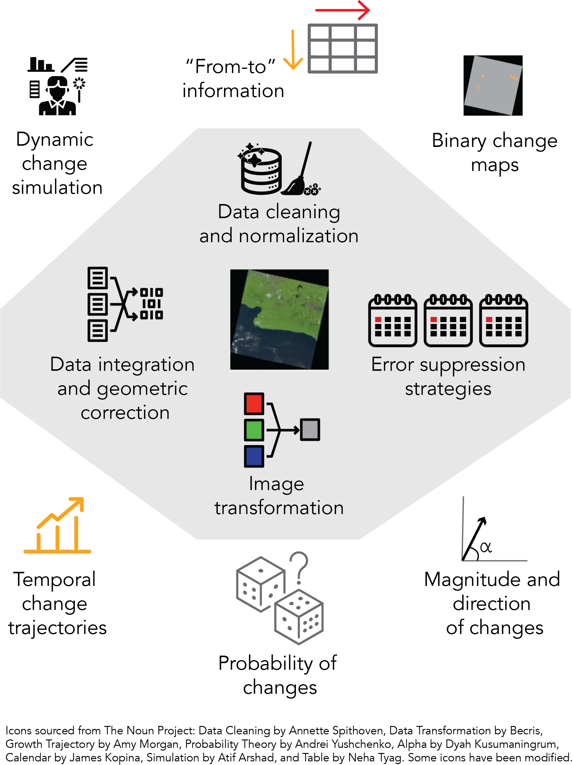
Methods	Data types	Application	References
Differencing	Landsat	Wetlands	[151]
		Savanna	[152]
		Forest	[153]
VI differencing	Landsat	Land cover	[154]
		Urban	[155]
		Forest	[156]
Differencing combined with other techniques (regression, PCA, genetic algorithm)	Landsat	Forest	[157,158]
		Land cover	[159]
Ratioing	ERS-1 SAR	Forest	[113]
	Shuttle Imaging Radar	Agriculture	[116]
	ERS, ASAR and PALSAR	Urban	[160]
Principal Component Analysis	Landsat	Land cover	[115,128]
		Urban	[161]
		Wetland	[130]
	Sentinel-2	Insect infestation	[162]
		Landslide	[163]
	Landsat and SPOT HRV	Urban	[164]
Multivariate Alteration Detection	AVHRR and Landsat	Urban	[114]
	Landsat	Forest	[69]
		Reservoir	[165]
	Quickbird	Urban	[166]
Deep-learning-based techniques	SPOT	Urban	[114]
	Worldview	Wind turbine	[149]
		Rural	[148]
	Gaofen (GF1)	Lake, river	[141]
		Buildings	[145]
	Aerial photograph	Forest	[167]

presents a summary of techniques used to derive binary change maps employing various data types applied to a range of ecosystems. The applications vary from monitoring forest to urban areas and employ either optical or radar datasets. The derived binary change maps vary in their spatial resolution from 0.5 meters (Quickbird) to 30 meters (Landsat).

4.2. Types of Change: “From-To” Information

Type of change and the composition of change are typical products of post-classification CD that relate to land cover types assigned to a unit area, such as a pixel, patch, or administrative region. Typically, post-classification change analysis generates “from-to” information, which adds the detail of change type to a binary change map [168] and can be used to understand the spatial pattern of landscape change. To obtain accurate CD, it is important to optimize classification so that error is minimized, because CD error is propagated through each classification process [169]. Meanwhile, the performance of classifiers is constrained by image type and quality, ground observations, and computational capacity [170,171,172]. Unsupervised or supervised pixel-based techniques can generate accurate CD products [171]. This section avoids discussing advances in classification algorithms themselves but focuses instead on analytical techniques and applications that generate types and composition of change.

Apart from post-classification change analysis, “from-to” information can be derived from local feature- or region-based approaches [173]. The region-based approaches have been shown to be superior for CD as compared with pixel-based approaches in terms of the following: (a) their ability to distinguish different land cover types, (b) their insensitivity to misregistration, and (c) the change of feature representation that may be well differentiated by combining texture metrics [174]. Recently developed region-based approaches include the regularized level set approach [175], faster region-based convolutional neural network (Faster R-CNN) [176], and the combined use of pixel-based and region-based approaches [177,178].

Table 2. A non-exhaustive list of methods, data source, and ecosystem applications of research that generates type or composition of change information.

Methods	Data types	Applications	References
Post-classification (various algorithms)	CASI	Invasive species	[133]
	Landsat	Land cover	[181]
		Agriculture	[188]
	Landsat and MODIS	Wetland	[189]
	Sentinel-2 and Orthophoto-map	Forest	[190]
PCA and classification	Landsat	Forest	[191]
		Urban	[161]
	Landsat and SPOT	Forest	[192]
	Landsat and Quickbird	Urban	[180]
Post-classification with other techniques	Quickbird and WorldView	Tree mortality	[179]
	Landsat	Savannah	[187]
	ADAR Hyperspectral	Urban	[40]
Region-based approaches	SPOT-5	Urbanisation	[193]
	Cartosat-1	Building and forest	[194]
Regularised level set region-based approach	Landsat	Various test site (urban, watershed)	[175]
Faster region-based convolutional neural networks	IKONOS – UAV and Gaofen-2 – Pleiades 1B	Agriculture and rural areas	[176]
Combining pixel- (classification) and region-based approaches	KVR	Mining area	[177]
	Landsat	Land cover (heterogenous area)	[178]

summarizes relevant published research according to contextual methods, data sources, and ecosystem applications used to generate change type and composition of change information. Post-classification CD is the main technique for generating type of change. The combination of post-classification techniques with other methods has improved CD sensitivity, and has improved classification accuracy [179,180]. Various classification techniques, ranging from standard unsupervised and supervised classification methods, such as k-means clustering and maximum likelihood, respectively, or more advanced methods, such as artificial intelligence or support vector machines, have been employed to achieve greater classification accuracies preceding change analysis [181,182]. Various image sources have been assessed including multispectral images with medium or high spatial resolutions and hyperspectral images from airborne or satellite platforms [40,183]. CD using SAR data has also been implemented to detect land alterations in urban and forest areas [182,184].

Numerous strategies to improve accuracy when deriving “from-to” information have been studied through employing the latest classification algorithms or by combining two or more techniques. An Iterative Compound Classification was tested in an agricultural region, and generated higher accuracy compared to post-classification analysis [185]. Although computationally expensive, other research combined change vector analysis, PCA, and temporal signature description to improve change detection accuracy for urban land cover [186]. The combination of classification techniques with PCA or with geostatistical analysis has been implemented to enhance classification accuracy and in turn increase CD accuracy [184,187].

4.3. Magnitude and Direction of Change

Other products of CD analysis are the magnitude and direction of change information, which are typically generated from change vector analysis (CVA) [195]. The products sum the information to be used for differentiating change types, which is a common reason to favor this technique. In general, the direction of change can be identified by employing two bands while the magnitude of change uses more than two spectral bands. A graphical representation of CVA was introduced by Wegmann, et al. [196] and Figure 2 presents an illustration of CVA.

Three essential prerequisites for CVA include the following: (a) precise registration, (b) preprocessing to reduce noise and stabilize performance, and (c) determining a minimum area of interest to avoid the “salt and pepper” effect [65]. According to Kontoes [197], a change vector can be defined as the angle of change.

Original image spectra or their transformations, such as indices, have been analyzed by using CVA. Transformed data such as TC [48,65,198] or vegetation indices [199] have also been used to undertake CVA. Schoppmann and Tyler [48] concluded that performing CVA on transformed images allows change process inference, particularly when obtaining ground truth information is challenging. By employing different types of data, including vegetation indices and surface reflectance, Lambin and Strahler [200] highlighted that different indicators identified different change processes. Combined application of raw spectral and transformed data was demonstrated for investigating a mountainous area by Nordberg and Evertson [158], who formulated the direction of change from the combination of Bands 3 and 4 of Landsat data, while the magnitude was determined from the three components of the TC transformation, i.e., greenness, wetness, and brightness.

CVA best suits CD within land cover classes; hence, CVA alone cannot provide the desirable “from-to” information. Johnson and Kasischke [65] highlighted the limitation of CVA for change labeling as follows: Change vectors describe change dynamics, but not states (i.e., class membership at the start and end of vectors). Defining thresholds to delineate changed from unchanged pixels is another challenge for CVA [201], particularly when dealing with multispectral images. Multispectral images are likely to be heterogeneous in their spectral bands, thus, applying a single threshold could be insufficient [202]. This issue can be overcome by normalizing the data and transforming the result into a posterior probability [201].

CVA can be used to compare the difference of biophysical indicators along a temporal trajectory, from the combination of the length of the vector, representing different magnitudes, and change direction, which indicates the nature of the change [203]. CVA is a multivariate technique since it can analyze at least two spectra. The direction of change can be used to classify change types at 2n change directions, where n equals the number of spectral bands [65], while the magnitude of change can form 3n+2 feature spaces to filter meaningful change areas [197]. CVA is most advantageous when spectral changes are unknown or when spectral variabilities are difficult to comprehend [65]. An improved version of CVA, i.e., one based on deep learning, is capable of spatially modeling correlated pixels, and has been tested for CD with three VHR images, i.e., Worldview, Quickbird, and Pleiades [204].

Various investigations have employed CVA including, but not limited to, forest areas, post-hazard change phenomena, and urban expansion.

Table 3. Research that has applied change vector analysis (CVA) as a single technique or in combination with other methods to produce magnitude and direction of change information for various ecosystems.

Methods	Data	Applications	References
CVA on image spectra or TC	Landsat	Forest and land cover	[195,198,205]
		Polluted areas	[48]
		Arid vegetation	[206]
	Landsat, Sentinel-1, Sentinel-2	Forest	[207]
CVA with various classification algorithms	Landsat	Wetland	[208]
		Land cover	[197,202]
	AVIRIS	Conserved areas	[49]
CVA with multivariate analysis	AVHRR	Desert	[203]
	MODIS	Desert, city	[199,209]
CVA with level set evolution or continuity rules	Landsat	Mountainous area	[210,211]
CVA based on deep learning	Worldview, Quickbird, Pleiades	Urban	[204]

describes examples of studies of diverse ecosystems that have applied CVA as a single technique or in combination with other approaches.

4.4. The Probability of Change

Change probability is an estimated value representing the likelihood of change in an area and is usually generated from temporal analysis of historical datasets. The identification of the probability of change enables forecasting future conditions, which is important for planning-related research.

The change probability has generally been produced using different statistical techniques following, for example, Chi-square, logistic, or Gaussian distributions. Shi and Ding [212], for instance, employed the Chi-square distribution to estimate the probability of change. The probability was derived by utilizing Bayesian probability from temporally stacked images or from binary images of differing acquisitions [213]. Examining two observations, a modified form of CVA was used to generate change probabilities [201]. They called this technique CVA in posterior probability space (CVAPS). It has the advantage of scaling the change magnitudes to a consistent range (that of posterior probabilities, zero to one), and thus requires only one threshold across classes, making optimizing the threshold more efficient as compared with CVA, which needs one threshold per class.

Estimating change probability has been implemented for multiple applications. A likelihood ratio has been used to identify the probability of flood-affected areas and vehicle distributions by using ERS-2 SAR and airborne SAR, respectively [214]. The change probability of biologically complex ecosystems was estimated, based on the proportional area of changed and unchanged lands by using multiband image difference (MID) [154]. Probability of urbanization was identified by using a Bayesian P-spline to highlight changes across time and location [215], while Wang, et al. [216] employed the scale invariant features transform (SIFT) method to calculate the probability of changed/unchanged land. Finally, coherent change detection was implemented to map the probability of volcanic ash distribution [217] and the probability of damage due to natural disaster [218].

Some researchers have demonstrated the use of change probabilities while identifying driving forces of change. Employing various regression techniques, the likelihood of change can be estimated by considering the contribution of determinant factors from multiple variables. An example of this employed generalized linear models (GLMs) and semi-variograms to judge the importance of change metrics and produced probability of change and variability of change images [219]. Logistic regression is a frequently used technique for determining driving forces of change; for instance, the identification of change determinants while estimating change likelihood of a pixel [220], the determination of reforestation probability [221], and quantification of forest degradation probability based on biophysical and socioeconomic datasets [222].

The probability of change can also inform error detection rates including the error and false alarm probabilities [223]. Despite being able to highlight the most probable locations of false alarms, local estimates of error probability were not calculated in that article. Other research by Cartus, et al. [224] investigated the change detection error probability during an investigation of forest cover loss by using L-band backscatter.

Integrating evidential information can improve the accuracy of change information or likelihood of CD. The Dempster–Shafer theory is generally the basis of evidential fusion [225], which was implemented to integrate images from several optical satellites [226,227], airborne laser scanners [228], and SAR images or a combination of optical and SAR images [229]. A modified version of Dempster–Shafer, the dynamic evidential reasoning method, was proposed for sequential image fusion to deal with the changing frame of different images [230]. The theory has been implemented for studies with a range of aims, for example, to update a building map [229], to detect landslides [231], and to detect newly built-up areas [232].

4.5. Temporal Change Trajectories

A land use and cover change (LUCC) trajectory can be defined as the periodically observed temporal sequence of a pixel’s land cover that is integrated in serial datasets [111]. The LUCC trajectory change detection (TCD) can also be seen as a temporal development curve that could be generated from multitemporal images [203]. The use of multitemporal datasets improves sensitivity to seasonal, gradual, or subtle changes. Then, trends can be identified from the sequence of change to highlight the dynamic character of change [233,234].

The availability of freely accessible image archives and the insensitivity of bitemporal analysis to describe the dynamics of sub-annual changes have driven advances in trajectory change analysis. Space agencies have administered programs to support monitoring global land cover by providing free data from NASA and USGS’s Landsat and through the ESA’s Sentinel program. Freely accessible data such as AVHRR, MODIS, SPOT, and PROBA accelerated the development of techniques and algorithms, as well as applications that allow further investigation of global temporal LUCC dynamics [235].

Change trajectories can be analyzed from either periodical or nonperiodical datasets. Frequent periodical observations have distinctive advantages, such as the capability to indicate either temporary or permanent change processes and the start and end of growing seasons [236,237]. This sort of information is crucial for monitoring management practices, to investigate the intensity of land use or climatic conditions, or changes in the way that land is being used. The use of remote sensing indices for TCD was introduced by Lambin and Strahler [203], who employed vegetation indices and land surface temperatures. Temporal trajectories of indices indicate the cause of change processes and record alterations over time [4]. Temporal patterns can also be used to estimate disturbances [238]. Trends assist in understanding influential factors of LUCC [239] or understanding seasonal dynamics [240], which cannot be portrayed in bitemporal observations. In most cases, the study of temporal trajectories has employed statistical analysis, particularly, time series analysis.

Descriptive or statistical time series analysis (TSA) can be implemented for TCD. Descriptive analyses employ any number of observations while statistical TSA strictly requires frequent, periodical, observable facts [241]. Indeed, there are various interpretations of TSA applied in remote sensing. For instance, according to Giri, et al. [242], TSA refers to multitemporal analysis of images to represent two seasons, i.e. summer and harvest, whereas for Jonsson and Eklundh [237], TSA implies a statistical time series approach to studying seasonal dynamics. The use of statistical time series in remote sensing aids in understanding general trends and seasonal dynamics of change from sub-annual observations. The following sections discuss techniques focusing on change detection particularly on trend and seasonal dynamics.

4.5.1. Temporal Trend

Trend is a parameter that can be derived either from temporally periodical or nonperiodical observations. Trends from nonperiodical observations are generally obtained from aggregate information such as annual or any periodically aggregated observations. In land-cover-related research, a change in trend can indicate disturbances [243]. Curve fitting is an alternative to nonperiodical techniques to analyze trends. A hypothetical curve pattern is often used to evaluate the trend of LCC phenomena [233,244]. Hüttich, et al. [245] employed annual data derived from SPOT mosaics to investigate the trend of vegetation green-up in the boreal forest zone, while Zhou [246] quantified trajectory changes using landscape metrics. Common statistical techniques such as regression, can be utilized to estimate trend parameters. Xue, et al. [247] implemented curve fitting to investigate the trajectory of change before ingesting images into classification algorithms.

Trend parameters can be gathered from seasonal observations through deseasonalizing data or by employing stationary or nonstationary decomposition techniques [243,248,249]. The assumption of stationary temporal patterns can limit implementing these techniques to phenomena with particular temporal change characteristics. Abrupt changes that drastically deviate from a temporal curve of biophysical properties, such as those induced by natural events such as volcanic explosions, floods or fires, do not meet the stationarity criterion.

Table 4. Major time series decomposition techniques for LCC-related studies.

Method	Abbreviation	Description	References
Seasonal Time Series Analysis based on loess regression	STL	Decomposing time series of spectral bands into three components, i.e., trend, seasonal and remainder.	[250,251]
Fourier transform	FT	Decomposing time series of spectral bands by using superposition of sine and cosine functions.	[252,253]
Singular Spectrum Analysis	SSA	Decomposing time series of spectral bands into different oscillatory components without fitting.	[254,255]
Wavelet transform	WT	Decomposing time series into linear combinations of wavelet function.	[256,257]
Seasonal trend analysis	STA	Harmonic analysis to extract annual and semi-annual time series harmonics.	[258]
Landsat-based detection of trends in disturbances and recovery	LandTrendR	Extracting spectral trajectories of land surface change from yearly Landsat time series stacks.	[259]
Break for Additive Season and Trend	BFAST	Integrating decomposition of time series data with the capacity to detect change within the time series.	[243]
Auto-regressive Integrated Moving Average	ARIMA	Univariate time series that may transform nonstationary data series into stationary models through differencing.	[260,261]
Seasonal Autoregressive Integrated Moving Average	SARIMA	Similar model to ARIMA but involving backshift of seasonal period.	[262]
X12-Autoregressive Integrated Moving Average	X12-ARIMA	Seasonal adjustment of univariate time series models that decomposes spectral bands into seasonal-trend-irregular components.	[263,264,265]
Ensemble Empirical Mode Decomposition	EEMD	Decomposing satellite image time series into intrinsic mode functions (IMFs) and selecting relevant IMFs to separate trend and seasonal components.	[266,267,268]
–Detecting Breakpoints and estimating segment in trend	DBEST	A segmentation algorithm that simplifies the trend into linear segments employing three parameters including a generalisation threshold, the largest changes and the magnitude of change.	[269]
Sub-annual Change Detection	SCD	Detecting abrupt land cover change from sub-annual scale.	[270]
Change, After Effect and Trend	CAT	Suppressing seasonal effects to identify change, after effect, and trend.	[271]

summarizes the major decomposition techniques used to detect LCC and provides a short description about the techniques, sorted from older to newer applications in remote sensing-related research.

Break for additive season and trend (BFAST) is the most widely employed technique for remote sensing time series analysis amongst the decomposition techniques. BFAST is a modified technique for seasonal time series analysis based on loess regression, and was introduced by Cleveland, Cleveland and Terpenning [250]. BFAST combines a harmonic seasonal model and ordinary least squares analysis based on a moving sum (OLS-MOSUM) test which can detect the breakpoints occurring within a serial dataset through an additive decomposition model [243].

Table 5. Varying image revisit times and observation targets implementing BFAST.

Datasets	Periodical/Number of Observations (Scenes)	Observation Targets	References
Landsat	16-day	Combining time series data for LUCC	[272]
	Irregular/55	Small-scale forest disturbances	[273]
	Irregular/270	Forest disturbances	[274]
	Iregular/(135, 104, 94)	Error generation of forest change	[275]
	Irregular/94	Forest disturbances	[276]
MODIS vegetation	16-day	Exploring change within near observed data/deforestation	[277,278]
		Response of vegetation to flood and fire	[279]
		Phenology-based classification	[247]
		Characterising vegetation dynamics	[280,281]
		The impact of confining elephants in a forest on land use change	[282]
		Biomass estimation	[283]
MODIS reflectance	8-day	Identifying LCC that corresponded to urban expansion	[284]
SPOT vegetation	10-day	Estimating water balance variables	[285]
Sentinel-2	5-day	Monitoring agricultural parcels	[286]
The combination of several images	unstated	Fire-induced changes	[223]
		Improving deforestation monitoring	[287]
Simulated data	unstated	Comparing time series models	[288]

presents the implementation of BFAST for different remote sensing-based analyses. The table shows that various periodical observations have been applied in different studies. Most of these studies employed MODIS and Landsat data, while a few studies used SPOT or other platforms. The studies mostly employed vegetation indices, such as NDVI and Enhanced Vegetation Index (EVI). Moreover, the majority of BFAST implementations were directed to understanding deforestation and forest disturbances.

4.5.2. Seasonal Pattern

In general, time series methods decompose a signal into three components, i.e., trend, seasonal, and irregular, to reveal several change phenomena. Seasonal trend decomposition based on loess (STL) and seasonal trend analysis (STA) are amongst the decomposition techniques that have been implemented in remote sensing studies [250]. Many investigations of temporal trajectories focus on detecting seasonal patterns of change dynamics [237,243,258]. Since indices serve as the primary data source, selection of proper indices influences the capabilities of STA.

The incorporation of a seasonality adjustment should be considered, since most time series remote sensing applications employ reflectance or indices that are affected by season. Seasonality is defined as the amplitude of the temporal profile of indices to indicate photosynthetic activity of vegetation [289]. Seasonality metrics can be estimated by using statistical time series such as the beginning and end of seasons, the number of growing seasons, or the rates of growth and decline [237]. The metrics have been employed to discriminate the phenology of different vegetation types and the intensity of agricultural cultivation within a year.

STL is capable of differentiating areas with annual vegetation from those with perennial vegetation [251]. The idea was first introduced by Cleveland, Cleveland and Terpenning [250] and was applied to understand air quality based on remote sensing observations [250] and to map seasonal variation of vegetation [290]. A later version of STL, namely STA, uses harmonic equations capable of extracting annual and semi-annual harmonics [258]. Carrao, et al. [291] showed that STA could be used to estimate the near future of earth-surface characteristics, such as vegetation greenness or temperature. The combination of STA to extract seasonal parameters and PCA to contrast changed and unchanged places was found to be beneficial for characterizing many types of land cover transition [292]. A further extension of STA, seasonal trend analysis and segmentation to detect land cover (SDTC), allows multiple variables to be combined [293]. The significance of temporal trend was tested by using the Mann–Kendall procedure and it appeared to be valuable in detecting and characterizing land cover change.

TIMESAT is a popular tool for investigating seasonal patterns. With optional distributions of asymmetric Gaussian, Savitsky–Golay, double logistic function, or nonlinear least square fits, this tool was used to define seasonality parameters, including intensity of growth, the beginning and end of a season, and growth rate [237]. The tool provides smoothed, meaningful data derived from remote sensing images [294]; applications of this tool are summarized in

Table 6. Remote sensing investigations employing TIMESAT.

Datasets	Temporal Revisit	Objectives	References
AVHRR	10-day	Seasonality metrics extraction	[237]
		The trend of VI	[295]
		Phenological change	[296,297]
		Exploring anthropogenic and climate effects on vegetation	[298]
	Monthly	Phenological metrics and productivity extraction	[299]
		Assessing land degradation/recovery	[300]
MODIS Vegetation Index	16-day	The extraction of phenological metrics for: - rice crops	[301]
		- forest	[302]
		- vegetation affected by insect infestation	[303]
		- abandoned agriculture	[304]
		- complex ecosystems	[305]
		- spring ephemerals	[306]
		Mapping seasonality metrics	[307]
MODIS Surface Reflectance	8-day	Improving ecosystem classification	[302]
		Mapping fractional forest cover	[308]
		Tracking seasonal change in coniferous forest	[309]
		Monitoring cotton stages	[310]
		Delineating vegetation phenology	[311]
		Ecosystem assessment	[312]
		Validating spring green-up	[313]
MODIS LAI	8-day	Smoothing and gap-filling data	[314]
		Modelling land surface and climate	[315]
MERIS	10-day	Estimating start of season (SOS)	[316]
		Extracting phenological information for deciduous forest	[317]
AMSR-E	4-day	Estimating SOS and ecoregion variability	[318]
HJ-1 data	Irregular	Estimating crop phenology	[319]
PROBA-V	Daily	Mapping peanut cultivation	[320]
SPOT-4	5-day	Scheduling irrigation	[321]
Sentinel-2	5-day	Mapping macrophyte phenology at a lake	[322]
Combination of various sensors	8-day	Studying deciduous forest carbon flux	[323]
	16-day	Impact of illumination on seasonal metrics	[324]
	5-day	Exploring macrophyte seasonal dynamics	[322]

. In general, the table indicates a variety of data types, temporal revisit intervals, and objectives or ecosystem applications that have applied TIMESAT. The data sources include medium to coarse spatial resolution optical images, such as AVHRR, MODIS, MERIS, SPOT vegetation, and PROBA, as well as coarse microwave images such as AMSR-E. Combining images has also been used to improve the interpretation of seasonal changes and their drivers.

4.6. Dynamic Simulation of Changes

Simulation of future land cover changes has been an interest of many remote sensing users for land and ecosystem monitoring, management, and planning. The topic has been discussed widely, often by integrating the concepts of remote sensing and GIS or spatial analysis [325]. Temporal interpolation is usually employed in a simulation, whereas spatial interpolation has been applied with stricter assumptions. The integration of temporal and spatial models allows the understanding of complex systems and their spatiotemporal dynamics [326].

Various techniques for dynamic simulation have been developed in the areas of geoscience and ecosystem modeling. The Conversion of Land Use and its Effect (CLUE) model [327] and cellular automata principles [328], have been implemented for dynamic modeling of various ecosystems contexts. In another case, Bacani, et al. [329] combined a Markov chain model and cellular automata to generate spatiotemporal change probability maps for wetlands. A supervised classification using a multilayer perceptron (MLP), a type of Markov chain model, was implemented to predict land cover change in a semiarid area [330]. Markov chain models, however, have been criticized regarding their ability to detect errors since the drivers of change are omitted. This drawback can be minimized by employing binary logistic regression to determine the drivers of change for future simulations by artificial neural networks (ANN) [331]. Comparing parametric and non-parametric models for simulating land use change, Tayyebi, et al. [332] demonstrated that ANNs outperformed two other non-parametric models, classification and regression tree (CART) and multivariate adaptive regression splines (MARS), to estimate short time intervals of coarse spatial resolution data.

5. Accuracy Assessment of Change Detection Techniques

Accuracy assessment is required for affirming reliable information and for evaluating the robustness of classification or segmentation techniques. Common accuracy assessment is based on an error matrix or confusion table [333], which identifies overall accuracy, false positive/commission errors, and false negative/omission errors. A few references described false positives as false alarms and false negatives as missed alarms/detections [157,334]. Some approaches have also been proposed to assess change detection accuracy, such as the change detection error matrix [169], area-based accuracy [335], accuracy assessment curve [336], and rule-based rationality [333]. The manageability of the error matrix was questioned when dealing with more than two images for change analyses, therefore Li and Zhou [337] proposed a trajectory error matrix for change analysis involving more than two images. Since not all of the assessments have been examined in various settings, the robustness of the techniques within differing environments needs to be investigated in the future.

Accuracy has been reported to be the result of many factors, including image properties and the seasonal condition affecting the quality of images [338], preprocessing being involved for aligning or correcting the quality of the images [60]; correlation among spectral bands and among image pairs; sampling strategies [339]; and techniques for generating change information. When classification or segmentation techniques were involved, the accuracy of change detection depended upon single date accuracies and was commonly calculated as the product of these [340]. Nonetheless, Congalton and Green [341] argued that correlation among layers contributed to the accuracy, where the sum product would be relevant for independent classified layers, whereas correlated layers would relate to single-date accuracy.

6. Challenges, Comparisons, and Future Directions for CD Techniques

The primary challenge for applying bitemporal techniques lies in the decision strategy used to separate changed from unchanged land. A common strategy is to employ the mean and standard deviation of features to determine thresholds for differencing, ratioing, and PCA with various ranges of constants [126,154,342,343,344]. Meanwhile, a hypothetical range was applied for thresholding by determining 10% of the proportion as change [129], employing Bayes theory [345,346], or the Wishart distribution [347] for automatic thresholding. It appears that advances in binary change detection go beyond simple algebra techniques. The integration of relative radiometric corrections in a simultaneous manner, such as in MAD, offers a robust yet efficient procedure to generate binary change maps. Similarly, ISFA offers normalization while applying unsupervised change detection. Meanwhile, various deep-learning-based techniques have recently been developed for unsupervised change detection and tested in several settings. Nonetheless, the effectiveness of these methods for monitoring regional or global extent needs to be explored.

A different challenge applies for post-classification change analysis. The selection of suitable classifiers is essential to optimize accuracy, meanwhile, particular sampling strategies such as cross-validation or tuning parameters can improve the performance of classifiers [348]. Various strategies have been proposed for cross-validation for simultaneous change detection, such as by using a generative adversarial network to optimize change detection based on min-max game theory [349] or using a learning algorithm called iterative active learning to define multitemporal training sets [350]. Subtle changes related to spatial resampling, land management, and vegetation species or vegetation growth stages are understudied. However, a few such examples were found, for instance, a combination between IRMAD and random forest classification of amended SAR images with polarimetric decomposition layers to detect subtle change related to vegetation growth stages in cloud-prone regions [351].

Employing multiple sensors and spatial resolutions for long temporal analysis is the consequence of sensors’ limited lifetimes. The consequence is well known; yet, a paucity of research related to sensor compatibility is evident in the literature. Meanwhile, trajectory change detection employing time series datasets needs to adapt to different properties of datasets. The exploration of techniques for relative radiometric corrections becomes more important for applications employing massive and temporally continuous observations.

Detecting changes at the subpixel level can now be undertaken, allowing the investigation of detailed aspects of land cover when access to high resolution imagery is limited. Employing subpixel techniques outperformed traditional techniques in terms of analyzing images with different spatial resolutions [213] or inspecting subpixel image features [352].

The development of techniques, algorithms, and tools has facilitated the investigation of change for bitemporal and trajectory analyses, and simulation of future changes. R-based algorithms enable such analyses using a number of libraries for change detection, ranging from preprocessing such as geometric, radiometric, and atmospheric corrections; bitemporal change detection methods such as CVA; to seasonal time series analysis such as BFAST, DBEST, STA, STL, ARIMA, and X12-ARIMA [353]. Tools implemented in software packages other than R are also available from respected researchers, for instance, the IDL-based tools such as IRMAD for bitemporal CD [354] or TiSeG for MODIS quality assessment [44,355], and TIMESAT for seasonal time series analysis based on Fortran/MATLAB [294]. Meanwhile, more available image archives and the recent Copernicus program are likely to motivate more participation in and development of tools for global monitoring of land cover changes.

In addition to the development of novel algorithms, the combination of available techniques is being considered to improve CD accuracy. Silveira, Mello, Acerbi Júnior and Carvalho [187], for instance, combined differencing and geo-statistical parameters for segmentation preceding CD. Differencing, masking, and multivariate clustering were combined to detect tree mortality in mixed-species woodlands [179]. An improved Kappa has been obtained by combining CVA, PCA, and temporal signature description [186]. Moreover, an advanced version of CVA, called compressed CVA, can perform change probability estimation [356]. Another strategy that combines multiple sources of evidence by employing Dempster–Shafer Theory could be an option for analyzing changes utilizing various images [227].

Characterization and attribution of changes have been implemented to improve interpretation of change processes [357]. Spectral mixture analysis (SMA) is a model to separate a variable into wavelength-independent and -dependent components [358]. The model has been applied to discriminate soil, rock, shade, and the secondary illumination effects using Viking Lander imagery [358].

To sum up, various land cover change processes require suitable techniques for synoptic yet seamless monitoring. Remote sensing is a fast-moving field, and new techniques keep emerging and these topics are a key area for global monitoring. Considering the need to understand interrelations among ecosystem components, understanding complex models is undoubtedly be even more relevant in the future. Beyond 2D change detection, the 3D detections will also be valuable. Contextual research on land cover change and its effects should include drivers of change, and the prediction of location and quantity of changes [359]. The use of ancillary data from various sources, instead of merely relying on remotely sensed data, has been practical for assisting the interpretation of complex change processes and indicating relevant stressors. It appears that integrating several methods and datasets should become the standard of analysis in the future.

The acceleration of change globally driven by naturogenic and anthropogenic factors creates greater variability of change processes. Hence, bitemporal, multitemporal, and time series techniques are needed to enable the investigation of heterogenous change types, intensities, and process durations, as well as to suit the diverse purposes of studies. The era of freely accessible data in parallel with the growth of non-proprietary toolboxes should propagate doubly through remote sensing communities, as well as users.

References

- Singh, A. Review Article: Digital Change Detection Techniques Using Remotely-Sensed Data. Int. J. Remote Sens. 1989, 10, 989–1003. [Google Scholar] [CrossRef]
- Bruzzone, L.; Bovolo, F. A Novel Framework for the Design of Change-Detection Systems for Very-High-Resolution Remote Sensing Images. Proc. IEEE 2013, 101, 609–630. [Google Scholar] [CrossRef]
- Radke, R.J.; Andra, S.; Al-Kofahi, O.; Roysam, B. Image change detection algorithms: A systematic survey. IEEE Trans. Image Process. 2005, 14, 294–307. [Google Scholar] [CrossRef]
- Mouat, D.A.; Mahin, G.G.; Lancaster, J. Remote sensing techniques in the analysis of change detection. Geocarto Int. 1993, 8, 39–50. [Google Scholar] [CrossRef]
- Ingram, K.; Knapp, E.; Robinson, J. Change Detection Technique Development for Improved Urbanized Area Delineation; CSC/TM-81/6087; NASA, Comput. Sci. Corp.: Springfield, MD, USA, 1981.
- Ban, Y.; Yousif, O. Change detection techniques: A review. In Remote Sensing and Digital Image Processing; Springer International Publishing: Cham, Switzerland, 2016; pp. 19–43. [Google Scholar]
- Coppin, P.; Jonckheere, I.; Nackaerts, K.; Muys, B.; Lambin, E. Digital change detection methods in ecosystem monitoring: A review. Int. J. Remote Sens. 2004, 25, 1565–1596. [Google Scholar] [CrossRef]
- Nelson, R.F. Detecting Forest Canopy Change Due to Insect Activity Using Landsat Mss. Photogramm. Eng. Remote Sens. 1983, 49, 1303–1314. [Google Scholar]
- Lu, D.; Mausel, P.; Brondízio, E.; Moran, E. Change detection techniques. Int. J. Remote Sens. 2004, 25, 2365–2401. [Google Scholar] [CrossRef]
- Hussain, M.; Chen, D.M.; Cheng, A.; Wei, H.; Stanley, D. Change detection from remotely sensed images: From pixel-based to object-based approaches. ISPRS J. Photogramm. Remote Sens. 2013, 80, 91–106. [Google Scholar] [CrossRef]
- Bovolo, F.; Bruzzone, L. The Time Variable in Data Fusion: A Change Detection Perspective. IEEE Geosci. Remote Sens. Mag. 2015, 3, 8–26. [Google Scholar] [CrossRef]
- Rosenqvist, Å.; Milne, A.K.; Lucas, R.; Imhoff, M.; Dobson, C. A review of remote sensing technology in support of the Kyoto Protocol. Environ. Sci. Policy 2003, 6, 441–455. [Google Scholar] [CrossRef]
- Rosenqvist, Å. Systematic data acquisitons—A pre-requisite for meaningful biophysical parameter retrieval? In Proceedings of the Third International Symposium on Retrieval of Bio- and Geophysical Parameters from SAR Data for Land Applications, Sheffield, UK, 11–14 September 2001. [Google Scholar]
- Lauer, D.T.; Morain, S.A.; Salomonson, V.V. The Landsat program: Its origins, evolution, and impacts. Photogramm. Eng. Remote Sens. 1997, 63, 831–838. [Google Scholar]
- Roy, D.P.; Wulder, M.A.; Loveland, T.R.; Woodcock, C.E.; Allen, R.G.; Anderson, M.C.; Helder, D.; Irons, J.R.; Johnson, D.M.; Kennedy, R.; et al. Landsat-8: Science and product vision for terrestrial global change research. Remote Sens. Environ. 2014, 145 (Suppl. C), 154–172. [Google Scholar] [CrossRef]
- Yamaguchi, Y.; Fujisada, H.; Kudoh, M.; Kawakami, T.; Tsu, H.; Kahle, A.B.; Pniel, M. ASTER instrument characterization and operation scenario. Adv. Space Res. 1999, 23, 1415–1424. [Google Scholar] [CrossRef]
- Rosenqvist, A.; Shimada, M.; Watanabe, M.; Tadono, T.; Yamauchi, K. Implementation of systematic data observation strategies for ALOS PALSAR, PRISM and AVNIR-2. In Proceedings of the IEEE International Geoscience and Remote Sensing Symposium 2004, Anchorage, AK, USA, 20–24 September 2004. [Google Scholar]
- Vollmar, M.; Rasi, R.; Beuchle, R.; Simonetti, D.; Stibig, H.-J.; Achard, F. Combining Landsat TM/ETM+ and ALOS AVNIR-2 satellite data for tropical forest cover change detection. IEEE J. Sel. Top. Appl. Earth Obs. Remote Sens. 2013, 6, 102–109. [Google Scholar] [CrossRef]
- Im, J.; Jensen, J.R.; Hodgson, M.E. Optimizing the binary discriminant function in change detection applications. Remote Sens. Environ. 2008, 112, 2761–2776. [Google Scholar] [CrossRef]
- Witmer, F.D.W. Detecting war-induced abandoned agricultural land in northeast Bosnia using multispectral, multitemporal Landsat TM imagery. Int. J. Remote Sens. 2008, 29, 3805–3831. [Google Scholar] [CrossRef]
- Ardila, J.P.; Bijker, W.; Tolpekin, V.A.; Stein, A. Quantification of crown changes and change uncertainty of trees in an urban environment. ISPRS J. Photogramm. Remote Sens. 2012, 74, 41–55. [Google Scholar] [CrossRef]
- Uddin, K.; Gilani, H.; Murthy, M.S.R.; Kotru, R.; Qamer, F.M. Forest Condition Monitoring Using Very-High-Resolution Satellite Imagery in a Remote Mountain Watershed in Nepal. Mt. Res. Dev. 2015, 35, 264–277. [Google Scholar] [CrossRef]
- Huang, X.; Zhu, T.; Zhang, L.; Tang, Y. A novel building change index for automatic building change detection from high-resolution remote sensing imagery. Remote Sens. Lett. 2014, 5, 713–722. [Google Scholar] [CrossRef]
- Li, P.; Song, B.; Xu, H. Urban building damage detection from very high resolution imagery by One-Class SVM and shadow information. In Proceedings of the International Geoscience and Remote Sensing Symposium (IGARSS), Vancouver, BC, Canada, 24–29 July 2011. [Google Scholar]
- Berger, M.; Moreno, J.; Johannessen, J.A.; Levelt, P.F.; Hanssen, R.F. ESA’s sentinel missions in support of Earth system science. Remote Sens. Environ. 2012, 120, 84–90. [Google Scholar] [CrossRef]
- Drusch, M.; Del Bello, U.; Carlier, S.; Colin, O.; Fernandez, V.; Gascon, F.; Hoersch, B.; Isola, C.; Laberinti, P.; Martimort, P.; et al. Sentinel-2: ESA’s Optical High-Resolution Mission for GMES Operational Services. Remote Sens. Environ. 2012, 120, 25–36. [Google Scholar] [CrossRef]
- Fensholt, R.; Rasmussen, K.; Nielsen, T.T.; Mbow, C. Evaluation of earth observation based long term vegetation trends—Intercomparing NDVI time series trend analysis consistency of Sahel from AVHRR GIMMS, Terra MODIS and SPOT VGT data. Remote Sens. Environ. 2009, 113, 1886–1898. [Google Scholar] [CrossRef]
- Whittle, M.; Quegan, S.; Uryu, Y.; Stüewe, M.; Yulianto, K. Detection of tropical deforestation using ALOS-PALSAR: A Sumatran case study. Remote Sens. Environ. 2012, 124, 83–98. [Google Scholar] [CrossRef]
- Fily, M.; Rothrock, D.A. Sea ice tracking by nested correlations. IEEE Trans. Geosci. Remote Sens. 1987, GE-25, 570–580. [Google Scholar] [CrossRef]
- Martinis, S.; Twele, A.; Voigt, S. Unsupervised extraction of flood-induced backscatter changes in SAR data using markov image modeling on irregular graphs. IEEE Trans. Geosci. Remote Sens. 2011, 49 Pt 1, 251–263. [Google Scholar] [CrossRef]
- Martinis, S.; Rieke, C. Backscatter analysis using multi-temporal and multi-frequency SAR data in the context of flood mapping at River Saale, Germany. Remote Sens. 2015, 7, 7732–7752. [Google Scholar] [CrossRef]
- ESRI. GIS Dictionary. Available online: https://support.esri.com/en/other-resources/gis-dictionary/term/3857589e-6985-4b73-8eba-08682aa5cad7 (accessed on 29 March 2020).
- Franklin, J. Predictive vegetation mapping: Geographic modelling of biospatial patterns in relation to environmental gradients. Prog. Phys. Geogr. 1995, 19, 474–499. [Google Scholar] [CrossRef]
- Rogan, J.; Miller, J.; Stow, D.A.; Franklin, J.; Levien, L.; Fischer, C. Land-cover change monitoring with classification trees using Landsat TM and ancillary data. Photogramm. Eng. Rem Sens. 2003, 69, 793–804. [Google Scholar] [CrossRef]
- Hayes, D.J.; Sader, S.A. Comparison of change-detection techniques for monitoring tropical forest clearing and vegetation regrowth in a time series. Photogramm. Eng. Remote Sens. 2001, 67, 1067–1075. [Google Scholar]
- Oetter, D.R.; Cohen, W.B.; Berterretche, M.; Maiersperger, T.K.; Kennedy, R.E. Land cover mapping in an agricultural setting using multiseasonal Thematic Mapper data. Remote Sens. Environ. 2001, 76, 139–155. [Google Scholar] [CrossRef]
- Hepinstall-Cymerman, J.; Coe, S.; Alberti, M. Using urban landscape trajectories to develop a multi-temporal Land cover database to support ecological modeling. Remote Sens. 2009, 1, 1353–1379. [Google Scholar] [CrossRef]
- Treitz, P.; Howarth, P. Integrating spectral, spatial, and terrain variables for forest ecosystem classification. Photogramm. Eng. Remote Sens. 2000, 66, 305–318. [Google Scholar]
- Röder, A.; Hill, J.; Duguy, B.; Alloza, J.A.; Vallejo, R. Using long time series of Landsat data to monitor fire events and post-fire dynamics and identify driving factors. A case study in the Ayora region (eastern Spain). Remote Sens. Environ. 2008, 112, 259–273. [Google Scholar]
- Im, J.; Jensen, J.R. A change detection model based on neighborhood correlation image analysis and decision tree classification. Remote Sens. Environ. 2005, 99, 326–340. [Google Scholar] [CrossRef]
- Desclée, B.; Bogaert, P.; Defourny, P. Forest change detection by statistical object-based method. Remote Sens. Environ. 2006, 102, 1–11. [Google Scholar] [CrossRef]
- Hassan, M.M.; Nazem, M.N.I. Examination of land use/land cover changes, urban growth dynamics, and environmental sustainability in Chittagong city, Bangladesh. Environ. Dev. Sustain. 2016, 18, 697–716. [Google Scholar] [CrossRef]
- García, S.; Luengo, J.; Herrera, F. Data Preparation Basic Models. In Data Preprocessing in Data Mining; García, S., Luengo, J., Herrera, F., Eds.; Springer International Publishing: Cham, Switzerland, 2015; pp. 39–57. [Google Scholar]
- Panuju, D.R.; Paull, D.J.; Griffin, A.L. Spatio-temporal quality distribution of MODIS vegetation collections 5 and 6: Implications for forest-non-forest separability. Int. J. Remote Sens. 2020, 41, 373–397. [Google Scholar] [CrossRef]
- Yang, X.; Lo, C.P. Relative radiometric normalization performance for change detection from multi-date satellite images. Photogramm. Eng. Remote Sens. 2000, 66, 967–980. [Google Scholar]
- Hall, F.G.; Strebel, D.E.; Nickeson, J.E.; Goetz, S.J. Radiometric rectification: Toward a common radiometric response among multidate, multisensor images. Remote Sens. Environ. 1991, 35, 11–27. [Google Scholar] [CrossRef]
- Richards, J.A. Thematic mapping from multitemporal image data using the principal components transformation. Remote Sens. Environ. 1984, 16, 35–46. [Google Scholar] [CrossRef]
- Schoppmann, M.W.; Tyler, W.A. Chernobyl revisited: Monitoring change with change vector analysis. Geocarto Int. 1996, 11, 13–27. [Google Scholar] [CrossRef]
- Allen, H.; Simonson, W.; Parham, E.; Santos, E.B.; Hotham, P. Satellite remote sensing of land cover change in a mixed agro-silvo-pastoral landscape in the Alentejo, Portugal. Int. J. Remote Sens. 2018, 39, 4663–4683. [Google Scholar] [CrossRef]
- Kennedy, R.E.; Cohen, W.B. Automated designation of tie-points for image-to-image coregistration. Int. J. Remote Sens. 2003, 24, 3467–3490. [Google Scholar] [CrossRef]
- Song, D.X.; Huang, C.; Sexton, J.O.; Channan, S.; Feng, M.; Townshend, J.R. Use of landsat and corona data for mapping forest cover change from the mid-1960s to 2000s: Case studies from the eastern united states and central brazil. ISPRS J. Photogramm. Remote Sens. 2014, 103, 81–92. [Google Scholar] [CrossRef]
- Ayoub, F.; Leprince, S.; Avouac, J.-P. Co-registration and correlation of aerial photographs for ground deformation measurements. ISPRS J. Photogramm. Remote Sens. 2009, 64, 551–560. [Google Scholar] [CrossRef]
- Klaric, M.N.; Claywell, B.C.; Scott, G.J.; Hudson, N.J.; Sjahputera, O.; Li, Y.H.; Barratt, S.T.; Keller, J.M.; Davis, C.H. GeoCDX: An Automated Change Detection and Exploitation System for High-Resolution Satellite Imagery. IEEE Trans. Geosci. Remote Sens. 2013, 51, 2067–2086. [Google Scholar] [CrossRef]
- Jabari, S.; Zhang, Y. Building change detection using multi-sensor and multi-view-angle imagery. In Proceedings of the IOP Conference Series: Earth and Environmental Science, Halifax, Canada, 5–9 October 2015. [Google Scholar]
- Leprince, S.; Barbot, S.; Ayoub, F.; Avouac, J.P. Automatic and precise orthorectification, coregistration, and subpixel correlation of satellite images, application to ground deformation measurements. IEEE Trans. Geosci. Remote Sens. 2007, 45, 1529–1558. [Google Scholar] [CrossRef]
- Nuth, C.; Kääb, A. Co-registration and bias corrections of satellite elevation data sets for quantifying glacier thickness change. Cryosphere 2011, 5, 271–290. [Google Scholar] [CrossRef]
- Theiler, J.; Wohlberg, B. Local Coregistration Adjustment for Anomalous Change Detection. IEEE Trans. Geosci. Remote Sens. 2012, 50, 3107–3116. [Google Scholar] [CrossRef]
- Verbyla, D.; Boles, S. Bias in land cover change estimates due to misregistration. Int. J. Remote Sens. 2000, 21, 3553–3560. [Google Scholar] [CrossRef]
- Townshend, J.R.G.; Justice, C.O.; Gurney, C.; McManus, J. The impact of misregistration on change detection. IEEE Trans. Geosci. Remote Sens. 1992, 30, 1054–1060. [Google Scholar] [CrossRef]
- Dai, X.L.; Khorram, S. The effects of image misregistration on the accuracy of remotely sensed change detection. IEEE Trans. Geosci. Remote Sens. 1998, 36, 1566–1577. [Google Scholar]
- Roy, D.P. The impact of misregistration upon composited wide field of view satellite data and implications for change detection. IEEE Trans. Geosci. Remote Sens. 2000, 38, 2017–2032. [Google Scholar] [CrossRef]
- Gong, P.; Le Drew, E.F.; Miller, J.R. Registration-noise reduction in difference images for change detection. Int. J. Remote Sens. 1992, 13, 773–779. [Google Scholar] [CrossRef]
- Paolini, L.; Grings, F.; Sobrino, J.; Jiménez Muñoz, J.C.; Karszenbaum, H. Radiometric correction effects in Landsat multi-date/multi-sensor change detection studies. Int. J. Remote Sens. 2006, 27, 685–704. [Google Scholar] [CrossRef]
- Teillet, P. Image correction for radiometric effects in remote sensing. Int. J. Remote Sens. 1986, 7, 1637–1651. [Google Scholar] [CrossRef]
- Johnson, R.D.; Kasischke, E. Change vector analysis: A technique for the multispectral monitoring of land cover and condition. Int. J. Remote Sens. 1998, 19, 411–426. [Google Scholar] [CrossRef]
- Roy, D.P.; Borak, J.S.; Devadiga, S.; Wolfe, R.E.; Zheng, M.; Descloitres, J. The MODIS Land product quality assessment approach. Remote Sens. Environ. 2002, 83, 62–76. [Google Scholar] [CrossRef]
- Song, C.; Woodcock, C.E.; Seto, K.C.; Lenney, M.P.; Macomber, S.A. Classification and change detection using Landsat TM data: When and how to correct atmospheric effects? Remote Sens. Environ. 2001, 75, 230–244. [Google Scholar] [CrossRef]
- Thome, K.; Markharn, B.; Barker, P.S.; Biggar, S. Radiometric calibration of Landsat. Photogramm. Eng. Remote Sens. 1997, 63, 853–858. [Google Scholar]
- Schroeder, T.A.; Cohen, W.B.; Song, C.; Canty, M.J.; Yang, Z. Radiometric correction of multi-temporal Landsat data for characterization of early successional forest patterns in western Oregon. Remote Sens. Environ. 2006, 103, 16–26. [Google Scholar] [CrossRef]
- Schott, J.R.; Salvaggio, C.; Volchok, W.J. Radiometric scene normalization using pseudoinvariant features. Remote Sens. Environ. 1988, 26, 1–16. [Google Scholar] [CrossRef]
- Du, Y.; Teillet, P.M.; Cihlar, J. Radiometric normalization of multitemporal high-resolution satellite images with quality control for land cover change detection. Remote Sens. Environ. 2002, 82, 123–134. [Google Scholar] [CrossRef]
- Gianinetto, M.; Villa, P. Mapping Hurricane Katrina’s widespread destruction in New Orleans using multisensor data and the normalized difference change detection (NDCD) technique. Int. J. Remote Sens. 2011, 32, 1961–1982. [Google Scholar] [CrossRef]
- Zhang, L.; Wu, C.; Du, B. Automatic Radiometric Normalization for Multitemporal Remote Sensing Imagery With Iterative Slow Feature Analysis. IEEE Trans. Geosci. Remote Sens. 2014, 52, 6141–6155. [Google Scholar] [CrossRef]
- Rogan, J.; Franklin, J.; Stow, D.A.; Levien, L.; Fischer, C. Toward operational monitoring of forest cover change in California using multitemporal remote sensing data. In Proceedings of the IEEE International Geoscience and Remote Sensing Symposium, Sydney, Australia, 9–13 July 2001. [Google Scholar]
- Lamparelli, R.A.C.; Mercante, E.; Rocha, J.V.; Opazo, M.A.U. Impact of the normalization process on the spectral-temporal profile of soybean crops based on vegetation indexes. Int. J. Remote Sens. 2012, 33, 1605–1626. [Google Scholar] [CrossRef]
- Deng, J.S.; Wang, K.; Deng, Y.H.; Qi, G.J. PCA-based land-use change detection and analysis using multitemporal and multisensor satellite data. Int. J. Remote Sens. 2008, 29, 4823–4838. [Google Scholar] [CrossRef]
- Crist, E.P. A TM tasseled cap equivalent transformation for reflectance factor data. Remote Sens. Environ. 1985, 17, 301–306. [Google Scholar] [CrossRef]
- Jensen, J.R. Biophysical remote sensing. Ann. Assoc. Am. Geogr. 1983, 73, 111–132. [Google Scholar] [CrossRef]
- Myneni, R.B.; Hall, F.G. The interpretation of spectral vegetation indexes. IEEE Trans. Geosci. Remote Sens. 1995, 33, 481–486. [Google Scholar] [CrossRef]
- Peddle, D.; Brunke, S.; Hall, F. A comparison of spectral mixture analysis and ten vegetation indices for estimating boreal forest biophysical information from airborne data. Can. J. Remote Sens. 2001, 27, 627–635. [Google Scholar] [CrossRef]
- Freitas, S.R.; Mello, M.C.S.; Cruz, C.B.M. Relationships between forest structure and vegetation indices in Atlantic Rainforest. For. Ecol. Manag. 2005, 218, 353–362. [Google Scholar] [CrossRef]
- Van Niel, T.G.; McVicar, T.R. Current and potential uses of optical remote sensing in rice-based irrigation systems: A review. Aust. J. Agric. Res. 2004, 55, 155–185. [Google Scholar] [CrossRef]
- Huete, A.R. Vegetation Indices, Remote Sensing and Forest Monitoring. Geogr. Compass 2012, 6, 513–532. [Google Scholar] [CrossRef]
- Gallo, K.P.; Tarpley, J.D. The comparison of vegetation index and surface temperature composites for urban heat-island analysis. Int. J. Remote Sens. 1996, 17, 3071–3076. [Google Scholar] [CrossRef]
- Zha, Y.; Gao, J.; Ni, S. Use of normalized difference built-up index in automatically mapping urban areas from TM imagery. Int. J. Remote Sens. 2003, 24, 583–594. [Google Scholar] [CrossRef]
- Xu, H.Q. Analysis of Impervious Surface and its Impact on Urban Heat Environment using the Normalized Difference Impervious Surface Index (NDISI). Photogramm. Eng. Remote Sens. 2010, 76, 557–565. [Google Scholar] [CrossRef]
- McFeeters, S.K. The use of the normalized difference water index (NDWI) in the delineation of open water features. Int. J. Remote Sens. 1996, 17, 1425–1432. [Google Scholar] [CrossRef]
- Kauth, R.J.; Thomas, G. The tasselled cap--a graphic description of the spectral-temporal development of agricultural crops as seen by Landsat. In Proceedings of the LARS Symposia, West Lafayette, Indiana, 29 June–1 July 1976. [Google Scholar]
- Crist, E.P.; Cicone, R.C. A physically-based transformation of Thematic Mapper data—The TM Tasseled Cap. IEEE Trans. Geosci. Remote Sens. 1984, GE-22, 256–263. [Google Scholar] [CrossRef]
- Huang, C.; Wylie, B.; Yang, L.; Homer, C.; Zylstra, G. Derivation of a tasselled cap transformation based on Landsat 7 at-satellite reflectance. Int. J. Remote Sens. 2002, 23, 1741–1748. [Google Scholar] [CrossRef]
- Baig, M.H.A.; Zhang, L.; Shuai, T.; Tong, Q. Derivation of a tasselled cap transformation based on Landsat 8 at-satellite reflectance. Remote Sens. Lett. 2014, 5, 423–431. [Google Scholar] [CrossRef]
- Lobser, S.E.; Cohen, W.B. MODIS tasselled cap: Land cover characteristics expressed through transformed MODIS data. Int. J. Remote Sens. 2007, 28, 5079–5101. [Google Scholar] [CrossRef]
- Nedkov, R. Orthogonal transformation of segmented images from the satellite Sentinel-2. Comptes Rendus De L’academie Bulg. Des Sci. 2017, 70, 687–692. [Google Scholar]
- Fiorella, M.; Ripple, W.J. Analysis of conifer forest regeneration using Landsat Thematic Mapper data. Photogramm. Eng. Remote Sens. 1993, 59, 1383–1388. [Google Scholar]
- Homer, C.; Huang, C.; Yang, L.; Wylie, B.; Coan, M. Development of a 2001 National Land-Cover Database for the United States. Photogramm. Eng. Remote Sens. 2004, 70, 829–840. [Google Scholar] [CrossRef]
- Seto, K.C.; Fragkias, M. Quantifying spatiotemporal patterns of urban land-use change in four cities of China with time series landscape metrics. Landsc. Ecol. 2005, 20, 871–888. [Google Scholar] [CrossRef]
- Milne, A.K. Change direction analysis using Landsat imagery: A review of methodology. In Proceedings of the IEEE the International Geoscience and Remote Sensing Symposium, Edinburgh, UK, 12–16 September 1988. [Google Scholar]
- Coppin, P.R.; Bauer, M.E. Digital change detection in forest ecosystems with remote sensing imagery. Remote Sens. Rev. 1996, 13, 207–234. [Google Scholar] [CrossRef]
- Lambin, E.F. Change detection at multiple temporal scales: Seasonal and annual variations in landscape variables. Photogramm. Eng. Remote Sens. 1996, 62, 931–938. [Google Scholar]
- Rogan, J.; Franklin, J.; Roberts, D.A. A comparison of methods for monitoring multitemporal vegetation change using Thematic Mapper imagery. Remote Sens. Environ. 2002, 80, 143–156. [Google Scholar] [CrossRef]
- Stow, D.; Hamada, Y.; Coulter, L.; Anguelova, Z. Monitoring shrubland habitat changes through object-based change identification with airborne multispectral imagery. Remote Sens. Environ. 2008, 112, 1051–1061. [Google Scholar] [CrossRef]
- Seto, K.C.; Woodcock, C.; Song, C.; Huang, X.; Lu, J.; Kaufmann, R. Monitoring land-use change in the Pearl River Delta using Landsat TM. Int. J. Remote Sens. 2002, 23, 1985–2004. [Google Scholar] [CrossRef]
- Holben, B.N. Characteristics of maximum-value composite images from temporal AVHRR data. Int. J. Remote Sens. 1986, 7, 1417–1434. [Google Scholar] [CrossRef]
- Chen, P.-Y.; Fedosejevs, G.; Tiscareño-LóPez, M.; Arnold, J.G. Assessment of MODIS-EVI, MODIS-NDVI and VEGETATION-NDVI Composite Data Using Agricultural Measurements: An Example at Corn Fields in Western Mexico. Environ. Monit. Assess. 2006, 119, 69–82. [Google Scholar] [CrossRef] [PubMed]
- Gutman, G.G.; Ignatov, A.M.; Olson, S. Towards better quality of AVHRR composite images over land: Reduction of cloud contamination. Remote Sens. Environ. 1994, 50, 134–148. [Google Scholar] [CrossRef]
- Cihlar, J.; Chen, J.M.; Li, Z.; Huang, F.; Latifovic, R.; Dixon, R. Can interannual land surface signal be discerned in composite AVHRR data? J. Geophys. Res. Atmos. 1998, 103, 23163–23172. [Google Scholar] [CrossRef]
- Fisher, J.I.; Mustard, J.F.; Vadeboncoeur, M.A. Green leaf phenology at Landsat resolution: Scaling from the field to the satellite. Remote Sens. Environ. 2006, 100, 265–279. [Google Scholar] [CrossRef]
- Loveland, T.R.; Reed, B.C.; Brown, J.F.; Ohlen, D.O.; Zhu, Z.; Yang, L.; Merchant, J.W. Development of a global land cover characteristics database and IGBP DISCover from 1 km AVHRR data. Int. J. Remote Sens. 2000, 21, 1303–1330. [Google Scholar] [CrossRef]
- Duchemin, B. Potential and limits of NOAA-AVHRR temporal composite data for phenology and water stress monitoring of temperate forest ecosystems. Int. J. Remote Sens. 1999, 20, 895–917. [Google Scholar] [CrossRef]
- Cihlar, J.; Chen, J.; Li, Z. Seasonal AVHRR multichannel data sets and products for studies of surface-atmosphere interactions. J. Geophys. Res. Atmos. 1997, 102, 29625–29640. [Google Scholar] [CrossRef]
- Mena, C.F. Trajectories of land-use and land-cover in the northern Ecuadorian Amazon: Temporal composition, spatial configuration, and probability of change. Photogramm. Eng. Remote Sens. 2008, 74, 737–751. [Google Scholar] [CrossRef]
- Stauffer, M.L.; McKinney, R.L. Landsat Image Differencing as an Automated Land Cover Change Detection Technique; NASA: Greenbelt, MD, USA, 1978.
- Rignot, E.J.M.; Van Zyl, J.J. Change detection techniques for ERS-1 SAR data. IEEE Trans. Geosci. Remote Sens. 1993, 31, 896–906. [Google Scholar] [CrossRef]
- Nielsen, A.A.; Conradsen, K.; Simpson, J.J. Multivariate alteration detection (MAD) and MAF postprocessing in multispectral, bitemporal image data: New approaches to change detection studies. Remote Sens. Environ. 1998, 64, 1–19. [Google Scholar] [CrossRef]
- Byrne, G.F.; Crapper, P.F.; Mayo, K.K. Monitoring land-cover change by principal component analysis of multitemporal landsat data. Remote Sens. Environ. 1980, 10, 175–184. [Google Scholar] [CrossRef]
- Moser, G.; Serpico, S.B. Generalized minimum-error thresholding for unsupervised change detection from SAR amplitude imagery. IEEE Trans. Geosci. Remote Sens. 2006, 44, 2972–2982. [Google Scholar] [CrossRef]
- Rosin, P.L. Thresholding for change detection. Comput. Vis. Image Underst. 2002, 86, 79–95. [Google Scholar] [CrossRef]
- Sahoo, P.K.; Soltani, S.; Wong, A.K. A survey of thresholding techniques. Comput. Vis. Graph. Image Process. 1988, 41, 233–260. [Google Scholar] [CrossRef]
- Otsu, N. A threshold selection method from gray-level histograms. IEEE Trans. Syst. Manand Cybern. 1979, 9, 62–66. [Google Scholar] [CrossRef]
- Kittler, J.; Illingworth, J. Minimum error thresholding. Pattern Recogn. 1986, 19, 41–47. [Google Scholar] [CrossRef]
- Rosenfeld, A.; De La Torre, P. Histogram concavity analysis as an aid in threshold selection. IEEE Trans. Syst. Manand Cybern. 1983, SMC-13, 231–235. [Google Scholar] [CrossRef]
- Bickley, W.G. Review: Relaxation Method in Engineering Science: A Treatise on Approximate Computation. Math. Gaz. 1941, 25, 180–182. [Google Scholar] [CrossRef]
- Southwell, R. Relaxation Methods in Engineering Science: A Treatise on Approximate Computation; Oxford University Press: Oxford, UK, 1940. [Google Scholar]
- Boukharouba, S.; Rebordao, J.M.; Wendel, P.L. An amplitude segmentation method based on the distribution function of an image. Comput. Vis. Graph. Image Process. 1985, 29, 47–59. [Google Scholar] [CrossRef]
- Kohler, R. A segmentation system based on thresholding. Comput. Graph. Image Process. 1981, 15, 319–338. [Google Scholar] [CrossRef]
- Ridd, M.K.; Liu, J.J. A comparison of four algorithms for change detection in an urban environment. Remote Sens. Environ. 1998, 63, 95–100. [Google Scholar] [CrossRef]
- Singh, A.N.; Harrison, A. Standardized principal components. Int. J. Remote Sens. 1985, 6, 883–896. [Google Scholar] [CrossRef]
- Fung, T.; LeDrew, E. Application of principal components analysis to change detection. Photogramm. Eng. Remote Sens. 1987, 53, 1649–1658. [Google Scholar]
- Guirguis, S.K.; Hassan, H.M.; ElRaey, M.E.; Hussain, M.M.A. Multi-temporal change of Lake Brullus, Egypt, from 1983 to 1991. Int. J. Remote Sens. 1996, 17, 2915–2921. [Google Scholar] [CrossRef]
- Munyati, C. Use of Principal Component Analysis (PCA) of Remote Sensing Images in Wetland Change Detection on the Kafue Flats, Zambia. Geocarto Int. 2004, 19, 11–22. [Google Scholar] [CrossRef]
- Hendrik, S.; Tani, H.; Hirano, T. Detection of fire impact and vegetation recovery over tropical peat swamp forest by satellite data and ground-based NDVI instrument. Int. J. Remote Sens. 2010, 31, 5297–5314. [Google Scholar]
- Gong, P. Change detection using principal component analysis and fuzzy set theory. Can. J. Remote Sens. 1993, 19, 22–29. [Google Scholar] [CrossRef]
- Pu, R.; Gong, P.; Tian, Y.; Miao, X.; Carruthers, R.I.; Anderson, G.L. Invasive species change detection using artificial neural networks and CASI hyperspectral imagery. Environ. Monit. Assess. 2008, 140, 15–32. [Google Scholar] [CrossRef]
- Li, M.; Li, M.; Zhang, P.; Wu, Y.; Song, W.; An, L. SAR image change detection using PCANet guided by saliency detection. IEEE Geosci. Remote. Sens. Lett. 2018, 16, 402–406. [Google Scholar] [CrossRef]
- Nielsen, A.A. The regularized iteratively reweighted MAD method for change detection in multi- and hyperspectral data. IEEE Trans. Image Process. 2007, 16, 463–478. [Google Scholar] [CrossRef]
- Marpu, P.R.; Gamba, P.; Canty, M.J. Improving change detection results of IRMAD by eliminating strong changes. IEEE Geosci. Remote Sens. Lett. 2011, 8, 799–803. [Google Scholar] [CrossRef]
- Canty, M.J.; Nielsen, A.A. Automatic radiometric normalization of multitemporal satellite imagery with the iteratively re-weighted MAD transformation. Remote Sens. Environ. 2008, 112, 1025–1036. [Google Scholar] [CrossRef]
- Schmidt, M.; King, E.A.; McVicar, T.R. A method for operational calibration of AVHRR reflective time series data. Remote Sens. Environ. 2008, 112, 1117–1129. [Google Scholar] [CrossRef]
- Wang, B.; Choi, S.K.; Han, Y.K.; Lee, S.K.; Choi, J.W. Application of IR-MAD using synthetically fused images for change detection in hyperspectral data. Remote Sens. Lett. 2015, 6, 578–586. [Google Scholar] [CrossRef]
- Wu, C.; Du, B.; Zhang, L. Slow feature analysis for change detection in multispectral imagery. IEEE Trans. Geosci. Remote Sens. 2014, 52, 2858–2874. [Google Scholar] [CrossRef]
- Zhang, H.; Gong, M.; Zhang, P.; Su, L.; Shi, J. Feature-Level Change Detection Using Deep Representation and Feature Change Analysis for Multispectral Imagery. IEEE Geosci. Remote Sens. Lett. 2016, 13, 1666–1670. [Google Scholar] [CrossRef]
- Cao, G.; Wang, B.; Xavier, H.C.; Yang, D.; Southworth, J. A new difference image creation method based on deep neural networks for change detection in remote-sensing images. Int. J. Remote Sens. 2017, 38, 7161–7175. [Google Scholar] [CrossRef]
- Zhao, W.; Wang, Z.; Gong, M.; Liu, J. Discriminative Feature Learning for Unsupervised Change Detection in Heterogeneous Images Based on a Coupled Neural Network. IEEE Trans. Geosci. Remote Sens. 2017, 55, 7066–7080. [Google Scholar] [CrossRef]
- Gong, M.; Zhan, T.; Zhang, P.; Miao, Q. Superpixel-based difference representation learning for change detection in multispectral remote sensing images. IEEE Trans. Geosci. Remote Sens. 2017, 55, 2658–2673. [Google Scholar] [CrossRef]
- Peng, D.; Guan, H. Unsupervised change detection method based on saliency analysis and convolutional neural network. J. Appl. Remote Sens. 2019, 13, 024512. [Google Scholar] [CrossRef]
- Du, B.; Ru, L.; Wu, C.; Zhang, L. Unsupervised deep slow feature analysis for change detection in multi-temporal remote sensing images. IEEE Trans. Geosci. Remote Sens. 2019, 57, 9976–9992. [Google Scholar] [CrossRef]
- Chen, H.; Wu, C.; Du, B.; Zhang, L.; Wang, L. Change Detection in Multisource VHR Images via Deep Siamese Convolutional Multiple-Layers Recurrent Neural Network. IEEE Trans. Geosci. Remote Sens. 2020, 58, 2848–2864. [Google Scholar] [CrossRef]
- Gong, M.; Yang, Y.; Zhan, T.; Niu, X.; Li, S. A Generative Discriminatory Classified Network for Change Detection in Multispectral Imagery. IEEE J. Sel. Top. Appl. Earth Obs. Remote Sens. 2019, 12, 321–333. [Google Scholar] [CrossRef]
- Zhang, X.; Han, L.; Han, L.; Zhu, L. How well do deep learning-based methods for land cover classification and object detection perform on high resolution remote sensing imagery? Remote Sens. 2020, 12, 417. [Google Scholar] [CrossRef]
- Mou, L.; Bruzzone, L.; Zhu, X.X. Learning spectral-spatial-temporal features via a recurrent convolutional neural network for change detection in multispectral imagery. IEEE Trans. Geosci. Remote Sens. 2018, 57, 924–935. [Google Scholar] [CrossRef]
- Alphan, H. Classifying land cover conversions in coastal wetlands in the mediterranean: Pairwise comparisons of landsat images. Land Degrad. Dev. 2012, 23, 278–292. [Google Scholar] [CrossRef]
- Bastin, G.; Scarth, P.; Chewings, V.; Sparrow, A.; Denham, R.; Schmidt, M.; O’Reagain, P.; Shepherd, R.; Abbott, B. Separating grazing and rainfall effects at regional scale using remote sensing imagery: A dynamic reference-cover method. Remote Sens. Environ. 2012, 121, 443–457. [Google Scholar] [CrossRef]
- Coppin, P.R.; Bauer, M.E. Processing of Multitemporal Landsat TM Imagery to Optimize Extraction of Forest Cover Change Features. IEEE Trans. Geosci. Remote Sens. 1994, 32, 918–927. [Google Scholar] [CrossRef]
- Lunetta, R.S.; Ediriwickrema, J.; Johnson, D.M.; Lyon, J.G.; McKerrow, A. Impacts of vegetation dynamics on the identification of land-cover change in a biologically complex community in North Carolina, USA. Remote Sens. Environ. 2002, 82, 258–270. [Google Scholar] [CrossRef]
- Varshney, A. Improved NDBI differencing algorithm for built-up regions change detection from remote-sensing data: An automated approach. Remote Sens. Lett. 2013, 4, 504–512. [Google Scholar] [CrossRef]
- Fan, H.; Fu, X.; Zhang, Z.; Wu, Q. Phenology-based vegetation index differencing for mapping of rubber plantations using landsat OLI data. Remote Sens. 2015, 7, 6041–6058. [Google Scholar] [CrossRef]
- Bruzzone, L.; Prieto, D.F. Automatic analysis of the difference image for unsupervised change detection. IEEE Trans. Geosci. Remote Sens. 2000, 38, 1171–1182. [Google Scholar] [CrossRef]
- Nordberg, M.L.; Evertson, J. Vegetation index differencing and linear regression for change detection in a Swedish mountain range using Landsat TM® and ETM+® imagery. Land Degrad. Dev. 2005, 16, 139–149. [Google Scholar] [CrossRef]
- Ouma, Y.O.; Tateishi, R. A fast environmental change detection approach based on unsupervised multiscale texture clustering. Int. J. Environ. Stud. 2005, 62, 79–93. [Google Scholar] [CrossRef]
- Chi, H.; Sun, G.; Ling, F. Urban dynamic change detection in Southeastern China based on interferometric SAR. In Proceedings of the IEEE International Geoscience and Remote Sensing Symposium, Cape Town, South Africa, 12–17 July 2009. [Google Scholar]
- Li, X.; Yeh, A. Principal component analysis of stacked multi-temporal images for the monitoring of rapid urban expansion in the Pearl River Delta. Int. J. Remote Sens. 1998, 19, 1501–1518. [Google Scholar] [CrossRef]
- Abdullah, H.; Skidmore, A.K.; Darvishzadeh, R.; Heurich, M. Sentinel-2 accurately maps green-attack stage of European spruce bark beetle (Ips typographus, L.) compared with Landsat-8. Remote Sens. Ecol. Conserv. 2019, 5, 87–106. [Google Scholar] [CrossRef]
- Lu, P.; Qin, Y.; Li, Z.; Mondini, A.C.; Casagli, N. Landslide mapping from multi-sensor data through improved change detection-based Markov random field. Remote Sens. Environ. 2019, 231. [Google Scholar] [CrossRef]
- Fung, T. Land use and land cover change detection with landsat MSS and SPOT HRV data in Hongkong. Geocarto Int. 1992, 7, 33–40. [Google Scholar] [CrossRef]
- Bernardo, N.; Watanabe, F.; Rodrigues, T.; Alcântara, E. An investigation into the effectiveness of relative and absolute atmospheric correction for retrieval the TSM concentration in inland waters. Model. Earth Syst. Environ. 2016, 2, 114. [Google Scholar] [CrossRef]
- Doxani, G.; Karantzalos, K.; Tsakiri-Strati, M. Monitoring urban changes based on scale-space filtering and object-oriented classification. Int. J. Appl. Earth Obs. Geoinf. 2012, 15, 38–48. [Google Scholar] [CrossRef]
- Hamdi, Z.M.; Brandmeier, M.; Straub, C. Forest damage assessment using deep learning on high resolution remote sensing data. Remote Sens. 2019, 11, 1976. [Google Scholar] [CrossRef]
- Lu, D.; Batistella, M.; Moran, E. Multitemporal spectral mixture analysis for Amazonian land-cover change detection. Can J Remote Sens 2004, 30, 87–100. [Google Scholar] [CrossRef]
- Macleod, R.D.; Congalton, R.G. A quantitative comparison of change-detection algorithms for monitoring eelgrass from remotely sensed data. Photogramm. Eng. Remote Sens. 1998, 64, 207–216. [Google Scholar]
- Serra, P.; Pons, X.; Saurí, D. Post-classification change detection with data from different sensors: Some accuracy considerations. Int. J. Remote Sens. 2003, 24, 3311–3340. [Google Scholar] [CrossRef]
- Srivastava, P.K.; Han, D.; Rico-Ramirez, M.A.; Bray, M.; Islam, T. Selection of classification techniques for land use/land cover change investigation. Adv. Space Res. 2012, 50, 1250–1265. [Google Scholar] [CrossRef]
- Lu, D.; Weng, Q. A survey of image classification methods and techniques for improving classification performance. Int. J. Remote Sens. 2007, 28, 823–870. [Google Scholar] [CrossRef]
- Davis, L.S. Image Texture Analysis Techniques—A Survey. In Digital Image Processing; Simon, J.C., Haralick, R.M., Eds.; NATO Advanced Study Institutes Series (Series C - Mathematical and Physical Sciences); Springer: Dordrecht, the Netherlands, 1981; Volume 77. [Google Scholar]
- Smits, P.C.; Annoni, A. Toward specification-driven change detection. IEEE Trans. Geosci. Remote Sens. 2000, 38, 1484–1488. [Google Scholar] [CrossRef]
- Lei, Y.; Shi, J.; Wu, J. Region-driven distance regularized level set evolution for change detection in remote sensing images. Multimed. Tools Appl. 2017, 76, 24707–24722. [Google Scholar] [CrossRef]
- Wang, Q.; Zhang, X.; Chen, G.; Dai, F.; Gong, Y.; Zhu, K. Change detection based on Faster R-CNN for high-resolution remote sensing images. Remote Sens. Lett. 2018, 9, 923–932. [Google Scholar] [CrossRef]
- Landsberg, F.; Vanhuysse, S.; Wolff, E. Fuzzy multi-temporal land-use analysis and mine clearance application. Photogramm. Eng. Remote Sens. 2006, 72, 1245–1253. [Google Scholar] [CrossRef]
- Reis, M.S.; Dutra, L.V.; Sant’Anna, S.J.S.; Escada, M.I.S. Examining Multi-Legend Change Detection in Amazon with Pixel and Region Based Methods. Remote Sens. 2017, 9, 77. [Google Scholar] [CrossRef]
- Garrity, S.R.; Allen, C.D.; Brumby, S.P.; Gangodagamage, C.; McDowell, N.G.; Cai, D.M. Quantifying tree mortality in a mixed species woodland using multitemporal high spatial resolution satellite imagery. Remote Sens. Environ. 2013, 129, 54–65. [Google Scholar] [CrossRef]
- Pacifici, F.; Del Frate, F.; Solimini, C.; Emery, W.J. An innovative neural-net method to detect temporal changes in high-resolution optical satellite imagery. IEEE Trans. Geosci. Remote Sens. 2007, 45, 2940–2952. [Google Scholar] [CrossRef]
- Abdulaziz, A.M.; Hurtado, J.M.; Al-Douri, R. Application of multitemporal Landsat data to monitor land cover changes in the Eastern Nile Delta region, Egypt. Int. J. Remote Sens. 2009, 30, 2977–2996. [Google Scholar] [CrossRef]
- Xie, L.; Zhang, H.; Liu, M.; Wang, C. Identification of changes in urban land cover type using fully polarimetric SAR data. Remote Sens. Lett. 2016, 7, 691–700. [Google Scholar] [CrossRef]
- Celik, T. Change Detection in Satellite Images Using a Genetic Algorithm Approach. IEEE Geosci. Remote Sens. Lett. 2010, 7, 386–390. [Google Scholar] [CrossRef]
- Yousif, O.; Ban, Y. Improving urban change detection from multitemporal SAR images using PCA-NLM. IEEE Trans. Geosci. Remote Sens. 2013, 51, 2032–2041. [Google Scholar] [CrossRef]
- Bruzzone, L.; Serpico, S.B. An iterative technique for the detection of land-cover transitions in multitemporal remote-sensing images. IEEE Trans. Geosci. Remote Sens. 1997, 35, 858–867. [Google Scholar] [CrossRef]
- Pacifici, F.; Longbotham, N.; Emery, W.J. The importance of physical quantities for the analysis of multitemporal and multiangular optical very high spatial resolution images. IEEE Trans. Geosci. Remote Sens. 2014, 52, 6241–6256. [Google Scholar] [CrossRef]
- Silveira, E.M.D.O.; Mello, J.M.D.; Acerbi Júnior, F.W.; Carvalho, L.M.T.D. Object-based land-cover change detection applied to Brazilian seasonal savannahs using geostatistical features. Int. J. Remote Sens. 2018, 39, 2597–2619. [Google Scholar] [CrossRef]
- Li, X.; Zhao, S.; Yang, H.; Cong, D.; Zhang, Z. A bi-band binary mask based land-use change detection using landsat 8 oli imagery. Sustainability 2017, 9, 479. [Google Scholar] [CrossRef]
- Steyer, G.D.; Couvillion, B.R.; Barras, J.A. Monitoring vegetation response to episodic disturbance events by using multitemporal vegetation indices. J. Coast. Res. 2013, 63, 118–130. [Google Scholar] [CrossRef]
- Szostak, M.; Hawryło, P.; Piela, D. Using of Sentinel-2 images for automation of the forest succession detection. Eur. J. Remote Sens. 2018, 51, 142–149. [Google Scholar] [CrossRef]
- Guild, L.S.; Cohen, W.B.; Kauffman, J.B. Detection of deforestation and land conversion in Rondonia, Brazil using change detection techniques. Int. J. Remote Sens. 2004, 25, 731–750. [Google Scholar] [CrossRef]
- Lu, D.; Batistella, M.; Moran, E. Integration of landsat TM and SPOT HRG images for vegetation change detection in the Brazilian amazon. Photogramm. Eng. Remote Sens. 2008, 74, 421–430. [Google Scholar] [CrossRef]
- Gueguen, L.; Pesaresi, M.; Ehrlich, D.; Lu, L.; Guo, H. Urbanization Detection by a Region Based Mixed Information Change Analysis Between Built-Up Indicators. IEEE J. Sel. Top. Appl. Earth Obs. Remote Sens. 2013, 6, 2410–2420. [Google Scholar] [CrossRef]
- Tian, J.; Reinartz, P.; d’Angelo, P.; Ehlers, M. Region-based automatic building and forest change detection on Cartosat-1 stereo imagery. ISPRS J. Photogramm. Remote Sens. 2013, 79, 226–239. [Google Scholar] [CrossRef]
- Malila, W.A. Change vector analysis: An approach for detecting forest changes with Landsat. In Proceedings of the LARS Symposia, lafayette, IN, USA, 3–6 June 1980. [Google Scholar]
- Wegmann, M.; Leutner, B.; Dech, S.; Bevanda, M. Remote Sensing and GIS for Ecologists: Using Open Source Software; Pelagic Publishing: Exeter, UK, 2016. [Google Scholar]
- Kontoes, C.C. Operational land cover change detection using change vector analysis. Int. J. Remote Sens. 2008, 29, 4757–4779. [Google Scholar] [CrossRef]
- Siwe, R.N.; Koch, B. Change vector analysis to categorise land cover change processes using the tasselled cap as biophysical indicator: Description: Implementing Landsat TM and ETM to detect land cover and land use changes in the mount Cameroon region using the CVA technique with the tasselled cap as biophysical indicator. Environ. Monit. Assess. 2008, 145, 227–235. [Google Scholar] [PubMed]
- He, C.Y.; Zhao, Y.Y.; Tian, J.; Shi, P.J.; Huang, Q.X. Improving change vector analysis by cross-correlogram spectral matching for accurate detection of land-cover conversion. Int. J. Remote Sens. 2013, 34, 1127–1145. [Google Scholar] [CrossRef]
- Lambin, E.F.; Strahler, A.H. Indicators of land-cover change for change-vector analysis in multitemporal space at coarse spatial scales. Int. J. Remote Sens. 1994, 15, 2099–2119. [Google Scholar] [CrossRef]
- Chen, J.; Chen, X.H.; Cui, X.H.; Chen, J. Change vector analysis in posterior probability space: A new method for land cover change detection. IEEE Geosci. Remote Sense. Lett. 2011, 8, 317–321. [Google Scholar] [CrossRef]
- Xian, G.; Homer, C.; Fry, J. Updating the 2001 National Land Cover Database land cover classification to 2006 by using Landsat imagery change detection methods. Remote Sens. Environ. 2009, 113, 1133–1147. [Google Scholar] [CrossRef]
- Lambin, E.F.; Strahler, A.H. Change-vector analysis in multitemporal space: A tool to detect and categorize land-cover change processes using high temporal-resolution satellite data. Remote Sens. Environ. 1994, 48, 231–244. [Google Scholar] [CrossRef]
- Saha, S.; Bovolo, F.; Bruzzone, L. Unsupervised deep change vector analysis for multiple-change detection in VHR Images. IEEE Trans. Geosci. Remote Sens. 2019, 57, 3677–3693. [Google Scholar] [CrossRef]
- Vorovencii, I. A change vector analysis technique for monitoring land cover changes in Copsa Mica, Romania, in the period 1985–2011. Environ. Monit. Assess. 2014, 186, 5951–5968. [Google Scholar] [CrossRef]
- Flores, S.E.; Yool, S.R. Sensitivity of change vector analysis to land cover change in an arid ecosystem. Int. J. Remote Sens. 2007, 28, 1069–1088. [Google Scholar] [CrossRef]
- Perbet, P.; Fortin, M.; Ville, A.; Béland, M. Near real-time deforestation detection in Malaysia and Indonesia using change vector analysis with three sensors. Int. J. Remote Sens. 2019, 40, 7439–7458. [Google Scholar] [CrossRef]
- Baker, C.; Lawrence, R.L.; Montagne, C.; Patten, D. Change detection of wetland ecosystems using Landsat imagery and change vector analysis. Wetlands 2007, 27, 610–619. [Google Scholar] [CrossRef]
- Vanacker, V.; Linderman, M.; Lupo, F.; Flasse, S.; Lambin, E. Impact of short-term rainfall fluctuation on interannual land cover change in sub-Saharan Africa. Glob. Ecol. Biogeogr. 2005, 14, 123–135. [Google Scholar] [CrossRef]
- Li, Z.; Shi, W.; Myint, S.W.; Lu, P.; Wang, Q. Semi-automated landslide inventory mapping from bitemporal aerial photographs using change detection and level set method. Remote Sens. Environ. 2016, 175, 215–230. [Google Scholar] [CrossRef]
- Savage, L.S.; Lawrence, L.R.; Squires, R.J.; Holbrook, D.J.; Olson, E.L.; Braaten, D.J.; Cohen, B.W. Shifts in Forest Structure in Northwest Montana from 1972 to 2015 Using the Landsat Archive from Multispectral Scanner to Operational Land Imager. Forests 2018, 9, 157. [Google Scholar] [CrossRef]
- Shi, W.; Ding, H. A probability model-based method for land cover change detection using multi-spectral remotely sensed images. Photogramm. Fernerkun. Geoinf. 2011, 2011, 271–280. [Google Scholar] [CrossRef]
- Wu, C.; Du, B.; Cui, X.H.; Zhang, L. A post-classification change detection method based on iterative slow feature analysis and Bayesian soft fusion. Remote Sens. Environ. 2017, 199, 241–255. [Google Scholar] [CrossRef]
- Xiong, B.; Chen, J.M.; Kuang, G. A change detection measure based on a likelihood ratio and statistical properties of SAR intensity images. Remote Sens. Lett. 2012, 3, 267–275. [Google Scholar] [CrossRef]
- Ventrucci, M.; Cocchi, D.; Scott, M. Smoothing of land use maps for trend and change detection in urbanization. Environ. Ecol. Stat. 2016, 23, 565–584. [Google Scholar] [CrossRef]
- Wang, Y.; Zhao, F.; Chen, P. A framework of spatiotemporal fuzzy clustering for land-cover change detection using SAR time series. Int. J. Remote Sens. 2017, 38, 450–466. [Google Scholar] [CrossRef]
- Jung, J.; Kim, D.J.; Lavalle, M.; Yun, S.H. Coherent Change Detection Using InSAR Temporal Decorrelation Model: A Case Study for Volcanic Ash Detection. IEEE Trans. Geosci. Remote Sens. 2016, 54, 5765–5775. [Google Scholar] [CrossRef]
- Jung, J.; Yun, S.H.; Kim, D.J.; Lavalle, M. Damage-Mapping Algorithm Based on Coherence Model Using Multitemporal Polarimetric-Interferometric SAR Data. IEEE Trans. Geosci. Remote Sens. 2018, 56, 1520–1532. [Google Scholar] [CrossRef]
- Morisette, J.T.; Khorram, S.; Mace, T. Land-cover change detection enhanced with generalized linear models. Int. J. Remote Sens. 1999, 20, 2703–2721. [Google Scholar] [CrossRef]
- Braimoh, A.K.; Onishi, T. Spatial determinants of urban land use change in Lagos, Nigeria. Land Use Policy 2007, 24, 502–515. [Google Scholar] [CrossRef]
- Newman, M.E.; McLaren, K.P.; Wilson, B.S. Long-term socio-economic and spatial pattern drivers of land cover change in a Caribbean tropical moist forest, the Cockpit Country, Jamaica. Agric. Ecosyst. Environ. 2014, 186, 185–200. [Google Scholar] [CrossRef]
- Morales-Barquero, L.; Borrego, A.; Skutsch, M.; Kleinn, C.; Healey, J.R. Identification and quantification of drivers of forest degradation in tropical dry forests: A case study in Western Mexico. Land Use Policy 2014, 49, 296–309. [Google Scholar] [CrossRef]
- Katagis, T.; Gitas, I.Z.; Toukiloglou, P.; Veraverbeke, S.; Goossens, R. Trend analysis of medium- and coarse-resolution time series image data for burned area mapping in a Mediterranean ecosystem. Int. J. Wildland Fire 2014, 23, 668–677. [Google Scholar] [CrossRef]
- Cartus, O.; Siqueira, P.; Kellndorfer, J. An error model for mapping forest cover and forest cover change using L-band SAR. IEEE Geosci. Remote Sence. Lett. 2018, 15, 107–111. [Google Scholar] [CrossRef]
- Le Hégarat-Mascle, S.; Seltz, R. Automatic change detection by evidential fusion of change indices. Remote Sens. Environ. 2004, 91, 390–404. [Google Scholar] [CrossRef]
- Le Hegarat-Mascle, S.; Seltz, R.; Hubert-Moy, L.; Corgne, S.; Stach, N. Performance of change detection using remotely sensed data and evidential fusion: Comparison of three cases of application. Int. J. Remote Sens. 2006, 27, 3515–3532. [Google Scholar] [CrossRef]
- Luo, H.; Liu, C.; Wu, C.; Guo, X. Urban Change Detection Based on Dempster–Shafer Theory for Multitemporal Very High-Resolution Imagery. Remote Sens. 2018, 10, 980. [Google Scholar] [CrossRef]
- Hebel, M.; Arens, M.; Stilla, U. Change detection in urban areas by object-based analysis and on-the-fly comparison of multi-view ALS data. ISPRS J. Photogramm. Remote Sens. 2013, 86, 52–64. [Google Scholar] [CrossRef]
- Poulain, V.; Inglada, J.; Spigai, M.; Tourneret, J.Y.; Marthon, P. High-resolution optical and SAR image fusion for building database updating. IEEE Trans. Geosci. Remote Sens. 2011, 49, 2900–2910. [Google Scholar] [CrossRef]
- Liu, Z.G.; Dezert, J.; Mercier, G.; Pan, Q. Dynamic evidential reasoning for change detection in remote sensing images. IEEE Trans. Geosci. Remote Sens. 2012, 50 Pt 2, 1955–1967. [Google Scholar] [CrossRef]
- Chen, X.; Li, J.; Zhang, Y.; Jiang, W.; Tao, L.; Shen, W. Evidential Fusion Based Technique for Detecting Landslide Barrier Lakes from Cloud-Covered Remote Sensing Images. IEEE J. Sel. Top. Appl. Earth Obs. Remote Sens. 2017, 10, 1742–1757. [Google Scholar] [CrossRef]
- Wu, T.; Luo, J.; Zhou, X.; Ma, J.; Song, X. Automatic newly increased built-up area extraction from high-resolution remote sensing images using line-density-based visual saliency and PanTex. J. Appl. Remote Sens. 2018, 12. [Google Scholar] [CrossRef]
- Lambin, E.F.; Ehrlich, D. Land-cover changes in sub-Saharan Africa (1982-1991): Application of a change index based on remotely sensed surface temperature and vegetation indices at a continental scale. Remote Sens. Environ. 1997, 61, 181–200. [Google Scholar] [CrossRef]
- Petit, C.; Scudder, T.; Lambin, E. Quantifying processes of land-cover change by remote sensing: Resettlement and rapid land-cover changes in south-eastern Zambia. Int. J. Remote Sens. 2001, 22, 3435–3456. [Google Scholar] [CrossRef]
- Wulder, M.A.; Nicholas, C.C. Make Earth observations open access: Freely available satellite imagery will improve science and environmental-monitoring products. Nature 2014, 513, 30. [Google Scholar] [CrossRef] [PubMed]
- Feng, H.; Liu, Y. Trajectory based detection of forest-change impacts on surface soil moisture at a basin scale [Poyang Lake Basin, China]. J. Hydrol. 2014, 514, 337–346. [Google Scholar] [CrossRef]
- Jonsson, P.; Eklundh, L. Seasonality extraction by function fitting to time-series of satellite sensor data. IEEE Trans. Geosci. Remote Sens. 2002, 40, 1824–1832. [Google Scholar] [CrossRef]
- Zhou, Z.G.; Tang, P.; Zhou, M. Estimating reliability of disturbances in satellite time series data based on statistical analysis. In Proceedings of the 23rd International Archives of the Photogrammetry, Remote Sensing and Spatial Information Sciences Congress, (ISPRS), Prague, Czech Republic, 12–19 July 2016. [Google Scholar]
- Schlegel, R.W.; Smit, A.J. Climate change in coastal waters: Time series properties affecting trend estimation. J. Clim. 2016, 29, 9113–9124. [Google Scholar] [CrossRef]
- Peng, D.; Zhang, B.; Liu, L.; Chen, D.; Fang, H.; Hu, Y. Seasonal dynamic pattern analysis on global FPAR derived from AVHRR GIMMS NDVI. Int. J. Digit. Earth 2012, 5, 439–455. [Google Scholar] [CrossRef]
- Wei, W. Time Series Analysis: Univariate and Multivariate Methods; Addison-Wesley Publishing Company, Inc: Boston, MA, USA, 2006. [Google Scholar]
- Giri, C.; Defourny, P.; Shrestha, S. Land cover characterization and mapping of continental Southeast Asia using multi-resolution satellite sensor data. Int. J. Remote Sens. 2003, 24, 4181–4196. [Google Scholar] [CrossRef]
- Verbesselt, J.; Hyndman, R.; Newnham, G.; Culvenor, D. Detecting trend and seasonal changes in satellite image time series. Remote Sens. Environ. 2010, 114, 106–115. [Google Scholar] [CrossRef]
- Lupo, F.; Linderman, M.; Vanacker, V.; Bartholome, E.; Lambin, E.F. Categorization of land-cover change processes based on phenological indicators extracted from time series of vegetation index data. Int. J. Remote Sens. 2007, 28, 2469–2483. [Google Scholar] [CrossRef]
- Hüttich, C.; Herold, M.; Schmullius, C.; Egorov, V.; Bartalev, S.A. Indicators of Northern Eurasia’s land-cover change trends from SPOT-VEGETATION time-series analysis 1998–2005. Int. J. Remote Sens. 2007, 28, 4199–4206. [Google Scholar] [CrossRef]
- Zhou, Q. Spatio-temporal pattern analysis of land cover change: A case study in aridzone. In Geospatial Technology for Earth Observation; Springer: Boston, MA, USA, 2009; pp. 411–429. [Google Scholar]
- Xue, Z.; Du, P.; Feng, L. Phenology-driven land cover classification and trend analysis based on long-term remote sensing image series. IEEE J. Sel. Top. Appl. Earth Obs. Remote Sens. 2014, 7, 1142–1156. [Google Scholar] [CrossRef]
- Wang, X.W.; Xie, H.J.; Guan, H.D.; Zhou, X.B. Different responses of MODIS-derived NDVI to root-zone soil moisture in semi-arid and humid regions. J. Hydrol. 2007, 340, 12–24. [Google Scholar] [CrossRef]
- Verbesselt, J.; Hyndman, R.; Zeileis, A.; Culvenor, D. Phenological change detection while accounting for abrupt and gradual trends in satellite image time series. Remote Sens. Environ. 2010, 114, 2970–2980. [Google Scholar] [CrossRef]
- Cleveland, R.B.; Cleveland, W.S.; Terpenning, I. STL: A Seasonal-Trend Decomposition Procedure Based on Loess. J. Off. Stat. 1990, 6, 3. [Google Scholar]
- Lu, H.; Raupach, M.R.; McVicar, T.R.; Barrett, D.J. Decomposition of vegetation cover into woody and herbaceous components using AVHRR NDVI time series. Remote Sens. Environ. 2003, 86, 1–18. [Google Scholar] [CrossRef]
- Andres, L.; Salas, W.A.; Skole, D. Fourier analysis of multi-temporal AVHRR data applied to a land cover classification. Int. J. Remote Sens. 1994, 15, 1115–1121. [Google Scholar] [CrossRef]
- Azzali, S.; Menenti, M. Mapping vegetation-soil-climate complexes in southern Africa using temporal Fourier analysis of NOAA-AVHRR NDVI data. Int. J. Remote Sens. 2000, 21, 973–996. [Google Scholar] [CrossRef]
- Shabanov, N.V.; Zhou, L.C.; Knyazikhin, Y.; Myneni, R.B.; Tucker, C.J. Analysis of interannual changes in northern vegetation activity observed in AVHRR data from 1981 to 1994. IEEE Trans. Geosci. Remote Sens. 2002, 40, 115–130. [Google Scholar] [CrossRef]
- Mahecha, M.D.; Furst, L.M.; Gobron, N.; Lange, H. Identifying multiple spatiotemporal patterns: A refined view on terrestrial photosynthetic activity. Pattern Recognit. Lett. 2010, 31, 2309–2317. [Google Scholar] [CrossRef]
- Sakamoto, T.; Yokozawa, M.; Toritani, H.; Shibayama, M.; Ishitsuka, N.; Ohno, H. A crop phenology detection method using time-series MODIS data. Remote Sens. Environ. 2005, 96, 366–374. [Google Scholar] [CrossRef]
- Martínez, B.; Gilabert, M.A. Vegetation dynamics from NDVI time series analysis using the wavelet transform. Remote Sens. Environ. 2009, 113, 1823–1842. [Google Scholar] [CrossRef]
- Eastman, J.R.; Sangermano, F.; Ghimire, B.; Zhu, H.; Chen, H.; Neeti, N.; Cai, Y.; Machado, E.A.; Crema, S.C. Seasonal trend analysis of image time series. Int. J. Remote Sens. 2009, 30, 2721–2726. [Google Scholar] [CrossRef]
- Kennedy, R.E.; Yang, Z.; Cohen, W.B. Detecting trends in forest disturbance and recovery using yearly Landsat time series: 1. LandTrendr —Temporal segmentation algorithms. Remote Sens. Environ 2010, 114, 2897–2910. [Google Scholar]
- Box, G.E.P.; Jenkins, G.M.; Macgregor, J.F. Some Recent Advances in Forecasting and Control. J. R. Stat. Soc. Ser. C Appl. Stat. 1974, 23, 158–179. [Google Scholar] [CrossRef]
- Han, P.; Wang, P.X.; Zhang, S.Y.; Zhu, D.H. Drought forecasting based on the remote sensing data using ARIMA models. Math. Comput. Model. 2010, 51, 1398–1403. [Google Scholar] [CrossRef]
- Jiang, B.; Liang, S.; Wang, J.; Xiao, Z. Modeling MODIS LAI time series using three statistical methods. Remote Sens. Environ. 2010, 114, 1432–1444. [Google Scholar] [CrossRef]
- Findley, D.F.; Monsell, B.C.; Bell, W.R.; Otto, M.C.; Chen, B.-C. New Capabilities and Methods of the X-12-ARIMA Seasonal-Adjustment Program. J. Bus. Econ. Stat. 1998, 16, 127–152. [Google Scholar]
- Panuju, D.R.; Trisasongko, B.H.; Susetyo, B.; Raimadoya, M.A.; Lees, B. Historical Fire Detection of Tropical Forest from NDVI Time Series Data: Case study on Jambi, Indonesia. ITB J. Sci. 2010, 42, 47–64. [Google Scholar] [CrossRef]
- Panuju, D.R.; Trisasongko, B.H. Seasonal Pattern of Vegetative Cover from NDVI Time-Series. In Tropical Forests; Sudarshana, P., Nageswara-Rao, M., Soneji, J.R., Eds.; InTech: Rijeka, Croatia, 2012; pp. 255–268. [Google Scholar]
- Huang, N.E.; Shen, Z.; Long, S.R.; Wu, M.C.; Shih, H.H.; Zheng, Q.; Yen, N.-C.; Tung, C.C.; Liu, H.H. The empirical mode decomposition and the Hilbert spectrum for nonlinear and non-stationary time series analysis. Proc. R. Soc. London. Ser. A Math. Phys. Eng. Sci. 1998, 454, 903. [Google Scholar] [CrossRef]
- Wu, Z.; Huang, N.E. Ensemble empirical mode decomposition: A noise-assisted data analysis method. Adv. Adapt. Data Anal. 2009, 1, 1–41. [Google Scholar] [CrossRef]
- Kong, Y.; Meng, Y.; Li, W.; Yue, A.; Yuan, Y. Satellite Image Time Series Decomposition Based on EEMD. Remote Sens. 2015, 7, 15583–15604. [Google Scholar] [CrossRef]
- Jamali, S.; Jönsson, P.; Eklundh, L.; Ardö, J.; Seaquist, J. Detecting changes in vegetation trends using time series segmentation. Remote Sens. Environ. 2015, 156, 182–195. [Google Scholar] [CrossRef]
- Cai, S.S.; Liu, D.S. Detecting Change Dates from Dense Satellite Time Series Using a Sub-Annual Change Detection Algorithm. Remote Sens. 2015, 7, 8705–8727. [Google Scholar] [CrossRef]
- Hird, J.N.; Castilla, G.; McDermid, G.J.; Bueno, I.T. A Simple Transformation for Visualizing Non-seasonal Landscape Change from Dense Time Series of Satellite Data. IEEE J. Sel. Top. Appl. Earth Obs. Remote Sens. 2016, 9, 3372–3383. [Google Scholar] [CrossRef]
- Saxena, R.; Watson, L.T.; Wynne, R.H.; Brooks, E.B.; Thomas, V.A.; Zhiqiang, Y.; Kennedy, R.E. Towards a polyalgorithm for land use change detection. ISPRS. J. Photogramm. Remote Sens. 2018, 144, 217–234. [Google Scholar] [CrossRef]
- DeVries, B.; Verbesselt, J.; Kooistra, L.; Herold, M. Robust monitoring of small-scale forest disturbances in a tropical montane forest using Landsat time series. Remote Sens. Environ. 2015, 161, 107–121. [Google Scholar] [CrossRef]
- Platt, R.V.; Ogra, M.V.; Badola, R.; Hussain, S.A. Conservation-induced resettlement as a driver of land cover change in India: An object-based trend analysis. Appl. Geogr. 2016, 69, 75–86. [Google Scholar] [CrossRef]
- Schultz, M.; Verbesselt, J.; Avitabile, V.; Souza, C.; Herold, M. Error Sources in Deforestation Detection Using BFAST Monitor on Landsat Time Series Across Three Tropical Sites. IEEE J. Sel. Top. Appl. Earth Obs. Remote Sens. 2016, 9, 3667–3679. [Google Scholar] [CrossRef]
- Murillo-Sandoval, P.J.; Hilker, T.; Krawchuk, M.A.; Van Den Hoek, J. Detecting and attributing drivers of forest disturbance in the Colombian andes using landsat time-series. Forests 2018, 9, 269. [Google Scholar] [CrossRef]
- Verbesselt, J.; Zeileis, A.; Herold, M. Near real-time disturbance detection using satellite image time series. Remote Sens. Environ. 2012, 123, 98–108. [Google Scholar] [CrossRef]
- Lambert, J.; Drenou, C.; Denux, J.P.; Balent, G.; Cheret, V. Monitoring forest decline through remote sensing time series analysis. GIScience Remote Sens. 2013, 50, 437–457. [Google Scholar] [CrossRef]
- Watts, L.M.; Laffan, S.W. Effectiveness of the BFAST algorithm for detecting vegetation response patterns in a semi-arid region. Remote Sens. Environ. 2014, 154, 234–245. [Google Scholar] [CrossRef]
- Hutchinson, J.M.S.; Jacquin, A.; Hutchinson, S.L.; Verbesselt, J. Monitoring vegetation change and dynamics on US Army training lands using satellite image time series analysis. J. Environ. Manag. 2015, 150, 355–366. [Google Scholar] [CrossRef]
- Fang, X.; Zhu, Q.; Ren, L.; Chen, H.; Wang, K.; Peng, C. Large-scale detection of vegetation dynamics and their potential drivers using MODIS images and BFAST: A case study in Quebec, Canada. Remote Sens. Environ. 2018, 206, 391–402. [Google Scholar] [CrossRef]
- Morrison, J.; Higginbottom, T.P.; Symeonakis, E.; Jones, M.J.; Omengo, F.; Walker, S.L.; Cain, B. Detecting Vegetation Change in Response to Confining Elephants in Forests Using MODIS Time-Series and BFAST. Remote Sens. 2018, 10, 20. [Google Scholar]
- Browning, D.M.; Maynard, J.J.; Karl, J.W.; Peters, D.C. Breaks in MODIS time series portend vegetation change: Verification using long-term data in an arid grassland ecosystem: Verification. Ecol. Appl. 2017, 27, 1677–1693. [Google Scholar] [CrossRef]
- Tsutsumida, N.; Saizen, I.; Matsuoka, M.; Ishii, R. Land cover change detection in Ulaanbaatar using the breaks for additive seasonal and trend method. Land 2013, 2, 534–549. [Google Scholar] [CrossRef]
- Jovanovic, N.; Garcia, C.L.; Bugan, R.D.H.; Teich, I.; Rodriguez, C.M.G. Validation of remotely-sensed evapotranspiration and NDWI using ground measurements at Riverlands, South Africa. Water SA 2014, 40, 211–220. [Google Scholar] [CrossRef]
- Kanjir, U.; Duric, N.; Veljanovski, T. Sentinel-2 Based Temporal Detection of Agricultural Land Use Anomalies in Support of Common Agricultural Policy Monitoring. ISPRS Int. J. Geo-Inf. 2018, 7, 405. [Google Scholar] [CrossRef]
- Dutrieux, L.P.; Jakovac, C.C.; Latifah, S.H.; Kooistra, L. Reconstructing land use history from Landsat time-series: Case study of a swidden agriculture system in Brazil. Int. J. Appl. Earth Obs. Geoinf. 2016, 47, 112–124. [Google Scholar] [CrossRef]
- Ben Abbes, A.; Bounouh, O.; Farah, I.R.; de Jong, R.; Martínez, B. Comparative study of three satellite image time-series decomposition methods for vegetation change detection. Eur. J. Remote Sens. 2018, 51, 607–615. [Google Scholar] [CrossRef]
- Defries, R.S.; Townshend, J.R.G. NDVI-derived land cover classifications at a global scale. Int. J. Remote Sens. 1994, 15, 3567–3586. [Google Scholar] [CrossRef]
- Neeti, N.; Rogan, J.; Christman, Z.; Eastman, J.R.; Millones, M.; Schneider, L.; Nickl, E.; Schmook, B.; Turner, B.L.; Ghimire, B. Mapping seasonal trends in vegetation using AVHRR-NDVI time series in the Yucatan Peninsula, Mexico. Remote Sens. Lett. 2012, 3, 433–442. [Google Scholar] [CrossRef]
- Carrao, H.; Goncalves, P.; Caetano, M. A nonlinear harmonic model for fitting satellite image time series: Analysis and prediction of land cover dynamics. IEEE Trans. Geosci. Remote Sens. 2010, 48, 1919–1930. [Google Scholar] [CrossRef]
- Parmentier, B. Characterization of land transitions patterns from multivariate time series using seasonal trend analysis and principal component analysis. Remote Sens. 2014, 6, 12639–12665. [Google Scholar] [CrossRef]
- Parmentier, B.; Eastman, J.R. Land transitions from multivariate time series: Using seasonal trend analysis and segmentation to detect land-cover changes. Int. J. Remote Sens. 2014, 35, 671–692. [Google Scholar] [CrossRef]
- Jönsson, P.; Eklundh, L. TIMESAT—A program for analyzing time-series of satellite sensor data. Comput. Geosci. 2004, 30, 833–845. [Google Scholar] [CrossRef]
- Eklundh, L.; Olsson, L. Vegetation index trends for the African Sahel 1982–1999. Geophys. Res. Lett. 2003, 30. [Google Scholar] [CrossRef]
- Heumann, B.W.; Seaquist, J.W.; Eklundh, L.; Jonsson, P. AVHRR derived phenological change in the Sahel and Soudan, Africa, 1982-2005. Remote Sens. Environ. 2007, 108, 385–392. [Google Scholar] [CrossRef]
- Wei, H.Y.; Heilman, P.; Qi, J.G.; Nearing, M.A.; Gu, Z.H.; Zhang, Y.G. Assessing phenological change in China from 1982 to 2006 using AVHRR imagery. Front. Earth Sci. 2012, 6, 227–236. [Google Scholar] [CrossRef]
- Seaquist, J.W.; Hickler, T.; Eklundh, L.; Ardö, J.; Heumann, B.W. Disentangling the effects of climate and people on Sahel vegetation dynamics. Biogeosciences 2009, 6, 469–477. [Google Scholar] [CrossRef]
- Davis, C.L.; Hoffman, M.T.; Roberts, W. Long-term trends in vegetation phenology and productivity over Namaqualand using the GIMMS AVHRR NDVI3g data from 1982 to 2011. S. Afr. J. Bot. 2017, 111, 76–85. [Google Scholar] [CrossRef]
- Fensholt, R.; Rasmussen, K.; Kaspersen, P.; Huber, S.; Horion, S.; Swinnen, E. Assessing land degradation/recovery in the african sahel from long-term earth observation based primary productivity and precipitation relationships. Remote Sens. 2013, 5, 664–686. [Google Scholar] [CrossRef]
- Boschetti, M.; Stroppiana, D.; Brivio, P.A.; Bocchi, S. Multi-year monitoring of rice crop phenology through time series analysis of MODIS images. Int. J. Remote Sens. 2009, 30, 4643–4662. [Google Scholar] [CrossRef]
- Beck, P.S.A.; Jönsson, P.; Høgda, K.A.; Karlsen, S.R.; Eklundh, L.; Skidmore, A.K. A ground-validated NDVI dataset for monitoring vegetation dynamics and mapping phenology in Fennoscandia and the Kola peninsula. Int. J. Remote Sens. 2007, 28, 4311–4330. [Google Scholar] [CrossRef]
- Eklundh, L.; Johansson, T.; Solberg, S. Mapping insect defoliation in Scots pine with MODIS time-series data. Remote Sens. Environ. 2009, 113, 1566–1573. [Google Scholar] [CrossRef]
- Alcantara, C.; Kuemmerle, T.; Prishchepov, A.V.; Radeloff, V.C. Mapping abandoned agriculture with multi-temporal MODIS satellite data. Remote Sens. Environ. 2012, 124, 334–347. [Google Scholar] [CrossRef]
- Teles, T.S.; Galvao, L.S.; Breunig, F.M.; Balbinot, R.; Gaida, W. Relationships between MODIS phenological metrics, topographic shade, and anomalous temperature patterns in seasonal deciduous forests of south Brazil. Int. J. Remote Sens. 2015, 36, 4501–4518. [Google Scholar] [CrossRef]
- Lara, B.; Gandini, M. Assessing the performance of smoothing functions to estimate land surface phenology on temperate grassland. Int. J. Remote Sens. 2016, 37, 1801–1813. [Google Scholar] [CrossRef]
- Wang, Y.; Xue, Z.; Chen, J.; Chen, G. Spatio-temporal analysis of phenology in Yangtze River Delta based on MODIS NDVI time series from 2001 to 2015. Front. Earth Sci. 2019, 13, 92–110. [Google Scholar] [CrossRef]
- Tottrup, C.; Rasmussen, M.S.; Eklundh, L.; Jönsson, P. Mapping fractional forest cover across the highlands of mainland Southeast Asia using MODIS data and regression tree modelling. Int. J. Remote Sens. 2007, 28, 23–46. [Google Scholar] [CrossRef]
- Jonsson, A.M.; Eklundh, L.; Hellstrom, M.; Barring, L.; Jonsson, P. Annual changes in MODIS vegetation indices of Swedish coniferous forests in relation to snow dynamics and tree phenology. Remote Sens. Environ. 2010, 114, 2719–2730. [Google Scholar] [CrossRef]
- Palacios-Orueta, A.; Huesca, M.; Whiting, M.L.; Litago, J.; Khanna, S.; Garcia, M.; Ustin, S.L. Derivation of phenological metrics by function fitting to time-series of Spectral Shape Indexes AS1 and AS2: Mapping cotton phenological stages using MODIS time series. Remote Sens. Environ. 2012, 126, 148–159. [Google Scholar] [CrossRef]
- Chang, C.T.; Wang, H.C.; Huang, C.Y. Impacts of vegetation onset time on the net primary productivity in a mountainous island in Pacific Asia. Environ. Res. Lett. 2013, 8, 11. [Google Scholar] [CrossRef]
- Huesca, M.; Merino-de-Miguel, S.; Eklundh, L.; Litago, J.; Cicuendez, V.; Rodriguez-Rastrero, M.; Ustin, S.L.; Palacios-Orueta, A. Ecosystem functional assessment based on the “optical typ” concept and self-similarity patterns: An application using MODIS-NDVI time series autocorrelation. Int. J. Appl. Earth Obs. Geoinf. 2015, 43, 132–148. [Google Scholar] [CrossRef]
- Peng, D.L.; Wu, C.Y.; Li, C.J.; Zhang, X.Y.; Liu, Z.J.; Ye, H.C.; Luo, S.Z.; Liu, X.J.; Hug, Y.; Fang, B. Spring green-up phenology products derived from MODIS NDVI and EVI: Intercomparison, interpretation and validation using National Phenology Network and AmeriFlux observations. Ecol. Indic. 2017, 77, 323–336. [Google Scholar] [CrossRef]
- Nightingale, J.M.; Morisette, J.T.; Wolfe, R.E.; Tan, B.; Gao, F.; Ederer, G.; Collatz, G.J.; Turner, D.P. Temporally smoothed and gap-filled MODIS land products for carbon modelling: Application of the fPAR product. Int. J. Remote Sens. 2009, 30, 1083–1090. [Google Scholar] [CrossRef]
- Yuan, H.; Dai, Y.; Xiao, Z.; Ji, D.; Shangguan, W. Reprocessing the MODIS Leaf Area Index products for land surface and climate modelling. Remote Sens. Environ. 2011, 115, 1171–1187. [Google Scholar] [CrossRef]
- O’Connor, B.; Dwyer, E.; Cawkwell, F.; Eklundh, L. Spatio-temporal patterns in vegetation start of season across the island of Ireland using the MERIS Global Vegetation Index. ISPRS J. Photogramm. Remote Sens. 2012, 68, 79–94. [Google Scholar] [CrossRef]
- Croft, H.; Chen, J.M.; Zhang, Y. Temporal disparity in leaf chlorophyll content and leaf area index across a growing season in a temperate deciduous forest. Int. J. Appl. Earth Obs. Geoinf. 2014, 33, 312–320. [Google Scholar] [CrossRef]
- Jones, M.O.; Kimball, J.S.; Jones, L.A.; McDonald, K.C. Satellite passive microwave detection of North America start of season. Remote Sens. Environ. 2012, 123, 324–333. [Google Scholar] [CrossRef]
- Pan, Z.K.; Huang, J.F.; Zhou, Q.B.; Wang, L.M.; Cheng, Y.X.; Zhang, H.K.; Blackburn, G.A.; Yan, J.; Liu, J.H. Mapping crop phenology using NDVI time-series derived from HJ-1 A/B data. Int. J. Appl. Earth Obs. Geoinf. 2015, 34, 188–197. [Google Scholar] [CrossRef]
- Haerani, H.; Apan, A.; Basnet, B. Mapping of peanut crops in Queensland, Australia, using time-series PROBA-V 100-m normalized difference vegetation index imagery. J. Appl. Remote Sens. 2018, 12, 22. [Google Scholar] [CrossRef]
- Le Page, M.; Toumi, J.; Khabba, S.; Hagolle, O.; Tavernier, A.; Kharrou, M.H.; Er-Raki, S.; Huc, M.; Kasbani, M.; El Moutamanni, A.; et al. A Life-Size and Near Real-Time Test of Irrigation Scheduling with a Sentinel-2 Like Time Series (SPOT4-Take5) in Morocco. Remote Sens. 2014, 6, 11182–11203. [Google Scholar] [CrossRef]
- Villa, P.; Pinardi, M.; Bolpagni, R.; Gillier, J.M.; Zinke, P.; Nedelcuţ, F.; Bresciani, M. Assessing macrophyte seasonal dynamics using dense time series of medium resolution satellite data. Remote Sens. Environ. 2018, 216, 230–244. [Google Scholar] [CrossRef]
- Tang, X.G.; Wang, X.; Wang, Z.M.; Liu, D.W.; Jia, M.M.; Dong, Z.Y.; Xie, J.; Ding, Z.; Wang, H.R.; Liu, X.P. Influence of vegetation phenology on modelling carbon fluxes in temperate deciduous forest by exclusive use of MODIS time-series data. Int. J. Remote Sens. 2013, 34, 8373–8392. [Google Scholar] [CrossRef]
- Galvao, L.S.; Breunig, F.M.; Teles, T.S.; Gaida, W.; Balbinot, R. Investigation of terrain illumination effects on vegetation indices and VI-derived phenological metrics in subtropical deciduous forests. GIScience Remote Sens. 2016, 53, 360–381. [Google Scholar] [CrossRef]
- Fan, F.; Wang, Y.; Wang, Z. Temporal and spatial change detecting (1998-2003) and predicting of land use and land cover in Core corridor of Pearl River Delta (China) by using TM and ETM+ images. Environ. Monit. Assess. 2008, 137, 127–147. [Google Scholar] [CrossRef] [PubMed]
- Nemani, R.; Hashimoto, H.; Votava, P.; Melton, F.; Wang, W.; Michaelis, A.; Mutch, L.; Milesi, C.; Hiatt, S.; White, M. Monitoring and forecasting ecosystem dynamics using the Terrestrial Observation and Prediction System (TOPS). Remote Sens. Environ. 2009, 113, 1497–1509. [Google Scholar] [CrossRef]
- Veldkamp, A.; Fresco, L.O. CLUE: A conceptual model to study the Conversion of Land Use and its Effects. Ecol. Model. 1996, 85, 253–270. [Google Scholar] [CrossRef]
- White, R.; Engelen, G. Cellular automata as the basis of integrated dynamic regional modelling. Environ. Plan. B Plan. Des. 1997, 24, 235–246. [Google Scholar] [CrossRef]
- Bacani, V.M.; Sakamoto, A.Y.; Quénol, H.; Vannier, C.; Corgne, S. Markov chains-cellular automata modeling and multicriteria analysis of land cover change in the Lower Nhecolândia subregion of the Brazilian Pantanal wetland. J. Appl. Remote Sens. 2016, 10, 016004. [Google Scholar] [CrossRef]
- Fathizad, H.; Rostami, N.; Faramarzi, M. Detection and prediction of land cover changes using Markov chain model in semi-arid rangeland in western Iran. Environ. Monit. Assess. 2015, 187, 629. [Google Scholar] [CrossRef] [PubMed]
- Islam, K.; Rahman, M.F.; Jashimuddin, M. Modeling land use change using Cellular Automata and Artificial Neural Network: The case of Chunati Wildlife Sanctuary, Bangladesh. Ecol. Indic. 2018, 88, 439–453. [Google Scholar] [CrossRef]
- Tayyebi, A.; Pijanowski, B.C.; Linderman, M.; Gratton, C. Comparing three global parametric and local non-parametric models to simulate land use change in diverse areas of the world. Environ. Model. Softw. 2014, 59, 202–221. [Google Scholar] [CrossRef]
- Liu, H.; Zhou, Q. Accuracy analysis of remote sensing change detection by rule-based rationality evaluation with post-classification comparison. Int. J. Remote Sens. 2004, 25, 1037–1050. [Google Scholar] [CrossRef]
- Zhuang, H.F.; Deng, K.Z.; Fan, H.D. Filtering Approach Based on Voter Model and Spatial-Contextual Information to the Binary Change Map in SAR Images. J. Indian Soc. Remote Sens. 2017, 45, 733–741. [Google Scholar] [CrossRef]
- Lowell, K. An area-based accuracy assessment methodology for digital change maps. Int. J. Remote Sens. 2001, 22, 3571–3596. [Google Scholar] [CrossRef]
- Morisette, J.T.; Khorram, S. Accuracy assessment curves for satellite-based change detection. Photogramm. Eng. Remote Sens. 2000, 66, 875–880. [Google Scholar]
- Li, B.; Zhou, Q. Accuracy assessment on multi-temporal land-cover change detection using a trajectory error matrix. Int. J. Remote Sens. 2009, 30, 1283–1296. [Google Scholar] [CrossRef]
- Xu, Y.; Yu, L.; Cai, Z.; Zhao, J.; Peng, D.; Li, C.; Lu, H.; Yu, C.; Gong, P. Exploring intra-annual variation in cropland classification accuracy using monthly, seasonal, and yearly sample set. Int. J. Remote Sens. 2019, 40, 8748–8763. [Google Scholar] [CrossRef]
- Li, Y.; Chen, J.; Rao, Y. A practical sampling method for assessing accuracy of detected land cover/land use change: Theoretical analysis and simulation experiments. ISPRS J. Photogramm. Remote Sens. 2018, 144, 379–389. [Google Scholar] [CrossRef]
- Yuan, D.; Elvidge, C.; Lunetta, R. Survey of multispectral methods for land cover change analysis. In Remote Sensing Change Detection: Environmental Monitoring Methods and Applications; Lunetta, R.S., Elvidge, C., Eds.; Ann Arbor Press: Chelsea, MI, USA, 1998. [Google Scholar]
- Congalton, R.G.; Green, K. Assessing the Accuracy of Remotely Sensed Data: Principles and Practices, 2nd ed.; CRC Press: Boca Raton, FL, USA, 2019. [Google Scholar]
- Fung, T.; LeDrew, E. The determination of optimal threshold levels for change detection using various accuracy indices. Photogramm. Eng. Remote Sens. 1988, 54, 1449–1454. [Google Scholar]
- Fung, T. An Assessment of TM Imagery for Land-Cover Change Detection. IEEE Trans. Geosci. Remote Sens. 1990, 28, 681–684. [Google Scholar] [CrossRef]
- Nordberg, M.L.; Evertson, J. Monitoring Change in Mountainous Dry-heath Vegetation at a Regional Scale Using Multitemporal Landsat TM Data. Ambio 2003, 32, 502–509. [Google Scholar] [CrossRef]
- Bruzzone, L.; Prieto, D.F. Unsupervised change detection in multisource and multisensor remote sensing images. In Proceedings of the IEEE International Geoscience and Remote Sensing Symposium, Honolulu, HI, USA, 24–28 July 2000. [Google Scholar]
- Bovolo, F.; Marchesi, S.; Bruzzone, L. A framework for automatic and unsupervised detection of multiple changes in Multitemporal Images. IEEE Trans. Geosci. Remote Sens. 2012, 50, 2196–2212. [Google Scholar] [CrossRef]
- Nielsen, A.A.; Conradsen, K.; Skriver, H. Change Detection in Full and Dual Polarization, Single- and Multifrequency SAR Data. IEEE J. Sel. Top. Appl. Earth Obs. Remote Sens. 2015, 8, 4041–4048. [Google Scholar] [CrossRef]
- Trisasongko, B.H.; Panuju, D.R.; Paull, D.J.; Jia, X.; Griffin, A.L. Comparing six pixel-wise classifiers for tropical rural land cover mapping using four forms of fully polarimetric SAR data. Int. J. Remote Sens. 2017, 38, 3274–3293. [Google Scholar] [CrossRef]
- Gong, J.Q.; Liu, Z.; Yan, Q.; Xu, Q. Object-Oriented Island Land Cover Change Detection by Iteratively Reweighted Multivariate Statistical Analysis. Mar. Geod. 2017, 40, 87–103. [Google Scholar] [CrossRef]
- Demir, B.; Bovolo, F.; Bruzzone, L. Detection of land-cover transitions in multitemporal remote sensing images with active-learning-based compound classification. IEEE Trans. Geosci. Remote Sens. 2012, 50 Pt 2, 1930–1941. [Google Scholar] [CrossRef]
- Panuju, D.R.; Paull, D.J.; Trisasongko, B.H. Combining Binary and Post-Classification Change Analysis of Augmented ALOS Backscatter for Identifying Subtle Land Cover Changes. Remote Sens. 2019, 11, 100. [Google Scholar] [CrossRef]
- Liu, S.; Bruzzone, L.; Bovolo, F.; Du, P. Unsupervised multitemporal spectral unmixing for detecting multiple changes in hyperspectral images. IEEE Trans. Geosci. Remote Sens. 2016, 54, 2733–2748. [Google Scholar] [CrossRef]
- R Core Team R: A Language and Environment for Statistical Computing; R Foundation for Statistical Computing: Vienna, Austria, 2019.
- Canty, M.J. Image Analysis, Classification and Change Detection in Remote Sensing: With Algorithms for ENVI/IDL and Python; CRC Press: Boca Raton, FL, USA, 2014. [Google Scholar]
- Colditz, R.R.; Conrad, C.; Wehrmann, T.; Schmidt, M.; Dech, S. TiSeG: A Flexible Software Tool for Time-Series Generation of MODIS Data Utilizing the Quality Assessment Science Data Set. IEEE Trans. Geosci. Remote Sens. 2008, 46, 3296–3308. [Google Scholar] [CrossRef]
- Liu, S.; Du, Q.; Tong, X.; Samat, A.; Bruzzone, L.; Bovolo, F. A spectral-spatial multiscale approach for unsupervised multiple change detection. In Proceedings of the 2017 IEEE International Geoscience and Remote Sensing Symposium (IGARSS), Fort Worth, TX, USA, 23–28 July 2017. [Google Scholar]
- Alaibakhsh, M.; Emelyanova, I.; Barron, O.; Mohyeddin, A.; Khiadani, M. Multivariate detection and attribution of land-cover changes in the Central Pilbara, Western Australia. Int. J. Remote Sens. 2015, 36, 2599–2621. [Google Scholar] [CrossRef]
- Adams, J.B.; Smith, M.O.; Johnson, P.E. Spectral mixture modeling: A new analysis of rock and soil types at the Viking Lander 1 Site. J. Geophys. Res. Solid Earth 1986, 91, 8098–8112. [Google Scholar] [CrossRef]
- Veldkamp, A.; Lambin, E.F. Predicting land-use change. Agric. Ecosyst. Environ. 2001, 85, 1–6. [Google Scholar] [CrossRef]