Abstract
Coal production in opencast mining generates substantial waste materials, which are typically delivered to an on-site waste dump. As a large artificial loose pile, such dumps have a special multi-berm structure accompanied by some security issues due to wind and water erosion. Highly accurate digital surface models (DSMs) provide the basic information for detection and analysis of elevation change. Low-cost unmanned aerial vehicle systems (UAS) equipped with a digital camera have become a useful tool for DSM reconstruction. To achieve high-quality UAS products, consideration of the number and configuration of ground control points (GCPs) is required. Although increasing of GCPs will improve the accuracy of UAS products, the workload of placing GCPs is difficult and laborious, especially in a multi-berm structure such as a waste dump. Thus, the aim of this study is to propose an improved GCPs configuration to generate accurate DSMs of a waste dump to obtain accurate elevation information, with less time and fewer resources. The results of this study suggest that: (1) the vertical accuracy of DSMs is affected by the number of GCPs and their configuration. (2) Under a set number of GCPs, a difference of accuracy is obtained when the GCPs are located on different berms. (3) For the same number of GCPs, the type 4 (GCPs located on the 1st and 4th berms) in the study is the best configuration for higher vertical accuracy compared with other types. The principal objective of this study provides an effective GCP configuration for DSM construction of coal waste dumps with four berms, and also a reference for engineering piles using multiple berms.
Keywords:
opencast mining; waste dumps; multiple berms; UAS; DSM; ground control points; vertical accuracy 1. Introduction
Coal mining plays a vital role in promoting economic development and allowing industrialization, especially throughout China [1,2,3]. As an important method, opencast coal production accounts for 12% of the total coal production in China [4]. However, with economic growth, substantial damage has been caused to the country and ecological environment by opencast mining [5,6]. As a typical centralized waste storage facility, coal waste dumps usually account for 30–50% of the land use in mining areas, developing a kind of common landscape in mining areas. To improve the local environment, they usually receive reclamation treatments and management after storage [4,7].
As a loose accumulation pile, waste dumps are susceptible to erosion by water and wind without proper management. Thus, such problems including slope deformation and erosion ditches have been reported [8,9]. Besides, ecological problems have always been the focus on the waste dumps after reclamation management. A number of surveys have been conducted on the soil properties, vegetation characteristics, and soil erosion in these areas [4,10,11]. Thus, the precise mapping and three-dimensional construction of a waste dump is important for monitoring its stability. The rapid generation of digital surface models (DSMs) is essential for change detection and analyses [12,13], and the monitoring and detection of elevation information is a most important issue related to some subsequent reclamation work in waste dumps, such as soil covering, cultivation mode and vegetation planting. To date, traditional survey methods in mining areas are primarily still based on the total station (TS) and global navigation satellite system (GNSS). Although these methods can achieve high accuracy, they are too laborious to achieve sufficient data density in the field survey. Therefore, these surveys were mainly carried out at several key periods of waste storage. Terrestrial laser scanning (TLS) and airborne light detection and ranging (LiDAR) systems are powerful for large-scale mapping but too expensive for most mining areas [14].
In recent years, the development of unmanned aerial vehicle systems (UASs) has allowed us to obtain aerial images at a low altitude, and have been widely used in topography surveys [12,15,16], precision agriculture [17,18,19], forestry [20] and mining areas [21,22,23,24]. The introduction of structure from motion (SfM) photogrammetry and multi-view stereo (MVS) techniques allow the DSMs and orthomosaics to be generated from the overlapping images automatically without camera information, in contrast to traditional photogrammetry [25]. Previous studies proved that the accuracy of UAS products was affected by different factors, like focal length of camera [26], flight mode [25,27], processing software [25,28] and camera calibration [29,30,31].
Furthermore, the number and distribution of ground control points (GCPs) were also the focus topic of researchers. In the survey, GCPs are commonly used to improve the accuracy of UAS products although their collection is time-consuming and laborious. Both the number and distribution of GCPs can affect the accuracy of UAS products, which has been verified in previous classical studies at different scales. Uysal et al. [32] designed 27 GCPs in a 5 ha hill and showed an improved DEM accuracy when using more GCPs. Martínez-Carricondo et al. [33] compared changes in the accuracy for a 5 GCP distribution in a 17 ha study region, and found that GCPs placed on the edge of the study area optimized the horizontal accuracy while the stratified distribution improved the vertical accuracy. Gindraux et al. [34] compared thousands of DSMs with different GCP combinations on glaciers and indicated that the accuracy was related to the distribution and number of GCPs. In large-scale study regions, Tahar et al. [35] conducted a survey with 4–9 GCPs in a 150 ha undulating region. Rangel et al. [36] surveyed a tungsten mine of approximately 270 ha using a UAS and acquired ideal GCP configurations that met the mapping standards.
With the development of technology, the application of real-time kinematic (RTK)-enabled UASs has been a focused topic. Many studies suggested the advantage of RTK-enabled UASs, which can reduce the field workload when placing the GCP. Benassi et al. [28] found that the RTK-enabled UASs can achieve a similar horizontal accuracy to the traditional GCPs orientation. Bolkas et al. [14] viewed that the same accuracy level can be achieved using less GCPs when RTK positioning is possible. In [36], the horizontal accuracy was quite good without GCPs. Although the horizontal accuracy can reach a similar level as the GCPs orientation, the accuracy of elevation is still a challenge. Previous studies suggested that the vertical accuracy has a noteworthy bias, which needs to be controlled at least with one GCP [37]. Also, Forlani et al. [37] argued that the GCPs are still necessary even with an RTK-enabled UAS. Besides, its application was rare used in mining areas due to the high cost. Although the layout of GCPs is the primary workload of the flight mission [26], it is a more suitable choice in terms of cost and efficiency.
Although many related studies have discussed the influence of the number and distribution of the GCPs on the UAS products at different scales, the study areas have been mostly flat or a sloping terrain. Few studies focused on the special multi-berms structure, such as waste dump sites, which is a common landscape in open-pit mining areas. Previous studies proved that the use of UASs has become an efficient data acquisition method of scientific research in coal waste dumps [10]. Therefore, it is necessary to propose an efficient GCP configuration to ensure highly accurate terrain information using a limited number of GCPs. It is not only helpful to terrain acquisition, but also for other research based on the UAS products. Also, the exploration of GCP distribution in the study was based on the different number of berms due to a special multi-berm structure, which is different from previous studies such as central, stratified or edge distribution [33,36,38].
The principal objective of this study is to propose an improved GCP configuration to generate accurate DSMs from UAS in a coal waste dump. For this purpose, we 1) detected the modelling capability of a UAS in a coal waste dump, 2) analyzed the accuracy differences of the DSM for different numbers and distributions of GCPs, and 3) explored the optimal configuration of GCPs of waste dumps. Our results provide an effective GCP configuration based on UAS-GCPs survey in coal waste dumps, and also a reference for similar engineering pile measurements.
2. Materials and Methods
2.1. Study Area
The study area in this research is ‘The North Waste Dump’. It is a typical dump site located in the ShengLi coal field, northern suburb of Xilinhot, Inner Mongolia, China. The ShengLi coal field is a NE-SW strip-shaped distribution with an average length of 45 km, and width of 7.6 km. Opencast mining is the primary method used in the coal field, and 15.93 Gt of reserves have been explored. The North Waste Dump is located in the west No. 1 open-pit mine in the coal field, and is surrounded by the South Waste Dump and the Auxiliary Dump (Figure 1).
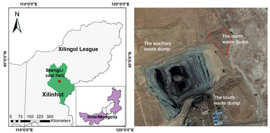
Figure 1.
Location of the ShengLi coal field and the North Waste Dump.
The North Waste Dump has a length of 1672 m and a width of 1155 m, with four berms. Each berm is nearly 15 m high and the slope angle is approximately 33°. The North Waste Dump was reclaimed from 2008 to 2011, with a green coverage of 101 ha. Due to the semi-arid grassland climate, the mining area experiences strong winds, and has plentiful sand, and large temperature differences. After the reclamation is finished, the manual environmental management stopped at 2013, resulting in the degradation of the vegetation. Moreover, soil erosion ditch and slope collapse were found in the field investigation, which caused great damage to the development of the mining area.
2.2. Image Collection and Field Survey
The flight platform selected in the study was the DJI Matrice100 (DJI Technology Co., Shenzhen, China), equipped with a matching digital camera of ZenmuseX3 (Figure 2; Table 1). The Matrice100 fuselage is made of carbon fiber material, making it flexible and light. It has a wheelbase of 650 mm, a horizontal hovering accuracy of 2.5 m, a vertical hovering accuracy of 0.5 m and a maximum wind speed tolerance of 10 m/s. It also has a maximum flight duration of 40 min. The UAS incorporates a digital camera ZenmuseX3 (DJI Technology Co., Shenzhen, China), which is automatically trigged by the Matrice100 (Figure 2; Table 1).
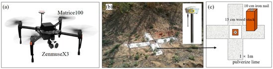
Figure 2.
Study equipment and materials. (a) Matrice100 and ZenmuseX3 camera, (b) ground control points (GCPs) were measured by Trimble R8 global navigation satellite system (GNSS), (c) detailed description of GCPs.

Table 1.
The specific parameters of the Matrice100 and ZenmuseX3 camera.
The flight was performed on 30 May 2017, the end of spring and early summer. The weather in the study area was always windy and cloudy with a prevailing west wind during this period. To minimize the influence of wind flow on the track, the flight route was situated along the east–west direction. The flight route was planned and processed automatically using the DJI GS Pro (DJI Technology Co., Shenzhen, China), an iPad App to conduct automated flight missions. The flight altitude was set to 115 m, and the photograph overlaps were 80 × 60% in the two dimensions. To overcome the influence of wind, the flight survey was processed at 6–9 a.m., and it took 57 minutes to capture a total of 815 photos. Our flight mission covered nearly 200 ha, which is slightly larger than the North Waste Dump of 105 ha.
Furthermore, 32 GCPs were designed on different berms and periphery of the waste dump. For a clearly identification of GCPs in georeferencing, the GCPs were designed with a cross shape of 1 × 1 m, using pulverized lime. A wood stack embedded with a 10 cm iron nail was placed in the center of the cross. The purpose of the nail was for more accurate positioning, while the wood stack was to ensure the stability when measuring on the ground (Figure 2). The approach to GCP design was low cost and good recognition, which has been used in our previous study [39]. The GNSS survey of each GCP was undertaken using a Trimble R8 GNSS (Trimble, USA) based on a position correction provided by continuously operating reference station (CORS) in the study area, which provided with a 2 cm accuracy. The coordinate system was Gauss-Kruger zone 20 with Beijing1954 projection system. Considering the time and efficiency, we chose to drive to deploy the GCPs in the study area.
2.3. Image Processing and Digital Surface Model (DSM) Generation
The processing of the aerial photos in this study was performed using the commercial software Pix4Dmapper (Pix4D, Switzerland). It allows a three-dimensional model to be reconstructed using SfM photogrammetry. The process is fully automatic, fast and highly accurate, which enables operators with no professional knowledge to quickly acquire accurate DSMs with minimal manual intervention. During the process, the software adjusts the interior and exterior camera orientation parameters to generate a three-dimensional point cloud based on the photo information. All of projects were processed under the same setting parameters in software (Table 2).
Table 2.
Setting parameters in Pix4Dmapper.
GCPs are usually used in a bundle block adjustment (BBA) process for precise positioning. Numerous studies proved that the number and distribution of GCPs can affect the final accuracy [26,32,37,38,40]. Given this, this study designed eight different GCP types to find the effective GCP configuration (Figure 3). Based on previous studies, GCPs placed on the edge of the study area could optimize the horizontal accuracy [26]. Besides, a uniform GCP distribution attained a better accuracy [26,41]. Therefore, the rules to place the GCPs were as follows:
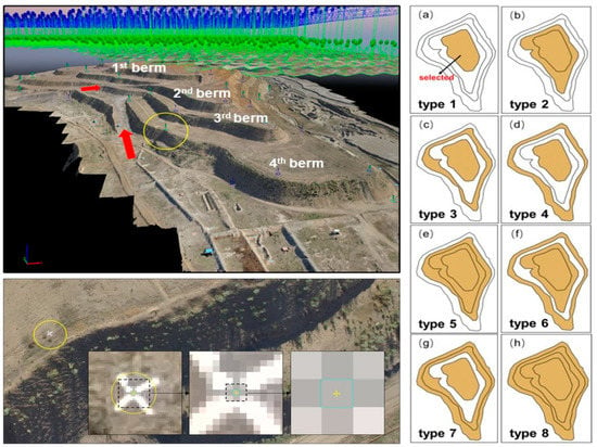
Figure 3.
Eight GCP configurations with 1–7 GCPs placed on each type: (a) 1st berm, (b) 1st and 2nd berms, (c) 1st and 3rd berms, (d) 1st and 4th berms, (e) 1st, 2nd, and 3rd berms, (f) 1st, 2nd, and 4th berms, (g) 1st, 3rd, and 4th berms, and (h) all four berms. The red arrow is our driving track in the field investigation.
- Four GCPs were designed on the periphery of the waste dump to reduce the edge deformation;
- The 1st berm was selected in all eight types of GCP configuration to ensure a reasonable spatial distribution, as shown below;
- Different numbers of GCPs (from one to seven) were designed in each selected berm of the eight types;
- The GCPs were located at the edge of each berm to ensure the horizontal accuracy.
Based on our rules, 56 (8 × 7) combinations were processed in this study. We made an electronic attachment to introduce the detailed GCPs combination of each project. During the process, the identification of GCPs is manually handled in the software. According to our design rules of GCPs (Figure 2c), the midpoint of the cross shape should be selected to identify as the GCP (Figure 3). Nevertheless, the identification process was an artificial operation, so the subjectivity was inevitable. To minimize this effect, the process was handled by author He Ren alone. Finally, the DSMs of 5.95 cm ground sample distance (GSD) were obtained. Due to the terrain elevation difference of the waste dump, the images of the project may not have the same GSD. In the study, the GSD was an average computed automatically by the software. According to the quality report generated from Pix4Dmapper software automatically, all projects met the accuracy requirements. During the initial processing, the relative difference of all projects was below 3% between the initial and optimized internal camera parameters and all 815 photos were calibrated. The georeferencing results of each project showed that the mean root mean square error (RMSE) values of the GCPs were almost always below the GSD values, with a range of 1.8–4.0 cm.
2.4. Accuracy Evaluation
The accuracy of all DSMs was evaluated using a total of 116 check points (CPs) measured like GCPs. Considering the special structure, the CPs were placed on both the berm and slope of the waste dump. A total of 79 CPs were designed on the berm with 37 CPs on the slope due to the measuring environment (Figure 4). The RMSE was used to verify the vertical accuracy of the DSM. To this end, the vertical coordinate of the CPs was extracted from the DSM using ArcGIS 10.2 and compared to the GNSS coordinate, resulting in the RMSEs, as follows:
where N is the number of CPs, ZCPs was the vertical coordinate of CPs measured in GNSS survey, and the ZDSM was the vertical coordinate of CPs extracted from the DSM.
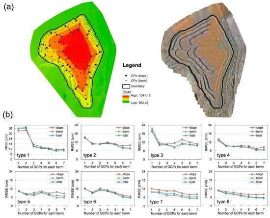
Figure 4.
Accuracy variations for different configuration types. (a) the DSM and the orthomosaic, (b) the root mean square errors (RMSEs) obtained for each type.
3. Results
3.1. Accuracy Comparison of Different Ground Control Point (GCP) Configurations
A total of 56 DSMs were obtained from the Pix4Dmapper (type 8-7 is shown in Figure 4). In this paper, type 8-7 signifies that seven GCPs were designed in each berm in type 8, and other types also follow this recording way. For each GCP configuration, we calculated three different RMSE of CPs from Equation (1), including the 79 CPs on the berm, 37 CPs on the slope and the total of 116 CPs. The total RMSE had a maximum and minimum of 36.61 and 5.59 cm, respectively, which corresponded to the type 1-2 and type 8-7. The same results were found in the RMSE of the berm, with a maximum and minimum of 34.12 and 4.45 cm, respectively. However, the RMSE of the slope was 37.73 and 6.81 cm, corresponding to the type 1-2 and type 6-7 respectively.
Moreover, a decreasing trend of all three kinds of RMSE was found when the number of GCPs increased from one to seven on each berm. Previous studies suggested that an increased number of GCPs improves the vertical accuracy of a DSM, which is also proved by our results. As the number of berms increased (equivalently to the increased number of GCPs), the RMSE showed a downwards trend. In the case of a single berm selected in the study (type 1), the total RMSE changed dramatically from 36.61 to 10.31 cm finally when the number of GCPs was increased from one to seven. Furthermore, the total RMSE was in the range of 7.21–0.16, 6.01–12.26, and 5.69–10.75 cm for two berms (types 2, 3, and 4), three berms (types 5, 6, and 7), and four berms (type 8), respectively. As the number of GCPs increased from 1 to 7 on each berm (Fig. 4(b)), we found that the RMSE change was more pronounced on the slope, while the change in the berm and total RMSE was more subdued. The RMSE of the slope was higher, but the overall trend was consistent with those of the berm and the total.
In order to better view the influence of the number of GCPs on the DSM accuracy for each type, we calculated the deviation of CPs in GSD units. We divided into five threshold standards (Figure 5), and computed the number of CPs under different standards on both slope and berm respectively. The proportion of different standards changes substantially with the increased number of berms (referred to as the increased number of GCPs; Figure 4). For the GCPs set on one berm, the deviation of types 1-1 and 1-2 were mostly greater than 4 GSD, while the proportion of CPs that was less than 2 GSD was below 25% (Figure 5a). However, the proportion of CPs less than 2 GSD improved to more than 50% as the number of GCPs increased. A similar situation was found for GCPs set on berms (types 2, 3 and 4). The proportion of less than 2 GSD increased from 40% to around 80% with the increased number of GCPs, except for a few special cases (types 2-4, 3-3, and 3-5). At the same time, the proportion of CPs greater than 3 GSD decreased. Of note, the proportion of CPs greater than 3 GSD was already less than 10% for type 4. For GCPs set on three berms (types 5, 6, and 7), the change between statistical standards became less clear, and the results had better overall accuracies. The proportion of CPs greater than 3 GSD was substantially reduced to 10%, with a marked reduction compared to the GCPs set on one and two berms. For GCPs set on four berms, the proportion of CPs whose deviation was greater than 3 GSD was further reduced, especially for the types 8-5 and 8-6. Based on our results, the proportion of CPs with a high deviation gradually decreased with the number of berms, and higher deviations (>4 GSD) gradually disappeared with more GCPs on each berm.
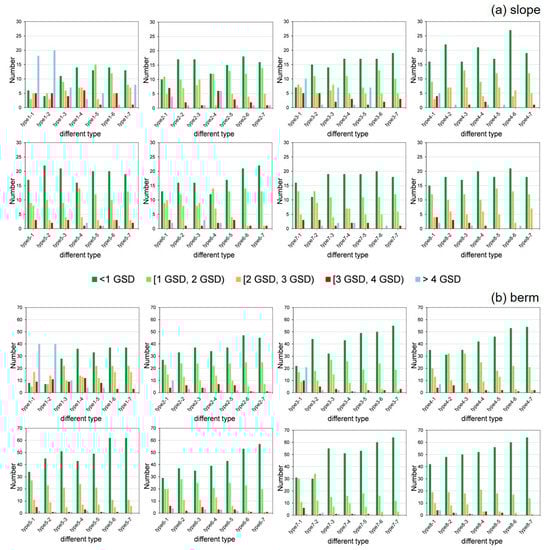
Figure 5.
Number of check points (CPs) under different statistical standards (units: GSD). (a) Slope, a total of 37 CPs, (b) berm, a total of 79 CPs.
These observations were verified and were more pronounced on the berm (Figure 5b). As the number of berms increased, the high-valued RMSE (>3 GSD) decreased, except for type 8-1. Furthermore, we found that the proportion of CPs greater than 3 GSD for each type was slightly lower than that of the slope, which is also consistent with the line results (Figure 4b).
3.2. Influence of the Total Number of GCPs on DSM Accuracy
The RMSE decreased with the number of berms (which indicates more GCPs; Figure 4). Furthermore, the same number of GCPs showed a deviation in the RMSE when laid on different numbers of berms (Figure 6). A worse accuracy occurred when the GCPs were laid on one berm (type 1). For n = 6, the RMSE of type 1-2 was 36.61 cm, which is much greater than type 2-1 at 15.16 cm, type 3-1 at 20.16 cm, and type 4-1 at 13.42 cm. For n = 7, the RMSE of type 1-3 was 15.54 cm, which is greater than those of type 5-1 at 10.34 cm, type 6-1 at 12.26 cm, and type 7-1 at 9.86 cm. However, deviations in the RMSE decreased as the number of GCPs increased. For n = 8, the RMSE of type 1-4 was still the highest, but the deviation reduced to 2.28–3.9 cm. This deviation was reduced to 0.21–0.32 cm for n = 10. When the number of berms increased from two (types 2, 3, and 4) to three (types 5, 6, and 7) or four (type 8), the RMSE did not significantly decrease, and a higher accuracy was achieved by setting the GCPs on two berms. The GCP configurations on three berms, in the case of n = 8, had a worse accuracy than on two berms (type 4-3) with a RMSE of 9.02 cm. For n = 16, all GCP configurations on two berms (types 2-6, 3-6, and 4-6) had a lower RMSE than three berms. Similarly, this occurred when the GCPs were laid on four berms. For n = 8, the RMSE of types 3-2 and 4-2 were 10.39 and 9.36 cm, respectively, but type 8-1 was 10.75 cm. For n = 12, the RMSE of type 3-4 was 8.99 cm, which was lower than type 8-2 at 9.04 cm. For n = 16, the RMSE of type 8-3 was 8.55 cm, which was higher than types 2-6 at 8.1 cm and 4-6 at 6.79 cm. From our results, considering the resources and efficiency (red arrow in Figure 3 was our track in the field investigation), the same number of GCPs on two berms was the most suitable way to control the accuracy compared to other types.
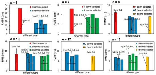
Figure 6.
RMSE deviation based on the same number of GCPs (red bar—type 1; blue bar—types 2, 3 and 4; green bar—types 5, 6, and 7; yellow bar—type 8).
The variation of total RMSE value with the total number of GCPs was shown in Figure 7. For a better visualization, the RMSEs over 30 cm are not shown. It should be pointed out that different types had different values in the case of the same number of GCPs (Figure 4), so three different RMSE standards, including maximum, minimum and mean values, were calculated. The results showed that the total RMSE of 116 CPs showed a decreasing trend with more GCPs. The RMSE decreased sharply from 36 cm to around 13 cm when the number of GCPs increased from 5 to 9 in the study area. Then, this decline became more gradual, with an RMSE of 9—13 cm as the number of GCPs increased to 19. Furthermore, the RMSE further reduced to less than 1GSD (< 6 cm) when the number of GCPs was increased to 32.
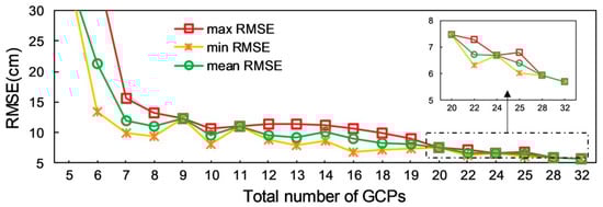
Figure 7.
RMSE of DSMs for different number of GCPs in the study area.
3.3. Comparison of Types 2,3 and 4 on DSM Accuracy
Three types of placing the GCPs on two berms were explored in the study, including type 2 (1st and 2nd berms), type 3 (1st and 3rd berms) and type 4 (1st and 4th berms; Figure 3). Based on the same number of selected berms and GCPs, the GCP configuration in type 4 had a higher precision with lower RMSEs compared with type 2 and type 3. The primary difference between these types was the spatial distribution due to the selected berms. The results in [10] suggested that the orthophoto accuracy is related to the increasing distance between GCPs in the study area. Also, [12] showed that the local accuracy of a DSM decreased by 9 cm when the distance to the closest GCP increased to 100 m.
In this section, we calculated the maximum distance of each GCP configuration (Appendix A). However, in this study, we set four GCPs on the periphery of the waste dump, and the maximum distance in all projects is 1629 m, the distance between the north and south points. The maximum distance calculated in this section is the distance between the GCPs placed on the berm, but not the GCPs outside the waste dump. The distance is calculated as follows:
where (, , ) and (, , ) represents the selected GCPs measured by GNSS RTK.
From the results (Figure 8), a high correlation was found between the maximum distance of GCPs and the RMSE of CPs. We calculated the Pearson correlation coefficient between maximum distance and total RMSE using SPSS software, with a Pearson’s r of 0.747** (significantly correlated at the 0.01 level, two-tailed). It also had a decreasing trend as the maximum distance increased at a rate of 0.64cm per 100 m. Our results also suggested that the type 4 (1st and 4th berms) was the best GCP configuration for DSM in construction in the study area when considering two berms.
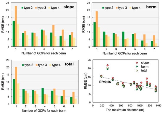
Figure 8.
Accuracy comparisons between types 2, 3, and 4.
3.4. Limitations and Discussion
A total of 32 GCPs were used in the 105 ha study area with a density of 0.3/ha, which is a relatively small number compared with previous studies [22,42,43,44,45]. In [27], the authors provided a good summary of the variable number of GCPs. However, a simple increase in the number of GCPs was inefficient and difficult in the waste dump, where the height difference between berms was large. As the goal of this work was to find the most effective type of GCP configuration with a set number of GCPs, a variable number of GCPs on each berm will be considered in future work. Besides, a total station should be considered to locate the GCPs when a small GSD of images was acquired [14,37,45]. The GSD of UAS products was 5.95 cm in this study, therefore both the CPs and GCPs measured by GNSS RTK can meet the need of accuracy verification.
The monitoring of slope deformation is a problem concerned with waste dumps, therefore the slope accuracy was also evaluated in this study. However, the horizontal accuracy of the waste dumps was not verified in this study. The horizontal accuracy can be optimized by placing GCPs at the edge of the study area [38], and thus we placed the GCPs at the edge of each berm in the survey to minimize the horizontal deformation. Even so, the error still existed (Table 3). We selected the GCPs not used in BBA as quality check points (QCPs) to verify the horizontal accuracy of DSMs. The coordinates of each QCP were identified in the orthomosaic images derived from UAS using ArcGIS 10. 2. The horizontal accuracy gradually approached one GSD as the number of GCPs increased. Since the berm of the dump site is flat, the horizontal displacement of nearly 1 GSD has little influence on the vertical accuracy of the CPs. However, considering the slope angle of the waste dump, the vertical deviation of CPs would be enlarged when the horizontal accuracy would suffer from a slight translation. Oblique images are proved to improve the camera calibration in the block, and are now being used to improve the reconstruction accuracy [27,37,46]. In [43], the best horizontal accuracy of a road cut-slope was achieved by the photogrammetric products derived from the combination of images obtained from different angles, which also has been proved in [27]. Manfreda et al. [27] suggested that the combination of different flights may be beneficial for DSM accuracy. They also argued that the use of the tilted camera can enhance the effective information of inclined surfaces and provide higher vertical accuracy of DSM.
Table 3.
The horizontal accuracy verification of DSMs of type 7 (unit: cm).
4. Conclusions
In this paper, we provided DSM constructions of a coal waste dumps using an unmanned aerial vehicle equipped with a consumer-grade digital camera. The vertical accuracy of DSMs generated from different GCP configurations was assessed using 116 CPs measured by GNSS RTK, which evenly located at the slope and berm of the waste dump. Our results suggested that the vertical accuracy of DSMs improved gradually as the number of GCPs increased from 5 to 32 and the total RMSE reduced from 36.6 to 5.3 cm. We also found that the same number of GCPs deployed on two berms (type 2, 3, and 4) had a better accuracy and efficiency compared to the other types. Moreover, there is still a difference in accuracy when choosing two different berms. The type 4 (1st and 4th berms) had better accuracy than type 2 (1st and 2nd berms) and type 3 (1st and 3rd berms). The statistical results showed that the total RMSE value of type 4 is smaller than that of type 2 and type 3, which are 0.12–6.74 cm (0.02–1.13 GSD) and 0.66–2.56 cm (0.11–0.43 GSD) respectively. Based on our research results, some suggestions are put forward for coal waste dumps in mining areas:
- (1)
- In the case of the same GCP numbers, setting GCPs on two berms is enough to limit the vertical accuracy of the DSM. Compared with setting GCPs on one berm, the accuracy substantially improved. Moreover, instead of setting on three or four berms, substantial human and material resources can be saved using two berms.
- (2)
- In coal waste dumps with four berms, the 1st (highest) and 4th (lowest) berms are the best GCP configuration for DSM construction to obtain higher vertical accuracy.
- (3)
- Our research result can be a reference for similar waste dumps with four berms and also engineering piles using multiple berms.
UAS is now popular in scientific research, but it is still a relatively ‘new technology’ in small mining areas. However, as the technology develops and matures, it will become widely used, which is similar to that of the GNSS technology which was first introduced in land surveying.
Author Contributions
Conceptualization, W.X. and Y.Z.; methodology, H.R.; software, H.R.; validation, H.R. and X.W.; formal analysis, T.S.; investigation, X.W. and T.S.; resources, W.X.; writing—original draft preparation, H.R.; writing—review and editing, W.X. and H.R.; visualization, H.R.; project administration, W.X.; funding acquisition, W.X. All authors have read and agreed to the published version of the manuscript.
Funding
This research was funded by the National Key R&D Program of China [grant No. 2016YFC0501103] the Open Fund of State Key Laboratory of Water Resource Protection and Utilization in Coal Mining [grant No. SHJT-16-30.16].
Acknowledgments
The authors wish to thank Jianyong Zhang, who gave us much valuable advice in the early stages of this work. Also, the authors thank Xin Wang and Tao Sui for their field survey.
Conflicts of Interest
The authors declare no conflict of interest. The funders had no role in the design of the study; in the collection, analyses, or interpretation of data; in the writing of the manuscript; or in the decision to publish the results.
Appendix A
| Project | Distance (m) | RMSE-Slope (cm) | RMSE-Berm (cm) | RMSE-Total (cm) |
| type 2-1 | 189.57 | 15.54 | 14.98 | 15.16 |
| type 2-2 | 545.67 | 21.61 | 19.57 | 20.16 |
| type 2-3 | 532.19 | 14.28 | 12.99 | 13.42 |
| type 2-4 | 882.03 | 10.58 | 11.17 | 10.98 |
| type 2-5 | 947.75 | 11.45 | 9.86 | 10.39 |
| type 2-6 | 947.75 | 9.69 | 9.21 | 9.36 |
| type 2-7 | 1029.69 | 10.77 | 10.57 | 10.64 |
| type 3-1 | 321.88 | 10.65 | 10.25 | 10.38 |
| type 3-2 | 644.98 | 9.14 | 9.1419 | 9.02 |
| type 3-3 | 817.65 | 11.92 | 11.20 | 11.44 |
| type 3-4 | 1042.03 | 11.57 | 8.13 | 8.99 |
| type 3-5 | 1159.43 | 9.62 | 8.49 | 8.87 |
| type 3-6 | 1159.43 | 10.73 | 10.26 | 10.41 |
| type 3-7 | 1159.43 | 13.89 | 10.49 | 11.24 |
| type 4-1 | 428.14 | 9.29 | 8.24 | 8.59 |
| type 4-2 | 665.96 | 9.40 | 7.55 | 8.18 |
| type 4-3 | 1002.2 | 11.98 | 10.08 | 10.65 |
| type 4-4 | 1002.2 | 7.48 | 6.44 | 6.79 |
| type 4-5 | 1347.25 | 9.82 | 7.35 | 7.87 |
| type 4-6 | 1347.25 | 10.89 | 9.69 | 9.99 |
| type 4-7 | 1347.25 | 8.64 | 6.43 | 7.21 |
References
- Xiao, W.; Hu, Z.; Fu, Y. Zoning of land reclamation in coal mining area and new progresses for the past 10 years. Int. J. Coal. Sci. Technol. 2014, 1, 177–183. [Google Scholar] [CrossRef]
- Cheng, L.; Skousen, J.G. Comparison of international mine reclamation bonding systems with recommendations for China. Int. J. Coal. Sci. Technol. 2017, 4, 67–79. [Google Scholar] [CrossRef]
- Chugh, Y.P. Concurrent mining and reclamation for underground coal mining subsidence impacts in China. Int. J. Coal. Sci. Technol. 2018, 5, 18–35. [Google Scholar] [CrossRef]
- Wang, J.; Wang, H.; Cao, Y.; Bai, Z.; Qin, Q. Effects of soil and topographic factors on vegetation restoration in opencast coal mine dumps located in a loess area. Sci. Rep. 2016, 6, 1–11. [Google Scholar] [CrossRef] [PubMed]
- Lv, X.; Xiao, W.; Zhao, Y.; Zhang, W.; Li, S.; Sun, H. Drivers of spatio-temporal ecological vulnerability in an arid, coal mining region in Western China. Ecol. Indic. 2019, 106, 105475. [Google Scholar] [CrossRef]
- Xiao, W.; Lv, X.; Zhao, Y.; Sun, H.; Li, J. Ecological resilience assessment of an arid coal mining area using index of entropy and linear weighted analysis: A case study of Shendong Coalfield, China. Ecol. Indic. 2020, 109, 105843. [Google Scholar] [CrossRef]
- Szostak, M.; Knapik, K.; Wężyk, P.; Likus-Cieślik, J.; Pietrzykowski, M. Fusing Sentinel-2 Imagery and ALS Point Clouds for Defining LULC Changes on Reclaimed Areas by Afforestation. Sustainability 2019, 11, 1251. [Google Scholar] [CrossRef]
- Yellishetty, M.; Darlington, W.J. Effects of monsoonal rainfall on waste dump stability and respective geo-environmental issues: A case study. Environ. Earth. Sci. 2011, 63, 1169–1177. [Google Scholar] [CrossRef]
- Cho, Y.C.; Song, Y.S. Deformation measurements and a stability analysis of the slope at a coal mine waste dump. Ecol. Eng. 2014, 68, 189–199. [Google Scholar] [CrossRef]
- Gong, C.; Lei, S.; Bian, Z.; Liu, Y.; Zhang, Z.; Cheng, W. Analysis of the Development of an Erosion Gully in an Open-Pit Coal Mine Dump During a Winter Freeze-Thaw Cycle by Using Low-Cost UAVs. Remote. Sens. 2019, 11, 1356. [Google Scholar] [CrossRef]
- Zhang, L.; Wang, J.; Bai, Z.; Lv, C. Effects of vegetation on runoff and soil erosion on reclaimed land in an opencast coal-mine dump in a loess area. Catena 2015, 128, 44–53. [Google Scholar] [CrossRef]
- Meinen, B.U.; Robinson, D.T. Streambank topography: An accuracy assessment of UAV-based and traditional 3D reconstructions. Int. J. Remote. Sens. 2020, 41, 1–18. [Google Scholar] [CrossRef]
- Cardenal, J.; Fernández, T.; Pérez-García, J.L.; Gómez-López, J.M. Measurement of road surface deformation using images captured from UAVs. Remote. Sens. 2019, 11, 1507. [Google Scholar] [CrossRef]
- Bolkas, D. Assessment of GCP Number and Separation Distance for Small UAS Surveys with and without GNSS-PPK Positioning. J. Surv. Eng. 2019, 145, 04019007. [Google Scholar] [CrossRef]
- Cook, K.L. An evaluation of the effectiveness of low-cost UAVs and structure from motion for geomorphic change detection. Geomorphology 2017, 278, 195–208. [Google Scholar] [CrossRef]
- Gillan, J.K.; Karl, J.W.; Elaksher, A.; Duniway, M.C. Fine-resolution repeat topographic surveying of dryland landscapes using UAS-based structure-from-motion photogrammetry: Assessing accuracy and precision against traditional ground-based erosion measurements. Remote. Sens. 2017, 9, 437. [Google Scholar] [CrossRef]
- Deng, L.; Mao, Z.; Li, X.; Hu, Z.; Duan, F.; Yan, Y. UAV-based multispectral remote sensing for precision agriculture: A comparison between different cameras. ISPRS J. Photogram. Remote. Sens. 2018, 146, 124–136. [Google Scholar] [CrossRef]
- Bendig, J.; Bolten, A.; Bennertz, S.; Broscheit, J.; Eichfuss, S.; Bareth, G. Estimating biomass of barley using crop surface models (CSMs) derived from UAV-based RGB imaging. Remote. Sens. 2014, 6, 10395–10412. [Google Scholar] [CrossRef]
- Bendig, J.; Yu, K.; Aasen, H.; Bolten, A.; Bennertz, S.; Broscheit, J.; Bareth, G. Combining UAV-based plant height from crop surface models, visible, and near infrared vegetation indices for biomass monitoring in barley. Int. J. Appl. Earth. Obs. 2015, 39, 79–87. [Google Scholar] [CrossRef]
- Tomaštík, J.; Mokroš, M.; Saloň, Š.; Chudý, F.; Tunák, D. Accuracy of photogrammetric UAV-based point clouds under conditions of partially-open forest canopy. Forests 2017, 8, 151. [Google Scholar] [CrossRef]
- Kršák, B.; Blišťan, P.; Pauliková, A.; Puškárová, P.; Kovanič, Ľ.; Palková, J.; Zelizňaková, V. Use of low-cost UAV photogrammetry to analyze the accuracy of a digital elevation model in a case study. Measurement 2016, 91, 276–287. [Google Scholar] [CrossRef]
- Messinger, M.; Silman, M. Unmanned aerial vehicles for the assessment and monitoring of environmental contamination: An example from coal ash spills. Environ. Pollut. 2016, 218, 889–894. [Google Scholar] [CrossRef]
- Johansen, K.; Erskine, P.D.; McCabe, M.F. Using Unmanned Aerial Vehicles to assess the rehabilitation performance of open cut coal mines. J. Clean. Prod. 2019, 209, 819–833. [Google Scholar] [CrossRef]
- Ren, H.; Zhao, Y.; Xiao, W.; Hu, Z. A review of UAV monitoring in mining areas: Current status and future perspectives. Int. J. Coal. Sci. Technol. 2019, 1–14. [Google Scholar] [CrossRef]
- Casella, V.; Chiabrando, F.; Franzini, M.; Manzino, A.M. Accuracy Assessment of A UAV Block by Different Software Packages, Processing Schemes and Validation Strategies. ISPRS Int. J. Geo-Inf. 2020, 9, 164. [Google Scholar] [CrossRef]
- Clapuyt, F.; Vanacker, V.; Van Oost, K. Reproducibility of UAV-based earth topography reconstructions based on Structure-from-Motion algorithms. Geomorphology 2016, 260, 4–15. [Google Scholar] [CrossRef]
- Manfreda, S.; Dvorak, P.; Mullerova, J.; Herban, S.; Vuono, P.; Arranz Justel, J.J.; Perks, M. Assessing the Accuracy of Digital Surface Models Derived from Optical Imagery Acquired with Unmanned Aerial Systems. Drones 2019, 3, 15. [Google Scholar] [CrossRef]
- Benassi, F.; Dall’Asta, E.; Diotri, F.; Forlani, G.; Morra di Cella, U.; Roncella, R.; Santise, M. Testing accuracy and repeatability of UAV blocks oriented with GNSS-supported aerial triangulation. Remote. Sens. 2017, 9, 172. [Google Scholar] [CrossRef]
- James, M.R.; Robson, S. Mitigating systematic error in topographic models derived from UAV and ground-based image networks. Earth. Surf. Process Land. 2014, 39, 1413–1420. [Google Scholar] [CrossRef]
- Shahbazi, M.; Sohn, G.; Théau, J.; Menard, P. Development and evaluation of a UAV-photogrammetry system for precise 3D environmental modeling. Sensors 2015, 15, 27493–27524. [Google Scholar] [CrossRef]
- Oniga, V.E.; Pfeifer, N.; Loghin, A.M. 3D calibration test-field for digital cameras mounted on unmanned aerial systems (UAS). Remote. Sens. 2018, 10, 2017. [Google Scholar] [CrossRef]
- Uysal, M.; Toprak, A.S.; Polat, N. DEM generation with UAV Photogrammetry and accuracy analysis in Sahitler hill. Measurement 2015, 73, 539–543. [Google Scholar] [CrossRef]
- Martínez-Carricondo, P.; Agüera-Vega, F.; Carvajal-Ramírez, F.; Mesas-Carrascosa, F.J.; García-Ferrer, A.; Pérez-Porras, F.J. Assessment of UAV-photogrammetric mapping accuracy based on variation of ground control points. Int. J. Appl. Earth. Obs. Geoinf. 2018, 72, 1–10. [Google Scholar] [CrossRef]
- Gindraux, S.; Boesch, R.; Farinotti, D. Accuracy assessment of digital surface models from unmanned aerial vehicles’ imagery on glaciers. Remote. Sens. 2017, 9, 186. [Google Scholar] [CrossRef]
- Tahar, K.N. An evaluation on different number of ground control points in unmanned aerial vehicle photogrammetric block. Int. Arch. Photogramm. Remote Sens. Spat. Inf. Sci 2013, 40, 93–98. [Google Scholar] [CrossRef]
- Rangel, J.M.G.; Gonçalves, G.R.; Pérez, J.A. The impact of number and spatial distribution of GCPs on the positional accuracy of geospatial products derived from low-cost UASs. Int. J. Remote. Sens. 2018, 39, 7154–7171. [Google Scholar] [CrossRef]
- Forlani, G.; Diotri, F.; Cella, U.M.D.; Roncella, R. Indirect UAV strip georeferencing by on-board GNSS data under poor satellite coverage. Remote. Sens. 2019, 11, 1765. [Google Scholar] [CrossRef]
- Agüera-Vega, F.; Carvajal-Ramírez, F.; Martínez-Carricondo, P. Assessment of photogrammetric mapping accuracy based on variation ground control points number using unmanned aerial vehicle. Measurement 2017, 98, 221–227. [Google Scholar] [CrossRef]
- Ren, H.; Xiao, W.; Zhao, Y.; Hu, Z. Land damage assessment using maize aboveground biomass estimated from unmanned aerial vehicle in high groundwater level regions affected by underground coal mining. Environ. Sci. Pollut. R 2020. [Google Scholar] [CrossRef]
- Tomaštík, J.; Mokroš, M.; Surový, P.; Grznárová, A.; Merganič, J. UAV RTK/PPK Method—An Optimal Solution for Mapping Inaccessible Forested Areas? Remote. Sens. 2019, 11, 721. [Google Scholar] [CrossRef]
- Villanueva, J.K.S.; Blanco, A.C. Optimization of ground control point (GCP) configuration for unmanned aerial vehicle (UAV) survey using structure from motion (SfM). Int. Arch. Photogramm. Remote Sens. Spat. Inf. Sci. 2019, XLII-4/W12, 167–174. [Google Scholar] [CrossRef]
- James, M.R.; Robson, S.; d’Oleire-Oltmanns, S.; Niethammer, U. Optimising UAV topographic surveys processed with structure-from-motion: Ground control quality, quantity and bundle adjustment. Geomorphology 2017, 280, 51–66. [Google Scholar] [CrossRef]
- Agüera-Vega, F.; Carvajal-Ramírez, F.; Martínez-Carricondo, P.; López, J.S.H.; Mesas-Carrascosa, F.J.; García-Ferrer, A.; Pérez-Porras, F.J. Reconstruction of extreme topography from UAV structure from motion photogrammetry. Measurement 2018, 121, 127–138. [Google Scholar] [CrossRef]
- Oniga, V.E.; Breaban, A.I.; Pfeifer, N.; Chirila, C. Determining the Suitable Number of Ground Control Points for UAS Images Georeferencing by Varying Number and Spatial Distribution. Remote. Sens. 2020, 12, 876. [Google Scholar] [CrossRef]
- Harwin, S.; Lucieer, A.; Osborn, J. The Impact of the Calibration Method on the Accuracy of Point Clouds Derived Using Unmanned Aerial Vehicle Multi-View Stereopsis. Remote. Sens. 2015, 7, 11933–11953. [Google Scholar] [CrossRef]
- Zhou, Y.; Rupnik, E.; Faure, P.H.; Pierrot-Deseilligny, M. GNSS-assisted integrated sensor orientation with sensor pre-calibration for accurate corridor mapping. Sensors 2018, 18, 2783. [Google Scholar] [CrossRef]
© 2020 by the authors. Licensee MDPI, Basel, Switzerland. This article is an open access article distributed under the terms and conditions of the Creative Commons Attribution (CC BY) license (http://creativecommons.org/licenses/by/4.0/).