Article

Automated Georectification and Mosaicking of UAV-Based Hyperspectral Imagery from Push-Broom Sensors

1
Hydrology, Agriculture and Land Observation Group (HALO), Division of Biological and Environmental Science and Engineering, King Abdullah University of Science and Technology, Thuwal 23955-6900, Saudi Arabia
2
Discipline of Geography and Spatial Sciences, College of Sciences and Engineering, University of Tasmania, Hobart 7001, Australia
3
Center for Remote Sensing Applications (CRSA), Mohammed VI Polytechnic University, Ben Guerir 43150, Morocco
*
Author to whom correspondence should be addressed.
Remote Sens. 2020, 12(1), 34; https://doi.org/10.3390/rs12010034
Submission received: 27 October 2019 / Revised: 26 November 2019 / Accepted: 30 November 2019 / Published: 20 December 2019

Abstract

:
Hyperspectral systems integrated on unmanned aerial vehicles (UAV) provide unique opportunities to conduct high-resolution multitemporal spectral analysis for diverse applications. However, additional time-consuming rectification efforts in postprocessing are routinely required, since geometric distortions can be introduced due to UAV movements during flight, even if navigation/motion sensors are used to track the position of each scan. Part of the challenge in obtaining high-quality imagery relates to the lack of a fast processing workflow that can retrieve geometrically accurate mosaics while optimizing the ground data collection efforts. To address this problem, we explored a computationally robust automated georectification and mosaicking methodology. It operates effectively in a parallel computing environment and evaluates results against a number of high-spatial-resolution datasets (mm to cm resolution) collected using a push-broom sensor and an associated RGB frame-based camera. The methodology estimates the luminance of the hyperspectral swaths and coregisters these against a luminance RGB-based orthophoto. The procedure includes an improved coregistration strategy by integrating the Speeded-Up Robust Features (SURF) algorithm, with the Maximum Likelihood Estimator Sample Consensus (MLESAC) approach. SURF identifies common features between each swath and the RGB-orthomosaic, while MLESAC fits the best geometric transformation model to the retrieved matches. Individual scanlines are then geometrically transformed and merged into a single spatially continuous mosaic reaching high positional accuracies only with a few number of ground control points (GCPs). The capacity of the workflow to achieve high spatial accuracy was demonstrated by examining statistical metrics such as RMSE, MAE, and the relative positional accuracy at 95% confidence level. Comparison against a user-generated georectification demonstrates that the automated approach speeds up the coregistration process by 85%.

1. Introduction

Remote sensing has provided incredible advances in our capacity to observe and understand the earth system [1], with new and emerging technologies providing further opportunities for insights and understanding [2]. One of the key constraints in our observation capacity relates to the compromise between spatial and temporal resolution, i.e., space-based platforms tend to suffer from either spatial or temporal restrictions that affect the frequency and fidelity of retrievals. Within the last decade, developments in remote sensing using unmanned aerial vehicles (UAV) have provided a sensor-flexible platform that has lowered operational costs, while providing unprecedented spatial (<10 cm) and on-demand temporal resolution [3,4]. To leverage these technological advances, hyperspectral camera systems capturing radiances across the visible and near-infrared portions of the spectrum [5] have been developed, with diverse applications being presented in agriculture [6,7,8], forestry [9], and mining [10] studies. However, while UAV technology has progressed rapidly and there is a level of maturity in many sensing capabilities [11], routine application of hyperspectral imaging systems remains challenging and has been constrained by a lack of automation and processing options to streamline the image analysis. In particular, additional efforts are required in the integration of accurate positional sensors with spectral devices during image collection and subsequent automated geometric calibration frameworks based on image coregistration and ground control points. To realize this potential, UAV-based hyperspectral sensing systems need to provide radiometrically and geometrically accurate data that allow posterior quantitative analysis to be performed with confidence.
UAV-based image products are generally produced by stitching together hundreds of overlapping scanlines or frames captured on the fly [10]. However, when “matching” any two images, the transformation and reprojection undertaken by the fitting algorithms routinely introduce localized distortions. While the positional accuracy of an individual image may be on the order of a few centimeters, the accuracy of the completed mosaic may increase to the decimeter range as the positional errors accumulate through the merging process. In the case of scanning systems, image distortion can also result due to geometric noise induced by UAV movements. Likewise, accurately overlapping swaths requires a good number of matching and ground control points (GCPs) to avoid further distortion in the final mosaic [11]. A range of hyperspectral sensor configurations is available for UAV-based integration, including point [12] and push-broom spectrometers, as well as 2D spectral imagers [3]. In general, the traditional image georectification process for any such system relies on positional, orientation, rotation, and acceleration data collected by Global Navigation Satellite Systems (GNSS) and/or Inertial Navigation Systems (INS) [13]. In the case of point spectrometers [12,14,15,16,17], spectra are collected with no integrated spatial reference, requiring ancillary data (onboard and in situ) to georeference the imagery. Push-broom sensors [18,19,20,21,22,23,24,25,26,27] offer a high spectral and spatial resolution by sampling individual lines of spectra during flight. However, the spatial accuracy of each scanline is highly dependent on flying conditions, with the resulting error constrained by GNSS/INS sensors accuracy [28] and the stability provided by the gimbal setup. Conversely, 2D cameras collect band sequential spectra data in two spatial dimensions or by integrating multiple synchronized cameras [29,30,31,32,33]. Such is the case of snapshot systems [34,35,36], which record all the bands simultaneously, with the advantage of capturing spatial and spectral data with every scene. In both cases, the mosaicking process of UAV-based spectral imaging requires rectification approaches [37,38], which, when integrated with an optimal combination of complementary sensors, assure the spatial accuracy of the products.
Multiple applications using UAV-based hyperspectral systems have been proposed in the literature, exploring a range of prototypes and georectification methods. For instance, Zarco-Tejada et al. [18,20] investigated the early detection of plant diseases and the seasonal trends of narrow-band physiological and structural vegetation indices using a Headwall micro-Hyperspec [21] VNIR push-broom sensor onboard a fixed-wing platform. In their studies, the geometric rectification of the 30 cm [18] and 40 cm [20] pixel resolution imagery was conducted using the PARGE [39] software, which relies on GNSS/INS parameters and a digital elevation model (DEM) to perform the ortho-rectification of airborne optical scanner imagery. Lucieer et al. [22], Turner et al. [23], and Malenovsky et al. [24], used the same sensor mounted on a multirotor aircraft, collecting 2–4 cm ground sample distance (GSD) hypercubes to map the health and status of vegetation. In these cases, the geometrical rectification was based on a dense network of ground control points in addition to using PARGE [39] and achieved a root mean square error (RMSE) of around 5 cm. A different arrangement was employed by Sankey et al., 2017, who collected 12 cm pixel resolution data by integrating the Headwall Nano-Hyperspec [21], and a Light Detection and Ranging (LiDAR) system onboard an octocopter for forest monitoring. Sankey et al. preprocessed the individual hyperspectral tiles in the SpectralView software [40], and then manually tied the georectified swaths to produce a single mosaic, achieving an RMSE of 0.94 m and 1.1 m in the X and Y dimensions, respectively. Recently, a boresight calibration of GNSS/INS has been explored by Habib et al. [41], in an attempt to directly derive the scanner position and orientation by defining the optimal/minimal flight and control/tie point configuration.
With an aim of reducing the required ground sampling efforts and the payload onboard, some studies have explored photogrammetry-based computer vision approaches to determine sensor orientations. Suomalainen et al. [26] and Turner et al. [23] developed processing workflows that include RGB frame-based scenes captured simultaneously with the hyperspectral imagery, to produce a DSM by using Structure from Motion (SfM) algorithms, and then feeding PARGE [39] with this high-resolution model, with resulting imagery achieving accuracies below 10 cm RMSE. Ramirez-Paredes et al. [37] sought to exploit the homographies between RGB frames to align line-to-line the hyperspectral data in the frame camera image plane, by using a low-cost payload on a radio-controlled airplane. Habib et al. [38] proposed an alternative mosaicking approach relying on image coregistration algorithms to stitch together hyperspectral swaths, which were previously rectified by feeding SpectralView [40] with a base-frame DSM, reaching submetric accuracies. Further, computer vision coregistration approaches have even been explored as standard video stabilization techniques [42,43,44] by performing a robust feature detection using Scale-invariant Feature Transform (SIFT), Speeded Up Robust Features (SURF), Features from Accelerated Segment Test (FAST), and Binary Robust Independent Elementary Features (BRIEF) key points between adjacent frames, then smoothing the sensor path and finally rendering the stabilized frames of a video.
From the approaches presented above, the semiautomated [18,20,22,26,39] solutions require additional efforts, including collection of a high number of GCPs and manually detecting matching points to produce decimeter accurate georectified mosaics. In contrast, previous semiautomated [37,38] methods identify pairs of points based on image coregistration algorithms, with the limitations involving manually identifying geometrical features [28], being compute-intense, and not exceeding the accuracies achieved by manually-based approaches. In general, all of the described techniques highlight the necessity for further research towards highly accurate, fast and fully automated methods that provide a balance between sensors payload, ancillary field data needs, and computational efficiency. An additional challenge is the massive volume of UAV-based hyperspectral data cubes (on the order of terabytes) that are now being collected [45], particularly for those studies where millimeter scales may be required (i.e., phenotyping investigations) [46]. All of these factors highlight the need for speeding up geo-processing to achieve highly accurate hyperspectral imagery while optimizing the data collection demands.
In view of the above, the goal of this research was to conduct a fully automated workflow to produce highly accurate georectified UAV-based hyperspectral mosaics collected by push-broom scanners and to optimize the geoprocessing time by adopting an efficient computing coregistration strategy, requiring a small number of GCPs. UAV-based hyperspectral scans and RGB scenes from two different experiments were used to assess the applicability of the proposed workflow, which follows the five stages of image coregistration process between individual hyperspectral scans and an RGB frame-based orthophoto [47], including: (i) feature detection and description, (ii) feature matching, (iii) inlier selection, (iv) derivation of a transformation function, and (v) image mosaicking. RGB frame-based orthophotos were used as a reference to georectify preprocessed hyperspectral swaths by implementing a parallelized routine of feature detector functions that find the corresponding points between them. The Speeded Up Robust Features (SURF) [48] matching algorithm was integrated with the Maximum Likelihood Estimation SAmple and Consensus (MLSAC) [49], estimator method to automate the coregistration processing. Accordingly, individual geographical transformations per swath were estimated, and the georectified strips were mosaicked. The computational robustness of the approach was evaluated by timing each step-process, and the spatial accuracy was assessed by determining standard accuracy metrics such as root mean square error (RMSE), mean absolute error (MAE), with the relative positional accuracy determined at the 95% confidence level. The proposed methodology provides a novel solution to expedite one of the most costly postprocessing stages of UAV-based hyperspectral remote sensing for push-broom sensors, implementing a simplified coregistration strategy and achieving high positional accurate results.

2. Materials and Methods

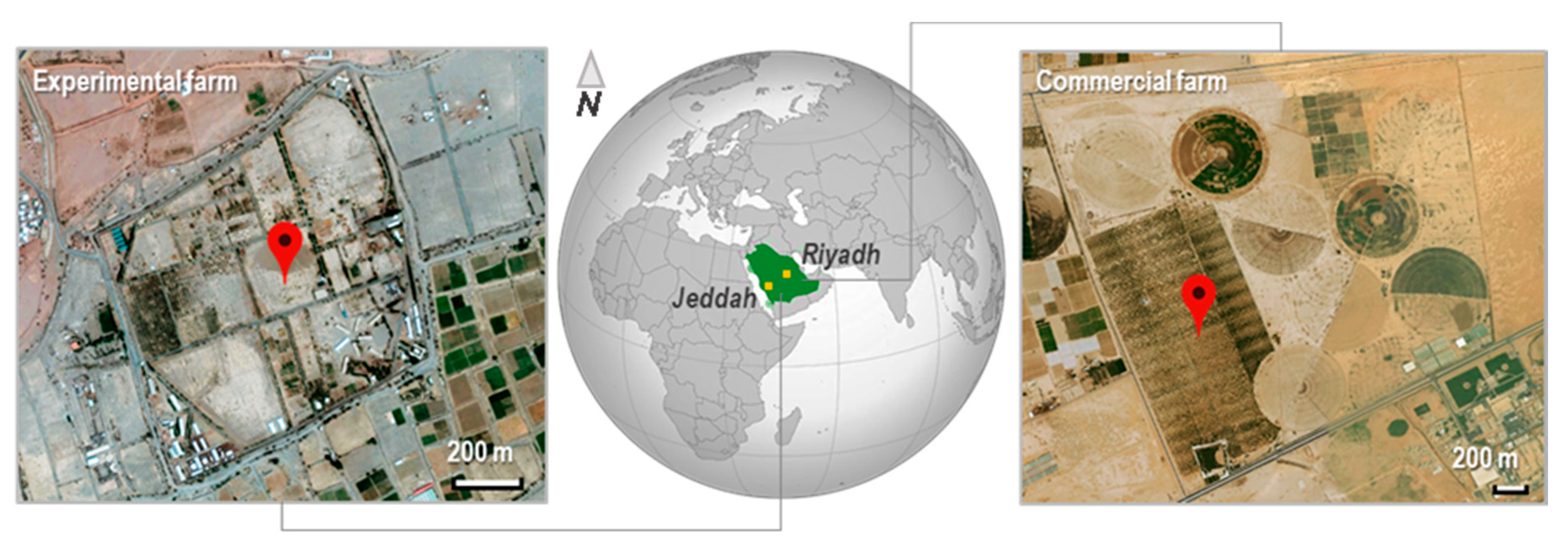
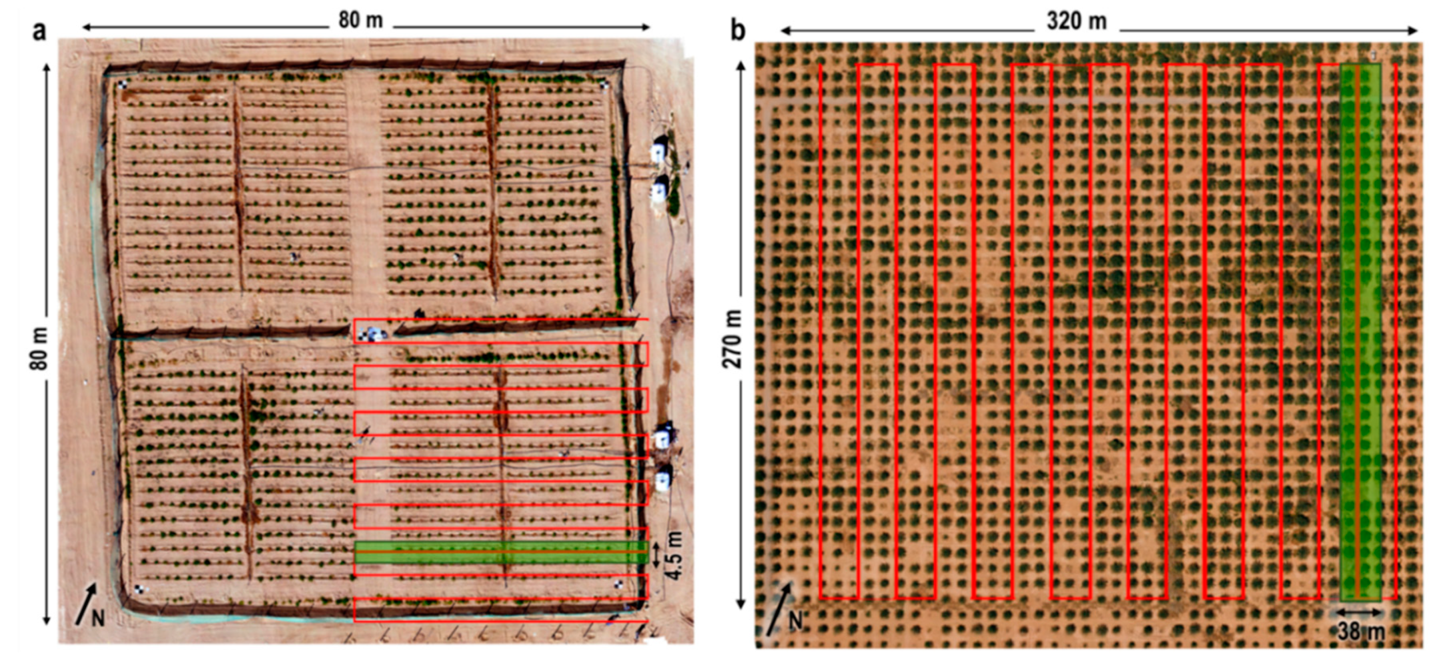
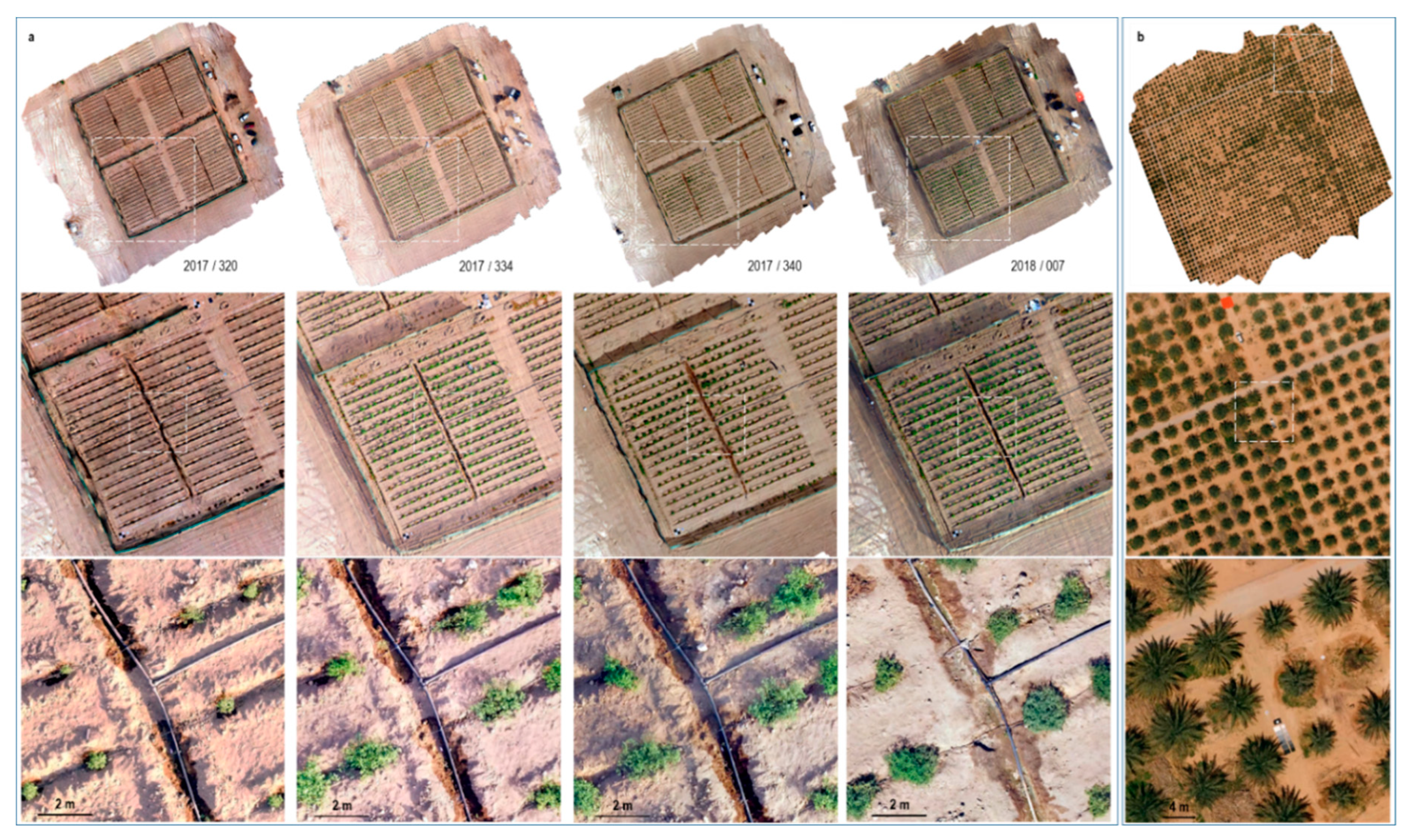
2.1. Study Area and Experimental Design

Data were collected from two experimental facilities in Saudi Arabia (Figure 1). The first dataset supports a phenotyping study undertaken over a wild tomato crop at the King Abdulaziz University experimental farm, located at Hada Al-Sham, approximately 60 km east of Jeddah [50]. The site is characterized by a tropical arid climate [49] with an annual rainfall below 100 mm and is situated in a valley at an elevation of approximately 250 m above sea-level, with a predominantly sandy loam soil type. Four campaigns were conducted during the winter season from November 2017 to the end of January 2018, when the average air temperature (during UAV flight) was between 10 and 35 °C. The second study site was a commercial date palm plantation near Al-Kharj [51], a city approximately 200 km southeast of Riyadh. The site is located in a desert depression approximately 1300 m above sea level, it has an average annual rainfall of 51 mm and has sandy desert soils that are irrigated by a natural spring [52]. A single campaign was undertaken during May 2018, when average daytime temperatures reached highs of around 33 °C. Both sites present quite different crop types and geographic extents, which allows an assessment of the transferability of the proposed georectification approach. For instance, a square area of 80 m × 80 m was established for the tomato experiment, comprising four fields with rows aligned along the north-east direction at approximately 2 m spacing. For the date plantation, a total area of approximately 8.7 hectares (270 m × 320 m) was overflown following a north-east direction, with a total of 1300 individual palms (equally spaced at 8 m intervals) captured.

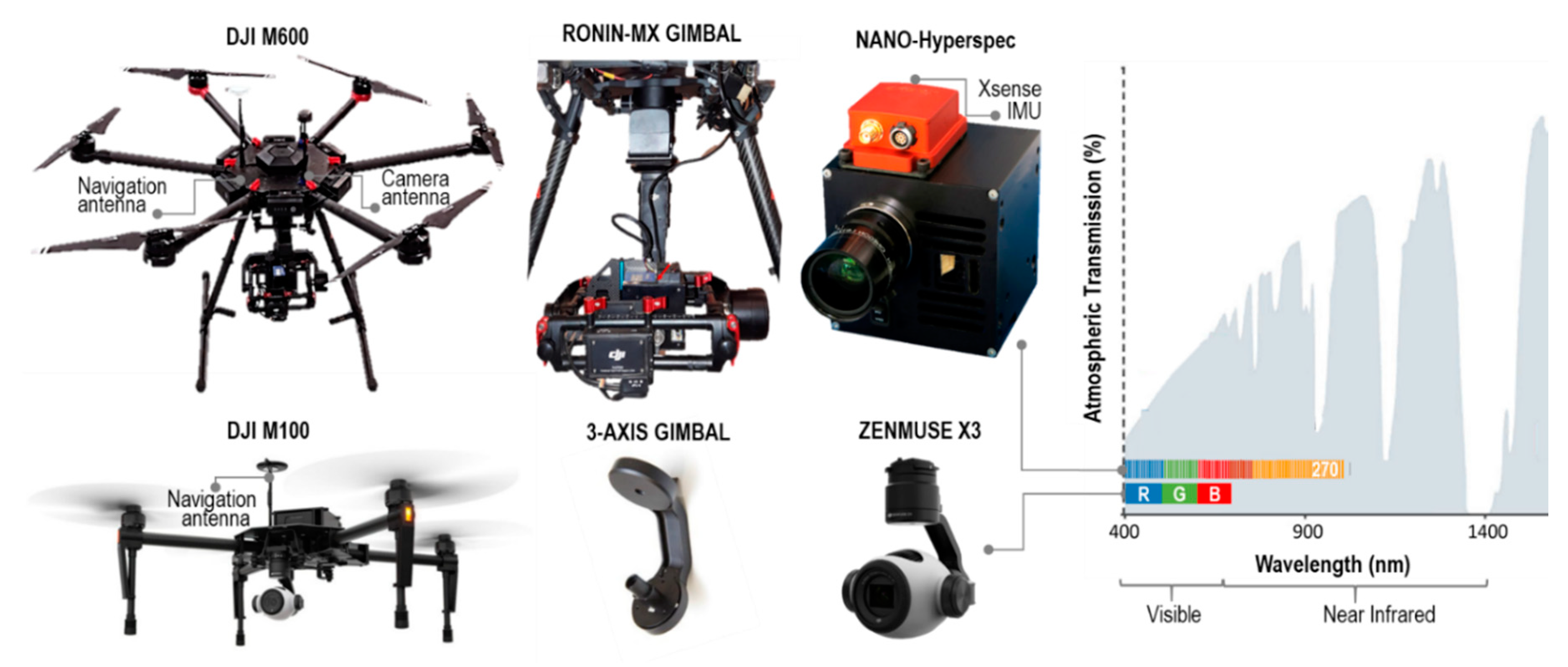
2.2. Unmanned Aerial Vehicles and Sensor Package

Two separate UAV-based remote sensing systems were used for data collection (Figure 2). Hyperspectral imagery was collected using a DJI Matrice 600 (M600) hexacopter [53] coupled with a Ronin-MX gimbal to reduce flight dynamic effects. The flight platform housed a Headwall Nano-Hyperspec [21] push-broom camera, with 12 mm lens and a horizontal field of view (FOV) of 21.1°, which gathered radiometric data in the 400–1000 nm range across 272 continuous bands and with 6 nm FWHM. Two GNSS antennas were mounted on the upper plate of the UAV, with one for the aircraft navigation and another for the hyperspectral camera. An Xsens inertial measurement unit (IMU) was paired with the camera and the GNSS antenna, to monitor the roll, pitch, and yaw motions. The total payload of the M600 was 3.65 kg, which constrains the flight time to approximately 20 min. Ancillary RGB imagery was captured using a DJI Matrice 100 (M100) quadcopter [54], which is paired with a 3-axis gimbal to keep the camera steady in the air, an IMU built in the main controller, and a single GNSS navigation antenna. An on-board Exmor CMOS Zenmuse X3 frame camera [55], with 20 mm optical lens and diagonal FOV of 94°, collected RGB data across a single spectral range (400–700 nm). The total payload of the M100 was 0.25 kg, constraining the flight time to approximately 20 min.

2.3. Flight Planning

Prior to each field campaign, a flight plan was designed depending on flight altitude, spatial resolution requirement, area to cover, overlap percentage between swaths, and lighting conditions (Figure 3). Additional preflight aspects to consider included planning for optimal atmospherical conditions. Morning hours close to solar noon under clear sky were preferred to avoid wind and thermals generated by environmental heating. The Universal Ground Control Station [56] desktop application was used to construct all UAV flight plans. For the tomatoes experiment, the hyperspectral swaths were collected using the M600, with 30% sidelap at a speed of 1 m/s and a height of 16 m, scanning at a frame rate of 100 fps to ensure square pixels. A total of four flights per campaign were required to collect 56 swaths, with a ground sampling distance (GSD) of 0.007 m. RGB data was captured with a 78% along-track overlap and 82% sidelap at a speed of 2 m/s and a height of 13 m, with a frame frequency of 0.33 fps. A total of 196 frames with a 0.005 m pixel size fully covered the area. For the date palms plantation, a total of 16 hyperspectral strips were scanned, reaching a GSD of 0.06 m with 40% sidelap, flying at a speed of 5 m/s and a height of 80 m above the ground, scanning at a frame rate of 100 fps. In addition, 184 RGB frames at a 0.04 m spatial resolution were captured with the M100, with an 82% along-track overlap and 87% sidelap, flying at a speed of 5 m/s and a height of 80 m. More detailed information on the specific flight configurations is provided in Table 1.

2.4. Ground Data Collection
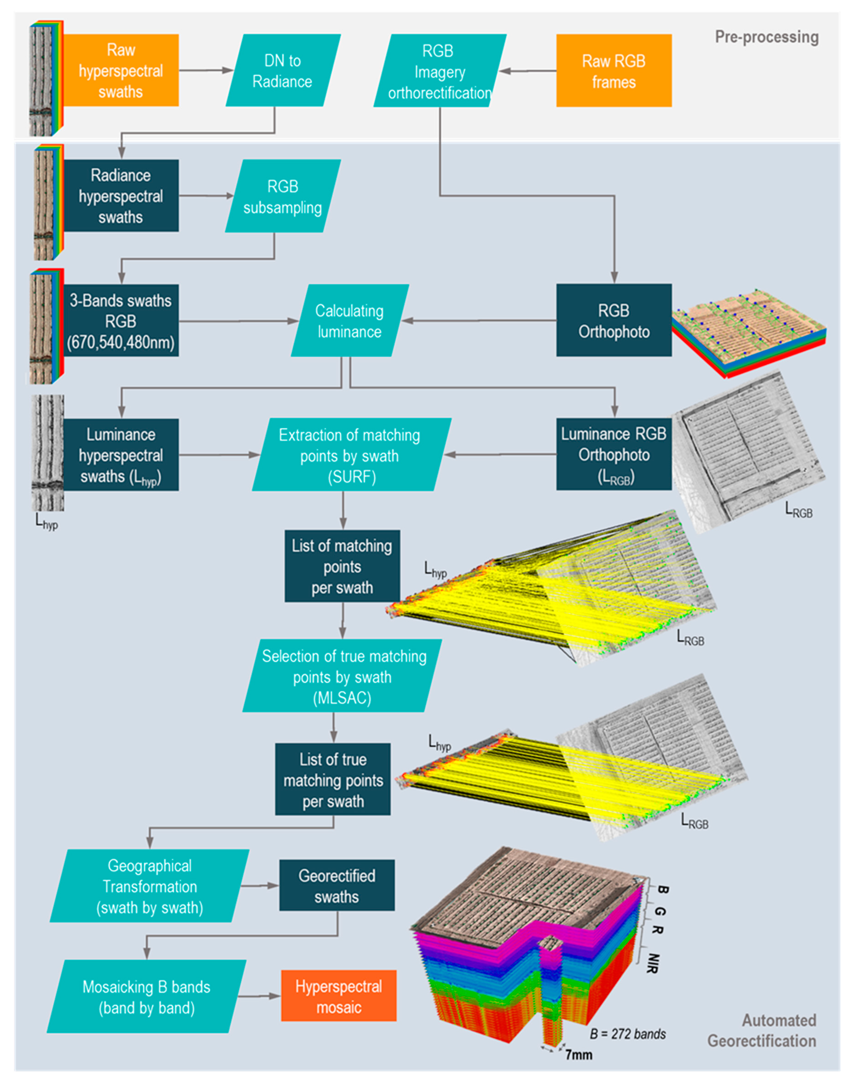
The GNSS receivers fitted on the UAVs record the geographical location of the cameras with decimeter-level accuracy when an image is taken. However, this low geometric accuracy could affect the quality of the imagery and consequently the products derived from them. In order to assure the highest possible geometric accuracy, GCPs were spaced throughout each area of interest, surveying their center coordinates using a Leica Viva GS15 rover [57] and a RTK Leica AS10 GNSS base station [58]. All raw data from the base station and rover were postprocessed using Leica Geo Office package [59]. For the tomatoes field, five checkerboards of dimension 1 m × 1 m were used as GCPs, with four placed in each corner and one in the center of the field. For the date palms, three circular targets of 0.5 m diameter were spaced throughout the area of interest.

3. Methods

Raw remote sensing imagery is comprised of row and column coordinates pairs, i.e., pixels do not have preassociated geographic coordinates. Unprocessed images present geometric and location distortions that must be corrected through a process known as georectification. This process combines two key steps including rectification, whereby pixels are transformed to a common plane that corrects for geometric distortions; and georeferencing, where real-world coordinates are assigned to each pixel of the image. For an accurate georectification, an automated coregistration methodology between preprocessed hyperspectral scans and RGB orthorectified images is proposed herein (Figure 4). Under this approach, the pixel geometry and location in each data-cube is defined by its corresponding pixel in the RGB base image, which has been previously orthorectified using a digital elevation model reconstructed from a Structure from Motion technique (SfM) [60]. The automated georectification workflow was fully coded in Matlab and performed under a parallel computing scheme to speed up data processing. The desktop analysis employed an Intel Xeon E5-2680 v2 processor, 20 cores @2.8 GHz, and 200 GB RAM. The following sections describe the proposed methodological workflow to rectify, georeference, and ultimately to mosaic UAV-based hyperspectral imagery.

3.1. RGB Imagery Orthorectification

The RGB data was processed in Agisoft PhotoScan Professional 1.3 [61] to produce a georeferenced orthomosaic for each experimental campaign. The digital photogrammetric routine implemented in Photoscan [62] includes several stages [63] based on SfM and computer vision algorithms. First, the frame camera positions measured by the GNSS/IMU sensors onboard the M100 aircraft and the set of matching points generated between overlapping images were used in a bundle adjustment to perform the imagery alignment. The default number of key and tie points, 40,000 and 4,000 pairs, respectively, were used to retrieve an initial cloud of matches. Then, the external and internal orientations of the frame camera were estimated. Based on the camera positions and a minimum of three GCPs manually identified, a dense cloud of georeferenced 3D points was generated and interpolated over the area to produce a digital elevation model (DEM) and an RGB orthomosaic. Ultra-high accuracy and moderate depth filtering options were set to discriminate most of the outlier points and retrieve the dense cloud. Because the GSD reached by the orthomosaics was smaller than the hyperspectral imagery GSD (Table 1), the orthomosaics were resampled to the hyperspectral pixel size by applying a bilinear interpolation, where the output pixel value is estimated by averaging the four surrounding pixels.

3.2. Raw Hyperspectral Data Preprocessing

Nonsystematic distortions are common in airborne sensing. For instance, turbulence and eddy-induced effects during the flight can cause scale and location errors, since the sensor direction and height above ground level varies while scanning. Initial preprocessing of the raw hyperspectral swaths was performed to correct for such distortions by using a parametric model developed by Headwall [40]. Under this approach, the difference (θ) between the effective view angle vector (V) and the theoretic view angle vector (Vt) is calculated by modeling the three-dimensional movements of the aircraft, i.e., roll (ω), pitch (φ), and yaw (κ), which are recorded by the onboard IMU (see Figure 5). This formulation considers adjustment features such as GPS coordinates, timestamps, IMU offsets, the field of view (FOV), lens parameters, and sensor orientation, to reconstruct the scanning geometry line by line and to compose each individual swath. However, this reconstruction approach is limited by the GPS/IMU accuracy leading to geometric errors in the preprocessed scans [28], hence requiring additional processing.

3.3. Luminance Retrieval

Grayscale images are preferred over colored ones in order to simplify the image processing complexity, by transforming an RGB color image into a single channel image. Moreover, grayscale images contain the brightness, contrast, edges, shapes, contours, textures, perspective, and shadows of the original RGB data, easing the matching process between two scenes. From the variety of grayscale approaches, luminance images are considered as the best option to identify potential matching points in scenes composed of homogenous textures [64]. In this study, the RGB mosaic was converted to a grayscale luminance image (Lrgb) by eliminating the saturation and hue information, while retaining the original luminance, using the formulation defined in the international standard National Television System Committee (NTSC) [65] (1). Contrast enhancement of the luminance image was then performed using a histogram equalization process.
L   =   0.299 R   +   0.587 G   +   0.114 B   ,
A luminance image was also retrieved via an RGB composite from each preprocessed hyperspectral swath (Lhyp) by extracting the central wavelength red, green, and blue bands (670 nm, 540 nm, and 480 nm).

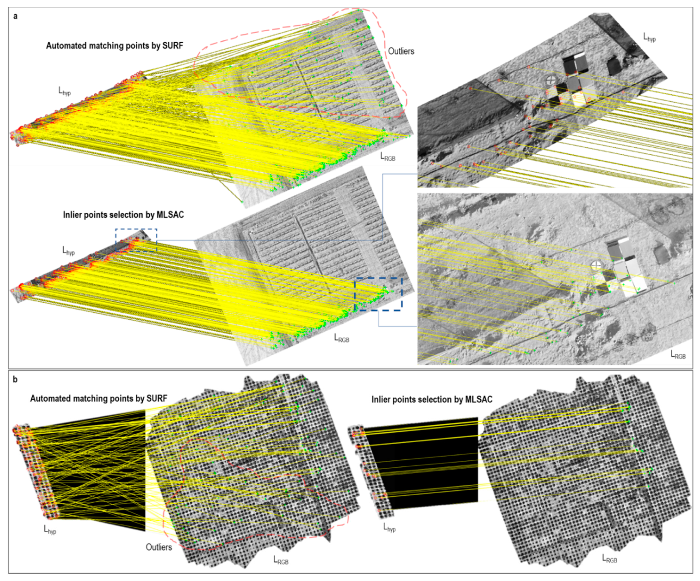
3.4. Extraction of Matching Points by SURF

An implementation of the Speed Up Robust Features (SURF) [48] computer vision technique was used to align the Lhyp based on corresponding points from the Lrgb. SURF is implemented since it is widely used as a scale-invariant feature detector method that is able to retrieve both matching points position and their correspondent descriptors. SURF performs the matching points (or features detection) by following three main stages: (i) extraction, (ii) description, and (iii) matching. Edges, corners, blobs, ridges, or any other specific pattern is considered as a feature, with the only condition to be unique, easily tracked, and comparable. First, the locations of key points that are likely to be found in both images are extracted by convolving two-dimensional box Gaussian smoothing filters, vertically and horizontally, with the integral images of Lhyp and Lrgb, which are an averaged version of the luminance L commonly used to speed up the convolution calculation. Thus, feature orientations are defined by the vector sum of vertical and horizontal responses for the neighborhood around each point. This process is done in parallel for different scales by using filters with different sizes, increasing the chances to detect both smaller and larger sized features, and identifying in this way, scale and rotation invariant key points such as corners, blobs, and T-junctions. The results of these convolutions are integrated into a Hessian matrix per each point. Then, a new neighborhood window is oriented along the dominant direction of each point, and by dividing each window into 4 × 4 sub-regions, horizontal (Σdx) and vertical (Σdy) Haar wavelet responses are again taken to form a vector descriptor V (2), which describes the luminance (L) distribution and polarity (Σ|dx|, Σ|dy|) of the surrounding pixels. Finally, the sign (-, +) of the Hessian matrix trace is used to classify bright features on dark backgrounds and dark features on a bright background. Only features from both images, Lrgb and Lhyp, with identical sign are compared, and the Euclidian distance between their descriptor vectors is calculated to select the set of matching points.
V   =   ( Σ dx ,   Σ dy ,   Σ | dx | ,   Σ | dy | )   ,

3.5. Selection of True Matching Points by MLSAC

The set of paired points obtained by SURF can contain both true and false feature matches, affecting the accuracy of the fitted geographical transformation. To address this, a parameter estimation approach is required, that adjusts the best transformation model from outlier-corrupted data. Here, we use the Maximum Likelihood Sample Consensus (MLSAC) [49] algorithm, which is an adaptation of the widely applied Random Sample Consensus (RANSAC) technique. RANSAC [66] is a hypothesis-verify iterative method used in coregistration applications to estimate model (projective, affine, etc.) parameters that best fit the set of paired points (true and false) retrieved by a feature detector (SIFT, SURF, etc.). It proceeds by repeatedly generating and testing solutions estimated from a minimal random set of matches gathered from the total paired points. The best solution relies on the highest number of true matches (inliers), with an error below a user-defined threshold. In contrast, MLSAC adopts the same iterative strategy to generate solutions from random samples of matches, but chooses the solution that minimizes the error, rather than just looking for the maximum number of inliers. The following three points motivate that use of MLSAC herein:
  • MLSAC improves upon RANSAC by assuming the distance between paired points follows a Gaussian distribution, with a zero-mean error and a uniform standard deviation.
  • A maximum likelihood cost function is evaluated in terms of finding the solution that minimizes the error.
  • Since the optimal solution does not rely on a defined number of inliers, MLSAC is well suited to estimating complex geometric transformations that exist between images captured under different viewing geometries, where just a few true matches could be retrieved.
MLSAC workflow consists of five general stages. First, a randomly sampled set of matching points is considered to fit an initial transformation model, using the remaining points for testing. Then, each individual matching pair is evaluated by using the fitted model to estimate the distance error in pixels between the point in Lrgb and the projection of the corresponding point from Lhyp. The algorithm classifies as inliers those points whose distance error is below a threshold of N pixels and counts the total number of inlier candidates. The N limit depends on the aimed positional accuracy of the results, which in this case was set to a maximum of 1.5 pixels. Then, the likelihood of the probability distribution function of the errors is maximized, and the above process is repeated i times (3) to evaluate a statistically significant number of subsamples. These i iterations depend on the randomly sampled subset size (m), the percentage of outliers (w) allowed, and the probability of selecting a good subsample (q). Generally, a probability q = 99% is desired, considering w = 50% as the worst case scenario, and m = 3, or m = 4 when using an affine or projective transformation, respectively. After the loop is finished, the transformation model that maximizes the likelihood of the cost function with a 99% confidence of finding the maximum number of inliers is selected as the best solution.
i =   log ( 1 q ) log ( 1 w m )

3.6. Geographical Transformation and Mosaicking

Affine transformation, a special case of the projective approach, was used to convert the Lhyp units to real-world coordinates, based on the Lrgb mosaic, since it is one of the most flexible transformation methods (4) [67]. This transformation model requires a minimum of three pairs of matching points to translate, scale, shear, and rotate an image while preserving parallelism. Generally, the greater the number of true matching pairs, the higher the accuracy of the model.
[ x y 1 ] =   [ x y 1 ] [ a 1 a 2 t x a 3 a 4 t y 0 0 1 ]
where x and y are the coordinates of the transformed point, x and y are the original coordinates of the point, a 1 , a 2 , a 3 , and a 4 define linear transformations composed by scale, shear, and rotation factors, and t x and t y specify the displacement or translation along the X and Y axis, respectively.
By running the routines previously described, individual geographic transformation solutions per swath were determined and operated band by band. Finally, the hyperspectral mosaic is produced by merging one by one these multiple georectified swaths into a single mosaic per band and stacking together these individual mosaics into a raster data cube, where the output pixel values for the overlapping areas are determined by the value from the last swath added into the mosaic.

3.7. Georectification Assessment

The relative positional accuracy between each georectified hyperspectral dataset and the correspondent RGB mosaic was determined by calculating the root mean square error (RMSE), the mean absolute error (MAE), and the accuracy at the 95% confidence limit. The RMSE (5) is determined by calculating the Euclidean distance between the rectified coordinates in the hyperspectral mosaic and the reference coordinates in the RGB mosaic. The closer the RMSE values are to zero, the more accurate the georectification. In this case, the reference coordinates were prespecified check points from each of the imagery. Check points are identifiable features in both the reference RGB image and the hyperspectral mosaic, whose locations are used to quantitatively assess the positional quality of the georectified data cube. To compute the RMSE, at least 20 well-defined checkpoints are used per mosaic, making sure that 25% are well distributed in each of the four quadrants of the image of interest (for the tomato experiment). A total of 52 (tomato) and 25 (date plantation) checkpoints were randomly spread over each dataset.
R M S E =     1 n i = 1 n ( ( x h y p x r g b ) 2 + ( y h y p   y r g b ) 2 )
The MAE [68] (6) measures the average magnitude of the Euclidean distance in the set of checkpoints, where all individual differences have equal weight.
M A E   =   i = 1 n ( ( x h y p x r g b ) 2 + ( y h y p   y r g b ) 2 ) n ,
According to the National Standard for Spatial Data Accuracy (NSSDA) [69,70], the relative horizontal positional accuracy is reported in meters at the 95% confidence level (9) and is determined in two separate components: x (7) and y (8). The value of 1.22385 in the accuracy expression in (9), is derived from the Chi-square statistical distribution for 2 degrees of freedom and a lower tail area of 0.05. In other words, 95% of the positions in the hyperspectral mosaic will have an error with respect to the RGB mosaic position that is equal to, or smaller than, the reported accuracy value.
R M S E x =     1 n i = 1 n ( x h y p x r g b ) 2   ,
R M S E y =     1 n i = 1 n ( y h y p y r g b ) 2     ,
A c c u r a c y 95 % =   1.22385   ×   ( R M S E x +   R M S E y   )   ,
In addition, the performance of the proposed automated method was evaluated with respect to a semiautomated approach by manually selecting matching points between the hyperspectral swaths and the RGB image. The number of good matches (or inliers) retrieved by the automated workflow was used as a reference to set the number of point pairs to be identified by hand and to fit an affine transformation per swath. The aligned strips were mosaicked together, and the above-mentioned positional accuracy metrics were estimated to compare the performance of both methods.

4. Experimental Results and Analysis

The UAV-based hyperspectral imagery for both field experiments was georectified and mosaicked using the methodology described above. In this section, the efficiency of the automated coregistration routine between hyperspectral data and RGB frame-based imagery is evaluated, together with a qualitative and quantitative assessment of the accuracy reached for the georectified high spatial and spectral resolution mosaics. An analysis of the computational cost of the automated process is also undertaken.

4.1. RGB Frame-Based Orthomosaic

As described in the previous section, the RGB orthomosaics derived from the collected frame images were processed using a SfM package and GCPs. All the mosaics over the tomatoes field (Figure 6a) were resampled from 0.005 to 0.007 m, with a rectification error of 0.002 m. Similarly, the native resolution of the date palms mosaic (Figure 6b) was resized from 0.034 to 0.060 m, with an RMSE error of 0.043 m. From visual inspection of these images, in general a good alignment was reached by the RGB mosaics, well preserving sizes and shapes. Figure 6a shows how some linear features are continuous, such as irrigation pipes, defined objects like individual plants are free of gaps or blur effects, and contrasting tones and textures are visible in the bare soil areas. From Figure 6b, road edges are continuous and well defined, date palms keep their characteristic shapes, and soil areas preserve smooth textures and contrasting tones.

4.2. Efficiency of the Automated Coregistration Routine

The most important steps in the coregistration processing are the extraction and selection of common features between the RGB reference image and each preprocessed hyperspectral swath. Under the proposed methodology, SURF was used to extract a set of matching points, which were purged of false positives or outlier pairs by using the MLSAC model. The efficiency of these combined routines relies on the number of inliers retrieved to fit the best affine transformation function, to align each swath to the RGB mosaic. The higher the number of inliers, the better the fitting of the transformation model. Table 2 presents the number of features detected in the RGB mosaics and the average detected per swath, together with the matches identified by SURF, and the total inliers selected by MLSAC. It is evident how the features retrieval varies from one flight to another, since this process is performed by using luminance images, which in turn vary with the illumination and surface conditions. Although a large number of features were extracted, from 10K in the hyperspectral data to 300K in the RGB approximately, only few matches were retrieved, between 505 and 951 pairs in the case of the tomato crop, and 103 pairs in the date palms dataset. This performance is explained not only by different illumination conditions but also when coregistering data from different sensors [71]. In the case of the tomato field experiments, the percentage of points pairs detected as inliers from the total of matches varies between 65% and 80%. An average of 26% of matches was selected as inliers for the date palms swaths. In both cases, the number of inliers was sufficient to fit the transformation models by swath and to ultimately stitch the hyperspectral mosaics.
Both the number of inliers and the distribution of the points along the swaths are determinant by the georectification quality. Inliers should be fairly uniform and located across the strips in order to avoid local distortions after performing the geometric transformation. Figure 7 shows some examples of the distribution and location of the matching points extracted by SURF, from which MLSAC selected the set of inliers. In the case of the tomato crop (Figure 7a), a dense cloud of matches was retrieved, including some outliers that are generated when the texture, color, or intensity of the surface are homogeneous, thus identifying similar patches between the hyperspectral strip and the RGB reference. After MLSAC prunes the false matches (or outliers), a good distribution of inliers is achieved. Figure 7a shows a close-up of an area where some calibration panels and GCPs were placed and where a good number of inliers were selected. However, the number of matches can decrease when repetitive forms are present within the images, i.e., the neighborhood around the features does not vary enough to allow for reliable comparison between both scenes. An example of this effect is shown in Figure 7b, where the crown of the palms represents a very homogeneous pattern. In this case, the density of matches is reduced, but the extracted inliers are still well distributed across the swath.

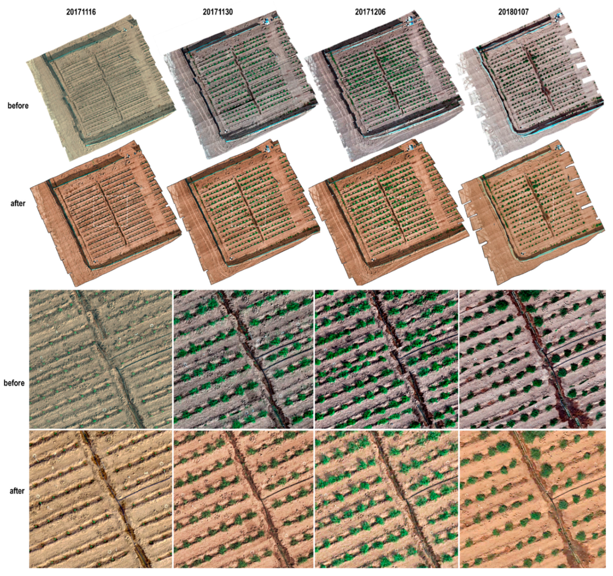
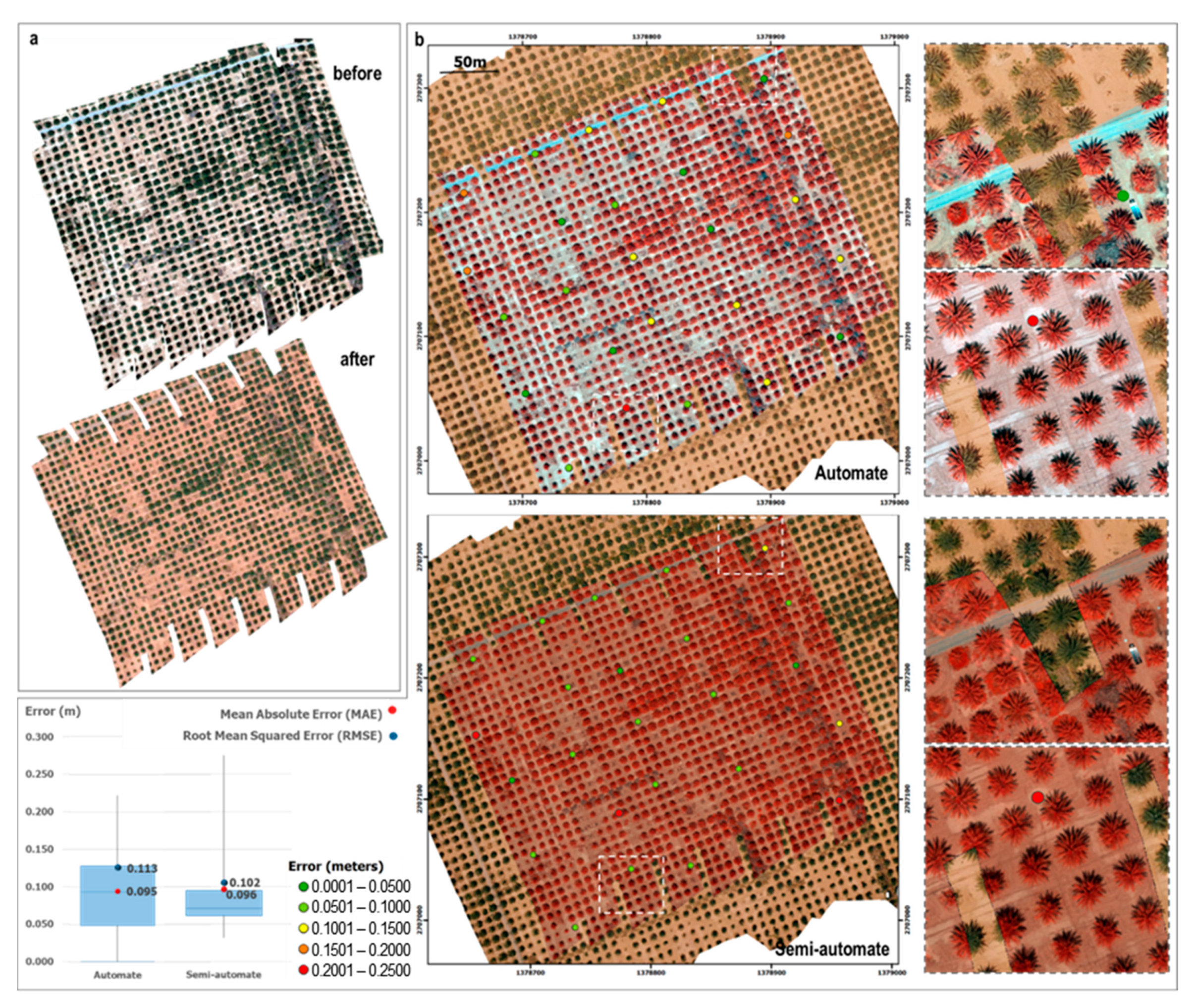
4.3. Qualitative Accuracy Assessment

As part of the accuracy assessment of the results, an evaluation of visual factors such as gaps, matches across boundaries, deformations, and patches was performed. Figure 8 shows a comparison between the preprocessed and the georectified multitemporal hyperspectral mosaics for the tomato experiment. As can be seen, the full dataset is free of gaps and patches, and the hyperspectral swath borders are dissembled. In the zoomed areas, the impact of the automated alignment can be seen on some linear features, such as irrigation pipelines, furrows, and fences, which are straight, parallel, or continuous across the stitched swaths. Likewise, the shapes and sizes of individual plants are well maintained. The high degree of visual consistency achieved indicates that the estimated affine transformations were well fitted with sufficient and well-distributed corresponding points.
For the case of the date palms experiment, the misalignment between preprocessed passes can clearly be seen in Figure 9, with overlapping distortions of individual palms. After processing, a good fit between the RGB reference and the hyperspectral georectified mosaic was reached. The matching quality of linear geometries, such as the border of the roadway (Figure 9b), or the continuity of leaflets in the crown of the palms can be observed throughout the mosaic. As with the tomato experiment, the collinearity and equidistance between individual palms were recovered by the georectification process. Particularly noticeable is the good performance of the affine transformations at the extreme borders of the swaths, which are usually susceptible to deformation when insufficient or poorly-distributed stitching points are retrieved. While the automated routine produced a lower number of matches in this case than for the tomatoes experiment, the set of inliers was sufficient to fit a highly accurate transformation model.

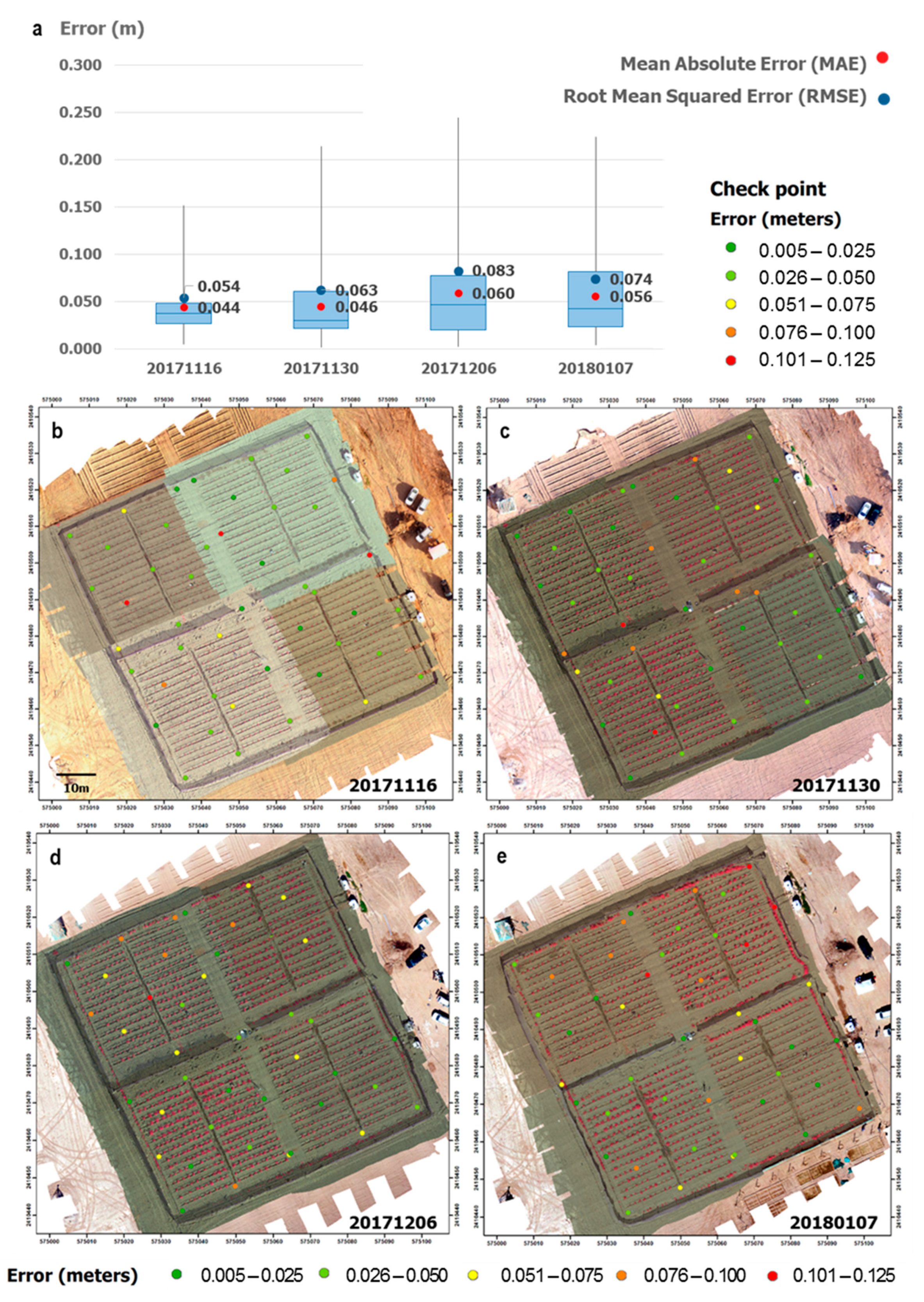
4.4. Spatial Accuracy

Although the visual inspection of the hyperspectral mosaics provides an important qualitative indication of the spatial accuracy, quantifying statistical metrics such as the mean absolute error (MAE), root square mean error (RMSE), and relative positional accuracy (Table 3) is necessary to develop confidence in the approach.
Figure 10 illustrates the checkpoints evaluation for the hyperspectral data series in the tomato experiment. The error is randomly distributed over the mosaics, reaching an overall MAE between 6 and 8 times the ground sampling distance (which represents around 5 cm) and an RMSE at the level of 7 to 11 times GSD (corresponding to approximately 6 cm). Figure 9 shows how the error is distributed throughout the checkpoints over the date palms crop. In this case, the MAE and RMSE were at the level of 1 and 1.5 times GSD, which equates to 6 and 9 cm, respectively. However, errors for some of the mosaics are more variable than others, which is the case for the last two datasets in the tomato experiment and single capture for the date palm experiment, showing a direct correlation between the achieved error and the percentage of inliers selected from the total matching points, i.e., the more inliers that are detected (Table 2), the lower the RMSE.
The relative accuracy was tested by comparing the X (east) and Y (north) coordinates of the checkpoints with their correspondent coordinates from the RGB mosaic, which is considered an independent source of higher accuracy. This metric is reported in ground distances to directly compare the results, considering their different spatial resolutions. The accuracy achieved in the tomato experiments throughout the 52 checkpoints and at a 95% confidence level, varies between 9 and 13 cm (Table 3). According to the NSSDA standard, when 50 points are tested, the percentage confidence level allows a maximum of three checkpoints to be above the MAE. This criterion is met for all of the mosaics in the tomato experiments, as shown in Table 3 (last column) and Figure 10 (red points). In the case of the date palm experiment, the accuracy reached throughout the 25 checkpoints at a 95% confidence level, was 18 cm. Following the NSSDA standard for >20 tested points, only one is allowed to be above the MAE, which is a condition achieved by the resulting mosaic (see Figure 9, red points).
An additional spatial quality assessment for the date experiment was performed by comparing a semiautomated georectification with the automated method proposed herein. To do this, matching points between each scanned swath and the RGB-frame reference were manually identified, with a total of 27 stitching points per swath selected (as this number corresponds with the average of inliers retrieved per swath by the automated method; see Table 2). A polynomial affine transformation was performed using these points, achieving an RMSE of 0.102 m, an MAE of 0.096 m, and an accuracy of 0.167 m at a 95% confidence level. Figure 9d,e show the error distribution of the checkpoints achieved for both methods. As anticipated, the error is smaller and more homogenous across the manually-rectified mosaic compared to the automated effort, although the difference in spatial accuracy achieved is around 1 cm.

4.5. Processing Efficiency

Given that the proposed approach can achieve spatial accuracies comparable with those obtained by manually identifying the matching points, one of the key reasons for choosing an automated method will be based on the processing time (i.e., it should be faster and as reliable when compared with manual approaches). The efficiency of an algorithm is usually expressed in terms of its processing time. As such, the computational cost of the proposed automated georectification workflow, coded in Matlab, was measured on a per step basis to allow an intercomparison of the approaches. Some factors, such as 200 GB of RAM memory and 20 processor cores, were set as constant to execute the routines. Table 4 compares the timing measurements per dataset for three general stages: (i) extraction and selection of matching points, (ii) geographic transformation, and (iii) mosaicking. The manual coregistration performed for the date palms imagery was also timed, with an average of 3 min required to manually identify each of the 27 pairs of matching points per swath, from a total of 16 flight lines (i.e., 21.6 h in total). It is noticeable that the time required to execute each stage is correlated with the data size. That is, the larger the data set, the longer the processing time. For the automated solution, nearly 10% of the processing time is used to extract and select the matching points, while another 10% is spent by the geographic transformation. The majority of the time, around 80%, is dedicated to stitching the strips and stacking the bands together into a single hyperspectral mosaic. In contrast, when comparing both approaches (the automated with the semiautomated), a difference of 21.3 h was measured, where 85% of the total time was spent by the handmade selection of points.

5. Discussion

A range of semiautomated [18,20,22,26,41] and fully automated frameworks [37,38,72,73,74] have been explored to georectify UAV-based hyperspectral data captured by push-broom cameras. However, challenges related to data collection procedures, quality assessment, and optimization of algorithms require further investigation to expedite data processing and accomplish a standardized positional accuracy of retrieved data. These factors, together with the need for processing large volumes of image time-series, motivated the development of a simplified, expedited, and automated workflow to georectify and mosaic high-spatial-resolution hyperspectral images acquired by UAV-based push-broom spectroradiometers. To address these challenges, an improved coregistration strategy combining SURF feature detector and MLSAC model-fitting algorithm was established to allow robust direct geographic transformation between the hyperspectral scans and an RGB reference orthophoto. An additional novel aspect of the proposed approach is the fact that high positional accuracies can be reached with different percentages of true matches without requiring any additional image treatment and with a limited number of GCPs.
Some considerations relevant to the development and execution of the proposed methodology must be taken into account to assure an effective implementation for multiple applications. For instance, in the data collection stage, it is advised to design a flight plan that allows the simultaneous collection of coincident hyperspectral and RGB frame-based data. Establishing a minimum of requisites, such as atmospheric conditions, side-lap overlaps, flight speed and height, frame rate scanning, and FOV allows the capture of both datasets under similar illumination conditions and to achieve comparable spatial resolutions. However, if different GSD are collected between the RGB reference and the hyperspectral dataset, then the RGB dataset should be resampled to the hyperspectral imagery resolution, to increase the efficiency of the SURF coregistration method. Although SURF is a scale-invariant feature detector, it has been shown elsewhere that the algorithm operates considerably better when comparing similarly scaled images [75]. An alternative to managing the scale difference was proposed by Habib et al. [38], who established a GSD ratio threshold between the spectral scans and the RGB reference to constrain the feature detection in SURF. However, our study demonstrates that resizing the RGB orthomosaic is enough to retrieve hundreds of matches. Another aspect to account for is the flight time, since the coregistration is based on the similarity of the luminance images derived from the hyperspectral swaths and the RGB orthophotos. Both datasets should be consecutively (or simultaneously) collected in order to avoid significant changes in luminance. Theoretically, SURF or any other type of feature detector/descriptor algorithm always retrieves interest points from an image unless it is a constant matrix whose pixel values are all the same [75]. However, the number of features detected can be reduced by the homogeneity of the scene, since the detection is based on local texture analysis. For instance, a poor number of SURF points could be retrieved for an image covering a highly homogeneous and flat desert area. In such a case, the number of true matches between two scenes could be null if these were captured under slightly different illumination conditions, hence requiring ancillary GCPs. Although SURF is also robust under invariant illumination conditions [48], large differences between the images to coregister (e.g., shadows or new elements placed on the ground) can reduce the number of matches and the georectification quality. Considering such factors will not only help to reduce ground-based collection efforts, but it will also make the data more reliable.
Amongst the different approaches used to georectify and mosaic UAV-based hyperspectral data, those using coregistration methods with RGB scenes from frame sensors generally yield better accuracies and products than those based on dense networks of ground control points (GCP) and manual stitching [22,25]. Habib et al. [38] used the same hyperspectral camera and IMU reference employed in this study, with a 17 mm lens and onboard a fixed-wing UAV, to capture 5 cm GSD swaths with 50% side lap over a crop field. Their approach includes a partial rectification of the hyperspectral scans based on a derived DEM from the RGB frame-based dataset and a coregistration strategy based on a modified version of SURF. Their results achieved relative accuracies between 0.5 to 0.9 m RMSE per swath. Considering the comparable date palm study (6 cm GSD) explored here, the relative accuracy achieved for our georectified mosaic (0.1 m RMSE) improved these results by between 67% and 88%. This improvement relies on the use of luminance images and the integration of SURF and MLSAC. In previous approaches [23,38,39], most establish a comparison between the hyperspectral and the RGB data using a single band (often the red band), thereby omitting radiometric differences of both sensors. In contrast, luminance images are based on a model of a weighted combination of RGB wavelengths that equalizes multiple data sources under a standard metric. By comparing the luminance images derived from the high spectral and the RGB datasets, SURF is able to retrieve thousands of features and hundreds of matching points, as shown in the presented study cases. Furthermore, the strategy of selecting true matches (or inliers) is essential to fit an affine model, especially when the study site has a homogeneous land cover. The alternative proposed by Habib et al. [38] to reduce the number of false matches, was by constraining SURF with some ratios and ranges in the spatial location, scale, and main orientation, achieving a maximum of 350 true matching pairs between consecutive swaths, and fitting an affine model base on them. In contrast, our study implements the MLSAC routine as a strategy to do both, selecting the best matching points or inliers, and fitting the transformation model per swath through a maximum likelihood of the error, where the distance error parameter can be set to be as restrictive as required. In the case of the date palms, only an average of 27 inliers per swath are retrieved, and these are the best points that assure an affine model with an error ≤0.09 m per swath.
One of the aims of automated approaches based purely on computer vision and coregistration algorithms is to reduce field and manual work. Ramirez-Paredes et al. found that navigation and positional data are not required to achieve an alignment line-to-line between the RGB reference and the hyperspectral strips, demonstrating this by combining a light payload sensing system with machine vision algorithms. However, spatial accuracy is the most important factor to evaluate in the georectification and mosaicking process. In order to quantify and minimize the absolute error, GCPs, check points, and onboard navigation sensors are always required. Here, it is demonstrated that an automated method that relies on the RGB reference accuracy, requires just a few well-distributed GCPs (minimum five), high-precision GNSS base stations, and GNSS/IMU sensors integrated with the cameras, to produce high-quality results. Moreover, recent studies [76] have found that a minimum of three GCP/ha are sufficient to assure sub centimeter-level horizontal accuracies when operating similar UAV-based RGB systems at 30 m above the ground approximately. One of our study cases reached absolute accuracies of ~1.5 pixels for RGB orthophotos with 5 mm GSD, and relative accuracies between two and seven pixels for hyperspectral images with millimetric resolution (7 mm). Turner et al. [23] conducted a comparative experiment by using the Headwall Micro-Hyperspec onboard a small multi-rotor UAV, integrated with a dual frequency GNSS antenna, an IMU, and a machine vision camera. Their georectified hyperspectral imagery achieves 2 cm GSD with an absolute accuracy of ~2.5 pixels, by sampling 46 GCPs. Although having a significant level of difference in accuracy, these results support the viability of using an ancillary frame camera and automated coregistration methods in combination with a sufficient quantity of GCPs. Ultimately, the number of required GCPs will depend on the area, the desired accuracy level, the terrain conditions, and the available resources (i.e., equipment, time, people).
In terms of computational efficiency, the robustness of the presented workflow is demonstrated (Table 4) by the parallel implementation of optimized algorithms, following the suggestion of Ramirez-Paredes et al. Although it is not possible to establish a comparison between the automated methods in the literature (since these do not report the process timing and barely describe the computational resources and data size), some aspects can be highlighted regarding the efficiency of some of the adopted algorithms. In comparison with the Habib et al. [38] approach, our method performs the feature detection routine SURF only once, whereas their workflow executes it several times, since there is a feature detection between consecutive swaths, and between the swaths and the RGB orthomosaic. Consequently, under that approach, the computational effort in the extraction and selection of matching points stage could increase considerably as the number of flight lines increases. Another comparison can be established with the geocoding package PARGE [39,77], whose ortho-rectification strategy relies on using navigation data (GNSS/IMU), ancillary sensor information (FOV, scanning frequency), high-resolution digital surface models (DSM), and tens of GCPs, in order to fully reconstruct the geometry of the scanning process. According to Schläepfer et al. [77] the whole processing time that PARGE can take to georectify a typical airborne-based scan of 512 × 2000 pixels at 200 spectral channels, is within about 4 h, achieving submetric accuracies. Based on this performance, it is expected that this approach would require a higher computational and manual effort than the approach proposed herein. Likewise, the SpectralView [40] application provides a quick geometry correction approximation, requiring only a coarse resolution DTM and navigation data to produce georeferenced scans. Based on the preprocessing stage of our study data, one hyperspectral scan of 640 × 2000 pixels with 270 bands can be georeferenced through SpectralView within about 1 h, reaching only a submetric level of accuracy and requiring additional processing (like that proposed herein), in order to obtain consistently high positional accuracies.
Although the presented case studies show this automated approach is a valid, computationally efficient, and accurate alternative to the current variety of georectification methods, some improvements would further strengthen the performance of the methodology. In terms of the extraction and selection of matching points, a further comparative study could explore different possible integrations of new image feature detector methods [75] (like SURF) with model fitting routines [78] (like MLSAC), aiming to strengthen the proposed coregistration strategy. With respect to the spatial accuracy assessment of automated georectification methods, as a best practice, it is suggested to use international spatial quality control tests [69,79] that guide how to decide when the accuracy of the results is sufficient or not, for a specific study purpose. Further work could also involve laying out a dense GCP network over a study site to assess the absolute accuracy of the hyperspectral mosaics, especially for mountainous terrains or nonflat fields. In addition, regarding the computational efficiency of the mosaicking stage, it is advised that efficient stitching and band-stacking strategies that can speed up the creation of the hyperspectral mosaic data cube be explored.

6. Conclusions

In order to address the postprocessing georectification challenges in a timely and computationally efficient manner, a batch processing workflow was presented to produce georectified UAV hyperspectral mosaics captured with push-broom sensors. The approach uses as a reference an auxiliary orthophoto collected with a frame-based camera, which is used to individually coregister each spectral scan. SURF and MLSAC computer vision stitching algorithms were implemented to produce thousands of matching points between the intensity images of the RGB reference and each hyperspectral swath. Affine transformations were estimated to obtain free-distortions scanlines, and to stitch them together as mosaic data cubes. The number of inliers extracted from the matching points is correlated with the accuracy of the results, which demonstrates the importance of the SURF coregistration approach to produce high-quality matches, and the consensus algorithm MLSAC to select the inlier pairs. The methodology was tested with different temporal and high-spatial-resolution scenes collected over two varying landscapes. The hyperspectral mosaics with millimeter spatial resolution (7 mm), achieved centimeter level residual errors, with an RMSE of ~7 cm, MAE of ~ 5 cm, and accuracy of ~9 cm at a 95% confidence level. The hyperspectral dataset with centimetric spatial resolution (6 cm) achieved decimeter level residual errors, with an RMSE of ~11 cm, MAE of ~9 cm, and accuracy of ~18 cm at a 95% confidence level. In terms of the computational complexity of the workflow, SURF and MLSAC provide a robust and highly efficient solution to automate the matching points selection process, assuring enough high-quality points to perform an affine geometric transformation. Additional tests are required for implementing approaches that speed up the mosaicking step, since the composition of a mosaic data cube is computationally intensive. Future work should also focus on testing the proposed approach over different terrains and land surface and atmospheric conditions to further improve the framework.

Author Contributions

Experiments were designed by Y.A., D.T., and S.P., in discussion with M.F.M. and A.L. Data processing was undertaken by Y.A. and Y.M. Exploration and analysis were undertaken by Y.A. The manuscript was drafted by Y.A., with input from M.F.M., D.T., Y.M., and A.L. All authors contributed to the final manuscript production. All authors discussed the results and contributed to the final manuscript production. All authors have read and agreed to the published version of the manuscript.

Funding

This research was supported by the King Abdullah University of Science and Technology (KAUST).

Acknowledgments

The authors thank Matteo Ziliani and Bruno Aragon for their assistance in collecting the UAV data and ancillary measurements.

Conflicts of Interest

The authors declare no conflict of interest.

References

  1. Atzberger, C. Advances in Remote Sensing of Agriculture: Context Description, Existing Operational Monitoring Systems and Major Information Needs. Remote Sens. 2013, 5, 949–981. [Google Scholar] [CrossRef] [Green Version]
  2. McCabe, M.F.; Rodell, M.; Alsdorf, D.E.; Miralles, D.G.; Uijlenhoet, R.; Wagner, W.; Lucieer, A.; Houborg, R.; Verhoest, N.E.; Franz, T.E.; et al. The future of Earth observation in hydrology. Hydrol. Earth Syst. Sci. 2017, 21, 3879–3914. [Google Scholar] [CrossRef] [PubMed] [Green Version]
  3. Warner, T.A.; Cracknell, A.P. Unmanned aerial vehicles for environmental applications. Int. J. Remote Sens. 2017, 38, 2029–2036. [Google Scholar]
  4. Manfreda, S.; McCabe, M.F.; Miller, P.E.; Lucas, R.; Pajuelo Madrigal, V.; Mallinis, G.; Ben Dor, E.; Helman, D.; Estes, L.; Ciraolo, G.; et al. On the Use of Unmanned Aerial Systems for Environmental Monitoring. Remote Sens. 2018, 10, 641. [Google Scholar] [CrossRef] [Green Version]
  5. Aasen, H.; Honkavaara, E.; Lucieer, A.; Zarco-Tejada, P.J. Quantitative Remote Sensing at Ultra-High Resolution with UAV Spectroscopy: A Review of Sensor Technology, Measurement Procedures, and Data Correction Workflows. Remote Sens. 2018, 10, 1091. [Google Scholar] [CrossRef] [Green Version]
  6. Zhang, C.; Kovacs, J.M. The Application of Small Unmanned Aerial Systems for Precision Agriculture: A Review. Precis. Agric. 2012, 13, 693–712. [Google Scholar] [CrossRef]
  7. Honkavaara, E.; Saari, H.; Kaivosoja, J.; Pölönen, I.; Hakala, T.; Litkey, P.; Mäkynen, J.; Pesonen, L. Processing and Assessment of Spectrometric, Stereoscopic Imagery Collected using a Lightweight UAV Spectral Camera for Precision Agriculture. Remote Sens. 2013, 5, 5006–5039. [Google Scholar] [CrossRef] [Green Version]
  8. Roosjen, P.P.J.; Suomalainen, J.M.; Bartholomeus, H.M.; Clevers, J.G.P.W. Hyperspectral Reflectance Anisotropy Measurements Using a Push-broom Spectrometer on an Unmanned Aerial Vehicle—Results for Barley, Winter Wheat, and Potato. Remote Sens. 2016, 8, 909. [Google Scholar] [CrossRef] [Green Version]
  9. Pádua, L.; Vanko, J.; Hruška, J.; Adão, T.; Sousa, J.J.; Peres, E.; Morais, R. UAS, sensors, and data processing in agroforestry: A review towards practical applications. Int. J. Remote Sens. 2017, 3, 2349–2391. [Google Scholar] [CrossRef]
  10. Jakob, S.; Zimmermann, R.; Gloaguen, R. The Need for Accurate Geometric and Radiometric Corrections of Drone-Borne Hyperspectral Data for Mineral Exploration: MEPHySTo—A Toolbox for Pre-Processing Drone-Borne Hyperspectral Data. Remote Sens. 2017, 9, 88. [Google Scholar] [CrossRef] [Green Version]
  11. Adão, T.; Hruška, J.; Pádua, L.; Bessa, J.; Peres, E.; Morais, R.; Sousa, J. Hyperspectral Imaging: A Review on UAV-Based Sensors, Data Processing and Applications for Agriculture and Forestry. Remote Sens. 2017, 9, 1110. [Google Scholar] [CrossRef] [Green Version]
  12. Burkart, A.; Cogliati, S.; Schickling, A.; Rascher, U. A Novel UAV-Based Ultra-Light Weight Spectrometer for Field Spectroscopy. IEEE Sens. J. 2014, 14, 62–67. [Google Scholar] [CrossRef]
  13. Turner, D.; Lucieer, A.; Wallace, L. Direct Georeferencing of Ultrahigh-Resolution UAV Imagery. IEEE Trans. Geosci. Remote Sens. 2014, 52, 2738–2745. [Google Scholar] [CrossRef]
  14. Schickling, A.; Matveeva, M.; Damm, A.; Schween, J.; Wahner, A.; Graf, A.; Crewell, S.; Rascher, U. Combining Sun-Induced Chlorophyll Fluorescence and Photochemical Reflectance Index Improves Diurnal Modeling of Gross Primary Productivity. Remote Sens. 2016, 8, 574. [Google Scholar] [CrossRef] [Green Version]
  15. Garzonio, R.; Mauro, B.D.; Colombo, R.; Cogliati, S. Surface Reflectance and Sun-Induced Fluorescence Spectroscopy Measurements Using a Small Hyperspectral UAS. Remote Sens. 2017, 9, 472. [Google Scholar] [CrossRef] [Green Version]
  16. Zeng, C.; Richardson, M.; King, D.J. The impacts of environmental variables on water reflectance measured using a lightweight unmanned aerial vehicle (UAV)-based spectrometer system. ISPRS J. Photogramm. Remote Sens. 2017, 130, 217–230. [Google Scholar] [CrossRef]
  17. Uto, K.; Seki, H.; Saito, G.; Kosugi, Y.; Komatsu, T. Development of a Low-Cost Hyperspectral Whiskbroom Imager Using an Optical Fiber Bundle, a Swing Mirror, and Compact Spectrometers. IEEE J. Sel. Top. Appl. Earth Obs. Remote Sens. 2016, 9, 3909–3925. [Google Scholar] [CrossRef]
  18. Zarco-Tejada, P.J.; Diaz-Varela, R.; Angileri, V.; Loudjani, P. Tree height quantification using very high resolution imagery acquired from an unmanned aerial vehicle (UAV) and automatic 3D photo-reconstruction methods. Eur. J. Agron. 2014, 55, 89–99. [Google Scholar] [CrossRef]
  19. Calderón, R.; Navas-Cortés, J.A.; Lucena, C.; Zarco-Tejada, P.J. High-resolution airborne hyperspectral and thermal imagery for early detection of Verticillium wilt of olive using fluorescence, temperature and narrow-band spectral indices. Remote Sens. Environ. 2013, 139, 231–245. [Google Scholar] [CrossRef]
  20. Zarco-Tejada, P.J.; Morales, A.; Testi, L.; Villalobos, F.J. Spatio-temporal patterns of chlorophyll fluorescence and physiological and structural indices acquired from hyperspectral imagery as compared with carbon fluxes measured with eddy covariance. Remote Sens. Environ. 2013, 133, 102–115. [Google Scholar] [CrossRef]
  21. Hyperspectral Imaging Sensors. Available online: https://www.headwallphotonics.com/hyperspectral-sensors (accessed on 6 November 2018).
  22. Lucieer, A.; Malenovský, Z.; Veness, T.; Wallace, L. HyperUAS-Imaging Spectroscopy from a Multirotor Unmanned Aircraft System: HyperUAS-Imaging Spectroscopy from a Multirotor Unmanned. J. Field Robot 2014, 31, 571–590. [Google Scholar] [CrossRef] [Green Version]
  23. Turner, D.; Lucieer, A.; McCabe, M.F.; Parkes, S.; Clarke, I. Push-broom hyperspectral imaging from an Unmanned Aircraft System (UAS)-geometric processing workflow and accuracy assessment. ISPRS Int. Arch. Photogramm. Remote Sens. Spat. Inf. Sci. 2017, XLII-2/W6, 379–384. [Google Scholar] [CrossRef] [Green Version]
  24. Malenovský, Z.; Lucieer, A.; King, D.H.; Turnbull, J.D.; Robinson, S.A. Unmanned aircraft system advances health mapping of fragile polar vegetation. Methods Ecol. Evol. 2017, 8, 1842–1857. [Google Scholar] [CrossRef] [Green Version]
  25. Sankey, T.; Donager, J.; McVay, J.; Sankey, J.B. UAV lidar and hyperspectral fusion for forest monitoring in the southwestern USA. Remote Sens. Environ. 2017, 195, 30–43. [Google Scholar] [CrossRef]
  26. Suomalainen, J.; Anders, N.; Iqbal, S.; Roerink, G.; Franke, J.; Wenting, P.; Hünniger, D.; Bartholomeus, H.; Becker, R.; Kooistra, L. A Lightweight Hyperspectral Mapping System and Photogrammetric Processing Chain for Unmanned Aerial Vehicles. Remote Sens. 2014, 6, 11013–11030. [Google Scholar] [CrossRef] [Green Version]
  27. HySpex Mjolnir V-1240. Available online: https://www.hyspex.no/products/mjolnir.php (accessed on 6 November 2018).
  28. Hruska, R.; Mitchell, J.; Anderson, M.; Glenn, N.F. Radiometric and Geometric Analysis of Hyperspectral Imagery Acquired from an Unmanned Aerial Vehicle. Remote Sens. 2012, 4, 2736–2752. [Google Scholar] [CrossRef] [Green Version]
  29. Aasen, H.; Bolten, A. Multi-temporal high-resolution imaging spectroscopy with hyperspectral 2D imagers - From theory to application. Remote Sens. Environ. 2018, 205, 374–389. [Google Scholar] [CrossRef]
  30. Berni, J.A.J.; Zarco-Tejada, P.J.; Sepulcre-Cantó, G.; Fereres, E.; Villalobos, F. Mapping canopy conductance and CWSI in olive orchards using high resolution thermal remote sensing imagery. Remote Sens. Environ. 2009, 113, 2380–2388. [Google Scholar] [CrossRef]
  31. Stagakis, S.; González-Dugo, V.; Cid, P.; Guillén-Climent, M.L.; Zarco-Tejada, P.J. Monitoring water stress and fruit quality in an orange orchard under regulated deficit irrigation using narrow-band structural and physiological remote sensing indices. ISPRS J. Photogramm. Remote Sens. 2012, 71, 47–61. [Google Scholar] [CrossRef] [Green Version]
  32. Torres-Sánchez, J.; López-Granados, F.; Peña, J.M. An automatic object-based method for optimal thresholding in UAV images: Application for vegetation detection in herbaceous crops. Comput. Electron. Agric. 2015, 114, 43–52. [Google Scholar] [CrossRef]
  33. Pérez-Ortiz, M.; Peña, J.M.; Gutiérrez, P.A.; Torres-Sánchez, J.; Hervás-Martínez, C.; López-Granados, F. A semi-supervised system for weed mapping in sunflower crops using unmanned aerial vehicles and a crop row detection method. Appl. Soft Comput. 2015, 37, 533–544. [Google Scholar] [CrossRef]
  34. Hagen, N.; Kester, R.T.; Gao, L.; Tkaczyk, T.S. Snapshot advantage: A review of the light collection improvement for parallel high-dimensional measurement systems. Opt. Eng. 2012, 51, 111702. [Google Scholar] [CrossRef] [PubMed]
  35. Hagen, N.; Kudenov, M.W. Review of snapshot spectral imaging technologies. Opt. Eng. 2013, 52, 090901. [Google Scholar] [CrossRef] [Green Version]
  36. Yuan, H.; Yang, G.; Li, C.; Wang, Y.; Liu, J.; Yu, H.; Feng, H.; Xu, B.; Zhao, X.; Yang, X. Retrieving Soybean Leaf Area Index from Unmanned Aerial Vehicle Hyperspectral Remote Sensing: Analysis of RF, ANN, and SVM Regression Models. Remote Sens. 2017, 9, 309. [Google Scholar] [CrossRef] [Green Version]
  37. Ramirez-Paredes, J.P.; Lary, D.J.; Gans, N.R. Low-altitude Terrestrial Spectroscopy from a Push-broom Sensor. J. Field Robot 2015, 33, 837–852. [Google Scholar] [CrossRef]
  38. Habib, A.; Xiong, W.; He, F.; Yang, H.L.; Crawford, M. Improving Orthorectification of UAV-Based Push-Broom Scanner Imagery Using Derived Orthophotos from Frame Cameras. IEEE J. Sel. Top. Appl. Earth Obs. Remote Sens. 2017, 10, 262–276. [Google Scholar] [CrossRef]
  39. Schläpfer, D.; Schaepman, M.E.; Itten, K.I. PARGE: Parametric geocoding based on GCP-calibrated auxiliary data. Proc. SPIE 3438 Imaging Spectrom. IV. 1998, 3438, 334–344. [Google Scholar]
  40. SpectralView. Available online: http://www.headwallphotonics.com/software (accessed on 5 May 2019).
  41. Habib, A.; Zhou, T.; Masjedi, A.; Zhang, Z.; Evan Flatt, J.; Crawford, M. Boresight Calibration of GNSS/INS-Assisted Push-Broom Hyperspectral Scanners on UAV Platforms. IEEE J. Sel. Top. Appl. Earth Obs. Remote Sens. 2018, 11, 1734–1749. [Google Scholar] [CrossRef]
  42. Chen, Y.H.; Lin, H.Y.S.; Su, C.W. Full-Frame Video Stabilization Via SIFT Feature Matching. In Proceedings of the Tenth International Conference on Intelligent Information Hiding and Multimedia Signal Processing, Kitakyushu, Japan, 27–29 August 2014; pp. 361–364. [Google Scholar]
  43. Shene, T.N.; Sridharan, K.; Sudha, N. Real-Time SURF-Based Video Stabilization System for an FPGA-Driven Mobile Robot. IEEE Trans. Ind. Electron. 2016, 63, 5012–5021. [Google Scholar] [CrossRef]
  44. Jeon, S.; Yoon, I.; Jang, J.; Yang, S.; Kim, J.; Paik, J. Robust Video Stabilization Using Particle Keypoint Update and l1-Optimized Camera Path. Sensors 2017, 17, 337. [Google Scholar] [CrossRef] [Green Version]
  45. Anand, R.; Veni, S.; Aravinth, J. Big Data Challenges in Airborne Hyperspectral Image for Urban Landuse Classification. In Proceedings of the International Conference on Advances in Computing, Communications and Informatics (ICACCI), Udupi, India, 13–16 September 2017; pp. 1808–1814. [Google Scholar]
  46. Shi, Y.; Thomasson, J.A.; Murray, S.C.; Pugh, N.A.; Rooney, W.L.; Shafian, S.; Rajan, N.; Rouze, G.; Morgan, C.L.; Neely, H.L.; et al. Unmanned Aerial Vehicles for High-Throughput Phenotyping and Agronomic Research. PLoS ONE 2016, 11, e0159781. [Google Scholar] [CrossRef] [PubMed] [Green Version]
  47. Hassaballah, M.; Abdelmgeid, A.A.; Alshazly, H.A. Image Features Detection, Description and Matching. In Image Feature Detectors and Descriptors. Studies in Computational Intelligence; Awad, A., Hassaballah, M., Eds.; Springer International Publishing: Warsaw, Poland, 2016; Volume 630, pp. 11–45. [Google Scholar]
  48. Bay, H.; Ess, A.; Tuytelaars, T.; Van Gool, L. Speeded-Up Robust Features (SURF). Comput. Vis. Image Underst. 2008, 110, 346–359. [Google Scholar] [CrossRef]
  49. Torr, P.H.S.; Zisserman, A. MLESAC: A New Robust Estimator with Application to Estimating Image Geometry. Comput. Vis. Image Underst. 2000, 78, 138–156. [Google Scholar] [CrossRef] [Green Version]
  50. Johansen, K.; Morton, M.J.; Malbeteau, Y.M.; Aragon, B.; Al-Mashharawi, S.K.; Ziliani, M.G.; Angel, Y.; Fiene, G.M.; Negrão, S.S.; Mousa, M.A.; et al. Unmanned Aerial Vehicle-based Phenotyping using Morphometric and Spectral Analysis can Quantify Responses of Wild Tomato Plants to Salinity Stress. Front. Plant Sci. 2019, 10, 370. [Google Scholar] [CrossRef] [PubMed]
  51. Aaftab, A.; Burhan, A.; Muhammad, N.; Ihsanullah, D.; Sidra, R. Effectiveness of silicon and irrigation scheduling for mitigating drought stress in sorghum (Sorghum bicolor L.) in arid region of Saudi Arabia. Int. J. Biosci. 2018, 12, 266–278. [Google Scholar]
  52. Aly, A.A.; Al-Omran, A.M.; Sallam, A.S.; Al-Wabel, M.I.; Al-Shayaa, M.S. Vegetation cover change detection and assessment in arid environment using multi-temporal remote sensing images and ecosystem management approach. Solid Earth. 2016, 7, 713–725. [Google Scholar] [CrossRef] [Green Version]
  53. Matrice 600. Available online: https://www.dji.com/matrice600 (accessed on 6 November 2018).
  54. Matrice 100. Available online: https://www.dji.com/matrice100 (accessed on 6 May 2019).
  55. Zenmuse X3. Available online: https://www.dji.com/zenmuse-x3 (accessed on 6 December 2017).
  56. Universal Ground Control Station. Available online: https://www.ugcs.com (accessed on 6 November 2018).
  57. Leica Viva GS15—Smart Antenna. Available online: https://leica-geosystems.com/products/gnss-systems/smart-antennas/leica-viva-gs15 (accessed on 17 May 2019).
  58. Leica AS10 GNSS—Compact Antenna. Available online: https://leica-geosystems.com/products/gnss-reference-networks/antennas/leica-as10 (accessed on 6 November 2018).
  59. Leica Geo Office. Available online: https://leica-geosystems.com/products/total-stations/software/leica-geo-office (accessed on 16 December 2017).
  60. Turner, D.; Lucieer, A.; Watson, C. An Automated Technique for Generating Georectified Mosaics from Ultra-High Resolution Unmanned Aerial Vehicle (UAV) Imagery, Based on Structure from Motion (SfM) Point Clouds. Remote Sens. 2012, 4, 1392–1410. [Google Scholar] [CrossRef] [Green Version]
  61. Agisoft PhotoScan. Available online: https://www.agisoft.com (accessed on 6 November 2018).
  62. Verhoeven, G. Taking computer vision aloft—Archaeological three-dimensional reconstructions from aerial photographs with photoscan. Archaeol. Prospect. 2011, 18, 67–73. [Google Scholar] [CrossRef]
  63. Ziliani, M.G.; Parkes, S.D.; Hoteit, I.; McCabe, M.F. Intra-Season Crop Height Variability at Commercial Farm Scales Using a Fixed-Wing UAV. Remote Sens. 2018, 10, 2007. [Google Scholar] [CrossRef] [Green Version]
  64. Kanan, C.; Cottrell, G.W. Color-to-Grayscale: Does the Method Matter in Image Recognition? PLoS ONE 2012, 7, e29740. [Google Scholar] [CrossRef] [Green Version]
  65. Recommendation ITU-R BT.601-7. Available online: http://www.itu.int/dms_pubrec/itu-r/rec/bt/R-REC-BT.601-7201103-I!!PDF-E.pdf (accessed on 6 November 2018).
  66. Fischler, M.A.; Bolles, R.C. Random sample consensus: A paradigm for model fitting with applications to image analysis and automated cartography. Commun. ACM 1981, 24, 381–395. [Google Scholar] [CrossRef]
  67. Hartley, R.; Zisserman, A. Multiple View Geometry in Computer Vision, 2nd ed.; Cambridge University Press: New York, NY, USA, 2004; pp. 25–64. [Google Scholar]
  68. Sammut, C.; Webb, G.I. Mean Absolute Error. In Encyclopedia of Machine Learning; Springer: Boston, MA, USA, 2011. [Google Scholar]
  69. Geospatial Positioning Accuracy Standards. Part 3: National Standard for Spatial Data Accuracy, FGDC-STD-007.3-1998. Available online: https://www.fgdc.gov/standards/projects/FGDC-standards-projects/accuracy/part3/chapter3 (accessed on 6 November 2018).
  70. ISO 19157:2013 Geographic Information-Data Quality. Available online: https://www.iso.org/standard/32575.html (accessed on 6 November 2018).
  71. Sedaghat, A.; Ebadi, H. Distinctive Order Based Self-Similarity descriptor for multi-sensor remote sensing image matching. ISPRS J. Photogramm. Remote Sens. 2015, 108, 62–71. [Google Scholar] [CrossRef]
  72. Goncalves, H.; Corte-Real, L.; Goncalves, J.A. Automatic Image Registration through Image Segmentation and SIFT. IEEE Trans. Geosci. Remote Sens. 2011, 49, 2589–2600. [Google Scholar] [CrossRef] [Green Version]
  73. Sedaghat, A.; Ebadi, H. Remote Sensing Image Matching Based on Adaptive Binning SIFT Descriptor. IEEE Trans. Geosci. Remote Sens. 2015, 5283–5293. [Google Scholar] [CrossRef]
  74. Liu, J.; Gong, J.; Guo, B.; Zhang, W. A Novel Adjustment Model for Mosaicking Low-Overlap Sweeping Images. IEEE Trans. Geosci. Remote Sens. 2017, 55, 4089–4097. [Google Scholar] [CrossRef]
  75. Tareen, S.A.K.; Saleem, Z. A comparative analysis of SIFT, SURF, KAZE, AKAZE, ORB, and BRISK. In Proceedings of the International Conference on Computing, Mathematics and Engineering Technologies (iCoMET), Sukkur, Pakistan, 3–4 March 2018; pp. 1–10. [Google Scholar]
  76. Oniga, V.-E.; Breaban, A.-I.; Statescu, F. Determining the Optimum Number of Ground Control Points for Obtaining High Precision Results Based on UAS Images. Proceedings 2018, 2, 352. [Google Scholar] [CrossRef] [Green Version]
  77. Schläpfer, D.; Hausold, A.; Richter, R. A Unified Approach to Parametric Geocoding and Atmospheric/Topographic Correction for Wide FOV Airborne Imagery. Part 1: Parametric Ortho-Rectification Process. In Proceedings of the EARSeL Workshop on Imaging Spectroscopy, Enschede, The Netherlands, 11–13 July 2000. [Google Scholar]
  78. Choi, S.; Taemin, K.; Wonpil, Y. Performance Evaluation of RANSAC Family. In Proceedings of the British Machine Vision Conference, Newcastle, UK, 3–6 September 2009; pp. 81.1–81.12. [Google Scholar]
  79. Mesas-Carrascosa, F.J.; Rumbao, I.C.; Berrocal, J.A.B.; Porras, A.G.F. Positional Quality Assessment of Orthophotos Obtained from Sensors Onboard Multi-Rotor UAV Platforms. Sensors 2014, 14, 22394–22407. [Google Scholar] [CrossRef]
Figure 1. Study site locations, including (left) the tomato experiment at the Hada Al-Sham experimental facility (Lat. = 21.797°, Long. = 39.725°), approximately 60 km east of Jeddah, and (right) the commercial date farm near Al Kharj (Lat. = 24.231°, Long. = 47.633°), approximately 200 km southeast of Riyadh.
Remotesensing 12 00034 g001
Figure 2. The DJI Matrice 600 and 100 unmanned aerial vehicle (UAV) systems, sensors, and payload used for data collection over the experimental sites. The Headwall Nano-Hyperspec collects surface radiance in the wavelength range from 400–1000 nm across 270 continuous bands. The Zenmuse X3 camera collects RGB radiance in the visible spectral range across a single 400–700 nm spectral range.
Remotesensing 12 00034 g002
Figure 3. Flight plans and mission areas for (a) the experimental crop of tomatoes, where one flight per quarter of the field was required to cover the total area; and (b) the commercial plantation of date palms, which was covered by a single flight.
Remotesensing 12 00034 g003
Figure 4. The workflow of the proposed methodology is divided into two main stages, preprocessing and automated processing. The preprocessing corresponds to raw data preparation before going through the georectification and mosaicking routine. The automated processing starts with an RGB subsampling from the hyperspectral swaths to calculate the illuminance image, followed by the coregistration strategy phase required to perform the geographical transformation by swath. Then, the set of georectified strips are merged together to retrieve the final hyperspectral mosaic.
Remotesensing 12 00034 g004
Figure 5. Three-dimensional range of motion of the UAV, where ω, φ, κ denote roll, pitch, and yaw angles, respectively. θ represents the difference between the theoretical view angle vector Vt and the effective look angle vector V.
Remotesensing 12 00034 g005
Figure 6. (a) Multitemporal RGB orthomosaics over the tomatoes field and close-ups of one of the quarters of the total area showing the good alignment and high spatial resolution achieved; (b) RGB orthomosaic and close-up over the date palms plantation.
Remotesensing 12 00034 g006
Figure 7. (a) Matches identified by Speeded-Up Robust Features (SURF) and inliers selected by Maximum Likelihood Estimator Sample Consensus (MLSAC) between both the hyperspectral strip (Lhyp) and the RGB reference (LRGB) luminance images in the tomatoes field on 2017/320; (b) matching and inlier points identified between Lhyp and LRGB in the date palms field.
Remotesensing 12 00034 g007
Figure 8. Comparison between preprocessed (before) and rectified multitemporal hyperspectral data (after). Close-ups of a central area show the good alignment achieved by continuous linear features, such as irrigation pipelines and furrows, which were originally shifted before performing the georectification.
Remotesensing 12 00034 g008
Figure 9. (a) Box-plot of the spatial error distribution for the tomatoes case study; (b–e) false infrared composition of the georectified hyperspectral mosaic of the tomato experimental field and positional error for 52 check points.
Remotesensing 12 00034 g009
Figure 10. (a) Comparison of the hyperspectral mosaic before and after the automated georectification; (b) false infrared composition of the georectified hyperspectral mosaic overlapping the RGB base and positional error for 25 checkpoints. Some close-up (right) of two areas show the alignment of a road and the palm crowns.
Remotesensing 12 00034 g010
Table 1. Flights planning and collected data details per campaign.
CropArea (ha)Year/DOYRGB FramesHyperspectral Swaths Per DayHyperspectral Data Size (Gigabytes)Ground Sampling Distance GSD (m)GCPs
Tomato0.642017/32019656232.80.0075
2017/334220.4
2017/340202.2
2018/007274.7
Date Palms8.702018/08718416770.063
Table 2. Features, matches, and inliers detected per flight.
CropYear/DOYRGB FeaturesMetrics Accounting all Swaths per Flight
Hyperspectral FeaturesMatching PointsAverage InliersInliers/Matching
Min.Aver.Max.Min.Aver.Max.(%)
Tomato2017/320309461371353866740199818951108375780
2017/33429301332817351613750563377190859177
2017/34024657529589364874338539350561632765
2018/00730121036145367983745152066781347771
Date Palms2018/0874481568963975010537801031252726
Table 3. Relative positional accuracy assessment of the automated georectification.
CropImage (Year/DOY)Check PointsMin. Error (m)Max. Error (m)MAE (m)RMSE (m)Accuracy 95% (m)# Check Points Whose Error > MAE
Tomato2017/320520.0050.1510.0440.0540.0923
2017/334520.0010.2140.0460.0630.1072
2017/340520.0030.2890.0600.0830.1371
2018/007520.0030.2240.0560.0740.1263
Date PalmsAutomated250.0010.2220.0950.1130.1881
Semi-automated0.0320.2750.0960.1020.1673
Table 4. Georectification processing time by stage.
CropHypers. MosaicMosaic Dimension (Rows × Columns)Mosaic Size (Giga-bytes)Matching Points Extraction and Selection (hours)Geographic Transforma-tion (hours)Mosaicking Time (hours)Net Processing Time (hours)
Toma-toes2017/32016571 × 164292200.60.65.36.5
2017/33416714 × 161431950.50.65.26.3
2017/34016571 × 160001700.40.55.26.1
2018/00716429 × 165712200.60.65.36.5
Date PalmsAutoma-ted8588 × 7758170.30.43.03.7
Semiautomated1721.625

