Article

Potential of Night-Time Lights to Measure Regional Inequality

1
Faculty of Geography, Babeş-Bolyai University, 5-7 Clinicilor street, 400006 Cluj-Napoca, Romania
2
World and Regional Economics Department, University of Miskolc, 3515 Miskolc-Egyetemváros, Hungary
*
Author to whom correspondence should be addressed.
Remote Sens. 2020, 12(1), 33; https://doi.org/10.3390/rs12010033
Submission received: 31 October 2019 / Revised: 10 December 2019 / Accepted: 18 December 2019 / Published: 20 December 2019
(This article belongs to the Special Issue EO Solutions to Support Countries Implementing the SDGs)

Abstract

:
Night-time lights satellite images provide a new opportunity to measure regional inequality in real-time by developing the Night Light Development Index (NLDI). The NLDI was extracted using the Gini coefficient approach based on population and night light spatial distribution in Romania. Night-time light data were calculated using a grid with a 0.15 km2 area, based on Defense Meteorological Satellite Program (DMSP) /Operational Linescan System (OLS satellite imagery for the 1992–2013 period and based on the National Polar-orbiting Partnership–Visible Infrared Imaging Radiometer Suite (NPP-VIIRS) satellite imagery for the 2014–2018 period. Two population density grids were created at the level of equal cells (0.15 km2) using ArcGIS and PostgreSQL software, and census data from 1992 and 2011. Subsequently, based on this data and using the Gini index approach, the Night Light Development Index (NLDI) was calculated within the MATLAB software. The NLDI was obtained for 42 administrative counties (nomenclature of territorial units for statistics level 3 (NUTS-3 units)) for the 1992–2018 period. The statistical relationship between the NLDI and the socio-economic, demographic, and geographic variables highlighted a strong indirect relationship with local tax income and gross domestic product (GDP) per capita. The polynomial model proved to be better in estimating income based on the NLDI and R2 coefficients showed a significant improvement in total variation explained compared to the linear regression model. The NLDI calculated on the basis of night-time lights satellite images proved to be a good proxy for measuring regional inequalities. Therefore, it can play a crucial role in monitoring the progress made in the implementation of Sustainable Development Goal 10 (reduced inequalities).

1. Introduction

At the United Nations (UN) Sustainable Development Summit held in September 2015, the leaders of 193 UN member states expressed their adherence to the 17 Sustainable Development Goals (SDGs) of the 2030 Agenda which, as a global action plan, aims at reducing poverty, fighting inequalities and injustice, and protecting the environment by 2030 [1]. In monitoring progress towards these goals, Earth observation (EO) solutions play an important role in providing information where national data are not available or are costly [2,3,4,5,6,7].
Night-time lights (NTL) satellite images have also been used in a variety of other studies, such as gross domestic product (GDP) estimation [8,9,10,11,12,13], economic decline detection [14,15], ship detection [16], light pollution detection [17,18,19], urban expansion monitoring [20,21,22,23], human well-being measurement [24], built-up area mapping [25,26], modeling of electricity consumption dynamics [27,28,29,30,31], and fire detection [32].
The adoption of the 2030 Agenda with its 17 Sustainable Development Goals (SDGs) created a framework for a radical change in the use of geospatial and EO solutions: 60% of the 169 SDG-related targets and 232 indicators can be directly monitored with EO solutions [4]. SDG 10 aims at reducing inequalities, which include, among other actions, empirical evidence production and monitoring the evolution of inequalities within and among countries. The monitoring of the latter is not difficult for most countries where national accounts and national statistical offices have been established [33]. The difficulties are related to the measurement of sub-national regional inequalities, with two shortcuts: scarce statistical data and a considerable time delay in calculating regional GDPs. Our study links statistical and geospatial frameworks for improved monitoring and reporting on SDG 10. At the same time, to our knowledge, this is the first attempt to introduce EO solutions in measuring SDG 10 at the sub-national level.
We chose Romania as the study area for three reasons: it is one of the most unequal countries of the European Union (EU) [34,35,36,37,38,39,40]; these regional inequalities have been generated in the last 20 years [41,42,43]; and the country has started an economic development process from a low level, making it very suitable for the application of night-time light data from satellite imagery [44]. However, the results are not limited to the area of study, as will be shown in the following parts of the article.
The literature on regional inequalities focused until recently on local tax income from household surveys and GDP per capita from national accounts, as a complex measure of economic development highlighting inter-regional differentials worldwide [34,45,46,47,48,49,50,51,52,53] or applying case studies in a Romanian context [34,35,36,42].
However, the above-mentioned economic indicators used to measure regional inequalities have several limitations, such that GDP is measured directly only at the national level, while at the regional level it is calculated indirectly with a two-year delay compared to the national one [3,54]. Compared to traditional statistical data, night-time lights satellite images have a number of advantages: regional inequality can be calculated locally in real time (instead of waiting two years for the indirect calculations from national accounts); they have higher temporal resolution; and they can be obtained free of charge. Lately, some studies have focused on the use of night-time light data in measuring regional inequalities [54,55,56,57,58,59]. Xu [56] used population density and night-time lights (NTL) satellite images to measure regional inequality of public services at four different scales in China (national, economic regions, provinces, and prefectural cities) and their changes between 2005 and 2010. Zhou [54] analyzed the socio-economic inequality at the subnational level in China, calculating three inequality indices based on the methodology used to calculate the Gini coefficient, the Theil index, and the Lorenz asymmetry coefficient. They found that the Gini and Theil indices at the provincial level were lower than the indices obtained at the county level, and thus obtained a positive statistical correlation between Visible Infrared Imaging Radiometer Suite (VIIRS) night-time radiance and GDP and population.
Although in the last decades a series of studies have dealt with the issue of regional inequalities, there is a large research gap focusing on subnational scales. The purpose of our study is to measure regional inequality in Romania, for the 1992–2018 period, at the county level (NUTS 3 units), using night-time lights (NTL) satellite images, in order to monitor progress in the direction of SDG 10 (reduced inequalities).

2. Study Area and Data

2.1. Study Area

In this study, we analyzed regional inequalities at the county level (NUTS-3) in Romania. Romania is divided into 42 administrative counties (NUTS-3, 41 counties and the Municipality of Bucharest), which are grouped into eight development regions (NUTS-2) used in particular to coordinate regional development projects. The counties are divided into 3181 territorial administrative units (local administrative units (LAU1)): 103 municipalities, 217 cities/towns, and 2861 communes (Figure 1).

2.2. Data Collection

2.2.1. DMSP Night-Time Light Data

The Defense Meteorological Satellite Program (DMSP) satellite images were collected by the National Oceanic and Atmospheric Administration (NOAA). They are available free of charge for the 1992–2013 period and have a spatial resolution of 30 arc s (1 km) (Table 1).
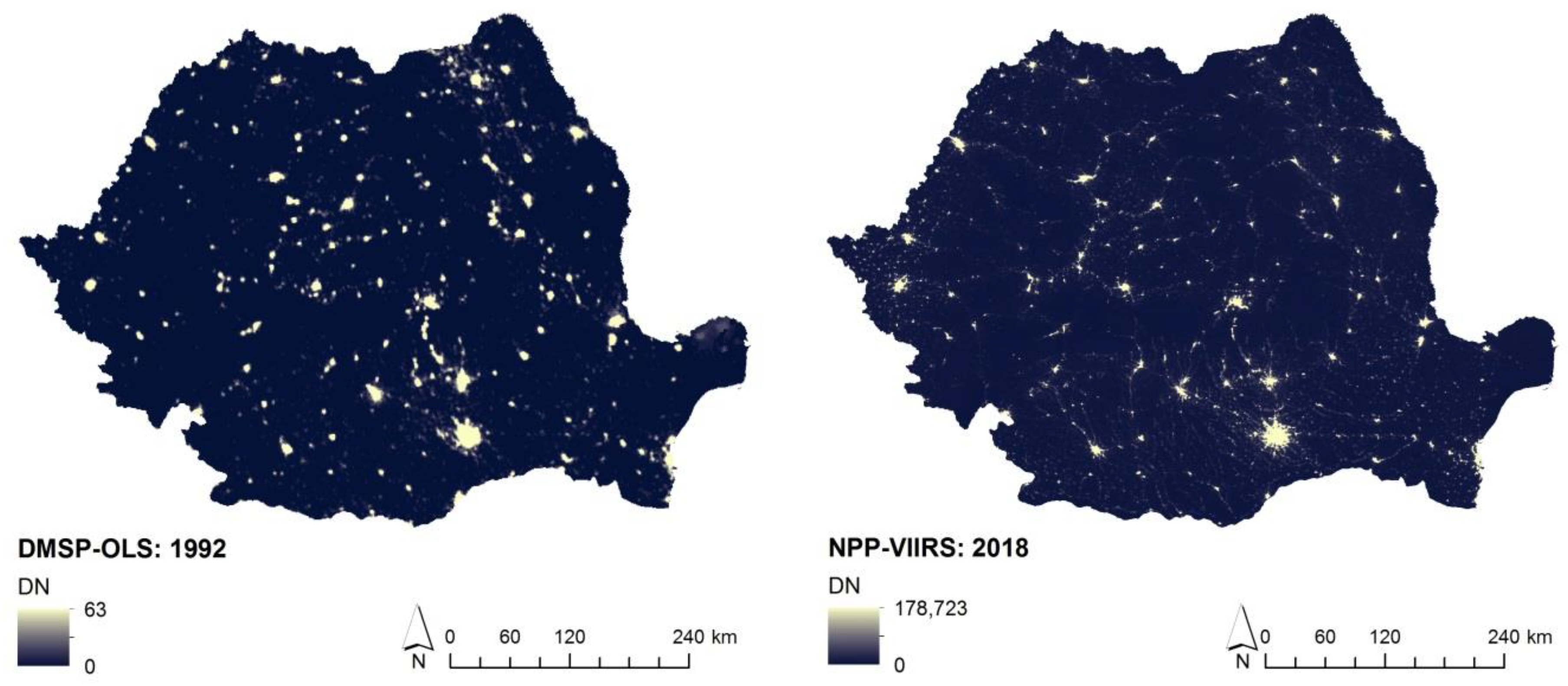
DMSP-OLS satellites orbit the Earth and record the intensity of light using OLS sensors. The light intensity measured by the DMSP-OLS satellites ranges from 0 to 63. Digital number: 0 corresponds to non-illuminated areas, and the 63 values correspond to the strongly illuminated areas (Figure 2). The DMSP images for Romania were extracted from the NOAA/NGDC database Version 4 DMSP-OLS Night-time Lights Time Series [60]. Abbreviations: DMSP, Defense Meteorological Satellite Program; OLS, Operational Linescan System; NTL, night-time lights; NPP, National Polar-orbiting Partnership; VIIRS, Visible Infrared Imaging Radiometer Suite; DNB, day/night band.

2.2.2. NPP-VIIRS Night-Time Light Imagery

The NPP-VIIRS satellite images were collected by the National Oceanic and Atmospheric Administration and National Aeronautics and Space Administration (NASA). The Suomi National Polar-orbiting Partnership (NPP) satellite records light intensity using VIIRS (Visible Infrared Imaging Radiometer Suite) sensors, which collect data in 22 different spectral bands, one of which is the DNB (day/night band). These data are available at an annual scale for 2015 and 2016, and a monthly scale for the 2012–2019 period; their resolution is 15 arc-s (approximately 500 m). In this study, we used Version 1 VIIRS Day/Night Band Night-time Lights suite produced by the Earth Observations Group (EOG) at NOAA/NCEI (National Centers for Environmental Information) [61]. From the annual data we used the "vcm-orm-ntl" layer (VIIRS Cloud Mask–Outlier Removed–Night-time Lights) for 2016, which contains cloud-free average emitted radiance expressed in nW/cm2/sr; these data were subject to an outlier removal process to filter out fires and other ephemeral lights. As regards monthly data, there are two configurations of the NPP-VIIRS composites: “vcmcfg”—data contaminated by stray light are removed, and “vcmslcfg”—data contaminated by stray light are corrected [59]. Thus, for 2014 and 2018, the averaging pixel brightness was calculated based on the monthly data (“vcmslcfg”) corresponding to the summer months (May–September), and two composite VIIRS night-time light images resulted. We used the summer months (May-September) because there were no areas covered in snow in Romania during this period.
The night-time light data were extracted using the ArcGIS 10.1 software, at the level of equal cells of 0.15 m2, based on DMSP/OLS satellite images for 1992–2013 and NPP-VIIRS satellite images for 2014–2018. The DMSP and the NPP-VIIRS data were aggregated on a spatial grid of 0.15 km2 using the Zonal Statistics tool in ArcGIS software. With this tool, a mean statistic was calculated for each grid cell of 0.15 km2 (earlier defined) based on values from NTL data. The NLDI was calculated using the MATLAB software for 41 counties for the 1992–2018 period. The geographical variables (altitude, latitude, and longitude) were deviated from DEM SRTM (Digital Elevation Model - Shuttle Radar Topography Mission) by 90 m.

2.2.3. Demographic and Economic Data

The data on the population of villages, cities/towns, and municipalities (LAU2) were taken from the 1992 and 2011 population census [62]. These data were aggregated on equal grid networks of 0.15 km2; two population density grids were created with the ArcGIS and PostgreSQL software and later used to calculate the NLDI. In the absence of other sources of population data at the local level, the population density grid obtained for 1992 was used to calculate the NLDI for 1992, and the population density grid resulted for 2011 was used to calculate the NLDI for 2008, 2012, 2013, 2014, 2016, and 2018. The population and migration data at the county level for each year were obtained from the National Institute of Statistics [63].
The data on GDP per capita at the county level were extracted from the Eurostat database [64] for the 2008–2016 period, and from the National Institute of Statistics [63] for 1995 (since it was the closest year to 1992 available). The local tax income data at the county level were obtained from the Ministry of Regional Development and Public Administration (MRDPA) [65,66] (Table 2).

3. Methodology

Earth observation allowed us to calculate the Night Light Development Index (NLDI) which we used to measure regional inequality. This index is calculated based on the methodology for the calculation of the Gini coefficient, commonly used to measure regional inequality [43,48,53,67].
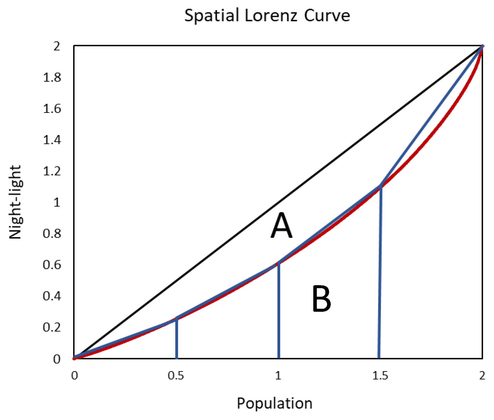
In this study, we intended to measure regional inequalities in Romania using the Night Light Development Index (NLDI), which can be regarded as a proxy variable in highlighting inter-regional differentials [54]. The Gini coefficient is one of the most commonly used indices worldwide for measuring income inequalities among individuals or households in a country. It ranges from 0 to 10, 0 representing perfect equality and 10 perfect inequality. Using the Gini coefficient approach, first we calculated the Night Light Development Index (NLDI) at county level based on data on the spatial distribution of the population and the aggregate night-time light, both at the grid level. Next, we determined the Night Light Inequality Index (NLII) at the national level, based on the Night Light Development Index (NLDI) values at the county level, using the Gini coefficient methodology. The values of the NLII range from 0 to 10, where 0 indicates perfect equality and 10 perfect inequality. The large volume of data required the automation of the NLDI calculation; to this end, a script was developed in MATLAB, and later we integrated therein the gini.m script created by Lengwiler [68]. Gini.m calculates the Gini coefficient (NLDI in our case) and the Lorenz curve using vectors of equal length and values greater than or equal to 0. NLDI values range from 0 to 1, the highly developed counties have low NLDI values and the least developed counties have high NLDI values [55]. The Lorenz curve is the graphical representation of the distribution and it is a straight line in the case of perfect equality (Figure 3).
NLDI = A/(A + B)
because A + B = 0.5 (since the axes scale from 0 to 1).
NLDI = 1 − 2B
where NLDI is the Night Light Development Index; A is the area between the perfect equality line and the Lorenz curve; B is the area under the Lorenz curve.
The NLDI is determined using the calculated area between the Lorenz curve and the axes (B). This area is calculated by computing the average of the left and right Riemann-like sums (rrapezoidal rule). These are called Riemann-like sums because they are calculated in points given by population values and not on a uniform grid (Figure 3).
This area calculation method is commonly used in mathematical analysis to approximate a definite integral. The values of the f function over an interval are approximated by the average of the values at the left and right extremities. A simple calculation involves using the trapezoidal area formula:
A = ½ * h (b1 + b2)
where h is the height of the trapeze; b1 and b2 are parallel sides.
1 2 Δ x [ f ( a ) + 2 f ( a + Δ x ) + 2 f ( a + 2 Δ x ) + 2 f ( a + 3 Δ x ) + + f ( b ) ]
where the interval [a, b] is divided into n subintervals, each of length: Δx = (b − a)/n. The points in the partition will then be: a, a + Δx, a + 2 Δx, ….a + (n − 1) Δx, b.
Using the Gini coefficient approach, the Night Light Inequality Index (NLII) was determined at the county level based on the Night Light Development Index (NLDI) values. In addition, we compared the evolution of the NLII for 1992–2018 with the official household income Gini index measured and published by Eurostat [64] in order to check the robustness of the NLII.
A large part of the literature on regional inequalities is focused on income and GDP per capita, as a complex measure of economic development highlighting inter-regional differentials worldwide. In order to validate the NLDI, we performed a correlation and regression analysis using the income data available at the county level.
Using typical regression notations/notions, we can specify the relation between income and the NLDI as follows:
I n c o m e ^ =   a   +   b   *   NLDI +   ε
where Y represents the dependent variable (in our case the estimated income); X represents the independent variable (representing the NLDI); ε is the residual variable; a, b, c are regression parameters estimated by applying the regression function, based on data series used to define two variables.
In order to find the best fitting (trend) line, we tested both the exponential function model (Equation (6)) and the polynomial model (Equation (7)). By substituting our variables, we ended up with the following equations:
I n c o m e ^ =   a   *   e   ( b * NLDI )   +   c  
  I n c o m e ^ =   a   +   b   *   NLDI   +   c   *   NLDI 2
where the NLDI represents the Nigh Light Development Index; a, b, c are regression parameters.
The classic measure of fit in a linear regression model is the R2 and its adjusted counterpart, R2a, which shows the validity of the chosen model for explaining the variation of Y (the percentage of income estimation explained by the NLDI). Adjusted R2 (R2a) is a coefficient of determination corrected with degrees of freedom that has the same meaning as R2.
Evaluation of the regression function’s capacity to estimate income is often based on the relative error (RE) or residuals (the difference between the observed y values and the predicted y values) and relative root mean square error (RRMSE). The lower the absolute value of the RE, the better the model fitting. Similarly, a lower RRMSE (which is derived from RE and the analyzed units) indicates an increased accuracy of the regression function (better fit of the model).
The Akaike information criterion (AIC) is a useful tool for the selection of models. It is based on the likelihood function and ranks regression models according to a score, where a lower value represents better results. The AIC is computed as:
AIC = −2L + 2k
where L represents the value attributed to likelihood and k is the number of estimated parameters. Hence, the smaller the value of the information criterion, the better the model.
The annual NLDI values were related to socio-economic variables (GDP, income), demographic variables (total population, net migration rate), and geographical factors (altitude, geographical position) using multiple regression.
Multiple regression also allows us to determine the overall model fit (variation explained) and the relative contribution of each of the predictors to the total variation explained. We used the SPSS software to calculate the regression parameters. The enter regression method was used at a 95% confidence level.
N L D I ^ =   a   +   b 1   *   Alt   +   b 2   *   Long   +   b 3   *   Lat   +   b 4   *   Income   +   b 5   *   GDP   +   b 6   *   NMR   +   b 7   *   Pop   +   ε
where a is the intercept; b1, b2 …b7 are the unstandardized coefficients; ε is error; NLDI represents the Nigh Light Development Index; Alt is altitude, Long is longitude; Lat is latitude; Income is local tax income; GDP—is gross domestic product per capita; NMR is net migration rate; Pop is population.

4. Results and Discussion

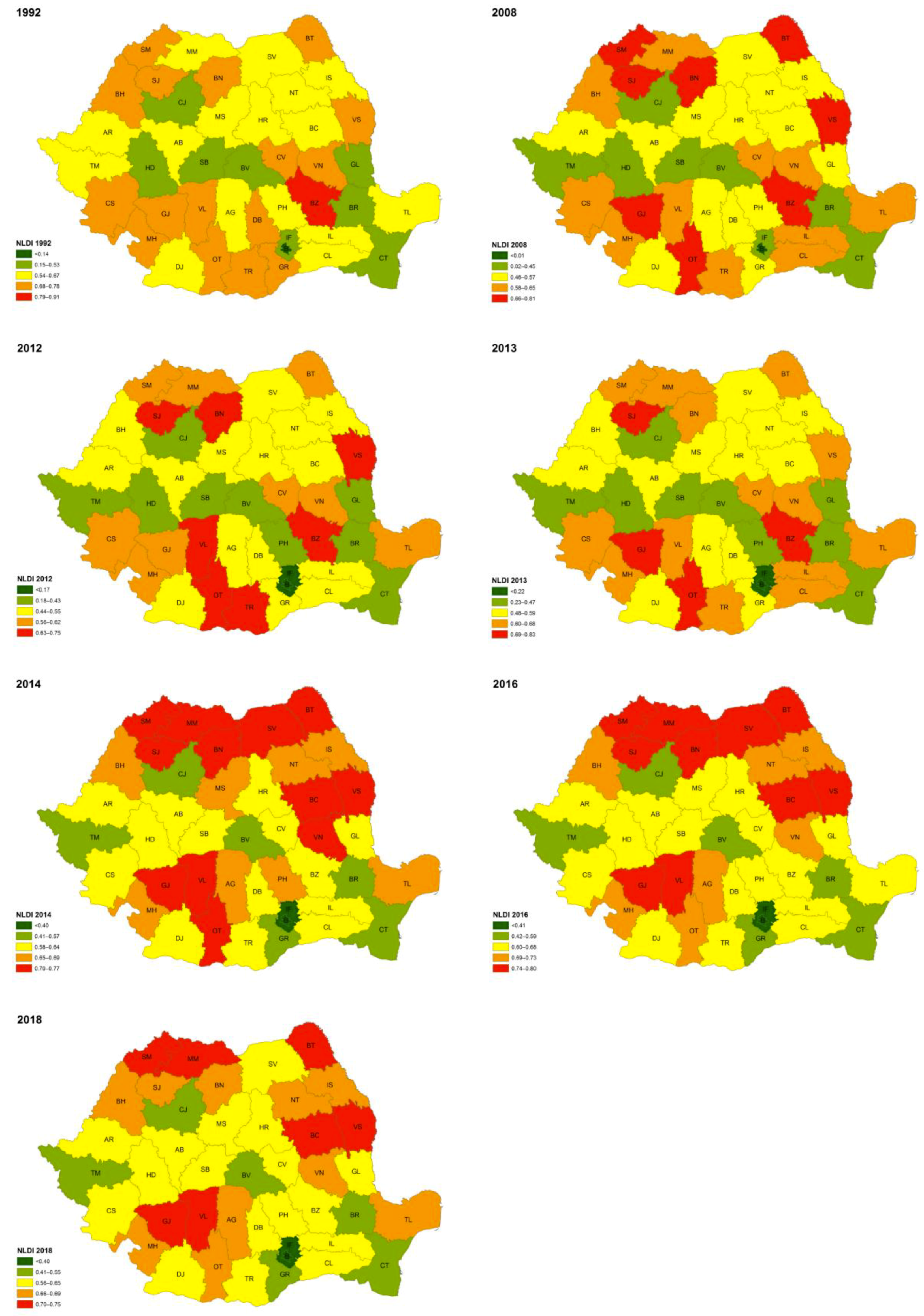
Figures showing the NLDI (Figure 4) illustrate the existing economic development inequalities.
For classification of the NLDI, we used the natural breaks (Jenks) classification method which aims to ensure natural grouping in the data by minimizing variance between classes and maximizing variance across them [33]. The analysis conducted on the NLDI values for each year taken into consideration shows a downward trend until the economic crisis, followed by a short increase. All this illustrates a growing polarization between the most and least developed counties.
Counties with a higher development level and an implicitly lower value of the NLDI are concentrated in the Bucharest capital area, the southern and north-western parts of the historical region of Transylvania (Sibiu (SB), Brașov (BV), Cluj (CJ) counties), and the western border region (Timiș county (TM)) along with areas close to the Black Sea Coast (Constanta county (CT)). These counties have the highest level of human capital and foreign direct investments, and the best accessibility and productivity in Romania [35,36,37,38,39,40].
In contrast, the lowest levels of economic development reflected through the NLDI can be found in the northern, eastern, and south-western parts of Romania (Figure 4), which are among the poorest regions of the EU.
Even though the geographical position and proximity are important factors in development, we cannot unambiguously identify a duality of development between the west and the east or the north and the south, the country being similar to a mosaic of rich and poor areas, reflecting high regional inequalities (Table 3).
The spatial distribution of NLDI values are influenced by a number of factors such as socio-economic variables, demographic variables, and geographical factors. The Pearson correlation coefficient was calculated (Table 3) to highlight the relationship between the NLDI and these factors.
The correlation analysis indicates the preservation of the value and the sign of the relationship between the NLDI and the parameters, in all the years subject to analysis. Thus, the relationship is inverse in terms of development indicators, as the NLDI is higher in the counties with a lower local tax income and GDP per capita. Similar results at the subnational scale in China were obtained by Xu [56] and Zhou [54] using VIIRS night-time radiance. In the case of demographic variables, the NLDI has an indirect relationship with the county population and the positive net migration rate, and a direct relationship with negative net migration rate. There is nothing unusual in these findings: higher levels of economic development are generally related to the positive market effects generated by a larger population concentration. These areas are also attractive for migration due to the higher number of jobs, higher wages, and good quality of life. All these generate positive migration balances. The relationship between the NLDI and the geographical factors indicates higher NLDI values in the counties with a higher average altitude, and an increase of the NLDI values from south to north and from east to west. However, the very low correlation values show that there is no spatial clustering for these parameters (Figure 4).
The results show statistically significant correlations with the variables that reflect the development level and the demographic variables, and non-significant correlations with the geographical variables; except for 2014 and 2016, where we can see a statistically significant direct relationship with latitude. A possible explanation would be the different resolution of the satellite images (VIIRS compared to DMSP), but also an increase of economic development between the north and the south especially after the economic crisis (Figure 4). The relatively small correlation value (0.47) indicates that there is not a very clear differentiation of the development level in the north-south direction, due to the presence of less developed areas in the southwestern part of the country.
Given the low values of the Pearson correlation coefficients for the geographical factors, we further analyzed their relative contribution to the estimation of the NLDI using multiple linear regression. The regression was calculated for the most recent year (2016) for which there is complete data (Table 4). Multiple regression analysis explains ≈80% of the total variability (adjusted R2 = 0.798) of the NLDI for the year under study.
A clearer picture of the results of multiple regression is provided by the relative contribution of each predictor to the total variation explained. The analysis of the standardized coefficients shows a relatively balanced relationship between the socio-economic variables and the demographic variables in the multiple regression results (Table 4). In general, geographical variables had a smaller contribution to the result of the multiple regression, indicating a lower impact on the NLDI values. It should be noted that the income and GDP variables have a greater impact in the calculation of the index than population and net migration rate.
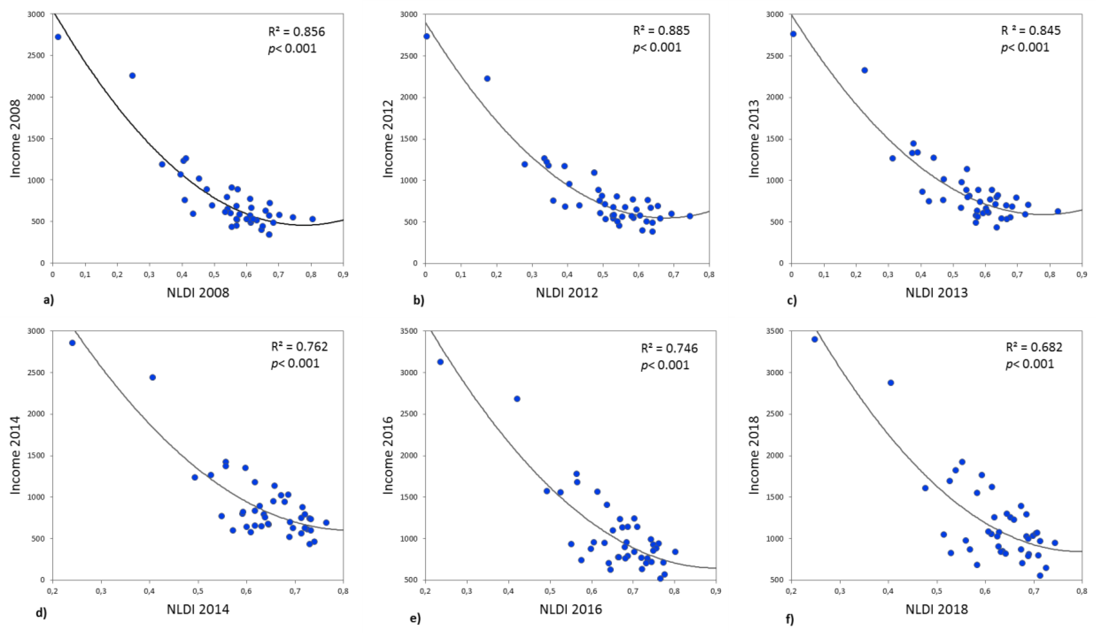
Table 3 shows that the NLDI correlates best with income, which indicates a high potential of the index in estimating income at the county level. In this context, we performed a regression analysis to identify which type of regression was best suited for income estimation. The analysis was conducted only for the 2008–2018 period because there was no income data for 1992. In this analysis we used several criteria to select the best model: total variation explained (R2), error (RMSE), and AIC (Table 5).
The best results were obtained in the second-order (k = 2) polynomial model (Figure 5), for all the criteria considered (Figure 5a–f). The differences are small between the polynomial model and the exponential one, but if we consider R2, we can see a significant improvement compared to the linear model. If we use this model, we can see an improvement of the explained variation by 6% in 2016 and 14% in 2012, compared to linear regression. Similar results were obtained by Dai [12] who, at the provincial scale, highlighted a higher accuracy of the polynomial model compared to the linear one.
Satellite images proved to be a good proxy in estimating economic output and regional inequalities at the subnational level.
One of the main limitations of this study is the statistically insignificant relationship between the NLDI and the income for all 3181 LAU1 (local administrative units: communes and cities). It indicates a low potential of the index in estimating income and measuring inequality at the local level. This may result from the huge differences in population size among LAUs. Therefore, in line with the existing literature, our future research intends to find out the population thresholds where the relationship between the SOL (sum of lights) and income becomes statistically significant.
The second limitation is related to the absence of population data at LAU2 level (villages and towns) for each year. The existence of this data would have helped the authors to improve the NLDI for each year. We will continue to improve our future research by including other datasets such as the annual human settlements or population-grid dataset.
The third important limitation is due to the heterogeneity in the resolution of the satellite images used in the study. Until 2013 we employed lower resolution satellite images (1 kmp), while for the rest of the 2014–2018 period we used higher resolution satellite images (500 kmp). It is hard to overcome this limitation due to the unavailability of higher resolution images before 2013.

5. Conclusions

We demonstrated in our study that Earth observation solutions could play an important role in monitoring progress in the direction of SDG 10 (reduced inequalities). The NLDI calculated from night-time lights (NTL) satellite images proved to be a good proxy for the real time measuring of economic output, while the NLII calculated for the estimation of regional inequalities represents, to our knowledge, an absolute novum in inequality literature. The NLDI has high potential for estimating income and implicitly GDP, as evidenced by the high correlation coefficients. In this regard, the second-order polynomial model proved to be the best model in estimating income, compared to the linear and exponential regression model. The polynomial regression model brings about a significant improvement in the explained variation compared to linear regression.
Moreover, we successfully combined geospatial information and EO (from satellite) with modern data processing (MATLAB, GIS), thus offering an unprecedented opportunity for the real-time tracking of SDG 10. All these tools provided reliable information on the state of economic output and economic regional inequalities, as well as their change over time. We believe that this combination can be successfully used in other spatial and national contexts where data on local tax incomes are available. The above-mentioned combination of methods and techniques is not place-bounded since satellite images are available for all countries. It would be very interesting to see if the relationship between regional economic development and the night-light satellite images is maintained in countries with advanced economies and where light pollution is reduced by modern technologies. Our future research will continue into this direction.
The analysis of the statistical relationship between the NLDI and demographic and socio-economic variables has shown a strong indirect relationship between the NLDI and local tax income and GDP per capita. The lack of relationship between the NLDI and geographical variables shows an aleatory spatial distribution of rich and poor areas. Multiple regression analysis using standardized coefficient values reinforces previous results, with income and GDP having the largest contribution in explaining the total variation.

Author Contributions

All authors contributed equally to the research presented in this paper and to the preparation of the final manuscript. All authors have read and agreed to the published version of the manuscript.

Funding

This work was supported by a grant of Ministery of Research and Innovation, CNCS-UEFISCDI, project number PN-III-P4-ID-PCCF-2016-0084, within PNCDI III.

Acknowledgments

Thanks for the funding support.

Conflicts of Interest

The authors declare no conflicts of interest.

References

  1. United Nations. Sustainable Development Goals. Department of Economic and Social Affairs. Available online: https://sustainabledevelopment.un.org/sdgs (accessed on 12 July 2019).
  2. Mellander, C.; Lobo, J.; Stolarick, K.; Matheson, Z. Night-Time Light Data: A Good Proxy Measure for Economic Activity? PLoS ONE 2015, 10, e0139779. [Google Scholar] [CrossRef] [PubMed] [Green Version]
  3. Benedek, J.; Ivan, K. Remote sensing based assessment of variation of spatial disparities. Geogr. Tech. 2018, 13, 1–9. [Google Scholar] [CrossRef]
  4. Czaran, L. Geospatial and Space Solutions for Monitoring the Sustainable Development Goals (SDGs) and other Global Agendas. Presentation at the CEU Summer School 2019. Available online: https://sunlearning.ceu.edu/pluginfile.php/34895/mod_resource/content/1/Lorant%20Czaran%20%28UNFPA%29%20%20Geospatial%20and%20Space%20Solutions%20for%20monitoring%20the%20Sustainable%20Development%20Goals%20%28SDGs%29%20and%20other%20Global%20Agendas.pdf (accessed on 15 September 2019).
  5. Goldblatt, R.; Heilmann, K.; Vaizman, Y. Can Medium-Resolution Satellite Imagery Measure Economic Activity at Small Geographies? Evidence from Landsat in Vietnam. World Bank Econ. Rev. 2019, lhz001, 1–19. [Google Scholar] [CrossRef]
  6. Kang, M.; Jung, M.C. Night on South Korea: Unraveling the Relationship between Urban Development Patterns and DMSP-OLS Night-Time Lights. Remote Sens. 2019, 11, 2140. [Google Scholar] [CrossRef] [Green Version]
  7. Taubenböck, H.; Dahle, F.; Geiß, C.; Wurm, M. Europe’s Socio-Economic Disparities Reflected in Settlement Patterns Derived from Satellite Data; Joint Urban Remote Sensing Event (JURSE): Vannes, France, 2019; pp. 1–4. [Google Scholar] [CrossRef]
  8. Ebener, S.; Murray, C.; Tandon, A.; Elvidge, C. From wealth to health: Modeling the distribution of income per capita at the sub-national level using nighttime lights imagery. Int. J. Health Geogr. 2005, 4, 5–11. [Google Scholar] [CrossRef] [Green Version]
  9. Ghosh, T.; Powell, R.L.; Elvidge, C.D.; Baugh, K.E.; Sutton, P.C.; Anderson, S. Shedding Light on the Global Distribution of Economic Activity. Open Geogr. J. 2010, 3, 148–161. [Google Scholar] [CrossRef]
  10. Basihos, S. Nightlights as a Development Indicator: The Estimation of Gross Provincial Product (GPP) in.Turkey (5 May 2016). Available online: https://ssrn.com/abstract=2885518 (accessed on 19 May 2019).
  11. Bhandari, L.; Roychowdhury, K. Night lights and economic activity in India: A study using DMSP-OLS night time images. Proc. Asia Pac. Adv. Netw. 2011, 32, 218–236. [Google Scholar] [CrossRef]
  12. Dai, Z.; Hu, Y.; Zhao, G. The Suitability of Different Nighttime Light Data for GDP Estimation at Different.Spatial Scales and Regional Levels. Sustainability 2017, 9, 305. [Google Scholar] [CrossRef] [Green Version]
  13. Chen, X.; Nordhaus, W.D. Using luminosity data as a proxy for economic statistics. Proc. Natl. Acad. Sci. USA 2011, 108, 8589–8594. [Google Scholar] [CrossRef] [Green Version]
  14. Li, X.; Ge, L.L.; Chen, X.L. Detecting Zimbabwe’s decadal economic decline using nighttime light imagery. Remote Sens. 2013, 5, 4551–4570. [Google Scholar] [CrossRef] [Green Version]
  15. Li, S.; Zhang, T.; Yang, Z.; Li, X.; Xu, H. Night Time Light Satellite Data for Evaluating the Socioeconomics in Central Asia. Int. Arch. Photogramm. Remote Sens. Spatial Inf. Sci. 2017, XLII–2/W7, 1237–1243. [Google Scholar] [CrossRef] [Green Version]
  16. Elvidge, C.; Zhizhin, M.; Baugh, K.; Hsu, F.-C. Automatic Boat Identification System for VIIRS Low Light Imaging Data. Remote Sens. 2015, 7, 3020–3036. [Google Scholar] [CrossRef] [Green Version]
  17. Bennie, J.; Davies, T.W.; Duffy, J.P.; Inger, R.; Gaston, K.J. Contrasting trends in light pollution across Europe based on satellite observed night time lights. Sci. Rep. 2014, 4, 3789. [Google Scholar] [CrossRef] [PubMed] [Green Version]
  18. Bennie, J.; Duffy, J.P.; Davies, T.W.; Correa-Cano, M.E.; Gaston, K.J. Global trends in exposure to light pollution in natural terrestrial ecosystems. Remote Sens. 2015, 7, 2715–2730. [Google Scholar] [CrossRef] [Green Version]
  19. Jiang, W.; He, G.J.; Long, T.F.; Wang, C.; Ni, Y.; Ma, R.Q. Assessing light pollution in china based on nighttime light imagery. Remote Sens. 2017, 9, 135. [Google Scholar] [CrossRef] [Green Version]
  20. Small, C.; Pozzi, F.; Elvidge, C.D. Spatial analysis of global urban extent from DMSP-OLS night lights. Remote Sens. Environ. 2005, 96, 277–291. [Google Scholar] [CrossRef]
  21. Ma, T.; Zhou, C.; Pei, T.; Haynie, S.; Fan, J. Quantitative estimation of urbanization dynamics using time series of DMSP/OLS nighttime light data: A comparative case study from China’s cities. Remote Sens. Environ. 2012, 124, 99–107. [Google Scholar] [CrossRef]
  22. Liu, Z.; He, C.; Zhang, Q.; Huang, Q.; Yang, Y. Extracting the dynamics of urban expansion in China using DMSP-OLS nighttime light data from 1992 to 2008. Landsc. Urban Plan. 2012, 106, 62–72. [Google Scholar] [CrossRef]
  23. Gao, B.; Huang, Q.; He, C.; Dou, Y. Similarities and differences of city-size distributions in three main urban agglomerations of China from 1992 to 2015: A comparative study based on nighttime light data. J. Geogr. Sci. 2017, 27, 533–545. [Google Scholar] [CrossRef]
  24. Ghosh, T.; Anderson, S.J.; Elvidge, C.D.; Sutton, P.C. Using nighttime satellite imagery as a proxy measure of human well-being. Sustainability 2013, 5, 4988–5019. [Google Scholar] [CrossRef] [Green Version]
  25. Shi, K.; Huang, C.; Yu, B.; Yin, B.; Huang, Y.; Wu, J. Evaluation of NPP-VIIRS night-time light composite data for extracting built-up urban areas. Remote Sens. Lett. 2014, 5, 358–366. [Google Scholar] [CrossRef]
  26. Sharma, R.C.; Tateishi, R.; Hara, K.; Gharechelou, S.; Iizuka, K. Global mapping of urban built-up areas of year 2014 by combining MODIS multispectral data with VIIRS nighttime light data. Int. J. Digit. Earth 2016, 9, 1004–1020. [Google Scholar] [CrossRef]
  27. Kiran Chand, T.R.; Badarinath, K.V.S.; Elvidge, C.D.; Tuttle, B.T. Spatial characterization of electrical power consumption patterns over India using temporal DMSP-OLS night-time satellite data. Int. J. Remote Sens. 2009, 30, 647–661. [Google Scholar] [CrossRef]
  28. He, C.; Ma, Q.; Liu, Z.; Zhang, Q. Modeling the spatiotemporal dynamics of electric power consumption in Mainland China using saturation-corrected DMSP/OLS nighttime stable light data. Int. J. Digit. Earth 2014, 7, 993–1014. [Google Scholar] [CrossRef]
  29. Min, B.; Gaba, K.M.; Sarr, O.F.; Agalassou, A. Detection of rural electrification in Africa using DMSP-OLS night lights imagery. Int. J. Remote Sens. 2013, 34, 8118–8141. [Google Scholar] [CrossRef]
  30. Pandey, B.; Joshi, P.K.; Seto, K.C. Monitoring urbanization dynamics in India using DMSP/OLS nighttime lights and SPOT-VGT data. Int. J. Appl. Earth Obs. 2013, 23, 49–61. [Google Scholar] [CrossRef]
  31. Shi, K.; Chen, Y.; Yu, B.; Xu, T.; Yang, C.; Li, L.; Huang, C.; Chen, Z.; Liu, R.; Wu, J. Detecting spatiotemporal dynamics of global electric power consumption using DMSO/OLS nighttime stable light data. Appl. Energy 2016, 184, 450–463. [Google Scholar] [CrossRef]
  32. Schroeder, W. Visible Infrared Imaging Radiometer Suite (VIIRS) 375 m & 750 m Active Fire Detection Data Sets Based on Nasa VIIRS Land Science Investigator Processing System (SIPS) Reprocessed Data-Version 1. NASA, 2017. Available online: https://lpdaac.usgs.gov/sites/default/files/public/product_documentation/vnp14_user_guide_v1.3.pdf (accessed on 17 June 2019).
  33. Nagy, J.A.; Benedek, J.; Ivan, K. Measuring Sustainable Development Goals at a Local Level: A Case of a. Metropolitan Area in Romania. Sustainability 2018, 10, 3962. [Google Scholar] [CrossRef] [Green Version]
  34. Zaman, G.; Goschin, Z. Economic Crisis and Wage Divergence: Empirical Evidence from Romania. Prague Econ. Pap. 2014, 4, 493–513. [Google Scholar] [CrossRef]
  35. Moroianu, N.D.; Constantin, D.L.; Herteliu, C.; Novac, A. Empirical Weighted Modelling on Inter-County Inequalities Evolution and to Test Economical Convergence in Romania. USV Ann. Econ. Public Adm. 2015, 15, 150–180. [Google Scholar]
  36. Moisescu, E.R. Regional convergence. Case of Romania. Theor. Appl. Econ. 2015, 2, 183–188. [Google Scholar]
  37. Török, I. From growth to shrinkage: The effects of economic change on the migration processes in rural Romania. Landbauforshung 2014, 64, 195–206. [Google Scholar] [CrossRef]
  38. Benedek, J. Spatial differentiation and core-periphery structures in Romania. East. J. Eur. Stud. 2015, 6, 49–61. [Google Scholar]
  39. Oancea, B.; Andrei, T.; Pirjol, D. Income distribution in Romania: The exponential-Pareto distribution. Phys. A Stat. Mech. Appl. 2017, 469, 486–498. [Google Scholar] [CrossRef]
  40. Benedek, J.; Lembcke, A.C. Characteristics of recovery and resilience in the Romanian regions. East. J. Eur. Stud. 2017, 8, 95–126. [Google Scholar]
  41. Benedek, J.; Cristea, M.; Szendi, D. Catching up or falling behind? Economic convergence and regional development trajectories in Romania. Rom. Rev. Reg. Stud. 2015, 11, 15–34. [Google Scholar]
  42. Goschin, Z. Exploring regional economic convergence in Romania. A spatial modeling approach. East. J. Eur. Stud. 2017, 2, 127–146. [Google Scholar]
  43. Török, I.; Benedek, J. Spatial patterns of local income inequalities. J. Settl. Spat. Plan. 2018, 2, 77–91. [Google Scholar] [CrossRef]
  44. Pinkovskiy, M.; Sala-i-Martin, X. Lights, camera. income! Illuminating the national accounts-household surveys debate. Q. J. Econ. 2016, 131, 579–631. [Google Scholar] [CrossRef]
  45. Tselios, V. Growth and convergence in income per capita and income inequality in the regions of the EU. Spat. Econ. Anal. 2009, 4, 343–370. [Google Scholar] [CrossRef]
  46. Rey, S.J.; Sastré-Gutiérrez, M.L. Interregional inequality dynamics in Mexico. Spat. Econ. Anal. 2010, 5, 277–298. [Google Scholar] [CrossRef]
  47. Paredes, D. The role of human capital, market potential and natural amenities in understanding spatial wage disparities in Chile. Spat. Econ. Anal. 2013, 8, 154–175. [Google Scholar] [CrossRef]
  48. Sacchi, A.; Salotti, S. The effects of fiscal decentralization on household income inequality: Some empirical evidence. Spat. Econ. Anal. 2014, 9, 202–222. [Google Scholar] [CrossRef]
  49. De Dominicis, L. Inequality and growth in European regions: Towards a place-based approach. Spat. Econ. Anal. 2014, 9, 120–141. [Google Scholar] [CrossRef]
  50. Ezcurra, R.; Rodríguez-Pose, A. Trade openness and spatial inequality in emerging countries. Spat. Econ. Anal. 2014, 9, 162–182. [Google Scholar] [CrossRef]
  51. Monastiriotis, V. Regional growth and national development: Transition in Central and Eastern Europe and the regional Kuznets curve in the east and the west. Spat. Econ. Anal. 2014, 9, 142–161. [Google Scholar] [CrossRef] [Green Version]
  52. Pereira, J.; Galego, A. Intra-regional wage inequality in Portugal. Spat. Econ. Anal. 2015, 10, 79–101. [Google Scholar] [CrossRef] [Green Version]
  53. Gluschenko, K. Measuring regional inequality: To weight or not to weight? Spat. Econ. Anal. 2018, 13, 36–59. [Google Scholar] [CrossRef]
  54. Zhou, Y.; Ma, T.; Zhou, C.; Xu, T. Nighttime light derived assessment of regional inequality of socioeconomic development in China. Remote Sens. 2015, 7, 1242–1262. [Google Scholar] [CrossRef] [Green Version]
  55. Elvidge, C.D.; Baugh, K.E.; Anderson, S.J.; Sutton, P.C.; Ghosh, T. The Night Light Development Index (NLDI): A spatially explicit measure of human development from satellite data. Soc. Geogr. 2012, 7, 23–35. [Google Scholar] [CrossRef]
  56. Xu, H.; Yang, H.; Li, X.; Jin, H.; Li, D. Multi-Scale Measurement of Regional Inequality in Mainland China during 2005–2010 using DMSP/OLS Night Light Imagery and Population Density Grid Data. Sustainability 2015, 7, 13469–13499. [Google Scholar] [CrossRef] [Green Version]
  57. Li, X.; Li, D.; Xu, H.; Wu, C. Intercalibration between dmsp/ols and viirs night-time light images to evaluate city light dynamics of syria’s major human settlement during syrian civil war. Int. J. Remote Sens. 2017, 38, 1–18. [Google Scholar] [CrossRef]
  58. Salvati, L.; Guandalini, A.; Carlucci, M.; Chelli, M.F. An empirical assessment of human development through remote sensing: Evidences from Italy. Ecol. Indic. 2017, 78, 167–172. [Google Scholar] [CrossRef]
  59. Wu, R.; Yang, D.; Dong, J.; Zhang, L.; Xia, F. Regional inequality in China based on NPP-VIIRS night-time light imagery. Remote Sens. 2018, 10, 240. [Google Scholar] [CrossRef] [Green Version]
  60. Version 4 DMSP-OLS Nighttime Lights Time Series. NOAA/NGDC Database. Available online: https://ngdc.noaa.gov/eog/dmsp/downloadV4composites.html (accessed on 28 March 2019).
  61. Version 1 VIIRS Day/Night Band Nighttime Lights. The Earth Observations Group (EOG). Available online: https://eogdata.mines.edu/download_dnb_composites.html (accessed on 1 March 2019).
  62. National Institute of Statistics of Romania. Population and Dwellings Census. Available online: http://www.recensamantromania.ro (accessed on 15 March 2018).
  63. National Institute of Statistics. Bucharest, Romania. Available online: http://www.insse.ro (accessed on 21 March 2019).
  64. Eurostat Database. Available online: http://ec.europa.eu/eurostat/ (accessed on 21 March 2019).
  65. Ministry of Regional Development and Public Administration (MRDPA). Bucharest, Romania. Available online: https://www.mdrap.ro/en/ (accessed on 17 June 2019).
  66. Benedek, J.; Varvari, Ș.; Litan, C. Urban growth pole policy and regional development: Old vine in new bottles. In Regional and Local Development in Times of Polarization. Re-Thinking Spatial Policies in Europe; Lang, T., Görmar, F., Eds.; Palgrave/MacMillan: Basingstoke, UK, 2019; pp. 173–196. [Google Scholar]
  67. Rodríguez-Pose, A.; Tselios, V. Toward inclusive growth: Is there regional convergence in social welfare? Int. Reg. Sci. Rev. 2015, 38, 30–60. [Google Scholar] [CrossRef]
  68. Lengwiler, Y. Computes the Gini Coefficient and the Lorentz Curve of Weighted Data. Available online: https://nl.mathworks.com/matlabcentral/fileexchange/28080-gini-coefficient-and-the-lorentz-curve (accessed on 17 March 2019).
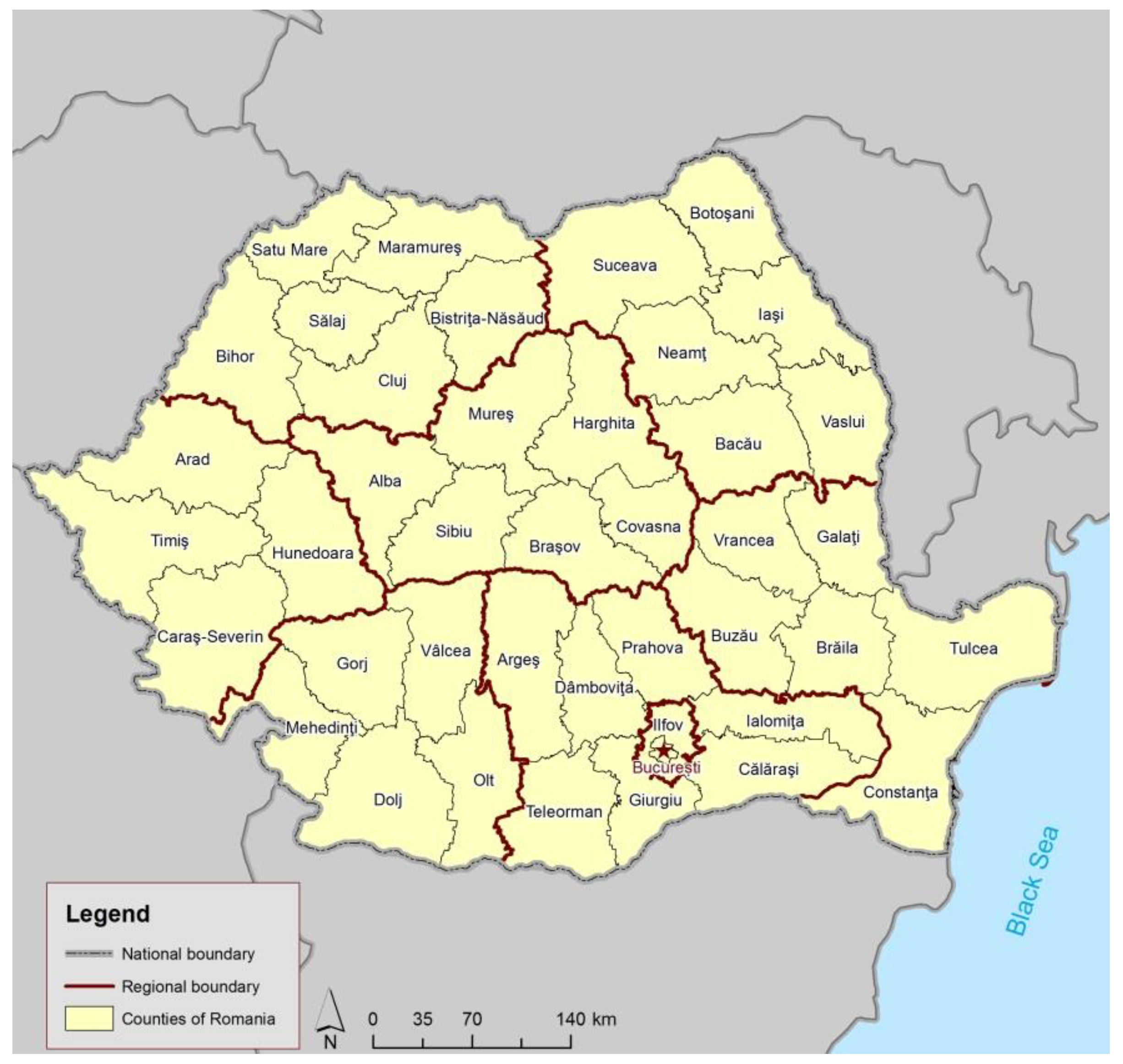
Figure 1. Administrative organization of Romania.
Remotesensing 12 00033 g001
Figure 2. Spatial distribution of night-time light in Romania, 1992 and 2018.
Remotesensing 12 00033 g002
Figure 3. Graphical representation of the Lorenz curve.
Remotesensing 12 00033 g003
Figure 4. Night Light Development Index at the county level, 1992–2018.
Remotesensing 12 00033 g004
Figure 5. Polynomial model between NLDI and income, a-f 2008–2018.
Remotesensing 12 00033 g005
Table 1. Description of the data used in this study.
DataData DescriptionYear
DMSP-OLS NTLannual product–stable light composite1992, 2008, 2012, 2013
DMSP-OLS NTLannual product–average light composite1992, 2008, 2012, 2013
NPP-VIIRS DNBannual product–“vcm-orm-ntl”2016
NPP-VIIRS DNBmonthly product–“vcmslcfg”2014, 2018
(April, May, June, July, August, September)
Table 2. Data descriptives. GDP, gross domestic product.
MeanStandard Deviation
GDP per capitaLocal tax incomeNet migration ratePopulation GDP per capitaLocal tax incomeNet migration ratePopulation
1992**−2.0550,6381992**3.4309,804.9
200810,935.7751.1−0.2536,718.320084887.1457.95.4308,976.7
201212,173.8802.7−0.4533,377.720125102.5447.95.8308,994.3
201312,226.2883.1−0.5532,377.420135278451.75.7308,117.2
201412,690.5908.9−0.4530,94620145585.5469.86.1304,972.3
201614,540.51068.2−1.0529,43020166363.7520.26.5305,148
2018*1200.8−1.8528,038.22018*554.55.7309,051.3
MinimumMaximum
GDP per capitaLocal tax incomeNet migration ratePopulation GDP per capitaLocal tax incomeNet migration ratePopulation
1992**−9.4235,1961992**6.92,191,176
20085900340.4−5.8232,279200833,000272431.42,158,816
20127000389.0−6.1230,600201236,4002739.734.42,151,758
20136800438.9−7.0230,226201337,7002768.531.82,140,816
20147000436.4−4.9229,563201439,4002861.535.22,110,752
20168100519.3−6.4228,492201645,6003131.237.72,102,675
2018*559.3−10.3226,8792018*3402.629.12,121,794
Table 3. Pearson correlation coefficient between Night Light Development Index (NLDI) and analyzed variables.
YearAltitudeX_LongY_LatLocal Tax IncomeGDP /Capita Positive Net Migration RateNegative Net Migration RatePopulation
19920.105−0.1620.120**−0.747 *−0.131−0.277−0.669 *
20080.088−0.0850.247−0.864 *−0.840 *−0.743 *−0.044−0.666 *
20120.102−0.0550.222−0.862 *−0.840 *−0.748 *0.308−0.637 *
20130.093−0.0770.170−0.858 *−0.824 *−0.560 *0.306−0.670 *
20140.288−0.1200.470 *−0.827 *−0.797 *−0.689 *0.205−0.553 *
20160.304−0.1180.474 *−0.831 *−0.806 *−0.741 *0.110−0.573 *
* Significant correlations; ** no data.
Table 4. Regression coefficients.
YearVariableUnstandardized CoefficientsStandardized Coefficients
2016(Constant)0.783
GDP per capita−0.00000755−0.450
Altitude0.000050780.127
X_Long−0.00000009−0.121
Y_Lat0.000000230.273
Local tax income−0.00008564−0.418
Net migration rate−0.00000516−0.384
Population−0.00000011−0.311
Table 5. Income fitting precision values based on NLDI at county level.
ModelMetric 1200820122013201420162018
LinearR20.7460.7430.7360.6830.6910.617
Adjusted R20.7400.7370.7290.6750.6830.607
RMSE233,512229,753235,001267,680292,820347,545
AIC460,022458,659460,556471,493479,034493,426
PolynomialR20.8560.8850.8450.7620.7460.682
RMSE178,054155,534182,044235,052268,758320,801
AIC440,183428,824442,044463,511474,768489,636
ExponentialR20.8390.8700.8290.7520.7390.677
RMSE188,374165,788191,394239,688272,340323,133
AIC444,915434,187446,252465,152475,880490,245
1 Abbreviations: RMSE, root square mean error; AIC, Akaike information criterion.