Article

Comparing Deep Learning and Shallow Learning for Large-Scale Wetland Classification in Alberta, Canada

1
Alberta Biodiversity Monitoring Institute, University of Alberta, Edmonton, AB T6G 2E9, Canada
2
Independent Researcher, Revelstoke, BC 2773, Canada
3
C-CORE and Department of Electrical Engineering, Memorial University of Newfoundland, St. John’s, NL A1B 3X5, Canada
4
Canada Centre for Mapping and Earth Observation, Natural Resources Canada, 560 Rochester Street, Ottawa, ON K1A 0Y7, Canada
5
Alberta Environment and Parks, Government of Alberta, 200 5 Ave S, Lethbridge, AB T1J 4L1, Canada
*
Author to whom correspondence should be addressed.
Remote Sens. 2020, 12(1), 2; https://doi.org/10.3390/rs12010002
Submission received: 31 October 2019 / Revised: 9 December 2019 / Accepted: 11 December 2019 / Published: 18 December 2019
(This article belongs to the Special Issue Wetland Landscape Change Mapping Using Remote Sensing)

Abstract

:
Advances in machine learning have changed many fields of study and it has also drawn attention in a variety of remote sensing applications. In particular, deep convolutional neural networks (CNNs) have proven very useful in fields such as image recognition; however, the use of CNNs in large-scale remote sensing landcover classifications still needs further investigation. We set out to test CNN-based landcover classification against a more conventional XGBoost shallow learning algorithm for mapping a notoriously difficult group of landcover classes, wetland class as defined by the Canadian Wetland Classification System. We developed two wetland inventory style products for a large (397,958 km2) area in the Boreal Forest region of Alberta, Canada, using Sentinel-1, Sentinel-2, and ALOS DEM data acquired in Google Earth Engine. We then tested the accuracy of these two products against three validation data sets (two photo-interpreted and one field). The CNN-generated wetland product proved to be more accurate than the shallow learning XGBoost wetland product by 5%. The overall accuracy of the CNN product was 80.2% with a mean F1-score of 0.58. We believe that CNNs are better able to capture natural complexities within wetland classes, and thus may be very useful for complex landcover classifications. Overall, this CNN framework shows great promise for generating large-scale wetland inventory data and may prove useful for other landcover mapping applications.

Graphical Abstract

1. Introduction

Machine learning—a method where a computer discovers rules to execute a data processing task, given training examples—can generally be divided into two categories: Shallow learning and deep learning methods [1]. Deep learning uses many successive layered representations of data (i.e., hundreds of convolutions/filters), while shallow learning typically uses one or two layered representations of the data [1]. Deep learning has shown great promise for tackling many tasks such as image recognition, natural language processing, speech recognition, superhuman Go playing, and autonomous driving [1,2,3].
In remote sensing, shallow learning for landcover classification is a well-established method. Countless studies have used random forest [4], support vector machine (SVM) [5], boosted regression trees [6,7], and many other algorithms to classify landcover from Earth observation and remote sensing data. These algorithms typically work on a pixel-level or object-level. Pixel-level algorithms extract the numerical value of the remote sensing inputs (i.e., vegetation index value, radar backscatter, relative elevation) and match that to a known landcover class (i.e., forest). With this numerical data, a shallow learning model can be built through methods such as kernel methods/decision boundaries [8], decision trees [9], and gradient boosting [10]. These models can then be used to predict the landcover class of an unknown pixel with a unique numerical representation. In a somewhat different fashion, object-based shallow learning methods use features, such as texture, edge detection, and contextual information [11,12], of a given area to classify landcover. Once segmented (using k-Nearest-Neightbours, spectral clustering, etc.), these object-based algorithms often use similar shallow learning techniques to predict a given landcover class [13]. Both pixel- and object-based methods are widely used and both have their pros and cons [12].
The use of deep learning in remote sensing is a more recent development and it is gaining popularity [14,15,16,17,18]. Of the many types of deep learning approaches that exist, we have selected a segmentation convolutional neural network (CNN) method. In the literature, there are two commonly used CNN models for landcover classification [17]: Patch-based CNNs [19] and fully convolutional networks (FCNs) [20]. In the patch-based CNNs, a remote sensing scene is divided into several patches and a typical CNN model is applied to predict a single label for the center of each patch. On the other hand, in FCN models, the fully connected layers are replaced with convolutional layers. Therefore, FCNs can maintain a two-dimensional output image structure and this increases its training efficiency. Typically, CNN architectures can incorporate multiple stacked layers as inputs, which can be from different sources (i.e., optical and synthetic aperture radar (SAR) sensors) [21]. These training patches then undergo a series of filters/convolutions/poolings to extract hierarchical features from the data, such as low-level edge and curved features, along with higher level textural or unique spectral features. Our specific segmentation CNN architecture used in this study is known as a U-Net style [22].
In this study, we focus on the prediction of wetland class (bog, fen, marsh, and swamp), as defined by the Canadian Wetland Classification System [23], and the prediction of upland and open water classes to fill out the classified map. Uses of spatially-explicit wetland inventories have become even more imperative lately due to their increased applications for carbon pricing, ecosystem services, and biodiversity conservation efforts [24,25,26]. Wetlands store a much higher relative percentage of soil carbon when compared to other vegetated habitats such as forest or agriculture [24]. They are vital for hydrological services, such as flood remediation and filtering of freshwater [26]. Wetland carbon and hydrological processes are also both important in the context of climate change, as wetlands have the ability to store or release vast amounts of carbon [27,28] and may be able to mitigate changes to hydrology caused by variations in precipitation [29]. These represent some of the reasons why the Government of Alberta seeks to update the current provincial wetland inventory, the Alberta Merged Wetland Inventory [30], to yield a consistent baseline state of the environment product, which can be leveraged for monitoring and reporting purposes, and to aid policy-makers in the strategic management of wetlands. The update will follow the Canadian Wetland Classification System (CWCS) wetland classes, whilst simultaneously conforming to defined minimum mapping unit and classification accuracy criteria. The machine learning methods investigated in the current study demonstrate high relevance in the creation of such a product.
Spatial wetland inventories such as the Alberta Merged Wetland Inventory need to consider the class of wetland, because certain wetland classes are more sensitive to certain types of disturbance. For example, fens—peatlands with flowing water—are very sensitive to anthropogenic pressure, i.e., new roads and linear features acting like dams to moving water [31]. Bogs—peatlands with stagnant water—are more sensitive to climate-driven changes in precipitation patterns because bogs are recharged through precipitation [32]. Marshes and swamps are also sensitive to climate change due to their reliance on predictable seasonal flooding cycles [33].
Spatial wetland inventories at a country or provincial scale [30,31,32,33,34] are not new, but having data that are reliable for land management and land planning decisions is a challenge. In Canada, mapping of wetlands via remote sensing is a well-studied topic [35]. Initially, inventories were typically built through aerial image interpretation [36]. While accurate, this methodology is usually very time consuming and costly. Given Canada’s commitment to, and involvement with, synthetic aperture radar (SAR) data, many studies have used SAR to map and monitor wetlands [37,38,39,40,41,42,43,44,45] with varying degrees of success. It appears SAR data are most useful for monitoring the dynamics of wetlands. Other studies and projects have used moderate resolution optical data such as Landsat or Sentinel-2 to generate wetland inventories [30,46,47]. Most modern approaches to large-scale wetland inventories utilize a fusion of data such as SAR and optical [34,39,48] and, ideally, SAR, optical, plus topographic information [6,7,49]. Theoretically the fusion of SAR, optical, and topographic information should give the most information on wetlands and wetland class because: (1) SAR is sensitive to the physical structure of vegetation and can detect the dynamic nature of wetlands with a rich time series stack; (2) optical data can capture variations in vegetation type and vegetation productivity, as it is sensitive to the molecular structure of vegetation; and (3) topographic information can provide data about hydrological patterns which drive wetland formation and function.
It is our understanding that all of the machine learning studies listed in the paragraph above used shallow learning methods, such as random forest, SVM, or boosted regression trees. It appears that distinguishing wetland class with remote sensing data and shallow machine learning is still a difficult task. This is likely due to the fact that one wetland class (i.e., fen) can have different vegetation types—forested, shrubby, graminoid [35]. Additionally, wetlands of different classes can have identical vegetation and vegetation structure. These types are then only distinguished through their below-ground hydrological patterns. Finally, wetland classes do not have a defined boundary, since they gradually transition into another class or upland habitat [
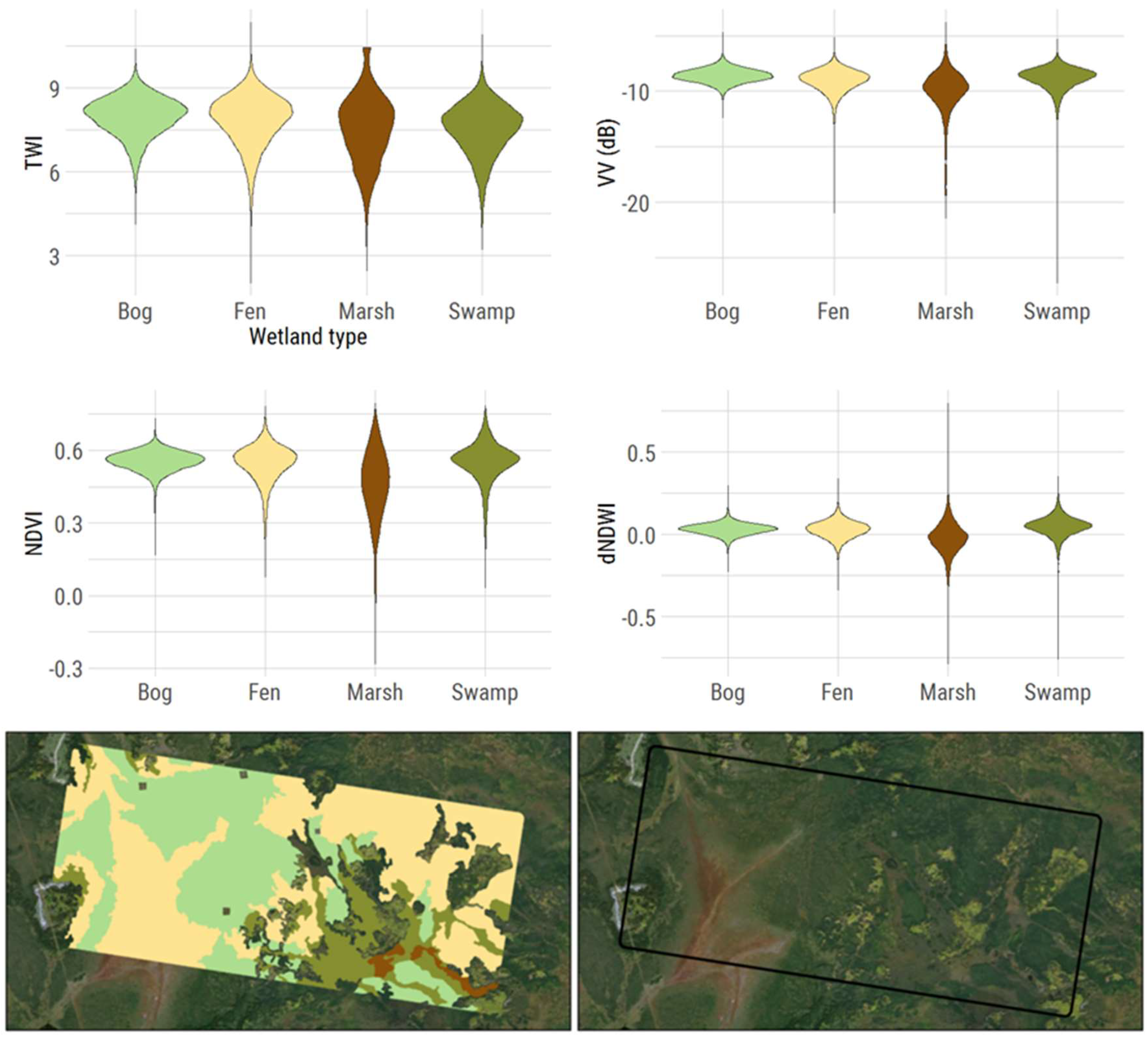
50]. This makes spatially explicit inventories inherently inaccurate because a hard boundary must be identified. These issues with wetland and wetland class mapping are best summed up in Figure 1. Given three different data sources (SAR, optical, and topographic) with static and multi-temporal remote sensing measures, the four wetland classes do not show any noticeable differences on a pixel level (top panel of Figure 1). The violin plots show the distribution of numerical values for all four wetland classes (essentially a vertical histogram by class). Marshes may show a wider distribution of values, but fens, bogs, and swamps are almost identical. In the bottom panel of Figure 1, even the visual identification of these wetland classes with high resolution imagery is difficult. Fens, in the bottom right of the image, can be seen visually (flow lines and lighter tan color), but then fens appear very different in the top right corner (dark green color and appear to be treed).
With the known difficulty of wetland classification with shallow learning (Figure 1), we believe wetland class mapping is the perfect candidate for deep learning and CNNs. In practice, CNNs trained on a patch-level learn low- and high-level features from the remote sensing data. For example, waterline edges which delineate marshes and open water may only need simple edge detection convolution filters, while fens and bogs may be differentiated by subtle variations in texture or color (i.e., visible flow lines in fens). Within the last couple of years, a number of studies have attempted to use deep learning for wetland mapping in Canada over small areas and have achieved promising results when compared to alternative shallow learning methods [20,51,52].
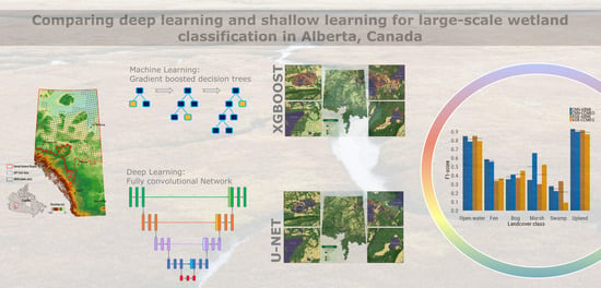
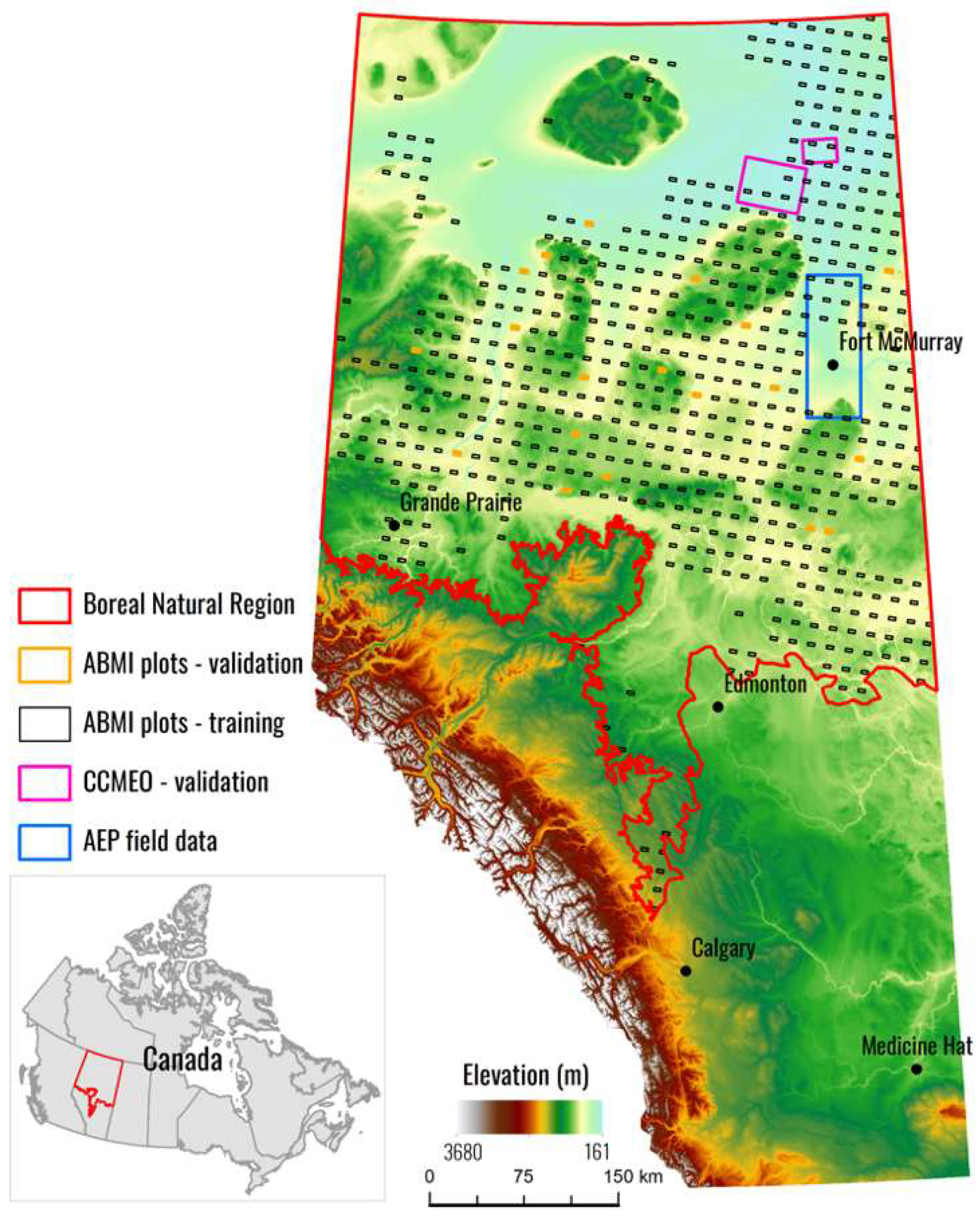
With the current status of machine learning and the history of Canadian wetland mapping in mind, we propose a simple goal for this study: To compare deep learning (CNN) classifications with shallow learning (XGBoost) classifications for wetland class mapping over a large region of Alberta, Canada (397,958 km2) using the most up-to-date, open source, fusion of data sources from Sentinel-1 (SAR), Sentinel-2 (optical), and the Advanced Land Observing Satellite (ALOS) digital elevation model (DEM) (topographic). To reach a strong conclusion, we plan to validate our results against three validation data sets: Two generated from photo interpretation and one field validation data set. These results will guide future large-scale spatial wetland inventory efforts in Canada. If deep learning techniques are found to generate better products, new wetland inventories projects should adopt deep learning workflows. If shallow learning methods still produce comparable results, they should continue to be used in wetland inventory workflow; however, deep learning architectures should still remain an active area of research with regard to methods for wetland mapping.

2. Methods

2.1. Study Area

Our study area includes the Boreal Natural Region (BNR) of Alberta, Canada, along with parts of the Canadian Shield, Parkland, and Foothills Natural Regions (Figure 2). The study area comprises 60% (397,958 km2) of the total area of Alberta. Elevations range from 150 m above sea level in the northeast to 1100 m near the Alberta–British Columbia border [53].
The BNR has short summers and long, cold winters [53]. Vegetation consists of vast deciduous, mixed wood, and coniferous forests interspersed with large wetland complexes [53]. Agriculture is limited to the southeast region of the study area (northeast of Edmonton, a large urban center) and areas around Grand Prairie (western portion of the study area) [54]. Other anthropogenic features are from forestry activities and extensive oil and gas development in the regions around Fort McMurray [55].
The Alberta Wetland Classification System recognizes five main wetland classes across the province: Bog, fen, marsh, swamp, and shallow open water [30,31,32,33,34,35,36,37,38,39,40,41,42,43,44,45,46,47,48,49,50,51,52,53,54,55]. The BNR is dominated by fens and bogs (peatlands), which typically form in cool, flat, low-lying areas with poorly drained soils and peat accumulations of 30–40 cm or more [56,57]. The fens and bogs of this region are classified as wooded coniferous, shrubby, or graminoid, with bogs being relatively acidic and fens ranging from poor acidic to extreme-rich alkaline [55,56,57,58]. Fens and bogs are typically differentiated by their hydrology. Fens are fed by flowing ground water and precipitation, while bogs are fed solely by precipitation and have relatively stagnant water. Marshes are periodically inundated areas consisting mainly of emergent graminoid vegetation, while swamps are typically forested or shrubby and have standing water for longer periods of time and vegetation consists of dense conifer or deciduous forests [59].

2.2. Data

Data for these landcover classifications came from three sources: Sentinel-1 SAR, Sentinel-2 optical, and ALOS DEM data. All inputs can be seen in Table 1. All data used in this study were acquired, processed, and downloaded through the Google Earth Engine (GEE) JavaScript API [60]. Each Sentinel-1 ground range-detected image in GEE was pre-processed with the Sentinel-1 toolbox using the following steps: Thermal noise removal, radiometric calibration, and terrain correction using the Shuttle Radar Topography Mission (SRTM) 30 m DEM. All Sentinel-1 dual pol (VV VH) images over Alberta during the spring/summer time period (15 May–15 August) for the years 2017 and 2018 were used. This yielded 1123 Sentinel-1 images. All of these images were then further processed with: An angle correction [61], edge mask for dark strips on the edges of images, and a multi-temporal filtering using a two-month window [62]. To obtain the static backscatter inputs, the mean pixel value of the image stack was calculated. Additionally, the polarization ratio was calculated by dividing the VH polarization by the VV polarization. Sentinel-1 time series metrics were calculated in the same manner, but restricted to certain dates. Delta VH was calculated by subtracting winter backscatter (1 November– 31 March) from summer backscatter (1 June–15 August).
Sentinel-2 top of atmosphere data were acquired over all of Alberta for the same time period as the Sentinel-1 data. Note that Sentinel-2 surface reflectance products were not available in GEE at the start of this study. All images with a cloudy pixel percentage of less than 50% were used. This yielded 4479 total Sentinel-2 images. All cloud and shadow pixels were masked out using an adapted Google Landsat cloud score algorithm and a Temporal Dark Outlier Mask (TDOM) method. These methods are not currently published in peer-review publication, but it appears the methods will soon be published in [63]. To obtain the static Sentinel-2 inputs, the median pixel, for each band, in the pixel stack was chosen. This was done to eliminate any bright or dark outlier pixels. With these median bands, all vegetation indices seen in Table 1 were calculated. Again, the time series inputs were calculated in the same fashion, but the median summer value (1 June–31 July) was subtracted from the median fall value (1 September–30 September). Time-series metrics were calculated for Sentinel-1 and -2 data because we wanted to try to capture the temporal signature of certain wetland classes (i.e., marshes).
The ALOS 30 m DEM was acquired over all of Alberta. To match the 10 m resolution of Sentinel-1 and Sentinel-2 data, the DEM was resampled with a bicubic method to 10 m and turned into a floating point data type. Additionally, a 5 × 5 pixel spatial mean filter was applied to the DEM for the purpose of creating more realistic hydrological indices [7]. With the 10 m ALOS DEM, topographic indices were then calculated using an open source terrain analysis software program—SAGA version 5.0.0 [64].
The training data for all models came from the Alberta Biodiversity Monitoring Institute’s Landcover Photo Plots (henceforth, ABMI plots; see distribution in Figure 2, example plot in Figure 1, and data here: http://bit.ly/326i6V4) [65]. The ABMI plots are attributed, spatially explicit polygons derived from high resolution three-dimensional (3D) image interpretation. They include information on wetland class, wetland form, forest type, and structure. The ABMI plots have undergone ground-truthing and are typically highly accurate (high 90% range) when compared to field data [65]. For this study, we extracted the following classes from the LC3 field: Open water—0; fen—1; bog—2; marsh—3; swamp—4; upland—5. It should be noted that we did not train models with the shallow open water (defined as a maximum of 2 m deep) class because the ABMI plots do not have accurate representations of this class.

2.3. Machine Learning Models

The shallow learning classification model was done with the XGBoost algorithm [75]. XGBoost was used since it has been shown to be one of the better performing shallow learning models in machine learning competitions [1], although it has limited use in remote sensing literature. It has been the most popular shallow learning algorithm in Kaggle competitions since 2014 [1]. Early work on this project showed XGB models slightly out performing random forest and boosted regression tree models. We used the xgboost package [75] in R Statistical software [76]. The inputs into the XGBoost model were: Anthocyanin Reflectance Index (ARI), delta Normalized Difference Vegetation Index fall–spring (dNDVI), POLr, Red Edge Inflection Point (REIP), Topographic Position Index (TPI), Topographic Wetness Index (TWI), Multi Resolution Index of Valley Bottom Flatness (VBF), VH, dVH (Table 1). These inputs were the indices shown to be important for wetland class mapping, while also having low correlation to each other. This variable selection process can be seen in more detail in [7]. The inputs were trained to the six classes from the ABMI plot training data using the “multi:softmax” objective setting. The XGBoost model parameters were tuned using grid search functions to find the optimal value when judged by the test error metric. Additionally we wanted to err on the side of conservative model building since we knew there was little power in the inputs to discriminate between wetland classes (see Figure 1). The optimized XGBoost parameters were: nrounds = 500, max_depth = 4, eta = 0.03, gamma = 1, min_child_weight = 1, subsample = 0.5, colsample_bytree = 0.8. See [77] for description of XGB parameter tuning. We then built 15 separate XGBoost models. Each model was built with a different subset of 2000 random points which were spaced anywhere from 900 to 2000 m apart, depending on the relative abundance of each of the six classes. The selection of this number of points follows the methodology seen in [7]. A total of 15 models were built with minimum point spacing, because this will prevent the model over-fitting and reduce statistical spatial autocorrelation [6,7,78]. The 15 models were then used to predict landcover class across the study area 15 times at a 10 m resolution. To get the final result, the modal value of the 15 predictions was chosen as the final class. Additional smoothing of the product was done with a 7 x 7 pixel modal filter to better match the ecological patterns of wetland classes.
The segmentation convolutional neural network was implemented in the Python programming language using the Keras [79] deep learning library. The specific architecture used was a U-Net CNN, which was originally developed for biomedical image segmentation [22]. The U-Net architecture is based on a fully convolutional network and was used since it typically requires fewer training patches and is able to train in a reasonable time [22]. A sample of the U-Net architecture can be seen in Appendix B. The inputs used by our CNN model were: ARI, Band 2, Band 3, Band 4, DEM, NDVI, Normalized Difference Water Index (NDWI), Plant Senescence Reflectance Index (PSRI), REIP, TPI, Topographic Roughness Index (TRI), TWI, VBF, VH (Table 1). Note that these inputs were different from the XGB model, because different inputs are needed to best optimize deep learning models. We feel this would lead to the best comparison, since each model should be close to optimized within its respective architecture. We chose to not to input only multispectral RGB data as is done in some deep learning remote sensing studies [80], since it was found that wetland classes have very little difference on an optical level across such a large study area. Every layer, except DEM, was clipped high and low based on the 95th and 5th percentiles, and then standardized with mean subtraction and divided by the standard deviation. The training patch size was 224 × 244 × 14 depth (14 being the number of input layers) and the label patch was 49 ×49 ×6 depth (6 being the number of modeled classes). The 49 × 49 label patch was used because there is evidence that prediction error increases slightly as one moves from the center of the input patch to the edge [81]. To combat this, a smaller patch was used for the predictions. Furthermore, having a smaller input patch means there will be some overlap in the inputs between adjacent patches, which helps combat patch boundary side effects. Since the error does vary with architecture, we chose a reasonable inner patch size for the entire model exercise, although the optimized patch size was not iteratively tested. The output activations for the CNN were sigmoid units. The model was trained using the Keras Nadam optimizer (Nesterov Adam optimizer [82]) with a combination of binary crossentropy (a common loss used to train neural networks representing the entropy between two probability distributions) and dice coefficient loss (a statistic used to gauge the similarity of two samples) for the objective loss function. Candidate training patch indexes were created using a simple moving window with a stride of 10 and simple label counts were generated. During training, patches were randomly selected from the patch list and randomly rotated left or right by 90 degrees, flipped horizontally or vertically, or left as is. Since marsh and swamp wetland classes were somewhat rarer than the other classes, during batch creation (using a batch size of 24), we ensured that there were at least six patches containing each of those labels. Using a geometrically decaying learning rate, the model was trained for 110 epochs, where each epoch was composed of 4800 training samples. Model training took approximately 3–4 h and prediction over all the study area at 10 m resolution took a similar amount of time. Training and prediction was done on a desktop with 64 Gb of RAM and one Titan X (Maxwell) GPU. A full comparison of computation time between the models can be seen in Table 2.

2.4. Validation

We performed three validation exercises on three different validation data sets: ABMI plot data (photo-interpreted), Canadian Centre for Mapping and Earth Observation (CCMEO) data (photo-interpreted), and Alberta Environment and Parks (AEP) data (field data). The photo-interpreted validation exercises returned the overall accuracy, Kappa statistic, and per-class F1-score. The Kappa statistic is a value between 0 and 1 which is a measure of accuracy that accounts for the random chance of correct classification. F1-score (range 0–1) can be reported for every class and is useful for unbalanced validation data. F1-score is the harmonic average of precision and recall. Since the field validation data (AEP data) contained substantially less points and only covered three classes, we reported the confusion matrix and overall accuracy for this exercise.
The validation with the ABMI plots was done with 19 plots randomly pulled from the data set. These 19 plots were not used in training or pre-prediction validation. This validation data set totaled 1261 spatially explicit polygons containing information on the six landcover classes. A total of 300,000 random points were then generated in these 19 plots and the “truth” labels were extracted from the polygons, and the two modeled predictions were also extracted. With this, the three evaluation metrics were reported for the CNN and XGB model.
The CCMEO validation data set contains 852 polygons, which are spatially well distributed across the study area. A total number of 194,873 samples in six landcover classes were used for accuracy assessment of both CNN and XGB model. It is worth noting that the CCMEO validation data set was only used for validation and was not used for building (training) the CNN or XGB models. Next, the three evaluation metrics were calculated for pixels labels using CNN and XGB.
The AEP validation data set contains in-situ information from 22 sites within a 70 km radius of the city of Fort McMurray, during the summer of 2019 (Figure 2). At each site, three 20–25-m-long transects were established near the wetland edge transitioning towards the wetland center. Four or five individual plots, located using high-precision GNSS instrumentation, were established with a 5–10 m separation along each transect, where wetland class was recorded at each and subsequently used to inform site-level wetland class. For bogs (N = 7) and fens (N = 6), the site-level “central” location was determined using the (spatial) “mean center” (i.e., the mean of plot x and y coordinates) of all transect plot locations at each site. For open water sites (N = 9), transects terminated at the water’s edge; therefore, the “mean center” location would not represent a true open water location. As a means of mitigation, a single (site-level) plot was manually established in the open water (aided by 2018 SPOT optical imagery), adjacent to transect plot locations. As per AEP’s sampling protocol, which focuses on key wetland classes to meet Government objectives, data were acquired at bog, fen, and open water wetlands only. This limitation dictates that no validation was performed for marsh, swamp, or upland landcover classes. Similar to the CCMEO data, AEP data were not used for CNN or XGB model training, and a confusion matrix and overall accuracy were reported for the validation data using labeled predictions, as extracted from CNN and XGB outputs. A confusion matrix is used to evaluate the performance of a classifier. In this case, the confusion matrix was used to observe the accuracy of individual wetland classes and see where class “confusion” occurs (i.e., between bog and fen).

3. Results

The wetland classification results from the CNN and XGB models were compared against the photo-interpreted validation data sets (see Table 3). The CNN model showed an accuracy of 81.3%, Kappa statistic of 0.57, and mean F1-score of 0.56, while the XGB model showed an accuracy of 75.6%, 0.49 Kappa statistic, and mean F1-score of 0.52 when compared to the ABMI plot data. The CNN model showed an accuracy of 80.3%, Kappa statistic of 0.52, and mean F1-score of 0.59, while the XGB model showed an accuracy of 72.1%, 0.41 Kappa statistic, and mean F1-score of 0.52 when compared to the CCMEO data. In terms of overall accuracy, the CNN model was 5.7% more accurate than the XGB model when compared to the ABMI data, and 8.2% more accurate when compared to the CCMEO data (Table 3). Overall accuracy with uplands excluded (i.e., just wetland classes) was 60.0% for the CNN model and 45.6% for the XGB model. Full results of the accuracy assessment can be in Appendix A.
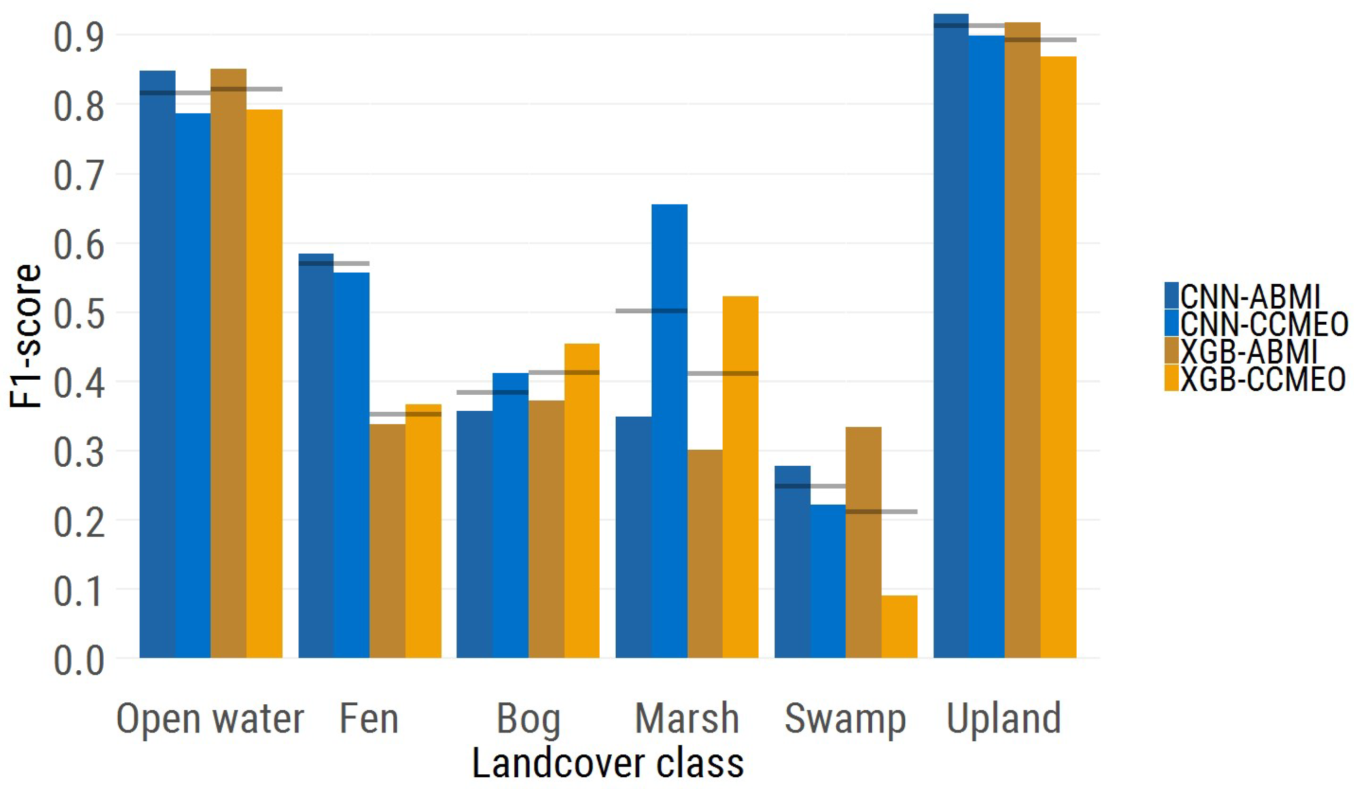
The per-class F1-scores for the ABMI and CCMEO data are seen in Figure 3 (blue showing the F1-score for the CNN model and orange the F1-score for the XGB model). The open water class shows almost equal F1-scores between the two models. The fen class F1-score is much higher in the CNN model (0.57) than the XGB model (0.35), while the bog score proved to be slightly higher in the XGB model. The marsh and swamp class both had a higher F1-score in the CNN model, although the F1-score were pretty poor for the swamp class (0.25 and 0.21 scores). Finally, the most numerous class, upland, showed a slightly higher F1-score in the CNN model.
When compared to the field validation data (AEP data), both products show a 50% overall accuracy on 22 points. In the CNN data, fen is correctly identified in six sites, but fen is also incorrectly predicted in five out of the seven bog sites (Table 4). In the XGB data, fen is predicted correctly in two of the six sites. XGB bog is more accurate than the CNN model, being correct in three of the seven sites. Open water appears to be similarly predicted in both products, with five out of nine sites being accurately predicted. Open water was incorrectly predicted as swamp or marsh in both models.
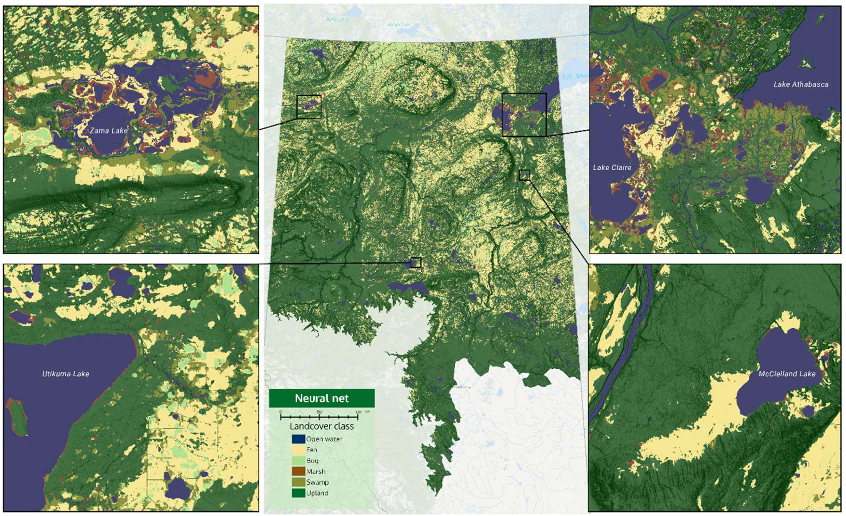
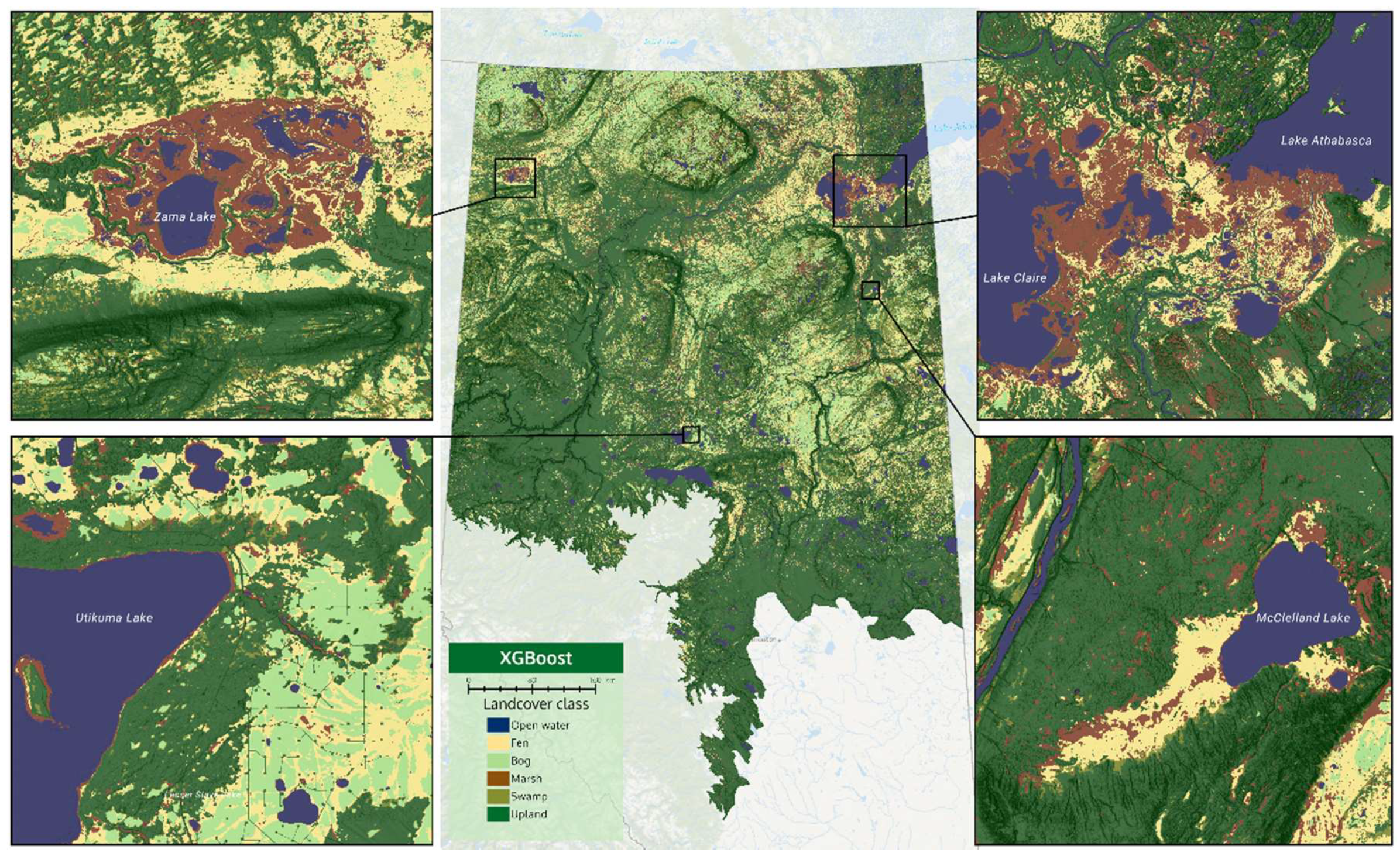
Visual results of the two products can be seen in Figure 4 and Figure 5. The four insets zoom into important wetland habitats in Alberta, which are described in the figure captions. An interactive side-by-side comparison of the two products can also be seen on a web map via this link (https://abmigc.users.earthengine.app/view/cnn-xgb). Additionally, the CNN product can be downloaded via this link (https://bit.ly/2X3Ao6N). We encourage readers to assess the visual aspects of these two products.
With reference to Figure 4 and Figure 5, and the web map, it is evident that CNN predictions produce smoother boundaries between wetland classes. The XGB model appears to produce speckled marsh at some locations (see McClelland fen—bottom-right inset of Figure 5). One of the major differences is the amount of bog versus fen predicted in the north-west portion of the province. The XGB model predicts massive areas of bog with small ribbons of fen, while the CNN model predicts about equal parts of fen and bog in these areas. Overall, the CNN model predicts: 4.8% open water, 19.0% fen, 3.0% bog, 1.0% marsh, 4.0% swamp, and 68.2% upland. The XGB model predicts: 4.4% open water, 10.8% fen, 9.3% bog, 5.0% marsh, 10.3% swamp, and 60.2% upland.

4. Discussion

This study produced two large-scale wetland inventory products using a fusion of open-access satellite data, and machine learning methods. The two machine learning approaches that were compared—convolutional neural networks and XGBoost—demonstrate a decent ability to predict wetland classes and upland habitat across a large region. Some wetland classes, such as bog and swamp, proved to be much harder to map. This is made clear in the relative F1-scores of the wetland classes (Figure 3). In the comparisons to the photo-interpretation validation data sets (Table 3), it is clear that the CNN model outperforms the XGB model in terms of overall accuracy, Kappa statistic, and per-class F1-score. As expected, the ABMI validation data proved to be slightly more accurate than the CCMEO validation data by 1–3%. This is still surprisingly close, given that the CCMEO data were completely independent from the model training process. The ABMI data were also an independent validation data set, but it is a subset of the data used to train the model. The CCMEO validation demonstrated a larger gap between the two models, with the CNN outperforming the XGB model by 8.2%. The ABMI data still showed a large, 5.7%, difference. The gap between the models is even more apparent when removing uplands, as the CNN model was 60.0% accurate, while the XGB model was 45.6% accurate. In terms of model development, both models took similar amounts of time to optimize, train, and predict (Table 2).
When comparing the products to field data, the results do not seem to be as promising. Both products had a 50% overall accuracy over 22 field sites. With reference to the field data, the CNN model clearly over-predicts fen, with 11 of the 13 wetland classes being predicted as fen, while the XGB model does not appear to have much ability to distinguish bog from fen (only 6 out of the 13 predicted correctly). We fully expect the overall accuracy of field data to go up if upland classes were included, but the main goal of this landcover classification was to map wetland classes. We believe less weight should be assigned to this accuracy assessment, given that is was just 22 points and it was just a small portion of the overall study area. Nevertheless, this does raise the question about how well landcover classifications actually match with what is seen on the ground. This may be something to test further when a larger field data set can be acquired. Right now, we cannot conclude if this is a real issue or a result of the small sample size. In the end, on the ground, wetland class is what actually matters for policy and planning, not what a photo-interpreter sees.
It appears that contextual information, texture, and convolutional filters help the CNN model better predict wetland class. The fen class is predicted much more accurately in the CNN model—0.57 versus 0.35 F1-score. This may be due to the parallel flow lines seen in many fen habitats (Figure 1), which can potentially be captured by certain convolutional filters. Marshes are also predicted more accurately in the CNN model. Here the CNN model likely uses contextual information about marshes, given marshes often surround water bodies. Visually, the CNN model appears to produce more ecologically meaningful wetland class boundaries. Boreal wetland classes are generally large, complex habitats, which can have multiple different vegetation types within one class. A large fen can be treed on the edges, then transition into shrub and graminoid fens at the center. Overall, it appears that the natural complexities of wetlands are better captured with a CNN model than a traditional pixel-based shallow learning (XGB) method. It is possible that an object-based wetland classification may also capture these natural complexities, but that is a question for future studies, as it was not in the scope of this project. We would also like to point out that the reference CNN was not subjected to rigorous optimization, and it is likely that there is still room for improvement in this model. This does tell us, though, that a naïve implementation of a CNN does outperform traditional shallow learning approaches for large-scale wetland mapping. Future work should focus on the ideal inputs for CNN wetland classification (i.e., spectral bands only, spectral bands + SAR, or handcrafted spectral features + SAR + topography).
Other studies have attempted similar deep learning wetland classifications in Canadian Boreal ecosystems. Pouliot et al. [51] tested a CNN wetland classification over a similar region in Alberta using Landsat data and reported 69% overall accuracy. Mahdianpari et al. [52] achieved a 96% wetland class accuracy in Newfoundland with RapidEye data and an InceptionResNetV2 algorithm. Mohammadimanesh et al. [20] reported a 93% wetland class accuracy again in Newfoundland using RADARSAT-2 data and a fully convolutional neural network. All of these demonstrated that deep learning results outperform other machine learning methods such as random forest. Non-neural network methods, such as the work in Amani et al. [83], reported a 71% wetland class accuracy across all of Canada. Another study by Mahdianpari et al. [34] achieved 88% wetland class accuracy using an object-based random forest algorithm across Newfoundland. In this study, the comparison between CNNs and shallow learning methods comes to the same conclusion as other recent studies; CNN/deep learning algorithms lead to better wetland classification results. The CNN product produced in this study does not achieve accuracies over 90% as seen in some smaller scale studies, likely because it is predicted across such a large area (397,958 km2). When compared to other large-scale wetland predictions, it appears to be one of the more accurate products, and thus it may prove useful for provincial/national wetland inventories. It also comes with the benefit of being produced with completely open-access data from Sentinel-1, Sentinel-2, and ALOS, and thus it can be easily updated to capture the dynamics of a changing Boreal landscape.
Large-scale wetland/landcover mapping in Canada seems to be converging towards a common methodology. Most studies are now using a fusion of remote sensing data from SAR, optical, and DEM products [6,7,34,39,49]. The easiest way to access provincial/national-scale data appears to be through Google Earth Engine; thus, many studies use Sentinel-1, Sentinel-2, Landsat, ALOS, or SRTM data [6,7,34,83]. Finally, many machine learning methods have been tested, but it appears that convolutional neural network frameworks produce better, more accurate wetland/landcover classifications [51,52]. This work contributes to these previous studies by confirming the value of CNNs. It also contributes to the greater goal of large-scale wetland mapping by demonstrating the ability to produce an accurate wetland inventory with a CNN and open-access satellite data.

5. Conclusions

The goal of this study was to compare shallow learning (XGB) and deep learning (CNN) methods for the production of a large-scale spatial wetland classification. We encourage readers to view both products via this link: https://abmigc.users.earthengine.app/view/cnn-xgb, and one of the products can be downloaded via this link: https://bit.ly/2X3Ao6N. A comparison of the two products to photo-interpreted validation data showed that CNN products outperform the shallow learning (XGB) product in terms of accuracy by about 5–8%. The CNN product achieved an average overall accuracy of 80.8% with a mean F1-score of 0.58. When compared to a small data set (n = 22) of field data, the results were inconclusive and both data sets showed little ability to distinguish between fen and bogs. This finding could just be due to the small, spatially constrained data or it could highlight the mismatch between on the ground conditions and large-scale landcover classifications.
Given the success of the CNN model in terms of accuracy, scalability, and production time, we believe this framework has the potential to provide credible landcover/wetland data for provinces, states, or countries. The use of Google Earth Engine and freely available imagery make the production of these inventories low cost with minimal processing time. The use of CNN deep learning algorithms produces products with ecologically meaningful boundaries and these algorithms are better able to capture the natural complexities of landcover classes such as wetlands. It appears that state-of-the-science large-scale inventories are moving towards deep learning-based classifications with freely available imagery accessed through Google Earth Engine. We hope other wetland/landcover mapping studies in Canada and abroad may benefit by using a similar approach to ours or by using our comparisons to inform model type choices.

Author Contributions

Conceptualization, E.R.D., J.F.S. and J.K.; development of CNN model and product, J.F.S.; development of XGB model and product, E.R.D.; analysis, E.R.D.; CCMEO validation data and accuracy assessment, M.M. and B.B.; AEP validation data and accuracy assessment, C.M.; writing—original draft preparation, E.R.D. and J.F.S.; writing—review and editing, M.M., B.B., C.M. and J.K.; funding acquisition, J.K.

Funding

This work was funded by the Alberta Biodiversity Monitoring Institute (ABMI). Funding in support of this work was received from the Alberta Environment and Parks.

Acknowledgments

Thanks to Liam Beaudette of the ABMI for the production of the SAGA topographic variables.

Conflicts of Interest

The authors declare no conflicts of interest.

Appendix A

Table A1. Confusion matrix comparing the CNN product to the ABMI plot validation data. UA is the user accuracy and PA is the producer accuracy.
Open waterFenBogMarshSwampUplandUA
Open water4483106328215420885.62
Fen3122,58039803787359320560.16
Bog049593129064949033.91
Marsh2935270142378162039.05
Swamp3843728622495927280741.58
Upland4937144339216613,525206,25889.71
PA83.9856.8937.6431.6420.8796.5781.32
Table A2. Confusion matrix comparing the XGB product to the ABMI plot validation data. UA is the user accuracy and PA is the producer accuracy.
Open waterFenBogMarshSwampUplandUA
Open water410333095491495.55
Fen498154211004272374453.47
Bog114,2146385273819153324.58
Marsh632434812524902312213520.68
Swamp4870681099270986212,28032.20
Upland550421028315168081193,88292.98
PA76.8624.7376.8155.3634.7390.7775.56
Table A3. Confusion matrix comparing the CNN product to the CCMEO validation data. UA is the user accuracy and PA is the producer accuracy.
Open waterFenBogMarshSwampUplandUA
Open water31841003184639182.32
Fen13013,9212828315100210,61848.31
Bog16262153212773459.10
Marsh262278230701746574.99
Swamp59138110252301959577118.79
Upland585489280614704128132,14891.75
PA75.4365.6731.5858.2427.0688.0280.28
Table A4. Confusion matrix comparing the XGB product to the CCMEO validation data. UA is the user accuracy and PA is the producer accuracy.
Open waterFenBogMarshSwampUplandUA
Open water28942406729993.78
Fen4973318351933663668039.10
Bog144280440838654316035.11
Marsh65418761593612172206742.30
Swamp4941761023197142817,3345.90
Upland561351139211641320120,78794.56
PA68.5634.5864.6668.5319.7380.4672.08

Appendix B

def get_unet(input_size, crop, num_channels, num_mask_channels, bn_axis=3):
    inputs = Input((input_size, input_size, num_channels))
    conv1 = Conv2D(32, (3, 3), padding=’same’, kernel_initializer=’he_uniform’)(inputs)
    conv1 = BatchNormalization(axis=bn_axis)(conv1)
    conv1 = keras.layers.advanced_activations.ELU()(conv1)
    conv1 = Conv2D(32, (3, 3), padding=’same’, kernel_initializer=’he_uniform’)(conv1)
    conv1 = BatchNormalization(axis=bn_axis)(conv1)
    conv1 = keras.layers.advanced_activations.ELU()(conv1)
    pool1 = MaxPooling2D(pool_size=(2, 2))(conv1)
    
    conv2 = Conv2D(64, (3, 3), padding=’same’, kernel_initializer=’he_uniform’)(pool1)
    conv2 = BatchNormalization(axis=bn_axis)(conv2)
    conv2 = keras.layers.advanced_activations.ELU()(conv2)
    conv2 = Conv2D(64, (3, 3), padding=’same’, kernel_initializer=’he_uniform’)(conv2)
    conv2 = BatchNormalization(axis=bn_axis)(conv2)
    conv2 = keras.layers.advanced_activations.ELU()(conv2)
    pool2 = MaxPooling2D(pool_size=(2, 2))(conv2)
    
    conv3 = Conv2D(128, (3, 3), padding=’same’, kernel_initializer=’he_uniform’)(pool2)
    conv3 = BatchNormalization(axis=bn_axis)(conv3)
    conv3 = keras.layers.advanced_activations.ELU()(conv3)
    conv3 = Conv2D(128, (3, 3), padding=’same’, kernel_initializer=’he_uniform’)(conv3)
    conv3 = BatchNormalization(axis=bn_axis)(conv3)
    conv3 = keras.layers.advanced_activations.ELU()(conv3)
    pool3 = MaxPooling2D(pool_size=(2, 2))(conv3)
    
    conv4 = Conv2D(256, (3, 3), padding=’same’, kernel_initializer=’he_uniform’)(pool3)
    conv4 = BatchNormalization(axis=bn_axis)(conv4)
    conv4 = keras.layers.advanced_activations.ELU()(conv4)
    conv4 = Conv2D(256, (3, 3), padding=’same’, kernel_initializer=’he_uniform’)(conv4)
    conv4 = BatchNormalization(axis=bn_axis)(conv4)
    conv4 = keras.layers.advanced_activations.ELU()(conv4)
    pool4 = MaxPooling2D(pool_size=(2, 2))(conv4)
    
    conv5 = Conv2D(512, (3, 3), padding=’same’, kernel_initializer=’he_uniform’)(pool4)
    conv5 = BatchNormalization(axis=bn_axis)(conv5)
    conv5 = keras.layers.advanced_activations.ELU()(conv5)
    conv5 = Conv2D(512, (3, 3), padding=’same’, kernel_initializer=’he_uniform’)(conv5)
    conv5 = BatchNormalization(axis=bn_axis)(conv5)
    conv5 = keras.layers.advanced_activations.ELU()(conv5)
    
    up6 = concatenate([UpSampling2D(size=(2, 2))(conv5), conv4], axis=3)
    conv6 = Conv2D(256, (3, 3), padding=’same’, kernel_initializer=’he_uniform’)(up6)
    conv6 = BatchNormalization(axis=bn_axis)(conv6)
    conv6 = keras.layers.advanced_activations.ELU()(conv6)
    conv6 = Conv2D(256, (3, 3), padding=’same’, kernel_initializer=’he_uniform’)(conv6)
    conv6 = BatchNormalization(axis=bn_axis)(conv6)
    conv6 = keras.layers.advanced_activations.ELU()(conv6)
    
    up7 = concatenate([UpSampling2D(size=(2, 2))(conv6), conv3], axis=3)
    conv7 = Conv2D(128, (3, 3), padding=’same’, kernel_initializer=’he_uniform’)(up7)
    conv7 = BatchNormalization(axis=bn_axis)(conv7)
    conv7 = keras.layers.advanced_activations.ELU()(conv7)
    conv7 = Conv2D(128, (3, 3), padding=’same’, kernel_initializer=’he_uniform’)(conv7)
    conv7 = BatchNormalization(axis=bn_axis)(conv7)
    conv7 = keras.layers.advanced_activations.ELU()(conv7)
    
    up8 = concatenate([UpSampling2D(size=(2, 2))(conv7), conv2], axis=3)
    conv8 = Conv2D(64, (3, 3), padding=’same’, kernel_initializer=’he_uniform’)(up8)
    conv8 = BatchNormalization(axis=bn_axis)(conv8)
    conv8 = keras.layers.advanced_activations.ELU()(conv8)
    conv8 = Conv2D(64, (3, 3), padding=’same’, kernel_initializer=’he_uniform’)(conv8)
    conv8 = BatchNormalization(axis=bn_axis)(conv8)
    conv8 = keras.layers.advanced_activations.ELU()(conv8)
    
    up9 = concatenate([UpSampling2D(size=(2, 2))(conv8), conv1], axis=3)
    conv9 = Conv2D(32, (3, 3), padding=’same’, kernel_initializer=’he_uniform’)(up9)
    conv9 = BatchNormalization(axis=bn_axis)(conv9)
    conv9 = keras.layers.advanced_activations.ELU()(conv9)
    conv9 = Conv2D(32, (3, 3), padding=’same’, kernel_initializer=’he_uniform’)(conv9)
    crop9 = Cropping2D(cropping=((crop, crop), (crop, crop)))(conv9)
    conv9 = BatchNormalization(axis=bn_axis)(crop9)
    conv9 = keras.layers.advanced_activations.ELU()(conv9)
    conv10 = Conv2D(num_mask_channels, (1, 1), activation=’sigmoid’)(conv9)
    
    model = Model(inputs=inputs, outputs=conv10)
    return model
    
Code 1: Sample U-Net function used to produce the CNN model predictions.

References

  1. Chollet, F.; Allaire, J. Deep Learning with R; Manning Publications Co.: Greenwich, CT, USA, 2018. [Google Scholar]
  2. Guo, Y.; Liu, Y.; Oerlemans, A.; Lao, S.; Wu, S.; Lew, M.S. Deep learning for visual understanding: A review. Neurocomputing 2016, 187, 27–48. [Google Scholar] [CrossRef]
  3. Voulodimos, A.; Doulamis, N.; Doulamis, A.; Protopapadakis, E. Deep learning for computer vision: A brief review. Comput. Intell. Neurosci. 2018, 2018, 7068349. [Google Scholar] [CrossRef] [PubMed]
  4. Pal, M. Random forest classifier for remote sensing classification. Int. J. Remote Sens. 2005, 26, 217–222. [Google Scholar] [CrossRef]
  5. Pal, M.; Mather, P. Support vector machines for classification in remote sensing. Int. J. Remote Sens. 2005, 26, 1007–1011. [Google Scholar] [CrossRef]
  6. Hird, J.; DeLancey, E.; McDermid, G.; Kariyeva, J. Google Earth Engine, open-access satellite data, and machine learning in support of large-area probabilistic wetland mapping. Remote Sens. 2017, 9, 1315. [Google Scholar] [CrossRef] [Green Version]
  7. DeLancey, E.R.; Kariyeva, J.; Bried, J.; Hird, J. Large-scale probabilistic identification of boreal peatlands using Google Earth Engine, open-access satellite data, and machine learning. PLoS ONE 2019, 14, e0218165. [Google Scholar] [CrossRef] [PubMed] [Green Version]
  8. Cortes, C.; Vapnik, V. Support-vector networks. Mach. Learn. 1995, 20, 273–297. [Google Scholar] [CrossRef]
  9. Quinlan, J.R. Induction of decision trees. Mach. Learn. 1986, 1, 81–106. [Google Scholar] [CrossRef] [Green Version]
  10. Chen, T.; Guestrin, C. Xgboost: A scalable tree boosting system. In Proceedings of the 22nd acm sigkdd international conference on knowledge discovery and data mining, San Francisco, CA, USA, 13–17 August 2016; pp. 785–794. [Google Scholar]
  11. Gurney, C.M.; Townshend, J.R. The use of contextual information in the classification of remotely sensed data. Photogramm. Eng. Remote Sens. 1983, 49, 55–64. [Google Scholar]
  12. Blaschke, T. Object based image analysis for remote sensing. ISPRS J. Photogramm. Remote Sens. 2010, 65, 2–16. [Google Scholar] [CrossRef] [Green Version]
  13. Stumpf, A.; Kerle, N. Object-oriented mapping of landslides using random forests. Remote Sens. Environ. 2011, 115, 2564–2577. [Google Scholar] [CrossRef]
  14. Ma, L.; Liu, Y.; Zhang, X.; Ye, Y.; Yin, G.; Johnson, B.A. Deep learning in remote sensing applications: A meta-analysis and review. ISPRS J. Photogramm. Remote Sens. 2019, 152, 166–177. [Google Scholar] [CrossRef]
  15. Zhang, L.; Zhang, L.; Du, B. Deep learning for remote sensing data: A technical tutorial on the state of the art. IEEE Geosci. Remote Sens. Mag. 2016, 4, 22–40. [Google Scholar] [CrossRef]
  16. Makantasis, K.; Karantzalos, K.; Doulamis, A.; Doulamis, N. Deep supervised learning for hyperspectral data classification through convolutional neural networks. In Proceedings of the 2015 IEEE International Geoscience and Remote Sensing Symposium (IGARSS), Milan, Italy, 26–31 July 2015; pp. 4959–4962. [Google Scholar]
  17. Zhu, X.X.; Tuia, D.; Mou, L.; Xia, G.-S.; Zhang, L.; Xu, F.; Fraundorfer, F. Deep learning in remote sensing: A comprehensive review and list of resources. IEEE Geosci. Remote Sens. Mag. 2017, 5, 8–36. [Google Scholar] [CrossRef] [Green Version]
  18. Makantasis, K.; Karantzalos, K.; Doulamis, A.; Loupos, K. Deep learning-based man-made object detection from hyperspectral data. In Proceedings of the International Symposium on Visual Computing, Las Vegas, NV, USA, 14–16 December 2015; pp. 717–727. [Google Scholar]
  19. Rezaee, M.; Mahdianpari, M.; Zhang, Y.; Salehi, B. Deep convolutional neural network for complex wetland classification using optical remote sensing imagery. IEEE J. Sel. Top. Appl. Earth Obs. Remote Sens. 2018, 11, 3030–3039. [Google Scholar] [CrossRef]
  20. Mohammadimanesh, F.; Salehi, B.; Mahdianpari, M.; Gill, E.; Molinier, M. A new fully convolutional neural network for semantic segmentation of polarimetric SAR imagery in complex land cover ecosystem. ISPRS J. Photogramm. Remote Sens. 2019, 151, 223–236. [Google Scholar] [CrossRef]
  21. Ball, J.E.; Anderson, D.T.; Chan, C.S. Comprehensive survey of deep learning in remote sensing: Theories, tools, and challenges for the community. J. Appl. Remote Sens. 2017, 11, 042609. [Google Scholar] [CrossRef] [Green Version]
  22. Ronneberger, O.; Fischer, P.; Brox, T. U-net: Convolutional networks for biomedical image segmentation. In Proceedings of the International Conference on Medical image computing and computer-assisted intervention, Munich, Germany, 5–9 October 2015; pp. 234–241. [Google Scholar]
  23. Zoltai, S.; Vitt, D. Canadian wetlands: Environmental gradients and classification. Vegetatio 1995, 118, 131–137. [Google Scholar] [CrossRef]
  24. Nahlik, A.; Fennessy, M. Carbon storage in US wetlands. Nat. Commun. 2016, 7, 13835. [Google Scholar] [CrossRef] [Green Version]
  25. Assessment, M.E. Ecosystems and Human Well-Being: Wetlands and Water; World Resources Institute: Washington, DC, USA, 2005. [Google Scholar]
  26. Brinson, M.M.; Malvárez, A.I. Temperate freshwater wetlands: Types, status, and threats. Environ. Conserv. 2002, 29, 115–133. [Google Scholar] [CrossRef]
  27. Mitsch, W.J.; Bernal, B.; Nahlik, A.M.; Mander, Ü.; Zhang, L.; Anderson, C.J.; Jørgensen, S.E.; Brix, H. Wetlands, carbon, and climate change. Landsc. Ecol. 2013, 28, 583–597. [Google Scholar] [CrossRef]
  28. Erwin, K.L. Wetlands and global climate change: The role of wetland restoration in a changing world. Wetl. Ecol. Manag. 2009, 17, 71. [Google Scholar] [CrossRef]
  29. Waddington, J.; Morris, P.; Kettridge, N.; Granath, G.; Thompson, D.; Moore, P. Hydrological feedbacks in northern peatlands. Ecohydrology 2015, 8, 113–127. [Google Scholar] [CrossRef]
  30. Alberta Environment and Parks. Alberta Merged Wetland Inventory; Alberta Environment and Parks: Edmonton, AB, Canada, 2017. [Google Scholar]
  31. Willier, C. Changes in peatland plant community composition and stand structure due to road induced flooding and desiccation. University of Alberta: Edmonton, AB, Canada, 2017. [Google Scholar]
  32. Heijmans, M.M.; Mauquoy, D.; Van Geel, B.; Berendse, F. Long-term effects of climate change on vegetation and carbon dynamics in peat bogs. J. Veg. Sci. 2008, 19, 307–320. [Google Scholar] [CrossRef] [Green Version]
  33. Johnson, W.C.; Millett, B.V.; Gilmanov, T.; Voldseth, R.A.; Guntenspergen, G.R.; Naugle, D.E. Vulnerability of northern prairie wetlands to climate change. BioScience 2005, 55, 863–872. [Google Scholar] [CrossRef]
  34. Mahdianpari, M.; Salehi, B.; Mohammadimanesh, F.; Homayouni, S.; Gill, E. the first wetland inventory map of newfoundland at a spatial resolution of 10 m using sentinel-1 and sentinel-2 data on the google earth engine cloud computing platform. Remote Sens. 2019, 11, 43. [Google Scholar] [CrossRef] [Green Version]
  35. Mahdavi, S.; Salehi, B.; Granger, J.; Amani, M.; Brisco, B.; Huang, W. Remote sensing for wetland classification: A comprehensive review. Gisci. Remote Sens. 2018, 55, 623–658. [Google Scholar] [CrossRef]
  36. Tiner, R.W. Wetland Indicators: A Guide to Wetland Identification, Delineation, Classification, and Mapping; CRC Press: Baco Raton, FL, USA, 1999. [Google Scholar]
  37. Bourgeau-Chavez, L.; Kasischke, E.; Brunzell, S.; Mudd, J.; Smith, K.; Frick, A. Analysis of space-borne SAR data for wetland mapping in Virginia riparian ecosystems. Int. J. Remote Sens. 2001, 22, 3665–3687. [Google Scholar] [CrossRef]
  38. Brisco, B. Mapping and monitoring surface water and wetlands with synthetic aperture radar. In Remote Sensing of Wetlands: Applications and Advances; Tiner, R.W., Lang, M.W., Klemas, V.V., Eds.; CRC Press: Boca Raton, FL, USA, 2015; pp. 119–136. [Google Scholar]
  39. Amani, M.; Salehi, B.; Mahdavi, S.; Granger, J.; Brisco, B. Wetland classification in Newfoundland and Labrador using multi-source SAR and optical data integration. Gisci. Remote Sens. 2017, 54, 779–796. [Google Scholar] [CrossRef]
  40. DeLancey, E.R.; Kariyeva, J.; Cranston, J.; Brisco, B. Monitoring hydro temporal variability in Alberta, Canada with multi-temporal Sentinel-1 SAR data. Can. J. Remote Sens. 2018, 44, 1–10. [Google Scholar] [CrossRef]
  41. Montgomery, J.; Hopkinson, C.; Brisco, B.; Patterson, S.; Rood, S.B. Wetland hydroperiod classification in the western prairies using multitemporal synthetic aperture radar. Hydrol. Process. 2018, 32, 1476–1490. [Google Scholar] [CrossRef]
  42. Montgomery, J.; Brisco, B.; Chasmer, L.; Devito, K.; Cobbaert, D.; Hopkinson, C. SAR and Lidar Temporal Data Fusion Approaches to Boreal Wetland Ecosystem Monitoring. Remote Sens. 2019, 11, 161. [Google Scholar] [CrossRef] [Green Version]
  43. Touzi, R.; Deschamps, A.; Rother, G. Wetland characterization using polarimetric RADARSAT-2 capability. Can. J. Remote Sens. 2007, 33, S56–S67. [Google Scholar] [CrossRef]
  44. White, L.; Brisco, B.; Dabboor, M.; Schmitt, A.; Pratt, A. A collection of SAR methodologies for monitoring wetlands. Remote Sens. 2015, 7, 7615–7645. [Google Scholar] [CrossRef] [Green Version]
  45. White, L.; Brisco, B.; Pregitzer, M.; Tedford, B.; Boychuk, L. RADARSAT-2 beam mode selection for surface water and flooded vegetation mapping. Can. J. Remote Sens. 2014, 40, 135–151. [Google Scholar]
  46. Amani, M.; Salehi, B.; Mahdavi, S.; Granger, J.; Brisco, B. Evaluation of multi-temporal landsat 8 data for wetland classification in newfoundland, Canada. In Proceedings of the 2017 IEEE International Geoscience and Remote Sensing Symposium (IGARSS), Fort Worth, TX, USA, 23–28 July 2017; pp. 6229–6231. [Google Scholar]
  47. Wulder, M.; Li, Z.; Campbell, E.; White, J.; Hobart, G.; Hermosilla, T.; Coops, N. A national assessment of wetland status and trends for Canada’s forested ecosystems using 33 years of Earth observation satellite data. Remote Sens. 2018, 10, 1623. [Google Scholar] [CrossRef] [Green Version]
  48. Grenier, M.; Demers, A.-M.; Labrecque, S.; Benoit, M.; Fournier, R.A.; Drolet, B. An object-based method to map wetland using RADARSAT-1 and Landsat ETM images: Test case on two sites in Quebec, Canada. Can. J. Remote Sens. 2007, 33, S28–S45. [Google Scholar] [CrossRef]
  49. Merchant, M.A.; Warren, R.K.; Edwards, R.; Kenyon, J.K. An object-based assessment of multi-wavelength sar, optical imagery and topographical datasets for operational wetland mapping in Boreal Yukon, Canada. Can. J. Remote Sens. 2019, 45, 308–332. [Google Scholar] [CrossRef]
  50. Dronova, I. Object-based image analysis in wetland research: A review. Remote Sens. 2015, 7, 6380–6413. [Google Scholar] [CrossRef] [Green Version]
  51. Pouliot, D.; Latifovic, R.; Pasher, J.; Duffe, J. Assessment of Convolution Neural Networks for Wetland Mapping with Landsat in the Central Canadian Boreal Forest Region. Remote Sens. 2019, 11, 772. [Google Scholar] [CrossRef] [Green Version]
  52. Mahdianpari, M.; Salehi, B.; Rezaee, M.; Mohammadimanesh, F.; Zhang, Y. Very deep convolutional neural networks for complex land cover mapping using multispectral remote sensing imagery. Remote Sens. 2018, 10, 1119. [Google Scholar] [CrossRef] [Green Version]
  53. Natural Regions Committee. Natural regions and subregions of Alberta; Downing, D.J., Pettapiece, W.W., Eds.; Government of Alberta: Edmonton, AB, Canada, 2006.
  54. ABMI. Human Footprint Inventory 2016; ABMI: Edmonton, AB, Canada, 2018. [Google Scholar]
  55. Alberta Environment and Sustainable Resource Development. Alberta Wetland Classification System; Water Policy Branch, Policy and Planning Division: Edmonton, AB, Canada, 2015. [Google Scholar]
  56. Gorham, E. Northern peatlands: Role in the carbon cycle and probable responses to climatic warming. Ecol. Appl. 1991, 1, 182–195. [Google Scholar] [CrossRef] [PubMed]
  57. Vitt, D.H. An overview of factors that influence the development of Canadian peatlands. Mem. Entomol. Soc. Can. 1994, 126, 7–20. [Google Scholar] [CrossRef]
  58. Vitt, D.H.; Chee, W.-L. The relationships of vegetation to surface water chemistry and peat chemistry in fens of Alberta, Canada. Vegetatio 1990, 89, 87–106. [Google Scholar] [CrossRef]
  59. Warner, B.; Rubec, C. The Canadian Wetland Classification System; Wetlands Research Centre, University of Waterloo: Waterloo, ON, Canada, 1997. [Google Scholar]
  60. Gorelick, N.; Hancher, M.; Dixon, M.; Ilyushchenko, S.; Thau, D.; Moore, R. Google Earth Engine: Planetary-scale geospatial analysis for everyone. Remote Sens. Environ. 2017, 202, 18–27. [Google Scholar] [CrossRef]
  61. Gauthier, Y.; Bernier, M.; Fortin, J.-P. Aspect and incidence angle sensitivity in ERS-1 SAR data. Int. J. Remote Sens. 1998, 19, 2001–2006. [Google Scholar] [CrossRef]
  62. Bruniquel, J.; Lopes, A. Multi-variate optimal speckle reduction in SAR imagery. Int. J. Remote Sens. 1997, 18, 603–627. [Google Scholar] [CrossRef]
  63. Housman, I.; Hancher, M.; Stam, C. A quantitative evaluation of cloud and cloud shadow masking algorithms available in Google Earth Engine. manuscript in preparation.
  64. Conrad, O.; Bechtel, B.; Bock, M.; Dietrich, H.; Fischer, E.; Gerlitz, L.; Wehberg, J.; Wichmann, V.; Böhner, J. System for automated geoscientific analyses (SAGA) v. 2.1. 4. Geosci. Model Dev. 2015, 8, 1991–2007. [Google Scholar] [CrossRef] [Green Version]
  65. ABMI. ABMI 3x7 Photoplot Land Cover Dataset Data Model; ABMI: Edmonton, AB, Canada, 2016. [Google Scholar]
  66. Drusch, M.; Del Bello, U.; Carlier, S.; Colin, O.; Fernandez, V.; Gascon, F.; Hoersch, B.; Isola, C.; Laberinti, P.; Martimort, P. Sentinel-2: ESA’s optical high-resolution mission for GMES operational services. Remote Sens. Environ. 2012, 120, 25–36. [Google Scholar] [CrossRef]
  67. Gitelson, A.A.; Merzlyak, M.N.; Chivkunova, O.B. Optical properties and nondestructive estimation of anthocyanin content in plant leaves. Photochem. Photobiol. 2001, 74, 38–45. [Google Scholar] [CrossRef]
  68. Rouse, J.W., Jr.; Haas, R.; Schell, J.; Deering, D. Monitoring vegetation systems in the Great Plains with ERTS. 1974. Available online: https://ntrs.nasa.gov/archive/nasa/casi.ntrs.nasa.gov/19740022614.pdf (accessed on 23 November 2019).
  69. McFeeters, S.K. The use of the Normalized Difference Water Index (NDWI) in the delineation of open water features. Int. J. Remote Sens. 1996, 17, 1425–1432. [Google Scholar] [CrossRef]
  70. Hatfield, J.L.; Prueger, J.H. Value of using different vegetative indices to quantify agricultural crop characteristics at different growth stages under varying management practices. Remote Sens. 2010, 2, 562–578. [Google Scholar] [CrossRef] [Green Version]
  71. Herrmann, I.; Pimstein, A.; Karnieli, A.; Cohen, Y.; Alchanatis, V.; Bonfil, D. Assessment of leaf area index by the red-edge inflection point derived from VENμS bands. In Proceedings of the ESA hyperspectral workshop, Frascati, Italy, 17–19 March 2010; pp. 1–7. [Google Scholar]
  72. Weiss, A. Topographic position and landforms analysis. In Proceedings of the Poster Presentation, ESRI User Conference, San Diego, CA, USA, 9–13 July 2001; Volume 200. [Google Scholar]
  73. Böhner, J.; Kothe, R.; Conrad, O.; Gross, J.; Ringeler, A.; Selige, T. Soil regionalisation by means of terrain analysis and process parameterisation. European soil Bureau Research Report NO. 7 2002. Available online: https://www.researchgate.net/publication/284700427_Soil_regionalisation_by_means_of_terrain_analysis_and_process_parameterisation (accessed on 11 November 2019).
  74. Gallant, J.C.; Dowling, T.I. A multiresolution index of valley bottom flatness for mapping depositional areas. Water Resour. Res. 2003, 39. [Google Scholar] [CrossRef]
  75. Chen, T.; He, T. Xgboost: Extreme Gradient Boosting, R Package Version 0.4-2; Available online: https://cran.r-project.org/web/packages/xgboost/vignettes/xgboost.pdf (accessed on 1 August 2019).
  76. R Core Team. R: A language and Environment for Statistical Computing; R Foundation for Statistical Computing; Vienna, Austria, 2013. [Google Scholar]
  77. Hacker Earth. Beginners Tutorial on XGBoost and Parameter Tuning in R. Available online: https://www.hackerearth.com/practice/machine-learning/machine-learning-algorithms/beginners-tutorial-on-xgboost-parameter-tuning-r/tutorial/ (accessed on 29 August 2019).
  78. Parisien, M.-A.; Parks, S.A.; Miller, C.; Krawchuk, M.A.; Heathcott, M.; Moritz, M.A. Contributions of ignitions, fuels, and weather to the spatial patterns of burn probability of a boreal landscape. Ecosystems 2011, 14, 1141–1155. [Google Scholar] [CrossRef]
  79. Atienza, R. Advanced Deep Learning with Keras: Apply Deep Learning Techniques, Autoencoders, Gans, Variational Autoencoders, Deep Reinforcement Learning, Policy Gradients, and More; Packt Publishing Ltd.: Birmingham, UK, 2018. [Google Scholar]
  80. Basu, S.; Ganguly, S.; Mukhopadhyay, S.; DiBiano, R.; Karki, M.; Nemani, R. Deepsat: A learning framework for satellite imagery. In Proceedings of the 23rd SIGSPATIAL international conference on advances in geographic information systems, Seattle, WA, USA, 3–6 November 2015; p. 37. [Google Scholar]
  81. Kaggle. Dstl Satellite Imagery Competition, 3rd Place Winners’ Interview: Vladimir & Sergey. Available online: http://blog.kaggle.com/2017/05/09/dstl-satellite-imagery-competition-3rd-place-winners-interview-vladimir-sergey/ (accessed on 29 November 2019).
  82. Dozat, T. Incorporating Nesterov Momentum into Adam. 2016. Available online: https://openreview.net/pdf?id=OM0jvwB8jIp57ZJjtNEZ (accessed on 12 December 2019).
  83. Amani, M.; Mahdavi, S.; Afshar, M.; Brisco, B.; Huang, W.; Mohammad Javad Mirzadeh, S.; White, L.; Banks, S.; Montgomery, J.; Hopkinson, C. Canadian wetland inventory using google earth engine: The first map and preliminary results. Remote Sens. 2019, 11, 842. [Google Scholar] [CrossRef] [Green Version]
Figure 1. Top panel: Distribution of pixel values for four common remote sensing and topographic indicators of wetlands: Topographic Wetness Index (TWI), Vertical Vertical backscatter of Sentinel-1 (VV), Normalized Difference Vegetation Index (NDVI), and delta Normalized Difference Vegetation Index fall–spring (dNDVI). These violin plots are generated from random points placed in 50,000 polygons for each wetland class. Bottom panel: Visualization of the four wetland classes in the Alberta Biodiversity Monitoring Institute (ABMI) plot data (colors the same as the top panel) with ESRI base layer imagery. Upland areas are masked out of the ABMI plot visualization.
Remotesensing 12 00002 g001
Figure 2. Location of the study area (red), ABMI plots used for validation (orange), ABMI plots used for training and pre-prediction validation (black), location of the Canadian Centre for Mapping and Earth Observation (CCMEO) validation data (purple), and Alberta Environment and Parks (AEP) field data location (blue) overlain on an elevation background.
Remotesensing 12 00002 g002
Figure 3. Summary of per-class F1-scores for all validation exercises. The CNN F1-scores are in shades of blue and the XGB f-scores are in shades of orange. The averages across the two validation exercises are the semi-transparent black lines.
Remotesensing 12 00002 g003
Figure 4. Convolutional neural network prediction of landcover class across the Boreal region. The insets zoom in on important wetland landscapes in the Boreal region. Top-left: Zama Lake wetland area; bottom-right: Utikuma Lake; top-right: The Peace Athabasca Delta; and bottom-right: The McClelland Lake fen/wetland complex.
Remotesensing 12 00002 g004
Figure 5. XGBoost prediction of landcover class across the Boreal region. The insets zoom in on important wetland landscapes in the Boreal region. Top-left: Zama Lake wetland area; bottom-right: Utikuma Lake; top-right: The Peace Athabasca Delta; and bottom-right: the McClelland Lake fen/wetland complex.
Remotesensing 12 00002 g005
Table 1. List of input variables in the XGBoost model (XGB) and convolutional neural network (CNN) models. Each variable lists its respective data source, equation, description, and, if needed, citation. For information on Sentinel-2 band information not listed in the table, see: [66] and https://sentinel.esa.int/web/sentinel/user-guides/sentinel-2-msi/resolutions/spatial.
VariableData sourceModelEquationDescription
ARISentinel-2XGB/CNN ( B 8 B 2 )     ( B 8 B 3 )   Anthocyanin Reflectance Index. An index sensitive to anthocyanin pigments in plant foliage, which is often associated with plant stress or senescence [67].
Band 2Sentinel-2CNN-The blue band of Sentinel-2. Central wavelength at 492 nm.
Band 3Sentinel-2CNN-The green band of Sentinel-2. Central wavelength at 559 nm.
Band 4Sentinel-2CNN-The blue band of Sentinel-2. Central wavelength at 664 nm.
DEMALOSCNN-The raw elevation values from the ALOS DEM.
NDVISentinel-2CNN ( B 8   B 4 ) ( B 8   +   B 4 ) Normalized Difference Vegetation Index. Index for estimating photosynthetic activity and leaf area [68].
dNDVISentinel-2XGB N D V I f a l l   N D V I s u m m e r The change in NDVI from fall to summer.
NDWISentinel-2CNN ( B 3   B 8 ) ( B 3   +   B 8 ) Normalized Difference Water Index from [69].
POLrSentinel-1XGB V H V V The ratio between the VH and VV polarization.
PSRISentinel-2CNN ( B 4   B 2 ) ( B a n d   5 ) Plant Senescence Reflectance Index. A ratio used to estimate the ratio of bulk carotenoids to chlorophyll [70].
REIPSentinel-2XGB/CNN 702 + 40 ( ( B 4 + B 7 2 ) B 5 ( B 6 B 5 ) ) Red Edge Inflection Point. An approximation on a hyperspectral index for estimating the position (in nm) of the NIR/red inflection point in vegetation spectra [71].
TPIALOSXGB/CNN-Topographic Position Index (TPI) generated in SAGA [64]. An index describing the relative position of a pixel within a valley, ridge top continuum calculated in a given window size. TPI was calculated with a 750 m moving window for this purpose [72]. Justification for this size can be seen in [7].
TRIALOSCNN Topographic Roughness Index generated in SAGA.
TWIALOSXGB/CNN-Saga Wetness Index. A SAGA version of the Topographic Wetness Index. Potential wetness of the ground based on topography [73].
VBFALOSXGB/CNN-Multi Resolution Index of Valley Bottom Flatness [74]. This index measures the degree of valley bottom flatness at multiple scales. Large flat valleys are typical landscapes for wetland formation.
VH Sentinel-1XGB/CNN-Vertical polarization sending horizontal polarization receiving SAR backscatter in decibels.
dVHSentinel-1XGB V H w i n t e r   V H s u m m e r The change in VH backscatter from winter to summer.
Table 2. Full comparison of training time, prediction time, optimization time (i.e., time to properly tune the model), and hardware for each model.
ModelTraining Time (Hours)Prediction Time (Hours)Optimization Time (Hours)Hardware
CNN44UnknownDesktop with 64 Gb of RAM and one Titan X (Maxwell) GPU.
XGB472—can be reduced by distributing prediction to more cores or more machines.2Desktop with 64 GB of ram and 64 logical cores.
Table 3. Model validation statistics (overall accuracy, Kappa statistic, and mean F1-score) of the CNN and XGB models for the two independent validation data sets.
Validation DataModelOverall Accuracy (%)Kappa StatisticMean F1-Score
ABMI plotsCNN81.30.570.56
ABMI plotsXGB75.60.490.52
CCMEOCNN80.30.520.59
CCMEOXGB72.10.410.52
Table 4. Confusion matrix for the CNN and XGB accuracy assessment against the AEP field validation data. Columns represent reference wetland class, while the rows represent the predicted wetland class.
PredictionReference—CNNPredictionReference—XGB
Open waterFenBogOpen waterFenBog
Open water500Open water500
Fen065Fen023
Bog000Bog004
Marsh100Marsh240
Swamp001Swamp000
Upland301Upland200

