Abstract
The use of infrared (IR) sensors to detect clouds in different layers of the atmosphere is a big challenge, especially for ice clouds. This study aims to improve ice cloud detection using Lin’s algorithm and apply it to Atmospheric Infrared Sounder (AIRS). To achieve these objectives, the scattering and emission characteristics of clouds as perceived by AIRS longwave infrared (LWIR, ~15 μm) and shortwave infrared (SWIR, ~4.3 μm) CO2 absorption bands are applied for ice cloud detection. Hence, the weighting function peak (WFP), cut-off pressure, and correlation coefficients between the brightness temperatures (BTs) of LWIR and SWIR channels are used to pair the LWIR and SWIR channels. After that, the linear relationship between the clear-sky BTs of the paired LWIR and SWIR channels is established by the cloud scattering and emission Index (CESI). However, the linear relationship fails in the presence of ice clouds. Comparing these results with collocated Cloud-Aerosol Lidar with Orthogonal Polarization (CALIOP) observations show that the probability of detection of ice clouds for Pair-8 (WFP~330hPa), Pair-19 (WFP~555hPa), and Pair-24 (WFP~866hPa) are 0.63, 0.71, and 0.73 in the daytime and 0.46, 0.62, and 0.7 in the nighttime at a false alarm rate of 0.1 when ice clouds top pressure above 330 hPa, 555 hPa, and 866 hPa, respectively. Furthermore, the thresholds of the three pairs are 2.4 K, 3 K, and 8.7 K in the daytime and 1.7 K, 1.7 K, and 4.4 K in the nighttime at the highest Heike Skill Score (HSS). The error of HSS values based on thresholds of ice clouds is between 0.01 and 0.02 which is comparable with the ice cloud detection results in both day and night conditions. It is shown that Pair-8 (WFP~330hPa) can detect opaque and thick ice clouds above its WFP altitude over the tropical areas but it is unable to observe ice clouds over the mid-latitude while Pair-19 and Pair-24 can identify ice clouds above their WFP altitude.
1. Introduction
Ice clouds, consisting of various types of ice crystals, absorb thermal infrared emission from the lower atmosphere and surface and reflect solar radiation, thus regulating the Earth’s radiation budget [1,2,3]. Cloud detection, especially for ice clouds, plays a significant role in most algorithms by using satellite radiance data [4]. It not only affects the retrieving atmospheric or surface information but gives rises to the data assimilation for numerical weather prediction [5,6].
The Atmospheric Infrared Sounder (AIRS), a hyperspectral infrared sensor, is designed to support weather forecast and climate research [7,8,9]. Its improved spectral resolution leads to enhancement of the vertical resolution, thermal resolution, and accuracy with respect to the concentration of absorbing gases (such as ozone and water vapor) than the previous High-Resolution Infrared Radiation Sounder (HIRS) [10]. Indeed, AIRS data have been widely used to improve numerical weather predictions (NWPs), retrieving atmospheric profiles, trace gases, and cloud characteristics [8,11,12,13,14,15,16].
The method to determine the brightness temperature difference (BTD) threshold has been widely used to detect ice clouds and has been applied to infrared imagers, such as Infrared Interferometer Spectrometer (IRIS) [17], Advanced Very High Resolution Radiometer (AVHRR) [18,19], Moderate Resolution Imaging Spectroradiometer (MODIS) [20], and the Visible Infrared Imager Radiometer Suite (VIIRS) [21,22]. For hyperspectral infrared sounders, McNally and Watts [23] developed a cloud detection method that ranks the channels according to the sensitivity of channels to clouds and uses the channels whose weighting function peak altitude above the cloud top level to assimilate numerical weather prediction and discard lower ones. However, there are some biases from instrument noise, forward model, and background of the atmosphere [24]. Additionally, the Multivariate and Minimum Residual (MMR) methods, developed in 2014, simulate the cloudy radiances variation to fit the observation to identify the channel affected by clouds [25,26]. Furthermore, Amato et al. [27] used the cumulative discriminant analysis to detect clouds by minimizing a cost function. Even though these methods for a hyperspectral sounder have the ability to detect clouds or discriminate between cloudy and clear fields of view (FOVs), most of these methods do not focus on the cloud phase classification and cloud top pressure. For the ice cloud detection, the window channels have been used to detect ice clouds for hyperspectral sounders [28,29].
However, it is still a challenge to detect ice clouds in certain vertical atmospheric layers because of the selection of the channels. CO2 absorption channels in the infrared region provide the opportunity to detect clouds in different layers of atmosphere. This is because CO2 is mixed almost uniformly in the air and can provide information about atmospheric temperature profiles over the globe [30]. The longwave 15 μm CO2 absorption band has been used to obtain cloud altitudes, effective cloud amounts, and atmospheric temperature profiles in the CO2 slicing method [31,32,33]. The shortwave 4.3 μm CO2 absorption band is employed to derive the upper atmospheric temperature as well [34]. Furthermore, Gao et al. [35] combined shortwave CO2 absorption bands with N2O that had similar properties as the 15 μm CO2 channels.
In 2017, Lin et al. [24] (hereafter Lin17) introduced a new algorithm to detect clouds in different atmospheric layers. The method uses the Cross-track Infrared Sounder (CrIS) longwave (~15 μm) and shortwave (~4.3 μm) infrared CO2 absorption bands, and it is based on the fact that the scattering and emission properties of longwave and shortwave CO2 channels at the similar height (or pressure level) are different and distinguishable. This method has a significant advantage that the algorithm is simple and can use observed brightness temperature of corresponding CO2 infrared channels to detect clouds in certain vertical atmospheric layers. Wang et al. [36] (hereafter Wang19) used VIIRS to assess cloud emission and scattering index (CESI) from Lin17 and used Linear Discriminant Analysis (LDA) to combine low peak weighting function pairs to improve the detection of cirrus. However, there are some shortcomings from Lin17 and Wang19. In Lin17, the cloud scheme was based on simulated BT from European Centre for Medium-Range Weather Forecasts (ECMWF) profiles and the radiative transfer model. Even though the derived cloud scheme has the ability to detect clouds, the scheme lack of real observation from sensors and the impact of solar radiation for SWIR in the daytime was not considered. Further, the exact threshold values of cloud scheme were not obtained from Lin17 in different atmospheric layers. In Wang19, the passive imager VIIRS was employed to compensate for the cirrus detection thresholds but there are some flaws from VIIRS retrieved algorithm. In VIIRS cloud mask algorithm, the strong water vapor absorption band of the 1.38 μm channel was employed to detect thin cirrus in the daytime. However, the 1.38 μm channel was not appropriate to detect cirrus in elevated surfaces and dry atmospheric conditions [37]. Further, the cloud top pressure of cirrus was not considered in Wang19.
This study fully developed a retrieval algorithm based on dual CO2 absorption bands and Lin’s methods, and tested the method using actual satellite observations. This method was evaluated and its thresholds were obtained by considering collocated active Cloud-Aerosol Lidar with Orthogonal Polarization (CALIOP) observations. The paper is organized as follows. Section 2 briefly describes the data used for this study, i.e., AIRS, CALIOP, and the community radiative transfer model (CRTM). Section 3 presents the AIRS-CALIOP collocation method and the methods for evaluation and validation. Section 4 discusses the process of detecting ice clouds termed the Cloud Emission and Scattering Index (CESI). Section 5 obtains and evaluates the thresholds of CESI by using AIRS- CALIOP collocated data. Section 6 discusses about the improvement and limitations of ice cloud detection for CESI. Conclusions are summarized in Section 7.
2. Data and Model Simulation
2.1. AIRS Observations and AIRS Level 2 Cloud Products
The AIRS instrument suite is a high-resolution thermal infrared spectrometer flying onboard the Earth Observing System (EOS) Aqua satellite, which was launched in May 2002. It has a total of 2378 spectral channels ranging from 3.7 μm to 15.4 μm. The spectral channels cover longwave infrared (LWIR) from 639.61–1136.63 cm−1, midwave infrared (MWIR) from 1216.98–1613.86 cm−1, and shortwave infrared (SWIR) from 2299.80–2665.24 cm−1. The spatial resolution of the AIRS footprint is about 13.5 km at nadir, and the maximum scanning angle is about ±48.95°. Figure 1 shows the brightness temperature and the transmittance of AIRS channels, calculated by the U.S. Standard atmospheric profile by using the Community Radiative Transfer Model (CRTM). There are two strong CO2 absorption bands located at 670–760 cm−1 and 2200–2400 cm−1. The Level 1B geolocated and calibrated radiance V5 was used, which is also used in the Version 6 algorithm of AIRS Level 2 cloud product [38]. The AIRS Version 6 cloud product was first released in 2011. The V6 products include results from three different algorithms: AIRS observations only, one using a combination of the AIRS and Advanced Microwave Sounding Unit (AMSU) observations, and one using AIRS, AMSU, and Humidity Sounder for Brazil (HSB) observations [28]. The AIRS-only cloud product was used to determine clear sky conditions in this study.
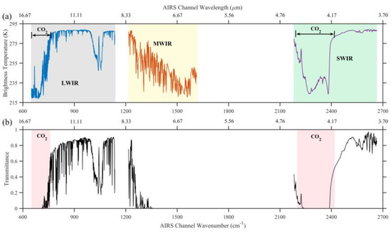
Figure 1.
The simulated (a) brightness temperature (K) and (b) transmittance for Atmospheric Infrared Sounder (AIRS) by the radiative transfer model CRTM with the U.S standard atmospheric profile. LWIR, MWIR, and SWIR represent longwave infrared, midwave infrared, and shortwave infrared, respectively.
2.2. CALIOP Observations
The Cloud-Aerosol Lidar and Infrared Pathfinder Satellite Observations (CALIPSO) mission, developed as a collaboration between the National Aeronautics and Space Administration (NASA) from the USA and Centre National d’ Études Spatiales (CNES) from France, provides a new pathway to observe the aerosols and clouds over the Earth [39]. The CALIPSO was launched in April 2006 with the CloudSat satellite and as a part of the A-Train constellation [40]. The range of the global coverage of CALIPSO is from 82°S to 82°N and the revisit time is 16 days [41]. CALIPSO carries an elastic backscatter lidar named CALIOP, which provides profiles and properties of cloud and aerosol particles. CALIOP, as an active sensor, observes the earth during the daytime for the equator-crossing time at 13: 30 and nighttime at 01: 30, respectively [42]. The accurate cloud heights can be obtained from the total backscatter measurements of CALIOP. The discriminate ice clouds and water clouds are derived from the depolarization measurements [43]. The CALIOP has three different horizontal resolutions in level-2 cloud-layer products, that is, 333 m, 1 km, and 1.67 km. Since the 333 m resolution product can only be used up to 8.3 km above sea level [44], the 1 km resolution product, whose vertical range is up to 20.2 km, was employed to collocate AIRS L1B data for evaluation and validation in this study. The CALIOP 1 km cloud products in four months from four seasons— from January 1 to January 31, April 16 to May 15, July 16 to August 15, and October 16 to November 15 in 2016—were used to train the thresholds of the ice cloud detection to reduce the effect of seasonal variation. Further, the optical depth from 5 km layer product was used to assess the performance of ice cloud detection with different optical depth.
2.3. The Community Radiative Transfer Model
The CRTM, developed at the Joint Center for Satellite Data Assimilation (JCSDA), is a fast radiative transfer model used to simulate radiance [45,46]. Microwave and infrared spectrums are covered for most satellite sensors in the CRTM. The radiative transfer problem in CRTM is mainly divided into various components, for instance, gaseous absorption, surface emissivity/reflectivity, aerosol absorption/scattering, and cloud absorption/scattering components. The inputs include some atmospheric profiles (e.g., pressure, temperature, water vapors, and ozone) and surface variables such as surface type and surface temperature [47]. The optional input data contain cloud and aerosol variables (e.g., cloud water content and cloud effective radius). There are six cloud types, including ice, water, rain, snow, graupel, and hail, in the CRTM. During the process of simulation in the IR spectral region, there are three surface emissivity or reflectivity models used for land and two models for water. Spherical liquid water clouds are assumed satisfying the Mie scattering theory and modified gamma size distribution [48]. However, ice cloud particles are supposed to be non-spherical hexagonal columns and with a gamma size distribution in the IR spectral area [47]. In this study, the CRTM was employed to simulate the weighting function of AIRS channels.
3. Methods
3.1. Collocation between AIRS and CALIOP
Collocation of the two instruments is needed in order to find the same location on the Earth at the same time. AIRS onboard Aqua and CALIPSO belongs to the A-Train constellation. CALIPSO lags behind Aqua by about 100 s [39], and the time difference is negligible. The quasi-elliptical approach [49] was employed to collocate CALIOP Level 2 cloud products with the AIRS level 1B. CALIOP is defined as the “slave” sensor and AIRS as the “master” sensor. The “slave” profiles from CALIOP should be put onto the master’s FOVs. Figure 2 shows an example of an AIRS swath and CALIOP track. The collocated FOVs are mostly located at the AIRS near-nadir position, therefore, the collocated FOV around near-nadir measurements are considered as the accurate observation in this study.
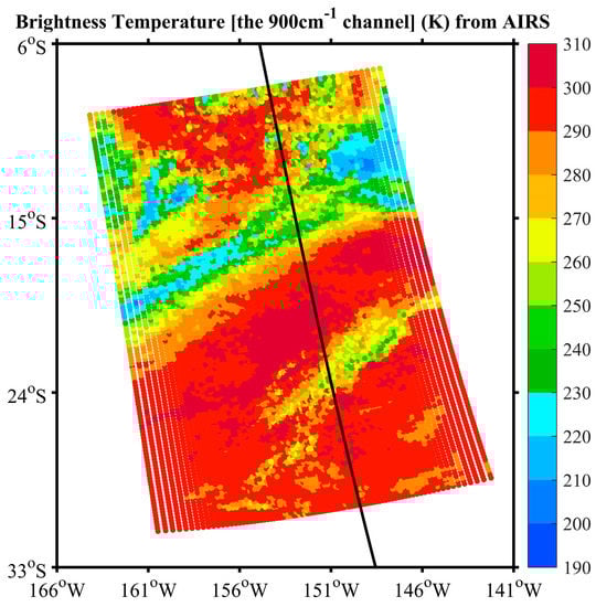
Figure 2.
An example of an AIRS swath with a brightness temperature from the 900 cm−1 channel collocating with the Cloud-Aerosol Lidar with Orthogonal Polarization (CALIOP) orbit track (black line).
In the CALIOP 1 km cloud layer product, CALIOP profiles have four categories: clear, single-layer clouds, multi-layer clouds, and heterogeneous clouds in the “Feature Classification Flag” in the cloud product. There are four quality levels for the four categories as well, which are “None”, “Low”, “Medium”, and “High”. Only the “Medium” and “High” quality of CALIOP profiles were considered in this paper. In each CALIOP profile, there are three cloud phases: ice (including randomly oriented and horizontally oriented), water, and unknown. Unknown cloud phases are more complex and we did not consider them. Meanwhile, the CALIOP profiles of “low” confidence are excluded because the profiles with “low” confidence phase are based on the temperature in the CALIOP retrieval and might mistakenly classify the profiles of water phase as ice phase or ice phase as the water phase [50]. The ice cloud phase for the AIRS FOVs was defined whenever the fraction of CALIOP ice clouds profiles was equal to or above 80%. When the percentage of CALIOP water clouds profiles was equal to or above 80% in AIRS FOVs, the AIRS FOVs were defined as water cloud phase; clear sky profiles that occupied the number equal to or above 80% in AIRS FOV were defined as clear sky. Finally, when different cloud phases were seen in the AIRS FOV and the percentage of each of these phases (i.e., the ratio of ice clouds) was less than 80%, the AIRS FOV was defined as a “mixed phase”. It is noted that AIRS could only detect the uppermost layer of clouds; therefore, the first layer of the cloud’s top pressure for CALIOP profiles was averaged within the AIRS FOV. The number of collocated AIRS FOVs was approximately 2.4 million between the 60°S and 60°N region in four seasons, and the detailed numbers are shown in Table 1.

Table 1.
Number of collocated AIRS fields of view for clear sky and ice, water, and mixed cloud phases.
3.2. Evaluation Method
The performance of cloud detection in different layers was evaluated by categorical scores. The probability of detection (POD), also called the hit rate, is sensitive to the number of clouds detected correctly by the Cloud Emission and Scattering Index (CESI). Larger POD values represent better cloud detection. However, the POD ignores false alarms. To conduct a fair comparison of the PODs among different pairs of CESI values, the false alarm rate (FAR) was introduced. Generally, the FAR is defined as the ratio of false alarms to the total number of Cloud detections by CESI (Hits and False alarms). However, in this study, the FAR, also known as the probability of false detection (POFD), was the fraction of false alarms to the total number of no–cloud detections by CALIOP. The FAR is sensitive to false alarms and was used in conjunction with POD. Both conceptual and geometrical foundations were provided by POD and FAR for our detection approach.
The POD and FAR are defined as follows:
where definitions of a, b, c, and d are shown in Table 2.
Table 2.
Cloud- /no–cloud detection by CALIOP and cloud emission and scattering index (CESI).
The Heike Skill Score (HSS) measures the fraction of the correct cloud detections method after eliminating the accuracy of detections that would be corrected because of random chance. It has been widely used to evaluate cloud detection and weather forecast [51,52]. After developing the cloud detection scheme, the exact thresholds of the algorithm for ice cloud detection should be obtained. The HSS was used to obtain the thresholds of the ice clouds detection scheme and is defined as:
The proportion correct by chance can be expressed as:
Equation (2) can be simply expressed as:
where a, b, c, and d are defined in Table 2. The range of HSS is from −1 to 1.
4. A Cloud Detection Method by Combining LWIR and SWIR CO2 Bands
There are four steps to derive cloud detection. These steps are listed below, (1) calculating the weighting function peak (WFP) altitudes of LWIR and SWIR channels; (2) determining the cut-off pressure (COP) level; (3) extracting strongly correlated pairs; (4) establishing the cloud emission and scattering index. The above three steps are used to pair LWIR and SWIR channels and the fourth step is used to establish the cloud detection based on the paired LWIR and SWIR channels.
4.1. Weighting Function Peak Altitude of LWIR and SWIR Channels
The weighting functions (WFs) for LWIR and SWIR are calculated by CRTM using the U.S. standard profile. The WF is defined as follows:
where is the weighting function of the channel , is the transmittance at the kth layer, is the atmospheric pressure at kth layer, is the optical depth of the kth layer, and is the satellite zenith angle. The longwave infrared (LWIR) and shortwave infrared (SWIR) channels are chosen from 670–760 cm−1 and 2200–2400 cm−1, respectively. The WFP altitudes should be from the surface to tropopause which was around 150 hPa and is shown in Figure 3a.
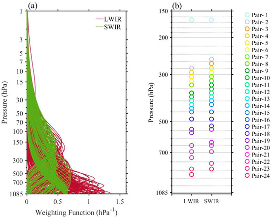
Figure 3.
(a) The weighting function of 204 LWIR and 116 SWIR channels whose weighting function peaks were located from the surface to 150 hPa. (b) The weighting function (WF) peak altitude for paired LWIR and SWIR channels.
4.2. Finding the Cut-Off Pressure Level
In the first step, some channels with the same peak WF altitude exist, but the shapes of WFs are different. As shown in Figure 4, the WFP altitudes of the Ch 224 (713.61 cm−1) and Ch 297 (734.77 cm−1) are the same (dashed black line). However, the WF structure of Ch 297 is “broad” while Ch 224 is “narrow”. To find the level of cloud sensitivity, the cut-off pressure level was introduced [53]. The COP level was set based on the WF structure. This means that when the top of a cloud exists above the COP level, this channel is considered to be contaminated by clouds. According to the definition of COP altitude in Carrier et al. [53], the COP altitude is defined that the integrated emission above the COP level is 4 times that from the COP level below. The COP level was set from the near-surface level to the top of atmosphere and calculate iteratively COP level until met the function as follows,
where is the weighting function, which represents the transmittance at vertical kth layer at channel , is the integrated emission from the surface to the altitude of COP, and is the integrated emission above the COP altitude. The COP levels above the WF peak height and that exist at the surface are excluded. In Figure 4, the COP altitude of narrow channel (Ch 224, dashed red line, at~506 hPa) is higher than that of the broad channel (Ch 297, dashed green line, at ~650 hPa), indicating that WFs with “broad” structures receive radiance from a deeper atmospheric layer. The received radiances for WFs with “narrow” structures are from a shallower atmospheric layer.
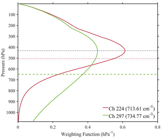
Figure 4.
The cut-off pressure (COP) altitude and the WF profiles for Ch 224 (713.61 cm−1) and Ch 297 (734.77 cm−1). The WF profiles of Ch 224 and Ch 297 are indicated in red and green solid line. The COP levels of Ch 224 and Ch 297 are shown in red and green dashed line. The black dashed line represents the WFP altitude of these two channels.
4.3. Extracting Strongly Correlated Pairs
After calculating the WFP and COP altitudes for LWIR and SWIR channels (in Section 4.1 and Section 4.2), there were 160 LWIR and 78 SWIR channels that met the altitudes of WFP and COP. As reported by Kahn and Teixierra [54], the atmospheric information (such as temperature and water vapor) is varied in the different levels of atmosphere. In order to minimize the variation of atmosphere, the altitude of WFP and COP for one LWIR channel should be equal to or less than two pressure levels of those for SWIR channel and the pressure levels are calculated by using CRTM model. Therefore, the number of LWIR channels that met the requirements of the SWIR channel could be more than one, and vice versa. The final pairs between LWIR and SWIR channels are determined by their correlation coefficient. To avoid the influence of the surface emissivity and sea ice located in the Antarctic and Arctic, we considered the area from 60°S and 60°N. In this section, the clear sky FOVs are derived from AIRS Level 2 IR-only products. When the effective cloud fraction (represented by CldFrcStd) from AIRS Level 2 products was equal to 0, the AIRS FOVs was considered as clear-sky FOVs. Since SWIR channels are affected by solar radiation in the daytime, clear sky FOVs was separated into daytime and nighttime. The number of clear-sky AIRS FOVs between 60°S and 60°N were 2 211 648, 2 158 519, and 4 370 167 for daytime, nighttime and day/night time, respectively. A two spectra cross method was employed to calculate the correlation coefficient [55,56].
where is the correlation coefficient; and stand for the LWIR and SWIR channels, respectively; and D are the clear-sky brightness temperature of the mean and standard deviation for each channel. is the number of total clear-sky AIRS FOVs. Only strong correlations between LWIR and SWIR channels were considered in this study; therefore, we selected the maximum correlation coefficients that were equal to or greater than 0.7 (significance level < 0.01). Figure 5 shows the correlation coefficient between the paired LWIR and SWIR channels. The paired LWIR channels were located from 700 m−1 to 750 cm−1 whereas SWIR channels accumulated in two regions, 2220 m−1 to 2280 m−1 and 2380 m−1 to 2400 cm−1.
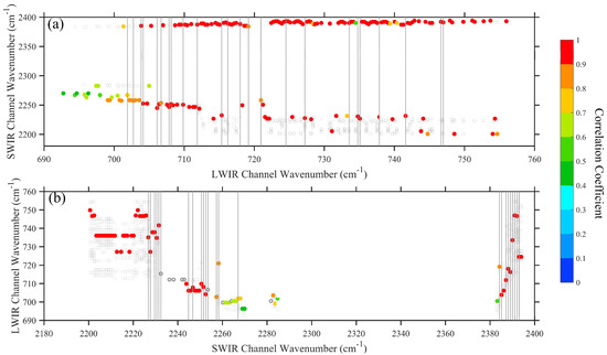
Figure 5.
The correlation coefficient between paired LWIR (a) and SWIR (b) channels. Grey circles represent the correlation coefficient and colored symbols indicate the maximum correlation coefficient between LWIR and SWIR channels. The final twenty-four (24) pairs between LWIR and SWIR channels are represented by grey line.
After above three steps, there were a total of twenty-four (24) pairs, and their channel number, wavenumbers, peak WF altitudes, cut-off pressure levels, and correlation coefficients are shown in Table 3. Figure 3b presents the WFPs of paired LWIR and SWIR channels. As seen from Figure 3b, the WFPs of LWIR channels and their corresponding SWIR channels are located in similar altitudes so that they can be effectively used to detect clouds in the different levels of the atmosphere.
Table 3.
The paired twenty-four (24) LWIR and SWIR channels including channel number, wavenumber, peak WF altitude, cut-off pressure levels, and correlation coefficients.
4.4. The Cloud Emission and Scattering Index
After the three steps above, the correspondence between the LWIR and SWIR channels was one- to- one. To find the relationship between LWIR and paired SWIR channel under clear sky, a linear regression can be established for each pair:
where BT is the observed brightness temperature for SWIR and LWIR channels. The subscript “i” represents the number of pairs. The regression coefficients α and β are derived from the least squares in the minimizing cost function as follows:
where the subscript “j” is the number of the clear sky FOVs. When we obtain the regression coefficients α and β, a cloud emission and scattering index (CESI) can be defined as follows [24,57]:
Some research studies show that when clouds top pressure is above the WFP altitude, it has more influence on the observed radiances while clouds top pressure is below the WFP altitude, the effect is smaller [58,59]. Based on the WFP altitude, a total of twenty-four (24) pairs of CESI were divided into fifteen (15), six (6), and three (3) pairs for upper, middle, and lower troposphere cloud detection, respectively and shown in Table 3. Since the observed brightness temperature from AIRS is affected by scan-dependent features and the relationship between LWIR and SWIR channels varies with viewing angle, a linear regression was made for 90 AIRS FOVs to reduce this variation. Figure 6 represents scatterplots of brightness temperatures of LWIR 218 and SWIR 2108 channels (WFP ~433 hPa) at nadir (FOV 45) and off-nadir (FOV 1) FOVs. As can be seen in the figure, whether in daytime (Figure 6a,b) or nighttime (Figure 6c,d), slopes exceeding unity are seen when the value of SWIR BT is plotted against that of LWIR BT. This indicates that the range of SWIR brightness temperature was wider than that of LWIR in the regression training data. Han et al. [43] found the same results. They also showed that the variability and slope were greater when using observations rather than using model simulations. The difference in regression between at nadir and off-nadir FOVs was based on the observed brightness temperature. This clearly showed that the brightness temperature at nadir was higher than at off-nadir positions in both LWIR 218 and SWIR 2108 channels. However, the difference in regression between day and night was not obvious in Pair-15.
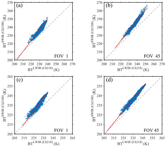
Figure 6.
Scatterplot of brightness temperature of SWIR 2108 channel and paired LWIR 218 channel at the nadir (b,d) and off-nadir (a,c) FOVs in the daytime (a,b) and nighttime (b,d) under the clear sky condition.
Figure 7 shows the regression coefficients slope () and intercept () in the ascending orbit (Figure 7a,b) and descending orbit (Figure 7c,d). It shows that the regression coefficients had symmetric variation with AIRS FOVS. The large slope () value was mostly at nadir FOVs and small values were at the off-nadir FOVs. The regression coefficients were similar for pairs with high WFP altitudes in daytime and nighttime, however, there were some differences in middle and lower WFP pairs.
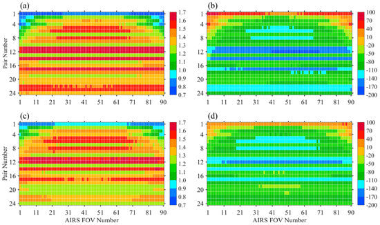
Figure 7.
Regression coefficients for slope (α) and intercept (β) for 90 FOVs of the 24 pairs. The x-axis is the 90 AIRS FOV number and the y-axis is pair number. (a,b) are in the ascending orbit (daytime) and (c,d) are in the descending orbit (nighttime). The slope (α) and intercept (β) are dimensionless.
5. Evaluation and Validation
5.1. Limb Correction
Since AIRS is a cross-track sensor, the observed brightness temperature was affected by the latitudinal and scan-dependent positions, and the calculated CESIs were affected as well. Some studies corrected the limb effect by two steps [60,61,62]. The first step is calculating the bias of each FOV and subtracting the nadir bias to correct the scan-dependent bias of variables (e.g., brightness temperature). The function is shown as follows,
where is the bias of different FOVs, is the viewing angle, and the subscript “i” represents the number of FOVs.
The second step was correcting latitudinal biases by calculating the variable values at nadir in some grid latitudinal band. The function can be defined as follows,
where is the bias of latitudinal, represents different latitudinal bands and the subscript represents every 2° latitudinal band. Then, the variables after limb correction were derived by subtracting the scan-dependent and latitudinal biases from the variables before limb correction.
Li and Zou [63] pointed out that the bias in brightness temperature varied with the latitude and scan position simultaneously, and it had a clear seasonal variation. Therefore, the AIRS clear-sky data in each FOV are separated into four seasons (represented by April, July, October, and December) in both day and night. Limb effects were corrected by using data from half a month before obtaining the thresholds of ice clouds detection. Detailed AIRS clear-sky data were from December 16 to December 31 for winter, from April 1 to April 15 for spring, from July 1st to July 15th for summer, and from October 1 to October 15 for autumn. The bias of latitude and san position for CESI can be shown as follows,
where is the viewing angle, the subscript (1-90) represents the number of AIRS FOVs, represents different latitudinal bands, and the subscript (1-60) stands for every 2° latitudinal band.
Figure 8 presents the bias of Pair-4 CESI averaged in every 2° latitudinal band and at 90 FOVs from April 1 to 15, 2016. Figure 9 shows the spatial distribution of Pair-4 CESI (WFP~287 hPa) before and after limb effect adjustment on May 20. Shown in Figure 9a, limb brightening was the most extreme in the tropics, and the cloud pattern was not obvious before limb correction. The Pair-4 CESI after limb correction, conversely, reflected the cloud features clearly in the tropics (Figure 9b).
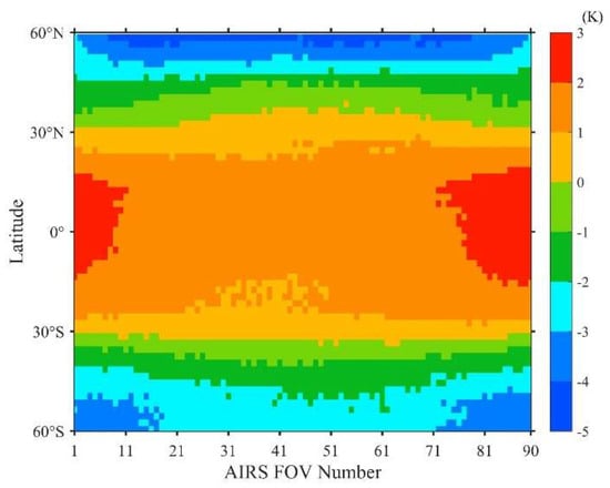
Figure 8.
The Pair-4 CESI (WFP~287 hPa) averaged in every 2° latitudinal band and at 90 FOVs under clear sky conditions. Data were measured in the daytime from April 1 to 15, 2016.
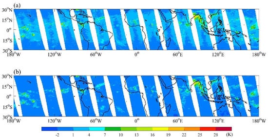
Figure 9.
Spatial distribution of Pair-4 CESI (WFP~287 hPa) from the ascending node between 30°S and 30°N on May 20, 2016 (a) before and (b) after limb effect corrections.
5.2. Evaluating and Obtaining the Thresholds of CESI Pairs
Collocated data between CALIOP 1 km cloud products and AIRS L1B from May 16 to May 23 in 2017 is used to evaluate the performance of CESI. The total cloudy and clear-sky numbers in this period were 60,146 and 21,532 for daytime. Ice clouds, water, and mixed clouds are 15,399, 33,527, and 11,220, respectively. In the nighttime, the cloudy and clear sky were 60,088 and 18,365 AIRS FOVs. The ice, water, and mixed cloud numbers were 15,862, 30,698, and 13,528. Pair-8 (WFP~330 hPa) in the upper, Pair-19 (WFP~555hPa) in the middle, and Pair-24 (WFP~866 hPa) in the lower troposphere are shown as examples. To characterize the distribution of CESI in detecting different cloud phase scenes, histograms of three pairs for clear sky, ice cloud, water cloud, and mixed cloud scenes from May 16 to May 23 in 2017 are shown in Figure 10. Generally, the clear sky distribution was around 0 K in both day and night for Pair-8, Pair-19, and Pair-24. This indicates that the derived CESIs were reasonable under the clear sky. The histogram of water clouds mostly overlapped with clear sky. This is because the observed brightness temperatures of water clouds are from the emission of the cloud top, and the emissivity of the cloud top for LWIR and SWIR was similar for thick water clouds. Conversely, for the ice clouds, the brightness temperatures of SWIR were larger than LWIR because of the difference in emissivity and scattering characteristics. The histogram of the mixed phase included ice clouds and water clouds. Comparing to the higher WFP pairs (i.e., Pair-8), the sensitivity to ice clouds was stronger in lower WFP pairs (i.e., Pair-24). Additionally, CESI values were larger in the daytime than at nighttime because of solar radiation in the shortwave channel.
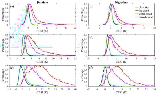
Figure 10.
Histogram of the CESI for clear sky, ice cloud, water cloud, and mixed cloud scenes in daytime (a,c,e) and nighttime (b,d,f) over 60°S and 60°N from May 16 to May 23 in 2017. (a,b) are Pair-8 (WFP~330 hPa), (c,d) are Pair-19 (WFP~555hPa), and (e,f) are Pair-24 (WFP~866 hPa). All histograms are scaled by the max value and shown as a percentage.
Figure 11 shows the POD and FAR variation with different CESI thresholds for Pair-8 (WFP~330 hPa), Pair-19 (WFP~555 hPa), and Pair-24(WFP~866 hPa) from May 16 to May 23 in 2017. The POD and FAR values varied with different CESI thresholds from −10 to 50 K. The performance of ice cloud detection was the best among the cloud phases, while it was unable to detect water clouds in both day and night. To minimize the FAR values, we assumed FAR values were at 0.1. The POD values of ice clouds were 0.63, 0.71, and 0.73 for Pair-8, Pair-19, and Pair-24 in the daytime, respectively. One of the reasons is that some ice clouds located between 330 hPa and 555 hPa could not be detected by Pair-8. The ice clouds detected for Pair-19 were similar to Pair-24. Furthermore, the POD values of ice clouds were 0.46, 0.62, and 0.7 in the nighttime. For detecting water clouds, whether in daytime or nighttime, the POD values of the three pairs are around 0 when the FAR values were at 0.1. The POD values of mixed-phase clouds in the daytime are 0.43, 0.20, and 0.12 for Pair-8, Pair-19, and Pair-24, respectively. It is noted that the POD values of mixed-phase clouds in Pair-8 were highest among the three pairs. The mixed clouds included water clouds and ice clouds. CESIs are sensitive to ice clouds but insensitive to water clouds. Some sample data of mixed clouds include multi-layer clouds with ice clouds and water clouds. The high ice clouds can be detected by Pair-8, but the altitudes of low water clouds were lower than Pair-8 WFP. Therefore, the POD of mixed phase for Pair-8 was highest. In the nighttime, the POD of the mixed-phase clouds was around 0.2 at a value of 0.1 of FAR. Three pairs of CESIs in different layers were sensitive to ice clouds but were unable to detect water and mixed-phase clouds.
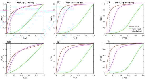
Figure 11.
Probability of detection (POD) and false alarm rate (FAR) at different CESI thresholds from −10 to 50 K for Pair-8, Pair-19, and Pair-24 in the daytime (a–c) and nighttime (d–f) from May 16 to May 23 in 2017.The gray dash lines represents the FAR value at 0.1.
Collocated data in four seasons in 2016 were employed to obtain the thresholds of CESI in three pairs. Categorical scores of HSS, POD, and FAR were calculated as a function of the CESI threshold in 0.1 K intervals. The three HSS, POD, and FAR pairs are shown in Figure 12. The CESI thresholds are derived from the corresponding index of the highest HSS score.
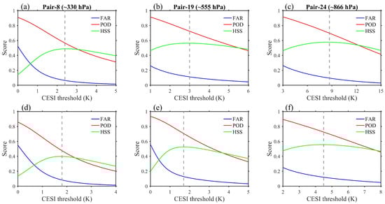
Figure 12.
CESI categorical scores as a function of the cloud threshold evaluated by CALIOP for different pairs during the day (a–c) and night (d–f).
The highest HSS values were 0.49, 0.56, and 0.58 in the daytime and 0.4, 0.53, and 0.56 in the nighttime. Correspondingly, the POD values were 0.55, 0.72, and 0.7 in the daytime and 0.4, 0.7, and 0.72 in the nighttime for Pair-8, Pair-19, and Pair-24, respectively. At the highest HSS values, the corresponding FAR values were 0.06, 0.11, and 0.1 in the daytime and 0.09, 0.13, and 0.12 in the nighttime. The results of the thresholds of CESI were 2.4 K, 3 K, and 8.7 K in the daytime and 1.7 K, 1.7 K, and 4.4 K in the nighttime for Pair-8, Pair-19, and Pair-24, respectively. Generally, the thresholds increased with the WFP pairs.
5.3. Validation
The cloud top pressure and cloud phase from CALIOP between May 16 and May 23 in 2017 were employed to validate Pair-8, Pair-19, and Pair-24 with thresholds of 2.4 K, 3 K, and 8.7 K in the daytime and 1.7 K, 1.7K, and 4.4 K in the nighttime for ice cloud detection. As shown in Figure 13, the HSS values were 0.47, 0.58, and 0.59 in the daytime and 0.38, 0.54, and 0.58 in the nighttime. The HSS values in both day and night had differences between 0.01~0.02 (within 5%), indicating that the values were close to those assessment and the performance of these three pairs’ thresholds was relatively good (Figure 12). Further, the POD values were 0.47, 0.76, and 0.72 in the daytime and 0.47, 0.77, and 0.77 in the nighttime. Correspondingly, the FAR values were 0.05, 0.12, and 0.1 in the daytime and 0.11, 0.15, and 0.13 in the nighttime. For Pair-8, the POD values and FAR values were slightly less than those in the assessment; however, for Pair-19 and Pair-24, the POD and FAR values were slightly larger than those in assessment. It is reasonable that the values of POD and FAR increased and decreased simultaneously.
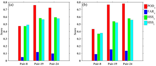
Figure 13.
The validation value of POD, FAR, and Heike Skill Score (HSS) with subscript “v” and the training value of HSS with subscript “t” for the Pair-8, Pair-19, and Pair-24 with 2.4 K, 3 K, and 8.7 K in the daytime (a) and 1.7 K, 1.7K, and 4.4 K in the nighttime (b) from May 16 to May 23 in 2017.
5.4. Evaluation of CESI Ice Clouds Detection by CALIOP Optical Depth
In Section 5.2 and Section 5.3, we obtain and validate the thresholds of ice clouds in Pair-8, Pair-19, and Pair-24 by CALIOP data. Further, in order to evaluate the ice cloud detection by CESI for the three pairs, ice clouds optical depth from CALIOP Level 2 5 km layer product was used to calculate the optical depth of collocated ice clouds FOVs in Section 5.1. Figure 14 shows the frequency of detected and missed ice clouds with optical depth for the three pairs. Both in daytime and nighttime, the frequency of missed ice clouds with optical depth in the range of 0 and 0.6 is higher than detected ice clouds. For Pair-8, the frequency of detected ice clouds is consistent with missed ice clouds. However, the frequency of detected ice clouds is larger than that of missed ice clouds for Pair-19 and Pair-24 when the optical depth of ice clouds is larger than 0.6. For Pair-19 and Pair-24, when optical depth is between 1 and 5, the frequency of detected ice clouds is more than that of missed ice clouds in the daytime (Figure 14c,e). Further, the frequency of detected ice clouds with optical depth between 6 and 8 increases in the nighttime (Figure 14b,d,f).
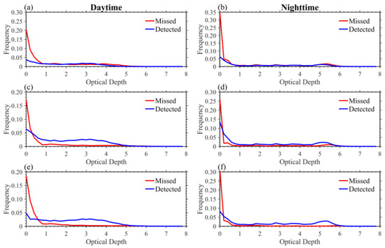
Figure 14.
The frequency of detected and missed ice clouds for Pair-8 (a,b), Pair-19 (c,d) and Pair-24 (e,f) from May 16 to May 23, 2017 in the daytime (a,c,e) and nighttime (b,d,f).
Based on the histogram of detected and missed ice clouds by CESI, in order to further examine the ice clouds detection of CESI for different ranges of ice clouds optical depth, ice clouds detected by CALIOP from May 16 to May 23 are classified into four categories according to optical depth () values. The ice clouds are classified into four categories and types are list as follows. (1) sub-visual ice clouds (); (2) thin ice clouds (); (3) opaque ice clouds (); (4) thick ice clouds () according to the Sassen and Cho classification method [64]. Some other studies also use the similar classification method to study the distribution and properties of different types of ice clouds [2,3,65].
Figure 15 and Figure 16 show the occurrence frequency of ice clouds with different optical depths from May 16 to May 23, 2017. The sub-visual ice clouds () are most located in the tropical areas and the most occurrence frequency of sub-visual ice clouds is around 45%, which locate in the Pacific warm pool (in Figure 15a). The number of thin ice clouds () is larger than sub-visual ice clouds and thin ice clouds mainly occur in tropical and 50°N areas. The number of opaque ice clouds () is largest for four categories. The occurrence areas of opaque ice clouds are mainly in the tropical areas including the Indian Ocean and the South America. The number of opaque ice clouds in mid-latitude is most among the four categories. For the thick ice clouds (in Figure 15d), the distribution is similar for thin ice clouds, but the number is smaller than thin ice clouds. In the nighttime, the number and the occurrence frequency of sub-visual and thin ice clouds are more than those in the daytime (in Figure 16a). This is because the height of optically thin ice clouds (i.e., cirrus) increases in the nighttime [66]. Also, both occurrence frequency and the number for opaque ice clouds are highest among the four types of ice clouds in the nighttime. Further, the occurrence frequency of thick ice clouds is larger than those in the daytime, especially in the 50°S regions.
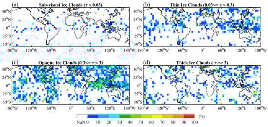
Figure 15.
The occurrence frequency of ice clouds with different optical depth within 5° × 5°grid boxes in the ascending orbit from May 16 to May 23, 2017. The data are based on collocated CALIOP 5-km cloud layer data and CESI data. (a) Sub-visual ice clouds (); (b) thin ice clouds (); (c) opaque ice clouds (); (d) thick ice clouds ().
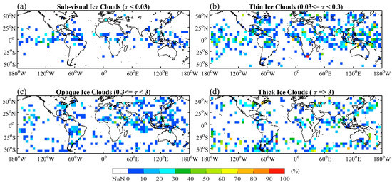
Figure 16.
Same as Figure 15 but in the descending nodes.
Figure 17, Figure 18 and Figure 19 represent the performance of four categories of ice clouds detection by Pair-8, Pair-19, and Pair-24, respectively. The distribution of ice clouds with different optical depth is similar in Figure 14 and Figure 15. The number of opaque ice clouds is the most and sub-visual is the least. As shown in Figure 17a–d, most ice clouds with optical depth less than 0.3 are missing detection by Pair-8, especially for sub-visual ice clouds. For opaque and thick ice clouds, Pair-8 can detect them located in the tropical areas, especially in the mainly ice cloud occurrence regions (the Pacific warm pool, center Africa, and South America) but fail to detect opaque ice clouds located in the mid-latitude. This is because of the ice clouds height are high in the tropical region and lower in the mid-latitude [66]. When ice cloud top pressure of ice clouds above 555 hPa, Pair-19 detects more thin ice clouds than Pair-8 (in Figure 18c,d) and still fail to detect some thin ice clouds located in the mid-latitude. For the opaque and thick ice clouds, most of them can be detected by Pair-19 in both daytime and nighttime. As shown in Figure 19a–d, most sub-visual and thin ice clouds are unable to be detected by Pair-24, especially in the mid-latitude. However, most opaque and thick ice clouds can be detected by Pair-24. Therefore, CESI has the ability to detect ice clouds with optical depth larger than 0.3 but it is not sensitive to sub-visual and thin ice clouds. These results are same as other passive sensors [67,68].
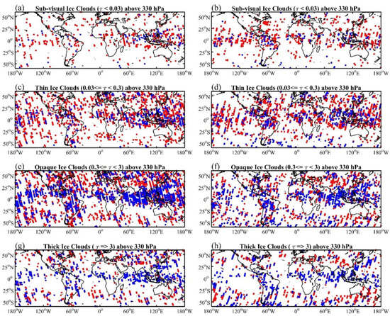
Figure 17.
Ice cloud top pressure above 330 hPa detected by Pair-8 for different categories from May 16 to May 23, 2017. The left column is in the ascending orbit and the right column is in the descending orbit. (a,b) are the sub-visual ice clouds (); (c,d) are the thin ice clouds (); (e,f) are the opaque ice clouds (); (g,h) are the thick ice clouds (). Blue dots denote detected and red dots denote missed.
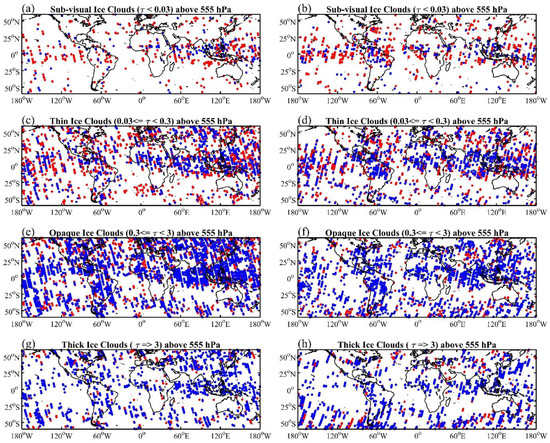
Figure 18.
Same as Figure 17 but for the ice clouds top pressure above 555 hPa and detected by Pair-19.
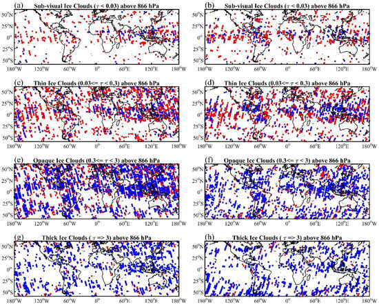
Figure 19.
Same as Figure 17 but for the ice clouds top pressure above 866 hPa and detected by Pair-24.
6. Discussion
This study was based on Lin17’s cloud detection scheme named Cloud Emission and Scattering Index (CESI), by using dual CO2 bands in the Cross-track Infrared Sensor (CrIS) [24]. In their research, simulated data were used to derive CESI, without separately considering daytime and nighttime and deriving the thresholds of cloud detection. This algorithm is based on the theory that the different characteristics in emission and scattering of ice clouds perceived by longwave and shortwave CO2 absorption bands. Moreover, they pointed out that when thin ice clouds existed, the CESI values were positive, whereas the CESI values were negative when thick clouds existed. However, the accurate thresholds of ice clouds had not been provided in their research for each pair. In Wang19, the thin cirrus from VIIRS cloud mask product was collocated with CESI to assess the thin cirrus detection of CESI from Lin17 and low WFP pairs were combined by using linear discriminant analysis to improve cirrus detection. The results showed that the POD of thin cirrus was 0.69 for the pair with WFP~891 hPa when FAR set at 0.1. Three low WFP pairs were combined and the POD values increased to 0.77 and 0.75 with the FAR of 0.1 in the daytime and nighttime, respectively. However, there are some drawbacks from Wang19. In the VIIRS cloud mask product, the thin cirrus in the daytime was retrieved by the 1.38 μm channel in the daytime. The performance of thin cirrus was affected by elevated surfaces, dry atmospheric conditions, and high albedo surfaces [37]. This would lead to some mistakes in the process of cirrus evaluation. Additionally, the cloud top pressures of cirrus had not been considered in Wang19 because the cloud top pressures information was not available in the VIIRS cloud mask product. In this paper, real observation data were employed to derive CESI for AIRS and separated daytime and nighttime because Kahn et al. [28] pointed out that there is a difference in detecting clouds in the daytime and nighttime. Further, the active lidar sensor CALIOP was more accurate in detecting clouds than passive satellite sensors, especially for optically thin cirrus [69]. The CALIOP was employed to collocate with CESI to derive the thresholds of ice clouds according to the highest evaluation score of HSS. The POD values of ice clouds were 0.72 and 0.77 for Pair-24 (WFP~866 hPa) with FAR of 0.1 and 0.13 in the daytime and nighttime, respectively. The POD values were larger than the individual CESI but less than the improvement values in Wang19. This is because the improvement of ice clouds detection was most often located in the mid-latitude areas. Further, the ice cloud optical depth from CALIOP was considered in this study, which was lack in Lin17 and Wang19. AIRS cloud product has been evaluated by using CALIOP product, which shows that the POD values is over 0.9 with FAR values around 0.1 [44] while the POD is about 0.77 for the Pair-24 in this study. The difference mainly comes from the different algorithm. Window channels were used to detect ice clouds in AIRS cloud product because there is less effect on the absorption gas for window channels [28]. However, window channels could not detect ice cloud directly in certain vertical atmospheric layers and would be affected by surface type.
Despite the improvements made by this paper algorithm, there are several limitations of CESI and the thresholds of ice clouds detection in this paper. First, the cloud detection scheme developed by AIRS fail to detect some sub-visual () and thin () ice clouds. One of the reasons is from the passive sensor limitations [68,70], of which the viewing angle, contrast, and molecular scattering problems may affect the instruments’ ability to detect clouds [64,67]. The second limitation could be due to the collocation between CALIOP and AIRS. The AIRS FOVs is around 13.5 km at the nadir while the spatial of CALIOP profiles is around 1 km. Even we selected the percentage of ice cloud profiles from CALIOP in each AIRS FOV is equal to or larger than 80%, the inhomogeneous ice clouds still exist because of the track orbit of the CALIOP and AIRS observations. In the assessment of CESI for ice clouds, water clouds, mixed phase clouds, and clear sky, the CESI values of ice clouds is largest. Therefore, when ice clouds together with other conditions (water clouds, mixed phase clouds, and clear sky), the obtained threshold of ice clouds would be underestimated and it is possible to unable to detect the inhomogeneous ice clouds. Another potential problem for this ice cloud detection algorithm could be from CO2 concentration effect [71]. As reported in this study, the authors did the sensitivity experiments and showed that the thin cloud frequency in the high altitude was influenced by 5-10 ppm CO2 variations, typically for seasonal and regional variation. In this algorithm, AIRS and CALIOP data from four months (January, April, July, and October) were used to reduce the effect of CO2 and cloud seasonal variation. However, the uncertain CO2 rising level may have an impact on using CO2 bands to detect clouds. Additionally, the CESI only could detect single-layer ice clouds. Furthermore, the ice clouds with the thin optical depth would give rise to the bias rising in the data assimilation procedure because the thin ice clouds would be considered as clear-sky then input to the model [24].
Based on the current limitations, some further studies could be done to improve the ice clouds detection. Due to the fact that the ice clouds located in the mid-latitude are not detected by CESI with high WFP altitude, the linear discriminant analysis and other CO2 channels could be combined to improve ice clouds detection based on Wang19.
7. Conclusions
Detecting ice clouds in specific atmospheric layers is still a challenge for infrared sensors. The paper [24] developed an algorithm to detect clouds in different layers by combining longwave (wavenumber from 670~760 cm−1) and shortwave (wavenumber from 2200~2400 cm−1) CO2 absorption bands from the Cross-Track Infrared Sounder (CrIS). This algorithm, named Cloud Emission and Scattering Index (CESI), is based on the theory that the difference in emission and scattering characteristics of clouds for longwave infrared (LWIR) and shortwave infrared (SWIR) CO2 channels. This study, based on Lin’s method, uses dual CO2 absorption bands of AIRS combined to detect ice clouds in different atmospheric layers. In our pairing process, we considered the weighting function peak (WFP) altitude, the cut-off pressure (COP) level, and the correlation coefficient. The observed brightness temperature (BT) was used instead of Lin’s simulation data, and daytime and nighttime were separated to establish the linear relationships. After that, we corrected the limb effect of CESI by calculating the latitudinal and seasonal bias in every 2° latitudinal band and at 90 FOVs under the clear sky. After limb correction, the CALIOP Level 2 cloud layer product was employed to collocate with AIRS CESI from May 16 to May 23, 2017, and the false alarm rate (FAR) and the probability of detection (POD) were applied to assess the performance of cloud detection. Finally, the thresholds of CESI for each pair in ice cloud detection were derived when the Heike Skill Score (HSS) is at the highest value.
A total of twenty-four (24) pairs of CESI were identified from the upper to lower troposphere. Pair-8 (WFP~330 hPa), Pair-19 (WFP~555 hPa), and Pair-24 (WFP~866 hPa) were selected to present as examples of pairing in the upper, middle, and lower troposphere, respectively. The results show that the POD values of ice clouds were 0.63, 0.71, and 0.73 for Pair-8, Pair-19, and Pair-24 in the daytime and 0.46, 0.62 and 0.7 in the nighttime, respectively, at FAR values of 0.1. However, the POD values were around 0.2 and below 0.05 for mixed and water cloud phases with FAR at 0.1. Therefore, CESI could detect ice clouds, but it was not very easy to identify water and mixed clouds. The thresholds of CESI were 2.4 K (1.7 K), 3 K (1.7 K), and 8.7 K (4.4 K) in the daytime (nighttime) for Pair-8, Pair-19, and Pair-24, respectively. Furthermore, the error of HSS values based on thresholds of ice clouds is between 0.01 and 0.02, indicating that the performance of ice cloud detection thresholds was relatively good. When evaluating the ice clouds detection with different optical depth from CALIOP, most of the ice clouds with optical depth that are less than 0.3 are not detected by CESI due to the passive sensor shortcomings. Moreover, Pair-8 failed to detect ice clouds located in the mid-latitude regions. It may be necessary to combine some other pairs with Pair-8 to improve the detection of ice clouds in the future.
Author Contributions
Conceptualization, L.W. and Y.Z.; methodology, L.W.; software, L.W., Z.N., J.X., W.C., and R.J.; validation, L.W. and C.L.; writing—original draft preparation, L.W.; writing—review and editing, L.W. and C.L.; supervision, Y.Z. and C.L.; funding acquisition, Y.Z. All authors have read and agreed to the published version of the manuscript.
Funding
This research was funded by the National Natural Science Foundation of China, grant number 41590873.
Conflicts of Interest
The authors declare no conflict of interest.
References
- Yang, P.; Liou, K.-N.; Bi, L.; Liu, C.; Yi, B.; Baum, B.A. On the radiative properties of ice clouds: Light scattering, remote sensing, and radiation parameterization. Adv. Atmos. Sci. 2015, 32, 32–63. [Google Scholar] [CrossRef]
- Lolli, S.; Campbell, J.R.; Lewis, J.R.; Gu, Y.; Marquis, J.W.; Chew, B.N.; Liew, S.-C.; Salinas, S.V.; Welton, E.J. Daytime top-of-the-atmosphere cirrus cloud radiative forcing properties at singapore. J. Appl. Meteorol. Clim. 2017, 56, 1249–1257. [Google Scholar] [CrossRef]
- Gouveia, D.A.; Barja, B.; Barbosa, H.M.; Seifert, P.; Baars, H.; Pauliquevis, T.; Artaxo, P. Optical and geometrical properties of cirrus clouds in Amazonia derived from 1 year of ground-based lidar measurements. Atmos. Chem. Phys. 2017, 17, 3619–3636. [Google Scholar] [CrossRef]
- Cutillo, L.; Amato, U.; Antoniadis, A.; Cuomo, V.; Serio, C. Cloud detection from multispectral satellite images. In Proceedings of the IEEE Gold Conference, Naples, Italy, 13–14 May 2004. [Google Scholar]
- McNally, A. A note on the occurrence of cloud in meteorologically sensitive areas and the implications for advanced infrared sounders. Q. J. R. Meteorol. Soc. A J. Atmos. Sci. Appl. Meteorol. Phys. Oceanogr. 2002, 128, 2551–2556. [Google Scholar] [CrossRef]
- Jedlovec, G. Automated detection of clouds in satellite imagery. Adv. Geosci. Remote Sens. 2009, 303–316. [Google Scholar] [CrossRef]
- Aumann, H.H.; Chahine, M.T.; Gautier, C.; Goldberg, M.D.; Kalnay, E.; McMillin, L.M.; Revercomb, H.; Rosenkranz, P.W.; Smith, W.L.; Staelin, D.H. AIRS/AMSU/HSB on the Aqua mission: Design, science objectives, data products, and processing systems. IEEE Trans. Geosci. Remote Sens. 2003, 41, 253–264. [Google Scholar] [CrossRef]
- Chahine, M.T.; Pagano, T.S.; Aumann, H.H.; Atlas, R.; Barnet, C.; Blaisdell, J.; Chen, L.; Divakarla, M.; Fetzer, E.J.; Goldberg, M. AIRS: Improving weather forecasting and providing new data on greenhouse gases. Bull. Am. Meteorol. Soc. 2006, 87, 911–926. [Google Scholar] [CrossRef]
- Le Marshall, J.; Jung, J.; Goldberg, M.; Barnet, C.; Wolf, W.; Derber, J.; Treadon, R.; Lord, S. Using cloudy AIRS fields of view in numerical weather prediction. Aust. Meteorol. Mag. 2008, 57, 249–254. [Google Scholar]
- Le Marshall, J.; Jung, J.; Derber, J.; Chahine, M.; Treadon, R.; Lord, S.J.; Goldberg, M.; Wolf, W.; Liu, H.C.; Joiner, J. Improving global analysis and forecasting with AIRS. Bull. Am. Meteorol. Soc. 2006, 87, 891–895. [Google Scholar] [CrossRef]
- Xiong, X.; Barnet, C.; Maddy, E.; Sweeney, C.; Liu, X.; Zhou, L.; Goldberg, M. Characterization and validation of methane products from the Atmospheric Infrared Sounder (AIRS). J. Geophys. Res. Biogeosci. 2008, 113. [Google Scholar] [CrossRef]
- Xuebao, W.; Jun, L.; Wenjian, Z.; Fang, W. Atmospheric profile retrieval with AIRS data and validation at the ARM CART site. Adv. Atmos. Sci. 2005, 22, 647–654. [Google Scholar] [CrossRef]
- Wei, H.; Yang, P.; Li, J.; Baum, B.A.; Huang, H.-L.; Platnick, S.; Hu, Y.; Strow, L. Retrieval of semitransparent ice cloud optical thickness from Atmospheric Infrared Sounder (AIRS) measurements. IEEE Trans. Geosci. Remote Sens. 2004, 42, 2254–2267. [Google Scholar] [CrossRef]
- Weisz, E.; Li, J.; Li, J.; Zhou, D.K.; Huang, H.L.; Goldberg, M.D.; Yang, P. Cloudy sounding and cloud-top height retrieval from AIRS alone single field-of-view radiance measurements. Geophys. Res. Lett. 2007, 34. [Google Scholar] [CrossRef]
- Crevoisier, C.; Heilliette, S.; Chédin, A.; Serrar, S.; Armante, R.; Scott, N. Midtropospheric CO2 concentration retrieval from AIRS observations in the tropics. Geophys. Res. Lett. 2004, 31. [Google Scholar] [CrossRef]
- Yue, Q.; Liou, K. Cirrus cloud optical and microphysical properties determined from AIRS infrared spectra. Geophys. Res. Lett. 2009, 36. [Google Scholar] [CrossRef]
- Prabhakara, C.; Fraser, R.; Dalu, G.; Wu, M.-L.C.; Curran, R.; Styles, T. Thin cirrus clouds: Seasonal distribution over oceans deduced from Nimbus-4 IRIS. J. Appl. Meteorol. 1988, 27, 379–399. [Google Scholar] [CrossRef]
- Saunders, R.W.; Kriebel, K.T. An improved method for detecting clear sky and cloudy radiances from AVHRR data. Int. J. Remote Sens. 1988, 9, 123–150. [Google Scholar] [CrossRef]
- Heidinger, A.K.; Pavolonis, M.J. Gazing at cirrus clouds for 25 years through a split window. Part I: Methodology. J. Appl. Meteorol. Clim. 2009, 48, 1100–1116. [Google Scholar] [CrossRef]
- Frey, R.A.; Ackerman, S.A.; Liu, Y.; Strabala, K.I.; Zhang, H.; Key, J.R.; Wang, X. Cloud detection with MODIS. Part I: Improvements in the MODIS cloud mask for collection 5. J. Atmos. Ocean. Technol. 2008, 25, 1057–1072. [Google Scholar] [CrossRef]
- Kopp, T.J.; Thomas, W.; Heidinger, A.K.; Botambekov, D.; Frey, R.A.; Hutchison, K.D.; Iisager, B.D.; Brueske, K.; Reed, B. The VIIRS Cloud Mask: Progress in the first year of S-NPP toward a common cloud detection scheme. J. Geophys. Res. Atmos. 2014, 119, 2441–2456. [Google Scholar] [CrossRef]
- Wang, J.; Liu, C.; Yao, B.; Min, M.; Letu, H.; Yin, Y.; Yung, Y.L. A multilayer cloud detection algorithm for the Suomi-NPP Visible Infrared Imager Radiometer Suite (VIIRS). Remote Sens. Environ. 2019, 227, 1–11. [Google Scholar] [CrossRef]
- McNally, A.; Watts, P. A cloud detection algorithm for high-spectral-resolution infrared sounders. Q. J. R. Meteorol. Soc. A J. Atmos. Sci. Appl. Meteorol. Phys. Oceanogr. 2003, 129, 3411–3423. [Google Scholar] [CrossRef]
- Lin, L.; Zou, X.; Weng, F. Combining CrIS double CO2 bands for detecting clouds located in different layers of the atmosphere. J. Geophys. Res. Atmos. 2017, 122, 1811–1827. [Google Scholar] [CrossRef]
- Auligné, T. Multivariate minimum residual method for cloud retrieval. Part I: Theoretical aspects and simulated observation experiments. Mon. Weather Rev. 2014, 142, 4383–4398. [Google Scholar] [CrossRef]
- Auligné, T. Multivariate minimum residual method for cloud retrieval. Part II: Real observations experiments. Mon. Weather Rev. 2014, 142, 4399–4415. [Google Scholar] [CrossRef]
- Amato, U.; Lavanant, L.; Liuzzi, G.; Masiello, G.; Serio, C.; Stuhlmann, R.; Tjemkes, S. Cloud mask via cumulative discriminant analysis applied to satellite infrared observations: Scientific basis and initial evaluation. Atmos. Meas. Tech. 2014, 7, 3355–3372. [Google Scholar] [CrossRef]
- Kahn, B.; Irion, F.; Dang, V.; Manning, E.; Nasiri, S.; Naud, C.; Blaisdell, J.; Schreier, M.; Yue, Q.; Bowman, K. The atmospheric infrared sounder version 6 cloud products. Atmos. Chem. Phys. 2014, 14, 399–426. [Google Scholar] [CrossRef]
- Schlüssel, P.; Hultberg, T.H.; Phillips, P.L.; August, T.; Calbet, X. The operational IASI Level 2 processor. Adv. Space Res. 2005, 36, 982–988. [Google Scholar] [CrossRef]
- Menzel, W.P.; Schmit, T.J.; Zhang, P.; Li, J. Satellite-based atmospheric infrared sounder development and applications. Bull. Am. Meteorol. Soc. 2018, 99, 583–603. [Google Scholar] [CrossRef]
- Menzel, W.; Smith, W.; Stewart, T. Improved cloud motion wind vector and altitude assignment using VAS. J. Clim. Appl. Meteorol. 1983, 22, 377–384. [Google Scholar] [CrossRef]
- Chahine, M.T. Remote sounding of cloudy atmospheres. I. The single cloud layer. J. Atmos. Sci. 1974, 31, 233–243. [Google Scholar] [CrossRef]
- Holz, R.E.; Ackerman, S.; Antonelli, P.; Nagle, F.; Knuteson, R.O.; McGill, M.; Hlavka, D.L.; Hart, W.D. An improvement to the high-spectral-resolution CO2-slicing cloud-top altitude retrieval. J. Atmos. Ocean. Technol. 2006, 23, 653–670. [Google Scholar] [CrossRef]
- DeSouza-Machado, S.; Strow, L.; Hannon, S.; Motteler, H.; Lopez-Puertas, M.; Funke, B.; Edwards, D. Fast forward radiative transfer modeling of 4.3 μm nonlocal thermodynamic equilibrium effects for infrared temperature sounders. Geophys. Res. Lett. 2007, 34. [Google Scholar] [CrossRef]
- Gao, B.-C.; Li, R.-R.; Shettle, E.P. Cloud Remote Sensing Using Midwave IR CO2 and N2O Slicing Channels near 4.5 μm. Remote Sens. 2011, 3, 1006–1013. [Google Scholar] [CrossRef]
- Wang, L.; Tian, M.; Zheng, Y. Assessment and improvement of the Cloud Emission and Scattering Index (CESI)–an algorithm for cirrus detection. Int. J. Remote Sens. 2019, 40, 5366–5387. [Google Scholar] [CrossRef]
- Ben-Dor, E. A precaution regarding cirrus cloud detection from airborne imaging spectrometer data using the 1.38 μm water vapor band. Remote Sens. Environ. 1994, 50, 346–350. [Google Scholar] [CrossRef]
- Olsen, E.T.; Friedman, S.; Fishbein, E.; Granger, S.; Hearty, T.; Irion, F.; Lee, S.; Licata, S.; Manning, E. AIRS/AMSU/HSB Version 6 Changes from Version 5. Jet Propuls. Lab. Calif. Inst. Technol. PasadenaCalif. Available online: http://Disc.Sci.Gsfc.Nasa.Gov/Airs/Doc./V6_Docs/V6releasedocs-1/V6_Chang.__V5.Pdf (accessed on 4 December 2014).
- Winker, D.M.; Pelon, J.R.; McCormick, M.P. The CALIPSO mission: Spaceborne lidar for observation of aerosols and clouds. Proc. SPIE 2003, 4893, 1–11. [Google Scholar] [CrossRef]
- Stephens, G.L.; Vane, D.G.; Boain, R.J.; Mace, G.G.; Sassen, K.; Wang, Z.; Illingworth, A.J.; O’connor, E.J.; Rossow, W.B.; Durden, S.L. The CloudSat mission and the A-Train: A new dimension of space-based observations of clouds and precipitation. Bull. Am. Meteorol. Soc. 2002, 83, 1771–1790. [Google Scholar] [CrossRef]
- Winker, D.M.; Vaughan, M.A.; Omar, A.; Hu, Y.; Powell, K.A.; Liu, Z.; Hunt, W.H.; Young, S.A. Overview of the CALIPSO mission and CALIOP data processing algorithms. J. Atmos. Ocean. Technol. 2009, 26, 2310–2323. [Google Scholar] [CrossRef]
- Winker, D.M.; Hostetler, C.A.; Vaughan, M.A.; Omar, A.H. CALIOP algorithm theoretical basis document, part 1: CALIOP instrument, and algorithms overview. Release 2006, 2, 29. [Google Scholar]
- Chung, C.-Y.; Francis, P.N.; Saunders, R.W.; Kim, J. Comparison of SEVIRI-derived cloud occurrence frequency and cloud-top height with a-train data. Remote Sens. 2017, 9, 24. [Google Scholar] [CrossRef]
- Jin, H.; Nasiri, S.L. Evaluation of AIRS cloud-thermodynamic-phase determination with CALIPSO. J. Appl. Meteorol. Clim. 2014, 53, 1012–1027. [Google Scholar] [CrossRef]
- Weng, F.; Han, Y.; Van Delst, P.; Liu, Q.; Yan, B. JCSDA community radiative transfer model (CRTM). In Proceedings of the 14th International ATOVS Study Conference, Beijing, China, 25–31 May 2005; pp. 217–222. [Google Scholar]
- Han, Y.; van Delst, P.; Liu, Q.; Weng, F.; Yan, B.; Treadon, R.; Derber, J. Community Radiative Transfer Model (CRTM)—Version 1; NOAA Technicl Report NESDIS 122; NOAA: Silver Spring, MD, USA, 2006.
- Chen, Y.; Weng, F.; Han, Y.; Liu, Q. Validation of the community radiative transfer model by using CloudSat data. J. Geophys. Res. Atmos. 2008, 113. [Google Scholar] [CrossRef]
- Yang, P.; Wei, H.; Huang, H.-L.; Baum, B.A.; Hu, Y.X.; Kattawar, G.W.; Mishchenko, M.I.; Fu, Q. Scattering and absorption property database for nonspherical ice particles in the near-through far-infrared spectral region. Appl. Opt. 2005, 44, 5512–5523. [Google Scholar] [CrossRef] [PubMed]
- Nagle, F.W.; Holz, R.E. Computationally efficient methods of collocating satellite, aircraft, and ground observations. J. Atmos. Ocean. Technol. 2009, 26, 1585–1595. [Google Scholar] [CrossRef]
- NASA Langley ASDC. CALIPSO Data Quality Statements: Summary Statement for the Release of the CALIPSO Lidar Level 2 Cloud and Aerosol Profile Products Version 3.01, May 2010, Report, Hampton, Va. 2010. Available online: http://www-calipso.larc.nasa.gov/resources/calipso_users_guide/data_quality (accessed on 4 May 2010).
- Mecikalski, J.R.; Bedka, K.M.; Paech, S.J.; Litten, L.A. A statistical evaluation of GOES cloud-top properties for nowcasting convective initiation. Mon. Weather Rev. 2008, 136, 4899–4914. [Google Scholar] [CrossRef]
- Hogan, R.J.; O’Connor, E.J.; Illingworth, A.J. Verification of cloud-fraction forecasts. Q. J. R. Meteorol. Soc. A J. Atmos. Sci. Appl. Meteorol. Phys. Oceanogr. 2009, 135, 1494–1511. [Google Scholar] [CrossRef]
- Carrier, M.; Zou, X.; Lapenta, W.M. Identifying cloud-uncontaminated AIRS spectra from cloudy FOV based on cloud-top pressure and weighting functions. Mon. Weather Rev. 2007, 135, 2278–2294. [Google Scholar] [CrossRef]
- Kahn, B.H.; Teixeira, J. A global climatology of temperature and water vapor variance scaling from the Atmospheric Infrared Sounder. J. Clim. 2009, 22, 5558–5576. [Google Scholar] [CrossRef]
- Chen, Y.; Han, Y.; Weng, F. Characterization of long-term stability of Suomi NPP Cross-track Infrared Sounder spectral calibration. IEEE Trans. Geosci. Remote Sens. 2016, 55, 1147–1159. [Google Scholar] [CrossRef]
- Chen, Y.; Han, Y.; Weng, F. Detection of earth-rotation doppler shift from suomi national polar-orbiting partnership cross-track infrared sounder. Appl. Opt. 2013, 52, 6250–6257. [Google Scholar] [CrossRef] [PubMed]
- Han, Y.; Zou, X.; Weng, F. Cloud and precipitation features of Super Typhoon Neoguri revealed from dual oxygen absorption band sounding instruments on board FengYun-3C satellite. Geophys. Res. Lett. 2015, 42, 916–924. [Google Scholar] [CrossRef]
- Weng, F.; Zou, X.; Qin, Z. Uncertainty of AMSU-A derived temperature trends in relationship with clouds and precipitation over ocean. Clim. Dyn. 2014, 43, 1439–1448. [Google Scholar] [CrossRef]
- Weng, F.; Zou, X. 30-Year atmospheric temperature record derived by one-dimensional variational data assimilation of MSU/AMSU-A observations. Clim. Dyn. 2014, 43, 1857–1870. [Google Scholar] [CrossRef]
- Ma, Y.; Zou, X.; Weng, F. Potential applications of small satellite microwave observations for monitoring and predicting global fast-evolving weathers. IEEE J. Sel. Top. Appl. Earth Obs. Remote Sens. 2017, 10, 2441–2451. [Google Scholar] [CrossRef]
- Cai, A.; Zou, X. Latitudinal and Scan-dependent Biases of Microwave Humidity Sounder Measurements and Their Dependences on Cloud Ice Water Path. Adv. Atmos. Sci. 2019, 36, 557–569. [Google Scholar] [CrossRef]
- Zhang, K.; Zhou, L.; Goldberg, M.; Liu, X.; Wolf, W.; Tan, C.; Liu, Q. A methodology to adjust ATMS observations for limb effect and its applications. J. Geophys. Res. Atmos. 2017, 122, 11347–11356. [Google Scholar] [CrossRef]
- Li, X.; Zou, X. Bias characterization of CrIS radiances at 399 selected channels with respect to NWP model simulations. Atmos. Res. 2017, 196, 164–181. [Google Scholar] [CrossRef]
- Sassen, K.; Cho, B.S. Subvisual-thin cirrus lidar dataset for satellite verification and climatological research. J. Appl. Meteorol. 1992, 31, 1275–1285. [Google Scholar] [CrossRef]
- Hong, Y.; Liu, G. The characteristics of ice cloud properties derived from CloudSat and CALIPSO measurements. J. Clim. 2015, 28, 3880–3901. [Google Scholar] [CrossRef]
- Sassen, K.; Wang, Z.; Liu, D. Cirrus clouds and deep convection in the tropics: Insights from CALIPSO and CloudSat. J. Geophys. Res. Atmos. 2009, 114. [Google Scholar] [CrossRef]
- Sun, W.; Videen, G.; Kato, S.; Lin, B.; Lukashin, C.; Hu, Y. A study of subvisual clouds and their radiation effect with a synergy of CERES, MODIS, CALIPSO, and AIRS data. J. Geophys. Res. Atmos. 2011, 116. [Google Scholar] [CrossRef]
- Minnis, P.; Trepte, Q.Z.; Sun-Mack, S.; Chen, Y.; Doelling, D.R.; Young, D.F.; Spangenberg, D.A.; Miller, W.F.; Wielicki, B.A.; Brown, R.R. Cloud detection in nonpolar regions for CERES using TRMM VIRS and Terra and Aqua MODIS data. IEEE Trans. Geosci. Remote Sens. 2008, 46, 3857–3884. [Google Scholar] [CrossRef]
- Cho, H.-M.; Nasiri, S.L.; Yang, P. Application of CALIOP measurements to the evaluation of cloud phase derived from MODIS infrared channels. J. Appl. Meteorol. Clim. 2009, 48, 2169–2180. [Google Scholar] [CrossRef]
- Mace, G.; Zhang, Y.; Platnick, S.; King, M.; Minnis, P.; Yang, P. Evaluation of cirrus cloud properties from MODIS radiances using cloud properties derived from ground-based data collected at the ARM SGP site. J. Appl. Meteorol. 2005, 44, 221–240. [Google Scholar] [CrossRef]
- Kahn, B.; Chahine, M.; Stephens, G.; Mace, G.; Marchand, R.; Wang, Z.; Barnet, C.; Eldering, A.; Holz, R.; Kuehn, R. Cloud type comparisons of AIRS, CloudSat, and CALIPSO cloud height and amount. Atmos. Chem. Phys. 2008, 8, 1231–1248. [Google Scholar] [CrossRef]


© 2019 by the authors. Licensee MDPI, Basel, Switzerland. This article is an open access article distributed under the terms and conditions of the Creative Commons Attribution (CC BY) license (http://creativecommons.org/licenses/by/4.0/).