Mapping Forested Wetland Inundation in the Delmarva Peninsula, USA Using Deep Convolutional Neural Networks

Abstract

The Delmarva Peninsula in the eastern United States is partially characterized by thousands of small, forested, depressional wetlands that are highly sensitive to weather variability and climate change, but provide critical ecosystem services. Due to the relatively small size of these depressional wetlands and their occurrence under forest canopy cover, it is very challenging to map their inundation status based on existing remote sensing data and traditional classification approaches. In this study, we applied a state-of-the-art U-Net semantic segmentation network to map forested wetland inundation in the Delmarva area by integrating leaf-off WorldView-3 (WV3) multispectral data with fine spatial resolution light detection and ranging (lidar) intensity and topographic data, including a digital elevation model (DEM) and topographic wetness index (TWI). Wetland inundation labels generated from lidar intensity were used for model training and validation. The wetland inundation map results were also validated using field data, and compared to the U.S. Fish and Wildlife Service National Wetlands Inventory (NWI) geospatial dataset and a random forest output from a previous study. Our results demonstrate that our deep learning model can accurately determine inundation status with an overall accuracy of 95% (Kappa = 0.90) compared to field data and high overlap (IoU = 70%) with lidar intensity-derived inundation labels. The integration of topographic metrics in deep learning models can improve the classification accuracy for depressional wetlands. This study highlights the great potential of deep learning models to improve the accuracy of wetland inundation maps through use of high-resolution optical and lidar remote sensing datasets.

1. Introduction

Within the contiguous United States (CONUS), forested wetlands are common along the East Coast [1]. The inundation status of the wetlands provides a key indicator of climate variability and shifts in hydrological (e.g., floodwater storage), biogeochemical (e.g., carbon sequestration) and biological (e.g., habitats) functions [2]. However, many of the forested wetlands occur in small (e.g., <1 ha), shallow depressions, and are masked by tree leaf cover for much of the year [3]. Temporally, many wetlands are only inundated for a short period throughout the year, usually in early spring, when evapotranspiration is relatively low. Thus, compared to other more permanent or open-surface water wetlands, mapping the inundation status of forested wetlands in this region is extremely challenging. Accurate and timely approaches for mapping forested wetland inundation are essential, as this type of wetland in a coastal area is threatened by loss, yet it provides important ecosystem services [2,4].

Until now, many efforts have been made to map surface-water inundation based on the spectral features of targets by employing multiple types of remote sensing data. Moderate spatial resolution remote sensing data, such as Landsat [5,6,7,8], Sentinel-1 and 2 [7,9] and RADARSAT-2 datasets [10], have been widely used for monitoring surface-water extent. In these studies, wetlands or inundation extent water bodies were usually classified using simple statistics or machine learning classifiers, e.g., vegetation indices, and random forest algorithms [6,7,8]. However, it is a great challenge to use moderate resolution sources of imagery to characterize small wetlands, even using recently developed, sub-pixel approaches [5,6]. Additionally, some efforts have been made to map small wetlands using high-resolution remote sensing data, such as lidar [11], WorldView-3 (WV3) [12] and the U.S. Department of Agriculture National Agriculture Imagery Program (NAIP) imagery [13]. Lidar intensity and lidar-derived topographic information, e.g., the topographic wetness index (TWI), have been shown to be useful in distinguishing wetland inundation under a forest canopy [11,14]. Vanderhoof et al. [12] enhanced the detection of wetland inundation in the Delmarva region by integrating RADARSAT-2 images, WV-3 imagery and an enhanced topographic metric in a random forest model. However, the advantage of using high resolution data is often partially offset by the introduction of more ‘salt and pepper’ noise in classification when the spatial context of objects is not considered [15]. Thus, normally, another step of aggregation or filtering is needed to reduce speckle when using high spatial resolution data [12,13]. National Wetlands Inventory (NWI) products produced by the U.S. Fish and Wildlife Service (USFWS) provide detailed information on wetland distribution across the CONUS. However, they are largely developed using the relatively time-intensive process of the manual interpretation of fine spatial scale remote sensing data, and quickly fall out of date in areas undergoing land cover change. Thus, advances in classifying forested wetlands, including their inundation status, are needed.

High spatial resolution remote sensing data provide not only useful spectral information, but also rich spatial contexture information. Previous studies have found that by including the spatial contextual information, e.g., texture statistic and mathematical morphology, into classifiers, the classification accuracy could be substantially improved [16]. However, the contexture information contained in high spatial resolution data cannot be fully captured by these mid-level contextual metrics. Recently developed convolutional neural networks (CNNs) can hierarchically learn the high-level contextual information, and have now been applied to image processing and object detection [17,18]. Based on CNN, deep semantic segmentation networks have been developed in recent years to classify each pixel in images by extracting characteristic features from whole (or parts of) objects that exist in images, and assigning a class label to each pixel. A number of semantic network architectures have been proposed in the computer vison area, e.g., PspNET [19], SegNET [20], U-Net [21], and DeepLab series [22], and have been demonstrated to be effective in classifying urban and land use features using remote sensing data [23,24,25,26]. The U-Net architecture initially developed for biomedical image segmentation is now widely used in the Kaggle competition for classifying urban features with high accuracy [27]. However, thus far, little effort has been put into mapping forested wetlands using deep learning approaches.

In this study, we applied a novel semantic segmentation network approach based on U-Net architecture to classify the forested wetland inundation extent during the leaf-off period within the upper Choptank River watershed in the Delmarva Peninsula. We tested the ability of WV3 multi-spectral data, fine-resolution lidar intensity data and topographic metrics, including a digital elevation model (DEM) and TWI, to map wetland inundation. Our specific objectives included: (1) Deriving wetland inundation maps using lidar intensity-derived inundation labels to train the deep learning network; (2) Evaluating multiple combinations of model inputs (i.e., WV3, WV3 + DEM, WV3 + TWI, and WV3 + DEM + TWI) to explore the contribution of topographic information on classification accuracy; and (3) Evaluating the strengths of the deep learning method in classification by comparisons with traditional random forest output from Vanderhoof et al. [12] and the NWI geospatial dataset. In our study, all classification results were validated at the pixel level using field data, and at the object level using lidar intensity-derived inundation labels.

2. Materials and Methods

2.1. Study Area

The study area was the upper Choptank River watershed (116, 729 ha) located in the Delmarva Peninsula across eastern portions of Maryland and Delaware (Figure 1a). It is characterized by hummocky topography with low local relief and many seasonally ponded wooded depressions [28]. The mean elevation of the study area is ~16 m with a maximum of ~45 m above sea level (Figure 1b). The Delmarva Peninsula is part of the Outer Coastal Plain Physiographic Province, and is thus dominated by poorly drained soils on lowlands and well-drained soils on uplands [28]. This region has a humid, temperate climate with an average temperature ranging from 2 °C in January and February to 25 °C in July and August [29]. Rainfall is uniformly distributed throughout the year (~1200 mm/yr of precipitation), but approximately half of the annual precipitation is lost through evapotranspiration, and the remainder recharges ground water or runs off to streams [30]. Major land cover types within the study area include >50% croplands, ~20% woody wetlands, and ~10% forests (mostly deciduous forests) [31]. A large percentage of wetlands in this watershed are located in depressions and floodplains. Many wetlands are inundated or saturated for a short period with a peak normally occurring in early spring (March/April) after snowmelt and before leaf-out. Agriculture plays an important role in the Delmarva’s economy, and historically many depressional wetlands have been drained and modified to accommodate agricultural activities.

2.2. Data Sources

We used the 2-m resolution WV3 multispectral imagery (8 bands) which was obtained on April 6, 2015, over the upper Choptank River watershed (Figure1a,

Table 1. Datasets used in this study.

Data	Description	Acquisition Data	Spatial Resolution
WorldView-3	Eight bands multispectral imagery (wavelengths: 400–1040 nm)	6 April 2015	2 m
Lidar intensity	One band normalized intensity image (wavelengths: 1064 nm)	27 March 2007	1 m
Lidar DEM	Three separate lidar collections in Maryland and Delaware	April–June 2003, March–April 2006, April 2007	2 m
Field polygons	Ground-inundated and upland polygons using global positioning systems	16 March–6 April 2015	Shapefile
NWI	National Wetlands Inventory Version 2 dataset for Chesapeake Bay	2013, 2007	Shapefile
Random forest inundation map	Wetland inundation map using random forest based on WV3 imagery by Vanderhoof et al. [12]	6 April 2015	2 m

). This dataset was also used to support earlier wetland inundation [12] and surface-water connection studies [32]. The winter during 2014–2015 prior to the WV3 acquisition date was found to be colder and wetter than normal [32]. We mosaicked the eight separate images collected with overlaps using histogram matching and then atmospherically corrected them to get ground reflectance using Fast Line-of-sight Atmospheric Analysis of Hypercubes (FLAASH) in ENVI 5.5.2 (Figure 2).

We used the lidar intensity data collected on March 27, 2007, for a subset of the study area (~5065 ha) in the head-water region of the Choptank River (Figure 1a, Table 1). The lidar intensity data were first interpolated using an inverse weighted distance method to produce a 1-m resolution intensity image and then filtered using an enhanced Lee filter. A more detailed description of this data collection and data processing is available in Lang and McCarty [11]. Both lidar intensity and the WV3 data were acquired during early spring (March and April, respectively) with a minimal difference in wetness conditions [11]. Thus, we assume that the two datasets represent similar climatic conditions.

We used a 2-m resolution lidar DEM collected over the upper Choptank River watershed, which was generated from three separate lidar collections (April–June 2003 and March-April 2006 for Maryland at 1-m resolution, and April 2007 for Delaware at 3-m resolution) [33] (Figure 1b, Table 1). The 1-m and 3-m resolution DEMs were resampled to 2-m resolution using cubic convolution to match the WV3 data. This lidar DEM collected in the spring also represented a near normal or average wetness condition. More data information is provided in Vanderhoof et al. [12] and Lang et al. [33]. We applied a low-pass filter with a kernel size of 3 × 3 twice to the 2-m DEM in ArcGIS 10.6 to suppress the abnormal values in DEM that may result from noise. We further generated the TWI based on the filtered DEM using the System for Automated Geoscientific Analysis (SAGA) v. 7.3.0 (Figure 1c). The TWI is defined as a function of local upslope contributing area and slope, and is commonly used in other studies to quantify the local topographic control on hydrological processes [34,35] and wetland inundation [12,14].

To validate our classification results against field data, we used 73 inundated polygons and 34 upland polygons with a total area of ~17 ha, which were collected between 16 March and 9 April 2015, in two Nature Conservancy properties in the head-water region of the Choptank River (Figure 1a, Table 1). These polygons were collected by technicians walking in a random manner through a forested area and recording homogenous inundated and upland polygons using a GPS. The field data were also used to validate previous efforts to classify inundation from WV3 imagery [12].

To further evaluate our results, we compared our outputs to the NWI geospatial dataset and a high-resolution wetland inundation map from a random forest model produced by Vanderhoof et al. [12] (Table 1). We downloaded the NWI wetland shapefile through https://www.fws.gov/wetlands/Data/Mapper.html. These NWI data were created using 2013 NAIP imagery for the Chesapeake Bay and 2007 NAIP imagery for Sussex County. The wetland inundation map from Vanderhoof et al. [12] was classified using a random forest algorithm and the same WV3 data as described above.

2.3. Deriving Wetland Inundation Labels from Lidar Intensity

In this study, we chose a subset of the upper Choptank River watershed where the 2007 lidar intensity data were available for model training and validation. Lidar intensity data have been demonstrated to be effective at identifying water extent below deciduous forests due to the strong absorption of incident near-infrared energy by water relative to dry uplands, and the ability to isolate bare-earth returns from multiple returns. However, in our study area, uplands usually include some green vegetation even in the leaf-off season, specifically patches of evergreen tree species. Evergreen tree species and water inundation have different, but similar, effects on the lidar intensity, resulting in the same dark appearance on lidar intensity images for the ground returns. Thus, we used a normalization approach [36] based on the first and the last return lidar intensity to exclude the effect of evergreen forests on inundation. Appropriate threshold values to binarize the inundation from non-inundation were determined [36]. In addition, roads, ditches, or dark pavements in urban build-up areas that also mixed with inundation were manually excluded based on the WV3 imagery to generate clear wetland inundation labels (Figure 3). We quantitatively evaluated the accuracy of lidar intensity-derived inundation labels against field polygons in Section 2.5.

2.4. Deep Learning Network Training and Classification

In this study, we built a novel deep learning network based on the U-Net architecture [21] to classify forested wetland inundation. Our network combined the most recent components that maximize the performance of per-pixel classification including 1) a U-Net backbone architecture, and 2) use of modified residual blocks of convolutional layers in architecture, which is also utilized by Diakogiannis, et al. [37] (Figure 4). We employed a hybrid Dice and Focal loss for our segmentation network to facilitate the training of the neural model [38]. Specifically, our deep learning network was trained using the Python fast.ai library, which is based on the PyTorch framework. Model training was carried out on a computer with Intel(R) Xeon(R) Gold 6136 CPU @ 3.00GHz (48 CPUs) and NVIDIA Quadro P6000 GPU. Similar to traditional classification methods, our approach included three stages: model training, image classification and accuracy assessment (Figure 2). The lidar intensity-derived inundation labels generated in Section 2.3 were used to train the deep learning network. We tested different combinations of datasets for deep leaning model input (i.e., WV3, WV3 + DEM, WV3 + TWI and WV3 + DEM + TWI) to explore the contribution of topographic information on wetland inundation classification.

At the model training stage, we first split the lidar intensity-derived inundation labels, WV3 and the corresponding topographic datasets into small image patches, as it is very computationally intensive to train a whole remote sensing image in a deep learning model. Due to the very limited coverage of the lidar intensity-derived inundation labels in the study region for model training, we used an overlapped moving window (256 × 256 pixel) to sample image patches from the first pixel to the last pixel in the training area (Figure 5). Moreover, four types of data augmentation (rotate 90°, rotate 180°, rotate 270°, and flip) were applied to the split patches to further enlarge the training dataset. In total, we sampled 635 image patches that have wetland inundation labels, and 64 out of the 635 image patches were intersected with field polygons. We thus left out the 64 image patches (~10%) with field polygons in model training for further model validation (see Section 2.5) and used the remaining 571 image patches (~90%) as a training dataset.

At the classification stage, the trained network was used to predict wetland inundation at the watershed scale by use of corresponding combinations of datasets as model input. Due to the large coverage of the study area, we also split the input imagery at the watershed scale into small image patches using the same overlapped moving window approach. After prediction, we combined all those predicted small image patches in order and generated a continuous deep learning inundation map. For the overlapped part of those patches, we averaged the multiple predictions to get an averaged classification for each pixel.

2.5. Classification Assessment

Two evaluation methods were used for the classification accuracy assessment. We first evaluated the accuracy of deep learning inundation maps at the pixel level using a group of randomly sampled points from field polygons. The overall accuracy and other related accuracy metrics were calculated using the confusion matrix approach, which is also widely used in traditional classification methods. Moreover, to evaluate the accuracy of inundation labels derived from lidar intensity, we also sampled the same number of field points for confusion matrix analysis. Second, we evaluated the accuracy of our deep learning inundation maps at an object level using the withheld lidar intensity-derived inundation labels (i.e., 64 image patches in Section 2.4) as our reference. We also quantitatively evaluated the performance of the random forest output from Vanderhoof et al. [12] using these two evaluation methods, and visually compared the results with the NWI wetland map.

2.5.1. Pixel-Level Assessment against Field Data

To evaluate the accuracy our deep learning inundation maps at the pixel level, we randomly sampled 1000 points within the inundated polygons and 1000 points within the upland polygons to generate a confusion matrix. We further calculated the overall accuracy (OA), positive predictive value (precision), true positive rate (recall), F1 score and Cohen’s Kappa coefficient based on the confusion matrix. To evaluate the accuracy of the lidar intensity-derived inundation labels against the field data, we calculated the OA, precision and recall by sampling another 1000 upland points and 1000 inundated points which were independent from the field points used for the pixel-level validation of deep learning inundation maps.

The overall accuracy represents the overall proportion of pixels that are correctly classified as inundation or non-inundation, and is calculated as

$$OA=\frac{TP+TN}{N}\times 100$$

(1)

where TP is the number of true positives (i.e., inundation), and TN is the number of true negatives (i.e., non-inundation). N is the total number of pixels (i.e., 2000) used in the confusion matrix. Precision is calculated as the ratio of TP to the number of all positives classified (Equation 2). Recall is calculated as the ratio of TP to all relevant positives in classification and ground reference (Equation 3).

$$Precision=\frac{TP}{TP+FP}\times 100$$

(2)

$$Recall=\frac{TP}{TP+FN}\ast 100$$

(3)

where FP is the number of false positives (i.e., non-inundation in ground truth classified as inundation in our results), and FN is the number of false negatives (i.e., inundation in ground truth not classified in our results). F1-Score represents the weighted average of the precision and recall (Equation 4). The Kappa coefficient measures the consistency of the predicted classes with the ground truth, which is formulated as Equation (5).

$$F{1}_{score}=2\times \frac{Precision\times Recall}{Precision+Recall}$$

(4)

$$Kappa=\frac{OA-p_e}{1-p_e}$$

(5)

where p_e is the hypothetical probability of chance agreement calculated as

$$p_e=\frac{\left(TP+FP\right)\times \left(TP+FN\right)+\left(TN+FN\right)\times \left(TN+FP\right)}{N^2}$$

(6)

2.5.2. Object-Level Assessment against Lidar Intensity-Derived Inundation Labels

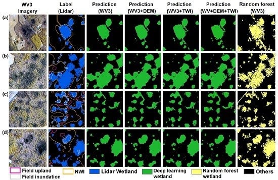
To evaluate the accuracy of deep learning inundation maps at the object level, we compared our deep learning inundation maps against lidar intensity-derived inundation labels in 64 image patches that overlapped with field polygons and were not used in model training. Meanwhile, the wetland inundation maps produced by Vanderhoof et al. [12] were also split to the 256*256 pixel size using the moving window approach in this study to coordinate with our validation analysis.

We first quantified the relationships between the wetland inundation area estimated from different results and the lidar intensity-derived inundation labels in the 64 validation image patches. In our study, the wetland inundation area was calculated by counting the total number of inundated pixels in each image patch. We employed the r-squared (R²) and root-mean-square error (RMSE) for the quantitative comparison of the relationships.

Moreover, to further quantify the overlap ratio of wetland inundation objects predicted in different results against the lidar intensity-derived inundation labels, we adopted a metric based on the intersection over union (IoU), also known as the Jaccard index, which measures the overlap between two objects by dividing the area intersected by the area of union (Equation (6)) [39]. The value of IoU ranges from 0 to 1. If measured IoU is 0.5 or above, it is usually considered as a true positive, otherwise, it is considered as a false positive.

$$IoU\left(A, B\right)=\frac{Area\left(A{{\displaystyle \cap }}^{\text{}}B\right)}{Area\left(A{{\displaystyle \cup }}^{\text{}}B\right)}$$

(7)

where A and B correspond to wetland inundation objects predicted in different results and lidar intensity-derived inundation labels, respectively, in this study.

3. Results

3.1. Classification Accuracy at the Pixel Level

The spatial distribution of forested wetland inundation over the entire upper Choptank River watershed was predicted by deep learning algorithms based on the U-Net network using 2015 WV3 imagery and different combinations of topographic information (i.e., DEM, TWI and DEM + TWI). Figure 6 shows the deep learning inundation map at the watershed scale using WV3 and TWI as model inputs. In our study, we used the false-color-composited WV3 imagery with the Near-IR2, Red Edge and Yellow bands, respectively, in red, green and blue channels for a better visual display of wetland inundation, because the combination of these three bands contains a larger amount of information than other combinations [40].

Based on the confusion matrix sampled from field polygons, our predictions derived from deep learning networks showed a consistently higher OA than the random forest output (

Table 2. Accuracy assessments using field data. The variables in the parentheses are the data input used for our deep learning network or the random forest model. WV3: WorldVview-3, DEM: Digital Elevation Model, TWI: Topographic Wetness Index.

	Prediction (WV3)	Prediction (WV3 + DEM)	Prediction (WV3 + TWI)	Prediction (WV3 + DEM + TWI)	Random Forest (WV3)
Overall Accuracy (%)	92	95	95	95	91
Precision (%)	99	100	99	99	98
Recall (%)	84	90	91	89	83
F1 score	0.91	0.95	0.95	0.94	0.90
Kappa	0.84	0.90	0.90	0.89	0.81

). Specifically, the OA of our prediction using WV3 dataset was 92% with F1 score = 0.91 and Kappa = 0.84. The OA of the random forest output, which was also based on WV3, was 91% with F1 score = 0.90 and Kappa = 0.81. By including either topographic data (i.e., DEM or TWI) into the deep learning model, our OA increased to 95% with a higher F1 score (>= 0.94) and Kappa coefficient (>= 0.89) (Table 2). In our study, the lidar intensity-derived inundation labels also showed a high overall accuracy (95%) compared to the 2015 field polygons, which was validated by a separate group of field points. The precision and recall of lidar intensity-derived inundation labels were 100% and 90%, respectively.

3.2. Classification Accuracy at the Object Level

We further compared our deep learning inundation maps with the random forest output, as well as the NWI wetland dataset at the object level using the lidar intensity-derived inundation labels (i.e., 64 validation image patches) as a reference. Generally, our deep learning inundation maps showed a much clearer pattern of wetland inundation than the random forest output (Figure 7). Each wetland was captured as well as an individual object. By contrast, the random forest output created a distinct “salt-and-pepper” appearance in the classification, and was easily mixed with ditches and roads (Figure 7). Additionally, the NWI wetland maps showed a much broader extent than both our predictions and the random forest inundation output (Figure 7).

The WorldView-3 (WV3) imagery in the first column was shown in false color (Red channel: Near-IR2, Green channel: Red Edge, Blue channel: Yellow). DEM: Digital Elevation Model, TWI: Topographic Wetness Index, NWI: National Wetlands Inventory

The estimates of wetland inundation areas in our predictions were very close to the 1:1 line against the estimates of lidar intensity-derived inundation areas with R² ≥ 0.96 and RMSE ≤ 0.59 (p < 0.001) (Figure 8). The inclusion of the DEM or TWI data in the deep learning model slightly improved the relationship with a higher R² and lower RMSE (Figure 8). In comparison, the R² and RMSE between the random forest inundation areas and lidar intensity-derived inundation areas were 0.85 and 1.25, respectively.

There was a high degree of overlap between wetland inundation in our predictions and the lidar intensity-derived inundation labels. The median IoU between our predictions using WV3 and the lidar inundation labels was 66%, while the median IoU between the random forest output and the lidar inundation labels was 51% (Figure 9). By integrating the TWI into the deep learning model, our median IoU increased to 70% (Figure 9).

4. Discussion

Foundational mapping and timely updates of forested wetland inundation using high-resolution remote sensing data are essential and remain a challenge due in part to the complexity of wetland features that are subject to temporal change due to natural and anthropogenic influences. In our study, we built a state-of-the-art deep learning network based on U-Net architecture to classify wetland inundation within the upper Choptank River watershed using WorldView 3 imagery and topographic datasets (i.e., DEM and TWI). Our deep learning network represents a novel fully convolutional network for semantic segmentation, which integrates both the spatial and spectral information of input images, and hence is fundamentally different than traditional classification approaches, e.g., random forest, without considering spatial context feature. To train our deep learning network, we used a lidar intensity image to derive wetland inundation labels. Our results showed a higher classification accuracy than the pixel-based random forest output at both the pixel and object level. The overall accuracy was increased slightly by adding topographic information into the deep learning network. The effectiveness of using lidar intensity to derive wetland inundation labels for model training and the efficiency of the deep learning network to classify forested wetland inundation during the leaf-off season are the primary strengths of this study.

Creating the label data for deep learning models using high-resolution data sources has proven challenging due to the scarcity of high-resolution references, as well as the complex information provided by the images. By contrast, traditional machine learning approaches are easier to train using a small number of training data points [7,12]. However, this study benefited from the effectiveness of highly accurate inundation labels using lidar intensity. Wetland inundation labels derived from the 2007 lidar intensity matched quite well with inundation extent, as shown in the 2015 WV3 imagery (Figure 3), and had an overall accuracy of 95% compared to the 2015 field polygons. Given that the topography remained constant, this indicated a similar climate condition between these two years. However, compared to the DEM data, lidar intensity data are often less available. In our study, lidar intensity data collected for model training only covered ~4% of the watershed extent, and was located in a region dominated by large numbers of geographically isolated wetlands with fewer floodplain wetlands (Figure 3). Thus, the classification accuracy of the inundation extent along the floodplains was difficult to evaluate.

Furthermore, the applicability of our deep learning model to locations far away from the training area was not evaluated in our study, as previous studies suggested that model degradation might occur in both traditional approaches or sematic deep learning networks in new geographic locations [41]. Thus, examining the availability and implications of lidar intensity would be valuable for future wetland inundation mapping. In addition, our method only applies to leaf-off wetlands identification using lidar intensity-derived inundation labels and high-resolution optical imagery, as the remote sensing imagery collected in the growing season mostly captures the structure of leaf-on tree canopy.

Our classification accuracy showed a slight increase by the inclusion of topographic datasets in our deep learning model (Figure 8 and Figure 9), which also supports previous studies showing that topographic information could contribute to land cover classification [42]. However, since our study area was in a low relief setting, wetland inundation classification was still primarily driven by the WV3 data, which documented the critical spectral and spatial contexture properties of water extent below forest canopy (Table 2, Figure 7, Figure 8 and Figure 9). Only a small improvement in classification accuracy was gained by using either the DEM or TWI. However, we found that the inundation extent along the floodplains using DEM was slightly larger than that using the TWI (results not shown), which needs further investigation due to the limited training for floodplain wetlands in this study.

Our results showed a higher accuracy using deep learning models than the traditional random forest output at both the pixel level and object level (Table 2, Figure 7, Figure 8 and Figure 9). Our deep learning approach to classify image pixels with inundation labels is object-oriented, which extracts characteristic features from wetland objects that exist in input images and assigns a probability of inundation to each pixel. In contrast, in random forest, the probability of each class per pixel is based on the spectral features inherent in the image. In high-resolution remote sensing data, pixel-based spectral features contain less information than object-based spatial features. For example, inundation under the forest canopy is not only characterized by its spectral features (color of the water or tree canopy), but also by how these elements are arranged in an image. However, we should note that the 2-m random forest output obtained in this study was only derived from WV3 datasets. Vanderhoof et al. [12] also maximized the accuracy of the inundation map by adding RADARSAT-2 data within a random forest model, and in this way increased overall accuracy to 94%. However, the spatial resolution of the derived map was decreased to 5.6 m due to the coarser resolution of RADARSAT-2.

Comparison of our deep learning inundation maps to the NWI geospatial dataset supports assessment of deep learning techniques for future integration within operational wetland mapping. Although this study produced maps of inundation, and not wetlands, it should be noted that a large portion of wetlands at the study site would be inundated at this time of year. Furthermore, the NWI dataset includes information on wetland hydroperiod (i.e., water regime), and the deep learning approach developed as part of this study could be used to refine these water regime codes in the future, especially if inundation maps can be produced during different times of the year and/or under multiple weather conditions. The NWI dataset, which was derived primarily through the manual interpretation of fine spatial resolution optical images (e.g., NAIP), showed a broader wetland extent in comparison with our deep learning inundation maps and the random forest inundation output (Figure 7, Figure 8 and Figure 9), even though our predictions were based on WV3 that were collected at a time of year when the expression of inundation within wetlands is maximized. It is likely that this difference was caused by two primary drivers: 1) the presence of saturated wetlands which do not exhibit inundation, and 2) the NWI dataset’s larger targeted mapping unit (i.e., ~0.20 ha). It is also possible that some of this disagreement could be caused by substantial errors of omission existing in forested wetlands in NWI maps and wetland drainage between 2007–2013 (NAIP acquisition date) and 2015 (WV3 acquisition date) [11]. This study demonstrates that deep learning techniques can improve the quality of inundation maps. Addressing the ability of deep learning to map a wider range of wetlands, including those with a saturated water regime, and the ability of deep learning techniques to support mapping over larger areas would greatly enhance the utility of these techniques for supporting operational wetland mapping, especially at regional and national scales.

5. Conclusions

Mapping forested wetland inundation is an important first step of understanding the responses of wetlands to weather variability and climate change. In this study, we demonstrated a novel framework based on the U-Net architecture to identify forested wetland inundation in the Delmarva Peninsula, United States. We produced the maps of forested wetland inundation in 2015 using WV3 imagery and topographic information. Small to large forested wetland inundation was successfully captured with an overall accuracy of 95%. Wetland inundation patterns classified by the deep learning network showed higher consistency with lidar intensity-derived inundation labels. Our study demonstrated the effectiveness of deep learning models for mapping forested wetland inundation at the object level with high accuracy and less “salt-and-pepper” effects, using high-resolution remote sensing imagery and lidar intensity data.

References

1. Tiner, R.W. Geographically isolated wetlands of the United States. Wetlands 2003, 23, 494–516. [Google Scholar] [CrossRef]
2. Cohen, M.J.; Creed, I.F.; Alexander, L.; Basu, N.B.; Calhoun, A.J.; Craft, C.; D’Amico, E.; DeKeyser, E.; Fowler, L.; Golden, H.E.; et al. Do geographically isolated wetlands influence landscape functions? Proc. Natl. Acad. Sci. USA 2016, 113, 1978–1986. [Google Scholar] [CrossRef] [PubMed] [Green Version]
3. Lang, M.W.; Kasischke, E.S. Using C-Band Synthetic Aperture Radar Data to Monitor Forested Wetland Hydrology in Maryland’s Coastal Plain, USA. IEEE Trans. Geosci. Remote Sens. 2008, 46, 535–546. [Google Scholar] [CrossRef]
4. Stedman, S.; Dahl, T.E. Status and Trends of Wetlands in the Coastal Watersheds of the Eastern United States 1998 to 2004. Available online: https://www.fws.gov/wetlands/Documents/Status-and-Trends-of-Wetlands-in-the-Coastal-Watersheds-of-the-Eastern-United-States-1998-to-2004.pdf (accessed on 14 February 2020).
5. DeVries, B.; Huang, C.; Lang, M.; Jones, J.; Huang, W.; Creed, I.; Carroll, M. Automated Quantification of Surface Water Inundation in Wetlands Using Optical Satellite Imagery. Remote Sens. 2017, 9, 807. [Google Scholar] [CrossRef] [Green Version]
6. Huang, C.; Peng, Y.; Lang, M.; Yeo, I.-Y.; McCarty, G. Wetland inundation mapping and change monitoring using Landsat and airborne LiDAR data. Remote Sens. Environ. 2014, 141, 231–242. [Google Scholar] [CrossRef]
7. Jin, H.; Huang, C.; Lang, M.W.; Yeo, I.-Y.; Stehman, S.V. Monitoring of wetland inundation dynamics in the Delmarva Peninsula using Landsat time-series imagery from 1985 to 2011. Remote Sens. Environ. 2017, 190, 26–41. [Google Scholar] [CrossRef] [Green Version]
8. Zou, Z.; Xiao, X.; Dong, J.; Qin, Y.; Doughty, R.B.; Menarguez, M.A.; Zhang, G.; Wang, J. Divergent trends of open-surface water body area in the contiguous United States from 1984 to 2016. Proc. Natl. Acad. Sci. USA 2018, 115, 3810–3815. [Google Scholar] [CrossRef] [Green Version]
9. Huang, W.; DeVries, B.; Huang, C.; Lang, M.; Jones, J.; Creed, I.; Carroll, M. Automated Extraction of Surface Water Extent from Sentinel-1 Data. Remote Sens. 2018, 10, 797. [Google Scholar] [CrossRef] [Green Version]
10. Bolanos, S.; Stiff, D.; Brisco, B.; Pietroniro, A. Operational Surface Water Detection and Monitoring Using Radarsat 2. Remote Sens. 2016, 8, 285. [Google Scholar] [CrossRef] [Green Version]
11. Lang, M.W.; McCarty, G.W. Lidar Intensity for Improved Detection of Inundation Below the Forest Canopy. Wetlands 2009, 29, 1166–1178. [Google Scholar] [CrossRef]
12. Vanderhoof, M.K.; Distler, H.E.; Mendiola, D.T.G.; Lang, M. Integrating Radarsat-2, Lidar, and Worldview-3 Imagery to Maximize Detection of Forested Inundation Extent in the Delmarva Peninsula, USA. Remote Sens. 2017, 9, 105. [Google Scholar] [CrossRef] [Green Version]
13. Wu, Q.; Lane, C.R.; Li, X.; Zhao, K.; Zhou, Y.; Clinton, N.; DeVries, B.; Golden, H.E.; Lang, M.W. Integrating LiDAR data and multi-temporal aerial imagery to map wetland inundation dynamics using Google Earth Engine. Remote Sens. Environ. 2019, 228, 1–13. [Google Scholar] [CrossRef] [Green Version]
14. Lang, M.; McCarty, G.; Oesterling, R.; Yeo, I.-Y. Topographic Metrics for Improved Mapping of Forested Wetlands. Wetlands 2012, 33, 141–155. [Google Scholar] [CrossRef]
15. Chan, R.H.; Chung-Wa, H.; Nikolova, M. Salt-and-pepper noise removal by median-type noise detectors and detail-preserving regularization. IEEE Trans. Image Process. 2005, 14, 1479–1485. [Google Scholar] [CrossRef] [PubMed]
16. Khatami, R.; Mountrakis, G.; Stehman, S.V. A meta-analysis of remote sensing research on supervised pixel-based land-cover image classification processes: General guidelines for practitioners and future research. Remote Sens. Environ. 2016, 177, 89–100. [Google Scholar] [CrossRef] [Green Version]
17. Ding, P.; Zhang, Y.; Deng, W.-J.; Jia, P.; Kuijper, A. A light and faster regional convolutional neural network for object detection in optical remote sensing images. ISPRS J. Photogramme. Remote Sens. 2018, 141, 208–218. [Google Scholar] [CrossRef]
18. Kellenberger, B.; Marcos, D.; Tuia, D. Detecting mammals in UAV images: Best practices to address a substantially imbalanced dataset with deep learning. Remote Sens. Environ. 2018, 216, 139–153. [Google Scholar] [CrossRef] [Green Version]
19. Zhao, H.; Shi, J.; Qi, X.; Wang, X.; Jia, J. Pyramid Scene Parsing Network. In Proceedings of the 2017 IEEE Conference on Computer Vision and Pattern Recognition (CVPR), Honolulu, HI, USA, 21–26 July 2017; pp. 6230–6239. [Google Scholar]
20. Badrinarayanan, V.; Kendall, A.; Cipolla, R. SegNet: A Deep Convolutional Encoder-Decoder Architecture for Image Segmentation. IEEE Trans. Pattern Anal. Mach. Intell. 2017, 39, 2481–2495. [Google Scholar] [CrossRef]
21. Ronneberger, O.; Fischer, P.; Brox, T. U-Net: Convolutional Networks for Biomedical Image Segmentation; Springer International Publishing: Cham, Switzerland, 2015; pp. 234–241. [Google Scholar]
22. Chen, L.C.; Papandreou, G.; Kokkinos, I.; Murphy, K.; Yuille, A.L. DeepLab: Semantic Image Segmentation with Deep Convolutional Nets, Atrous Convolution, and Fully Connected CRFs. IEEE Trans. Pattern Anal. Mach. Intell. 2018, 40, 834–848. [Google Scholar] [CrossRef]
23. Du, Z.; Yang, J.; Ou, C.; Zhang, T. Smallholder Crop Area Mapped with a Semantic Segmentation Deep Learning Method. Remote Sens. 2019, 11, 888. [Google Scholar] [CrossRef] [Green Version]
24. Zhang, X.; Han, L.; Dong, Y.; Shi, Y.; Huang, W.; Han, L.; González-Moreno, P.; Ma, H.; Ye, H.; Sobeih, T. A Deep Learning-Based Approach for Automated Yellow Rust Disease Detection from High-Resolution Hyperspectral UAV Images. Remote Sens. 2019, 11, 1554. [Google Scholar] [CrossRef] [Green Version]
25. Sun, Y.; Huang, J.; Ao, Z.; Lao, D.; Xin, Q. Deep Learning Approaches for the Mapping of Tree Species Diversity in a Tropical Wetland Using Airborne LiDAR and High-Spatial-Resolution Remote Sensing Images. Forests 2019, 10, 1047. [Google Scholar] [CrossRef] [Green Version]
26. Flood, N.; Watson, F.; Collett, L. Using a U-net convolutional neural network to map woody vegetation extent from high resolution satellite imagery across Queensland, Australia. Int. J. Appl. Earth Obs. Geoinf. 2019, 82. [Google Scholar] [CrossRef]
27. Li, R.; Liu, W.; Yang, L.; Sun, S.; Hu, W.; Zhang, F.; Li, W. DeepUNet: A Deep Fully Convolutional Network for Pixel-Level Sea-Land Segmentation. IEEE J. Sel. Topics Appl. Earth Obs. Remote Sens. 2018, 11, 3954–3962. [Google Scholar] [CrossRef] [Green Version]
28. Lowrance, R.; Altier, L.S.; Newbold, J.D.; Schnabel, R.R.; Groffman, P.M.; Denver, J.M.; Correll, D.L.; Gilliam, J.W.; Robinson, J.L.; Brinsfield, R.B.; et al. Water Quality Functions of Riparian Forest Buffers in Chesapeake Bay Watersheds. Environ. Manage 1997, 21, 687–712. [Google Scholar] [CrossRef]
29. Shedlock, R.J.; Denver, J.M.; Hayes, M.A.; Hamilton, P.A.; Koterba, M.T.; Bachman, L.J.; Phillips, P.J.; Banks, W.S. Water-quality assessment of the Delmarva Peninsula, Delaware, Maryland, and Virginia; Rresults of Investigations, 1987-91; 2355A; USGS: Reston, VA, USA, 1999. [Google Scholar]
30. Ator, S.W.; Denver, J.M.; Krantz, D.E.; Newell, W.L.; Martucci, S.K. A Surficial Hydrogeologic Framework for the Mid-Atlantic Coastal Plain; 1680; USGS: Reston, VA, USA, 2005. [Google Scholar]
31. Homer, C.; Dewitz, J.; Yang, L.M.; Jin, S.; Danielson, P.; Xian, G.; Coulston, J.; Herold, N.; Wickham, J.; Megown, K. Completion of the 2011 National Land Cover Database for the Conterminous United States - Representing a Decade of Land Cover Change Information. Photogramm. Eng. Rem. S 2015, 81, 345–354. [Google Scholar] [CrossRef]
32. Vanderhoof, M.K.; Distler, H.E.; Lang, M.W.; Alexander, L.C. The influence of data characteristics on detecting wetland/stream surface-water connections in the Delmarva Peninsula, Maryland and Delaware. Wetlands Ecol. Manage. 2017, 26, 63–86. [Google Scholar] [CrossRef]
33. Lang, M.; McDonough, O.; McCarty, G.; Oesterling, R.; Wilen, B. Enhanced Detection of Wetland-Stream Connectivity Using LiDAR. Wetlands 2012, 32, 461–473. [Google Scholar] [CrossRef]
34. Li, X.; McCarty, G.W.; Lang, M.; Ducey, T.; Hunt, P.; Miller, J. Topographic and physicochemical controls on soil denitrification in prior converted croplands located on the Delmarva Peninsula, USA. Geoderma 2018, 309, 41–49. [Google Scholar] [CrossRef]
35. Li, X.; McCarty, G.W.; Karlen, D.L.; Cambardella, C.A.; Effland, W. Soil Organic Carbon and Isotope Composition Response to Topography and Erosion in Iowa. J. Geophys. Res. Biogeosci. 2018, 123, 3649–3667. [Google Scholar] [CrossRef] [Green Version]
36. Lang, M.W.; Kim, V.; McCarty, G.W.; Li, X.; Yeo, I.Y.; Huang, C. Improved Detection of Inundation under Forest Canopy Using Normalized LiDAR Intensity Data. Remote Sens. 2020, 12, 707. [Google Scholar] [CrossRef] [Green Version]
37. Diakogiannis, F.I.; Waldner, F.; Caccetta, p.; Wu, C. ResUNet-a: A deep learning framework for semantic segmentation of remotely sensed data. arXiv 2019, arXiv:1904.00592. [Google Scholar]
38. Zhu, W.; Huang, Y.; Zeng, L.; Chen, X.; Liu, Y.; Qian, Z.; Du, N.; Fan, W.; Xie, X. AnatomyNet: Deep learning for fast and fully automated whole-volume segmentation of head and neck anatomy. Med. Phys. 2019, 46, 576–589. [Google Scholar] [CrossRef] [PubMed] [Green Version]
39. Choi, S.-S.; Cha, S.-H.; Tappert, C.C. A survey of binary similarity and distance measures. J. Syst. Cyberne. Inform. 2010, 8, 43–48. [Google Scholar]
40. Li, J.; Chen, J.; Sun, Y. Research of Color Composite of WorldView-2 Based on Optimum Band Combination. Int. J. Adv. Informa. Sci. Service Sci. 2013, 5, 791–798. [Google Scholar] [CrossRef]
41. Hayes, M.M.; Miller, S.N.; Murphy, M.A. High-resolution landcover classification using Random Forest. Remote Sens. Lett. 2014, 5, 112–121. [Google Scholar] [CrossRef]
42. Benediktsson, J.A.; Swain, P.H.; Ersoy, O.K. Neural Network Approaches Versus Statistical-Methods in Classification of Multisource Remote-Sensing Data. IEEE Trans. Geosci. Remote Sens. 1990, 28, 540–552. [Google Scholar] [CrossRef]
Figure 1. Map of study area in the upper Choptank River watershed located in the Delmarva Peninsula, USA. (a) The 2-m WorldView3 (WV3) imagery (acquisition date: April 6, 2015) in a natural color composite. (b) The 2-m light detection and ranging (lidar) digital elevation model (DEM) generated from three separate lidar collections. (c) Topographic wetness index (TWI) derived from the 2-m lidar DEM, which was generated from the System for Automated Geoscientific Analysis (SAGA) v. 7.3.0.
Remotesensing 12 00644 g001
Figure 2. Workflow of wetland inundation mapping in this study. DEM: Digital Elevation Model, TWI: Topographic Wetness Index, NWI: National Wetland Inventory.
Remotesensing 12 00644 g002
Figure 3. Wetland inundation labels derived from the lidar intensity for model training and validation. (a) A subset of WorldView-3 (WV3) imagery shown in a false color composite (Red channel: Near-IR2, Green channel: Red Edge, Blue channel: Yellow). (b) Wetland inundation labels binarized from a normalized lidar intensity image, which was shown in a vector format and processed in ArcGIS 10.6 using the raster to polygon tool.
Remotesensing 12 00644 g003
Figure 4. Schematic of the architecture used in our study. The numbers below the first and last bars showed the layers of images in model input and output, respectively. The numbers below the other bars showed the number of convolutional neural network (CNN) layers.
Remotesensing 12 00644 g004
Figure 5. An example of image patches split using an overlapped moving window. We randomly chose two image patches (a,b) from the training dataset. RGB: Red, Green, Blue, IR: infrared, DEM: Digital Elevation Model, TWI: Topographic Wetness Index.
Remotesensing 12 00644 g005
Figure 6. Forested wetland inundation map classified using WorldView-3 (WV3) + topographic wetness index (TWI) using deep learning method. (a,b) are zoom-in WV3 imagery and deep learning inundation map, respectively in depressional wetlands in box 1. (c,d) are zoom-in WV3 imagery and deep learning inundation map, respectively in floodplains in box 2. WV3 imageries in (a) and (c) are shown in false color (Red channel: Near-IR2, Green channel: Red Edge, and Blue channel: Yellow).
Remotesensing 12 00644 g006
Figure 7. Comparison of forested wetland inundation predicted in our study with the lidar intensity-derived inundation labels, the random forest output, and the NWI geospatial dataset, which depicts wetlands. The variables in the parentheses are the data input used for our deep learning network or the random forest model. We randomly chose four image patches (a-d) out of 64 validation image patches as examples.
Remotesensing 12 00644 g007
Figure 8. Comparisons of wetland areas predicted by deep learning algorithms (ad) in our study and random forest (e) against the lidar intensity-derived inundation labels. Each black point represents the estimate of wetland area in each image out of the 64 image patches. The black dashed line is the 1:1 line. The blue line is the linear regression model. The blue shadow shows the 95% confidence interval of the linear regression model. WV3: WorldView-3, DEM: Digital Elevation Model, TWI: Topographic Wetness Index, RMSE: Root Mean Square Error.
Remotesensing 12 00644 g008
Figure 9. The intersection of union (IoU) calculated between different wetland inundation results and the lidar intensity-derived inundation labels. The percentages above each boxplot bar are the median IoU values. WV3: WorldView-3, DEM: Digital Elevation Model, TWI: Topographic Wetness Index.
Remotesensing 12 00644 g009