Precise and Robust Ship Detection for High-Resolution SAR Imagery Based on HR-SDNet

Abstract

Ship detection in high-resolution synthetic aperture radar (SAR) imagery is a challenging problem in the case of complex environments, especially inshore and offshore scenes. Nowadays, the existing methods of SAR ship detection mainly use low-resolution representations obtained by classification networks or recover high-resolution representations from low-resolution representations in SAR images. As the representation learning is characterized by low resolution and the huge loss of resolution makes it difficult to obtain accurate prediction results in spatial accuracy; therefore, these networks are not suitable to ship detection of region-level. In this paper, a novel ship detection method based on a high-resolution ship detection network (HR-SDNet) for high-resolution SAR imagery is proposed. The HR-SDNet adopts a novel high-resolution feature pyramid network (HRFPN) to take full advantage of the feature maps of high-resolution and low-resolution convolutions for SAR image ship detection. In this scheme, the HRFPN connects high-to-low resolution subnetworks in parallel and can maintain high resolution. Next, the Soft Non-Maximum Suppression (Soft-NMS) is used to improve the performance of the NMS, thereby improving the detection performance of the dense ships. Then, we introduce the Microsoft Common Objects in Context (COCO) evaluation metrics, which provides not only the higher quality evaluation metrics average precision (AP) for more accurate bounding box regression, but also the evaluation metrics for small, medium and large targets, so as to precisely evaluate the detection performance of our method. Finally, the experimental results on the SAR ship detection dataset (SSDD) and TerraSAR-X high-resolution images reveal that (1) our approach based on the HRFPN has superior detection performance for both inshore and offshore scenes of the high-resolution SAR imagery, which achieves nearly 4.3% performance gains compared to feature pyramid network (FPN) in inshore scenes, thus proving its effectiveness; (2) compared with the existing algorithms, our approach is more accurate and robust for ship detection of high-resolution SAR imagery, especially inshore and offshore scenes; (3) with the Soft-NMS algorithm, our network performs better, which achieves nearly 1% performance gains in terms of AP; (4) the COCO evaluation metrics are effective for SAR image ship detection; (5) the displayed thresholds within a certain range have a significant impact on the robustness of ship detectors.

1. Introduction

The high-resolution synthetic aperture radar (SAR) images are provided by the airborne and spaceborne SAR sensor with the capability of working in all-weather and all-day. Nowadays, these SAR images have been diffusely applied in multiple fields, such as environmental management, land and resources administration, natural disaster forewarn, and national defense [1,2]. In particular, such fields as maritime transport safety and fishery enforcement [3,4,5] tend to make use of the high-resolution SAR images to ship detection, which is the main topic in this paper.

Ship detection in SAR imagery is a complicated problem, mainly containing two tasks to be solved. One is the recognition problem, where the detectors separate the ships from the backgrounds and set accurate ship class labels. Another is the location problem, assigning precise bounding boxes for different ships. However, due to the complex background, the ships are difficult to detect accurately, and the small ships are easy to be ignored, and the dense ships are difficult to distinguish, as shown in Figure 1. Therefore, this paper focuses on an accurate and robust ship detection method for both inshore and offshore scenes of high-resolution SAR imagery.

Traditional ship detection approaches are mainly constant false alarm rates (CFAR) based on the statistical distributions of the sea clutter [6,7,8] and the extracted features are based on the machine learning method [9,10,11,12]. However, these conventional methods are highly dependent on the distributions of features predefined by humans [9,13,14,15], degrading the performance of ship detection for new SAR imagery [9,15]. Therefore, these methods are difficult to perform ship detection accurately and robustly. In addition, many ship detection methods based on superpixels have been proposed. Li et al. [16] came up with an improved superpixel-level constant false alarm rate (CFAR) detection method. He et al. [17] proposed a method for automatically detecting ships using three superpixel-level dissimilarity measures. Lin et al. [18] proposed a superpixel-level Fisher vector to describe the difference between the target and clutter. However, it is also difficult for these methods to accurately detect ships for both inshore and offshore scenes.

In recent years, the deep learning theory has been growing fast, leading to emerging breakthroughs in object detection conducted by the researchers from the computer vision field. At present, deep learning is viewed as the future tendency and plays an important role in object detection, and the emerging algorithms can be roughly classified into two categories: (1) two-stage detection algorithm, first generating region proposals that filter most of the negative samples, then performing the candidate region classification (generally need to be refined for location). Typical examples of such algorithms are region convolutional neural networks (R-CNN) algorithms based on region proposals, such as regions with CNN features (R-CNN) [19], Fast R-CNN [20], Faster R-CNN [21], Feature Pyramid Networks (FPN) [22], Mask R-CNN [23], Cascade R-CNN [24], etc.; (2) one-stage detection algorithm, getting rid of the region proposal stage, directly detect the object by obtaining its coordinate values and the class probability. The typical one-stage algorithms are You Only Look Once (YOLO v1-v3) [25,26,27], Single Shot MultiBox Detector (SSD) [28], Deconvolutional Single Shot Detector (DSSD) [29], Feature Fusion Single Shot Multibox Detector (FSSD) [30], RetinaNet [31], etc. In short, the two-stage algorithms have higher accuracy than the one-stage, but the one-stage is faster and more simple to train.

Nowadays, researchers have already introduced the deep learning method for ship detection in the SAR imagery field. Liu et al. [32] applied spectral residual based on land-sea segmentation to realize automatic selecting the candidate ship location and convolutional neural networks to ship discrimination. Kang et al. [33] designed a contextual region-based R-CNN with multilayer fusion to improve the performance of detecting the small ships. Kang et al. [34] proposed a modified faster R-CNN method with CFAR to provide a solution to the multi-scale problem in small ship detection. Li et al. [35] introduced the faster R-CNN method into the ship detection field with the additional four strategies, such as feature fusion, while building up a ship-related dataset suitable for testifying the new detection method. Wang et al. [36] used a single shot multi-box detector to acquire high-detection accuracy as well as the relatively high speed and added transfer learning to the process to reduce the false positives. Chang et al. [37] adopted YOLOv2 to detect ships in SAR images and reduced the computational expenses. Wang et al. [3] aimed at the multi-scale problem and alleviated the dependence of the statistical models or extracted features, exploiting a RetinaNet to obtain high ship detection accuracy. Zhang et al. [38] proposed a Grid Convolutional Neural Network to solve real-time detection problems. Cui et al. [1] came up with a dense attention pyramid network for multi-scale ship detection in high-resolution SAR images.

However, the existing methods of SAR ship detection mainly use low-resolution representations obtained by classification networks or recover high-resolution representations from low-resolution representations for ship detection in SAR images. Therefore, these networks are not suitable for ship detection at the region-level because the representation learning is characterized by low resolution and the huge loss of resolution makes it difficult to obtain accurate prediction results in spatial accuracy. Especially inshore and offshore scenes, the results are even worse. In this paper, a novel ship detection method based on a high-resolution ship detection network (HR-SDNet) for high-resolution SAR imagery is proposed.

First, a novel high-resolution feature pyramid network (HRFPN) is proposed to take full advantage of the feature maps of high-resolution and low-resolution convolutions for SAR image ship detection. The HRFPN connects high-to-low resolution subnetworks in parallel and can maintain the high resolution.

Next, a region proposal network (RPN) [21,22] is used to generate candidate ship bounding box proposals. Moreover, a cascade structure demonstrates its effectiveness on various tasks such as object detection [24,39,40]. We will use a cascading structure to the SAR image ship detection network for bounding boxes regression and classification to improve the quality of ship detection. Furthermore, Soft Non-Maximum Suppression (Soft-NMS) [41] is used to improve the performance of the NMS. It uses the linear penalty function to reduce the detection scores of all other neighbors, thereby improving the detection performance of the dense ships.

Then, we introduce Microsoft Common Objects in Context (COCO) [42] evaluation metrics to precisely evaluate the detection performance of our method. It includes not only the higher quality evaluation metrics average precision (AP) for more accurate bounding box regression, but also the evaluation metrics for small, medium, and large targets. Moreover, we analyze the effect of image preprocessing on the robust performance of our detector by the clipping function of the displayed image [43].

Finally, it is quite easy to exploit the HR-SDNet, and it can be used for end-to-end training. Our results demonstrate that the proposed framework gains much better performance than the existing state-of-the-art single-model ship detectors on the SSDD dataset [35], especially using the higher quality evaluation metrics. Furthermore, the experiments on the TerraSAR-X [44] high-resolution images from the strait of Singapore and Gibraltar prove that our method is effective and robust. In summary, these results validate the effectiveness and robustness of our proposed method in the high-resolution SAR imagery.

A summary of the main contributions of our work are as follows:

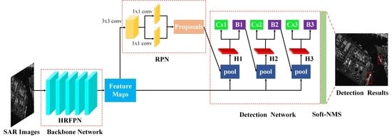
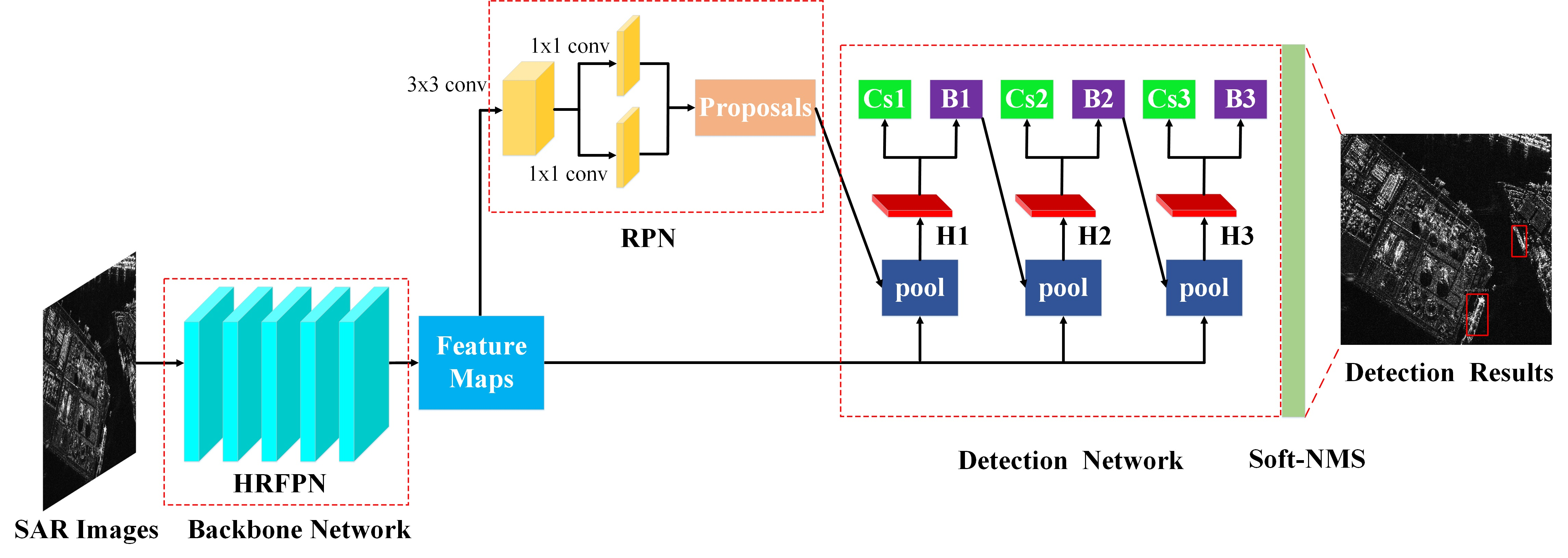
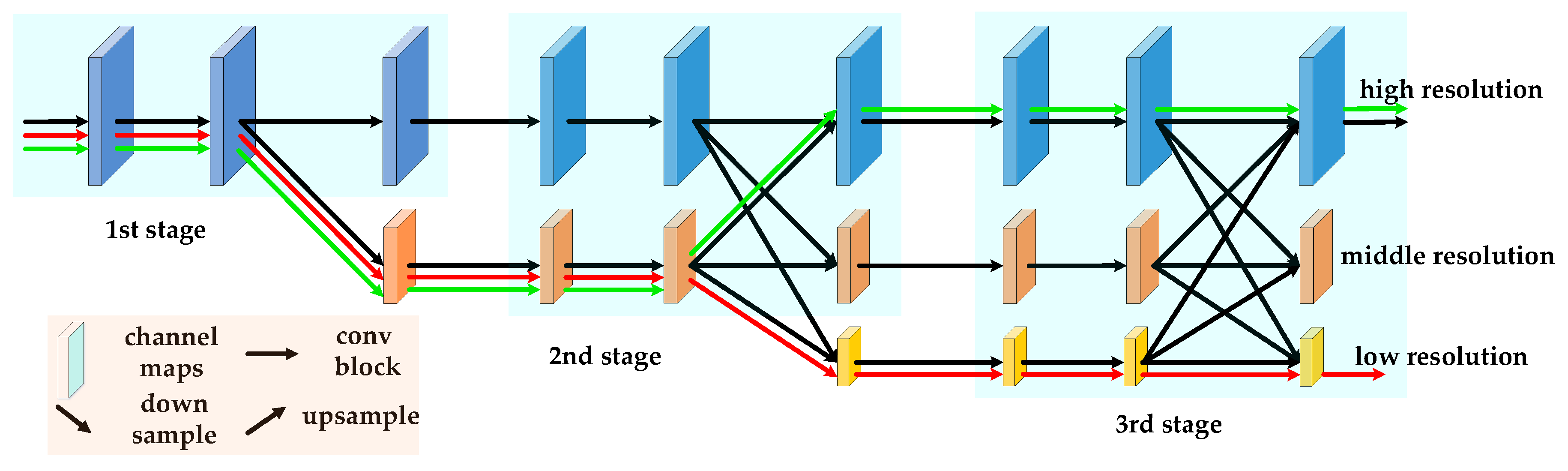
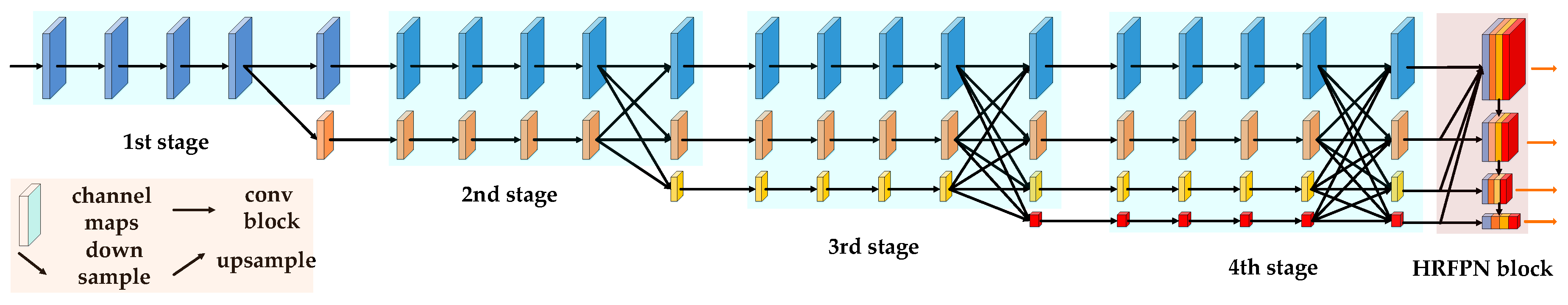
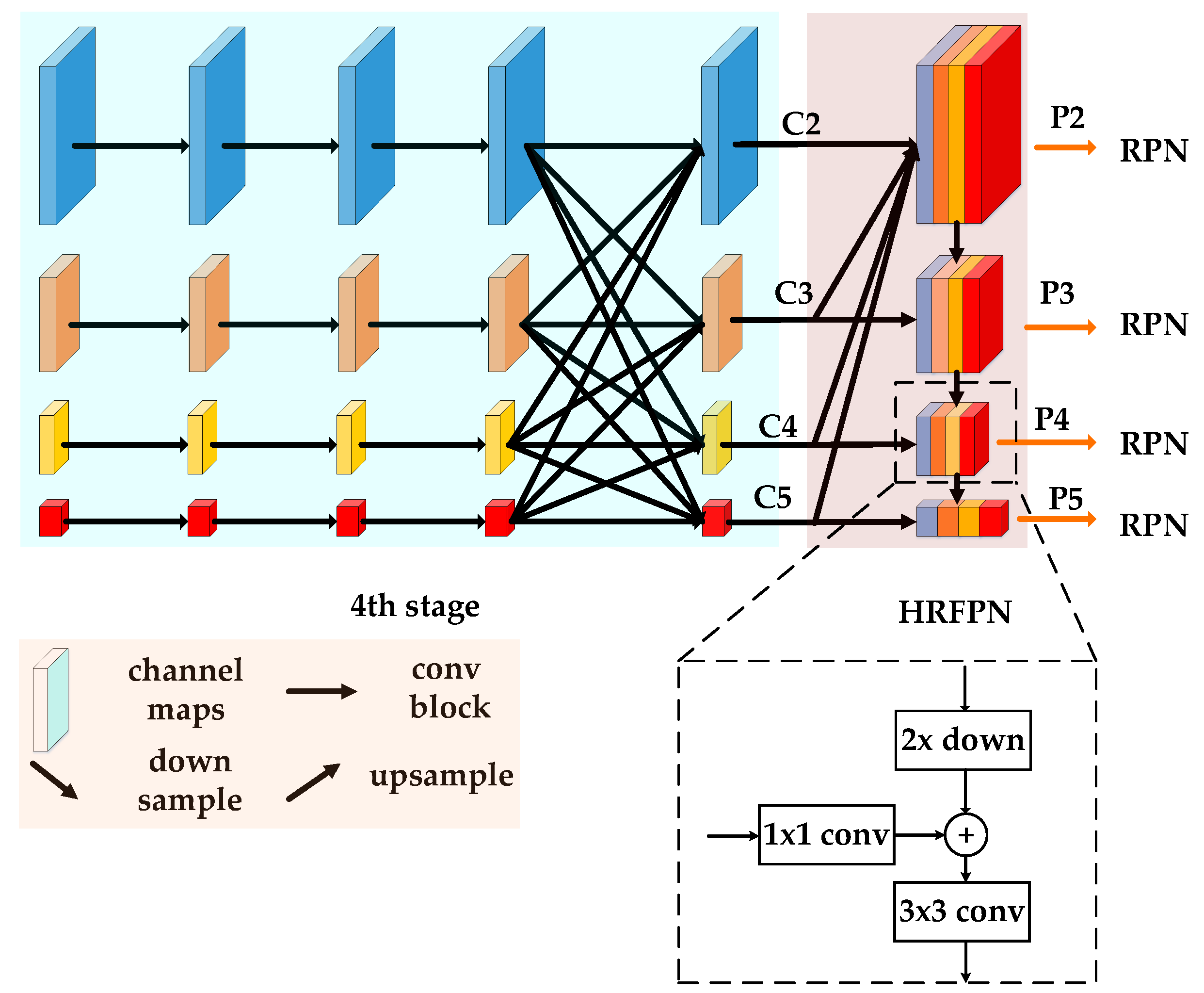
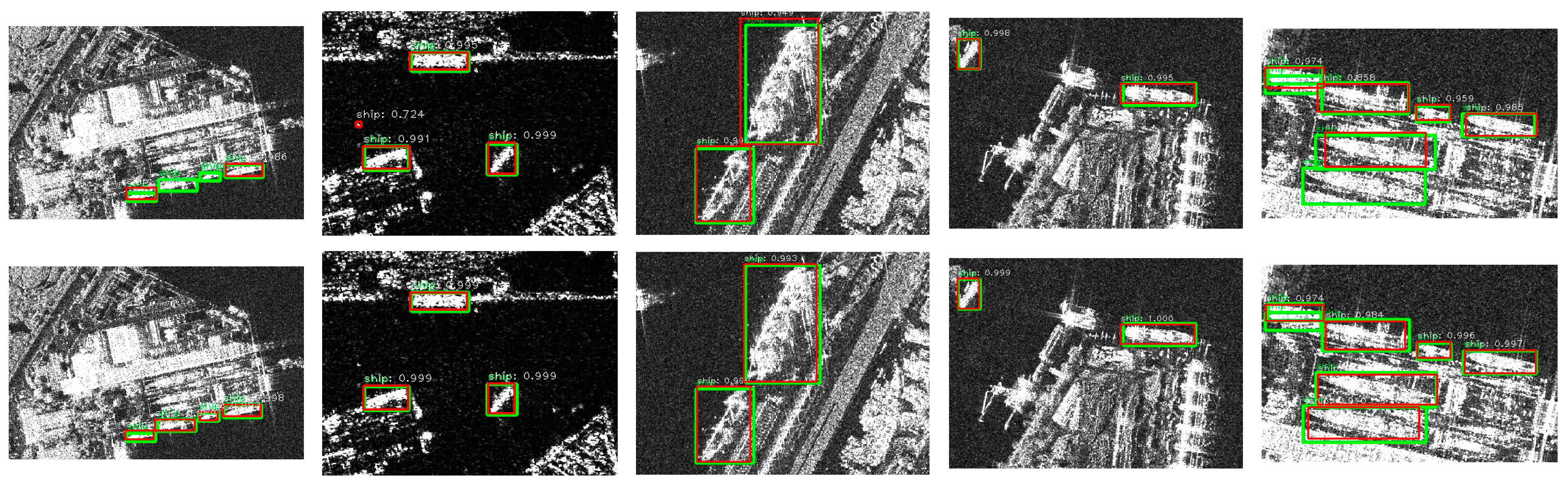
• The HRFPN takes full advantage of the feature maps of high-resolution and low-resolution convolutions for SAR image ship detection. Furthermore, the HRFPN connects high-to-low resolution subnetworks in parallel and can maintain the high resolution. Accordingly, the predicted results are more precise in space compared with FPN, especially inshore and offshore scenes.
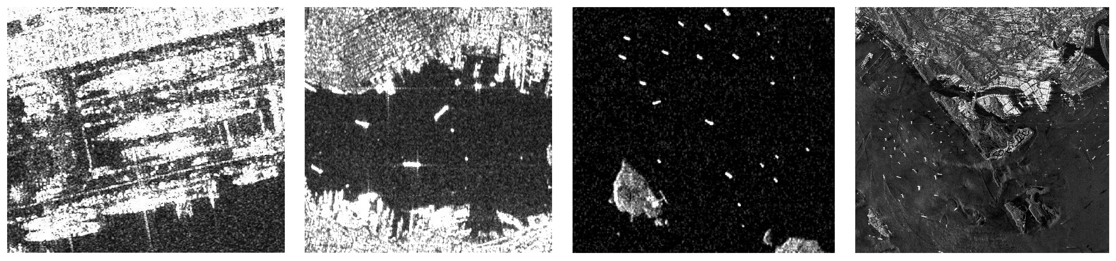
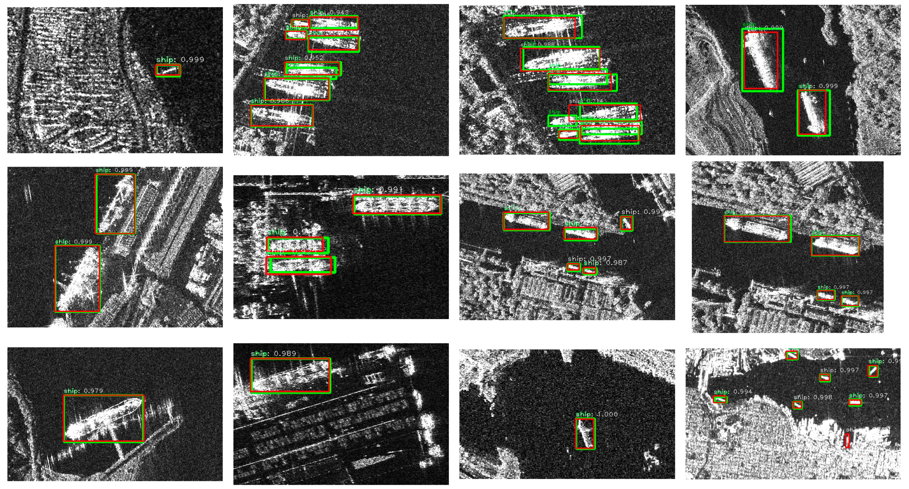
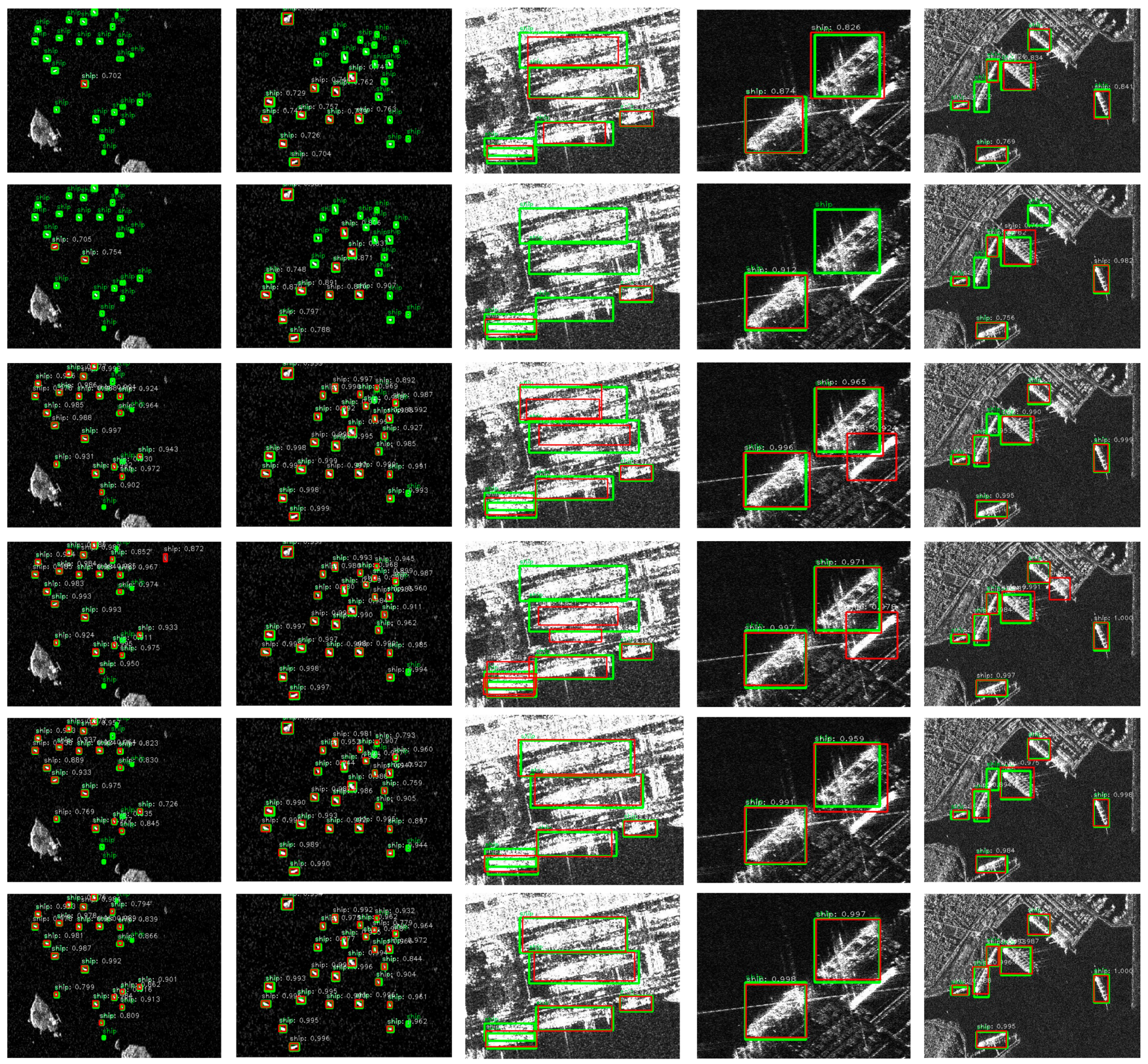
• Our proposed framework HR-SDNet is more accurate and robust than the existing algorithms for ship detection in high-resolution SAR imagery, especially inshore and offshore scenes.
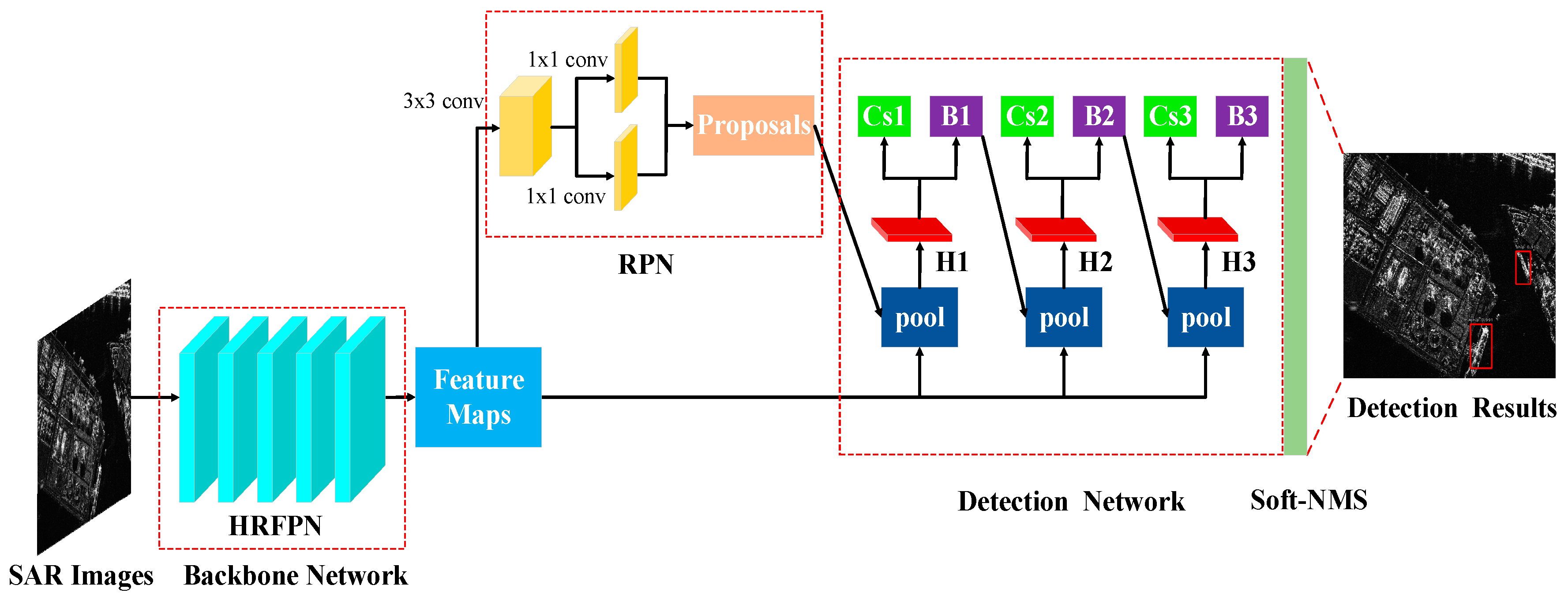
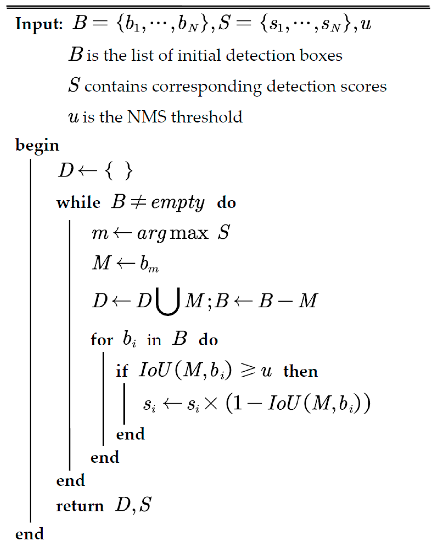
• The Soft-NMS is used to improve the performance of the NMS. It uses the linear penalty function to reduce the detection scores of all other neighbors, thereby improving the detection performance of the dense ships.
• We introduce COCO evaluation metrics to precisely evaluate the detection performance of our method. It contains not only the higher quality evaluation metrics AP but also the evaluation metrics for small, medium, and large targets.
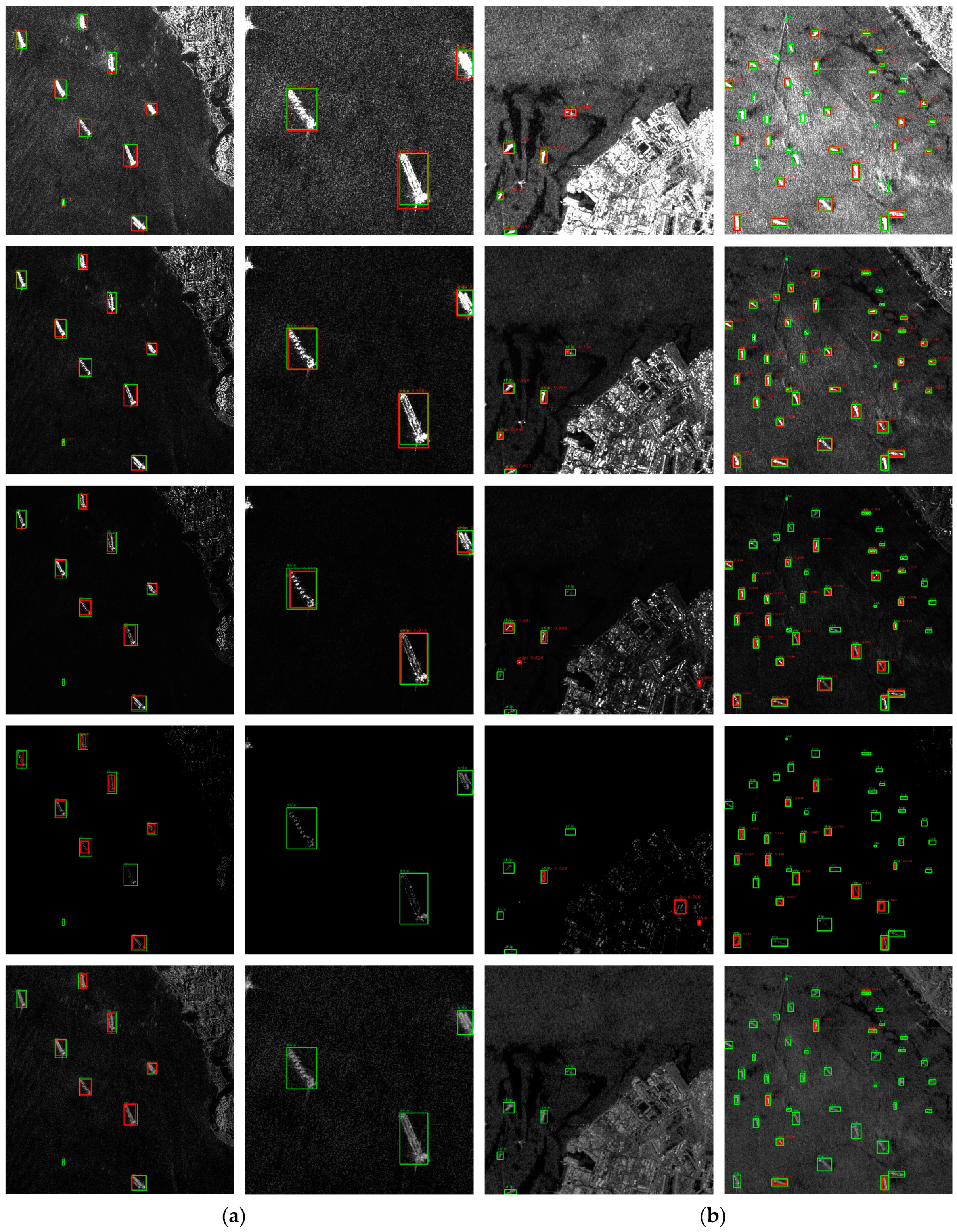
• We analyze the effect of image preprocessing on the robust performance of our detector by the clipping function of the displayed image.

The organization of this paper is as follows. Section 2 relates to the proposed approach. Section 3 reports on the experiments, including the dataset and experimental analysis. Section 4 is a discussion. Section 5 puts up a conclusion and future work.

2. The Methods

In this section, the proposed approach will be expounded in detail.

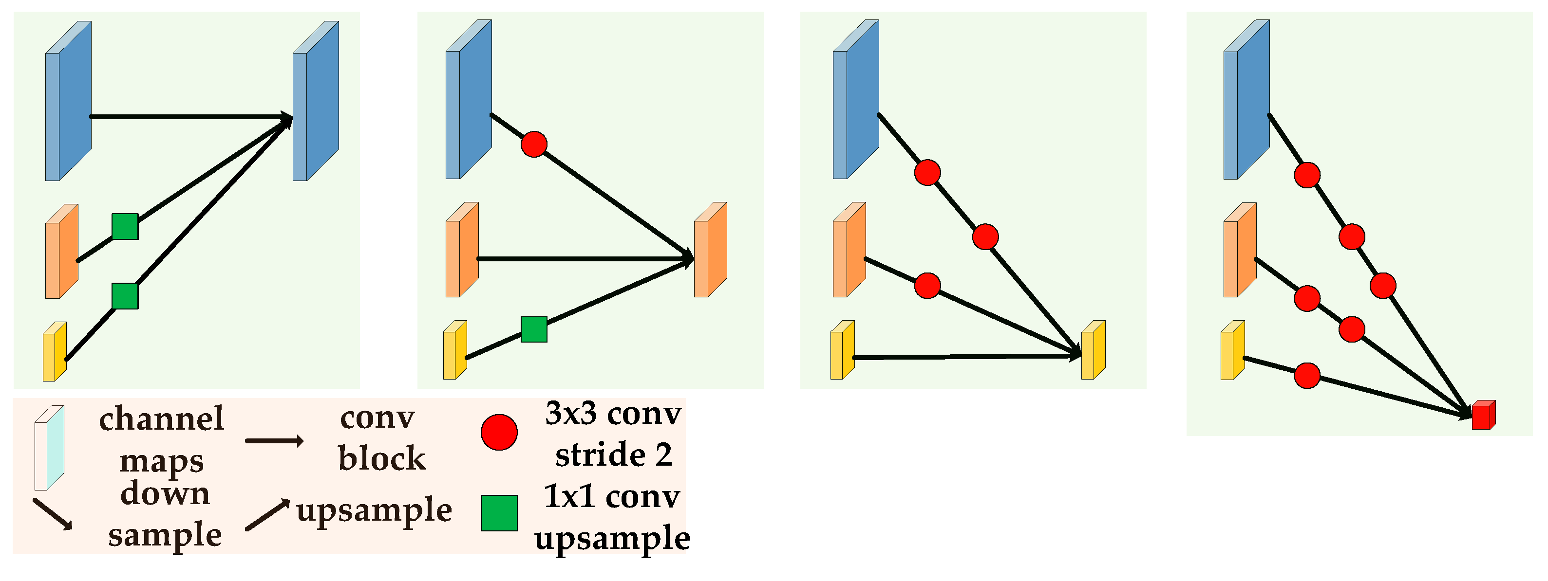
2.1. The Background of HRNet

Visual recognition generally consists of three major research problems: image-level (image classification), region-level (object detection), and pixel-level (including image segmentation, human pose estimation). In recent years, the convolution neural network for image classification has become a standard structure to solve the problem of visual recognition, such as LeNet-5 [45], AlexNet [46], VGGNet [47], GoogleNet [48], ResNet [49], DenseNet [50], etc., as shown by the red line in Figure 2. The characteristic of such networks is that the representation learning gradually becomes smaller in spatial resolution. This network does not apply to visual recognition at the region level and pixel level because the representation learning is characterized by low resolution and the huge loss of resolution makes it difficult to obtain accurate prediction results in spatial accuracy. Therefore, to compensate for the loss of spatial precision, there are two main lines for computing high-resolution. One is to recover high-resolution representations from low-resolution representations. Typical structures include Hourglass [51], U-Net [52], FPN [22], etc., as shown by the green line in Figure 2. The other one is to maintain high-resolution representations through high-resolution convolutions and strengthen the representations with parallel low-resolution convolutions, e.g., high-resolution network (HRNet) [53,54], as shown by the black line in Figure 2.

Although it has a good semantic expression ability, the up-sampling itself cannot completely compensate for the loss of spatial resolution. Therefore, we follow the research line of maintaining high-resolution representations and further study the HRNet, which has achieved promising and remarkable results in human pose estimation [53]. The HRNet always maintains high-resolution feature maps through the whole process of the network, gradually adding low-resolution convolutions, and concatenating multi-resolution convolutions in parallel. At the same time, it improves the expression of high-resolution and low-resolution representations by continuously exchanging information between multi-resolution representations, allowing better mutual promotion between multi-resolution representations. Thus, not only the high-resolution representation is enhanced but also spatially accurate.

2.2. Detailed Description of the Network Architecture

As shown in Figure 3, the high-resolution ship detection network (HR-SDNet) has four components: a high-resolution feature pyramid networks (HRFPN) as the backbone for feature extraction to build a multi-level representation; an region proposal network (RPN) [21] for generating candidate object bounding box proposals; three cascades Fast RCNN with thresholds U = {0.5,0.6,0.7} for bounding box regression and classification; the Soft NMS [38] is executed as a post-processing step to obtain the final ship detection results. Our proposed ship detection framework will be introduced in detail in this section.

2.2.1. Backbone Network

Since HRNet was originally designed for human pose estimation, it cannot be directly applied to ship detection. Hence, the HRNet is modified to make full use of the feature maps of high-resolution and low-resolution convolutions for SAR image ship detection. The resulting network is named as high-resolution feature pyramid networks (HRFPN), as illustrated in Figure 4.

According to Figure 4, the architecture of the HRFPN contains four stages of convolution blocks with four parallel convolution streams and an HRFPN block. The 1st stage includes high-resolution convolutions. The 2nd stage, 3rd stage, and 4th stage repeats two-resolution blocks, three-resolution blocks, and four-resolution blocks, respectively. Starting from a stem, the network is comprised of two strides—2 3 × 3 convolutions which reduce the resolution to ¼ [53,54]. The first stage contains the same four residual units [49,53,54] as ResNet-50, each of which is formed by a bottleneck with a width of 64, and then a 3 × 3 convolution, thereby reducing the number of channels of feature maps to $C_W$. The 2nd, 3rd, and 4th stages are made up of 1, 4, and 3 exchange blocks, respectively. The widths (number of channels) of the convolutions of the four resolutions are $C_W$,2$C_W$4$C_W$.and 8$C_W$ respectively [53,54]. The four stages of convolution blocks have resolutions of $\frac{1}{4}$,$\frac{1}{8}$,$\frac{1}{16}$. and $\frac{1}{32}$, respectively. One exchange block consists of four residual units [49,53,54], each of which contains two 3 × 3 convolutions and an across-the-resolution exchange unit in each resolution. The batch normalization and the nonlinear activation Rectified Linear Unit (ReLU) are performed after each convolution.

Figure 5 is a multi-resolution representation information exchange for three resolution inputs and four resolution outputs. The output representation of each resolution can coalesce the representation of the inputs of the three resolutions to ensure full utilization and interaction of the information. When the high resolution is reduced to the low resolution, we use 3 ×3 convolution with a stride of 2. For up-sampling, the bilinear interpolation is used, and then a 1 × 1 convolution is performed to match the number of channels. Besides, the representations of the same resolution are in the form of identity mapping. The other multi-resolution representation information exchange in the HRFPN is similar to Figure 5.

As shown in Figure 6, we will describe the HRPPN block in the HRFPN in detail. First, we denote the output of the four resolutions from high to low as $\{C_2,C_3,C_4,C_5\}$ and use $\{P_2,P_3,P_4,P_5\}$ to represent newly generated feature maps corresponding to $\{C_2,C_3,C_4,C_5\}$, as shown in Figure 6. Then, the P₂ aggregate the representations of all the up-sampling parallel convolutions. Specifically, the feature maps P₂ are generated through bilinear up-sampling via $C_3,C_4,C_5$, respectively, and concatenate with $C_2$ by 1 × 1 convolution. Finally, each building block takes a higher resolution feature map $P_i$ and a coarser map $C_i$ through lateral connection and generates the new feature map $P_{i+1}$. Each feature map $P_i$ first goes through a 3 × 3 convolution layer with stride 2 to reduce the spatial size. Then each element of feature map $C_i$ that is down-sampled map is added through lateral connection. Where a 1 × 1 convolutional layer is attached to $C_i$. The fused feature map is then processed by another 3 × 3 convolutional layer to generate $P_{i+1}$ for the following a sub-network. This is an iterative process and terminates after approaching $C_5$. Especially, a 1 × 1 convolutional layer is used to reduce the channel dimension in each feature map. All convolutional layers are followed by a ReLU. In these building blocks, we consistently use channel 256 of the feature maps. The feature grid for each proposal is then pooled from new feature maps.

In our experiments, HRFPN consists of one small network, one middle network, and one big network: HRFPN-W18, HRFPN-W32, and HRFPN-W40, where 18, 32, and 40 represent the widths ($C_w$) of the high-resolution subnetworks in the last three stages, respectively. Besides, we reduce the dimension of the high-resolution representation to 144, 256, 320, respectively for HRFPN-W18, HRFPN-W32, and HRFPN-W40 through a 1 × 1 convolution before forming the feature pyramid [53,54]. Therefore, the $C_w$ of the other three parallel subnetworks are 36, 72, 144 for HRFPN-W18, and 64, 128, 256 for HRFPN-W32, and 80, 160, 320 for HRFPN-W40.

2.2.2. Region Proposal Network (RPN)

As shown in Figure 3, RPN consists of a 3 × 3 convolutional layer and two 1 × 1 convolutional layers to generate region proposals for classification and regression. The anchors are used as the reference bounding boxes for classification and regression to generate candidate bounding boxes. Besides, the anchors are of multiple pre-defined scales and aspect ratios to cover ships of different shapes. In this way, the RPN can handle the ship of various sizes and aspect ratios. Following the statistical results in SSDD data sets [35], the anchors can be assigned at different stages based on the anchor size. More specifically, the anchors are assigned five stages $\{{32}^2,{64}^2,{128}^2,{256}^2,{512}^2\}$ to $\{P_2,P_3,P_4,P_5,P_6\}$, respectively. Considering the diverse scales of ships, various aspect ratios $\{1:2,1:1,2:1\}$ are also adopted in each stage. Consequently, there are k = 15 different anchors over the pyramid in total. The 2k confidence scores and 4k outputs encoding the coordinates of k boxes are present in each proposal. Moreover, the ratio of positive and negative samples should be set to $1:3$ to train the entire network.

We assign training labels to the anchors based on their intersection over union (IoU) ratios with ground-truth bounding boxes. Formally, an anchor is assigned a positive label if it has an IoU over 0.7 with any ground-truth box, and a negative label if it has an IoU lower than 0.3 for all ground-truth boxes. Finally, the 2000 region of interest (RoI) is obtained for each image by top-N and Soft-NMS operations on all proposals.

2.2.3. Detection Network

Cascade is a classic yet powerful architecture that has boosted performance on various tasks by multi-stage refinement. Cascade R-CNN [24,39,40] presents a multi-stage architecture for object detection and achieves promising results. The success of Cascade R-CNN can be ascribed to two key aspects: (1) progressive refinement of predictions and (2) adaptive handling of training distributions. Therefore, the cascading structure in Cascade R-CNN is applied to the SAR image ship detection network to improve the quality of ship detection.

The detection network comprises three stages, where the output of each stage is fed into the next one for higher quality refinement. Moreover, the training data of each stage is sampled with increasing IoU thresholds, which handle different training distributions [24]. According to the literature [25,39,40], the output of a detector trained with a certain IoU threshold is a good distribution to train the detector of the next higher IoU threshold. Therefore, the output of one stage is used to train the next stages, which in turn trains the cascade of R-CNN stages. Accordingly, the same cascade procedure is applied to achieve higher ship detection accuracy. Specifically, three cascades of Fast RCNN with thresholds $U=\{0.5,0.6,0.7\}$ [24,39,40] are used to accomplish final ship detection, as is shown in Figure 3. The pooling layer by the RoIAlign [23] is adopted to generate a fixed size of 7 × 7 features. Then, all the 7 × 7 features are flattened and release to fully connected layers for the final ship detection results.

2.2.4. Soft-NMS

Non-Maximum Suppression (NMS) is a significant portion of the ship detection network to predict final ship detections from a set of location candidates, which effectively improves detection performance. The existing detectors exploit a classification sub-network to assign class-specific scores to these proposals while applying a parallel regression sub-network for refining their locations. This refinement process improves the localization accuracy of the ships. Therefore, considering its significant ability to reduce the number of false positives in the final set of detections, the NMS function is of vital importance in state-of-the-art ship detection. [41].

However, zeroing the scores of neighboring detections is the major problem in NMS. In the high-resolution SAR imagery, there are some dense ships in the coastal ports. In general, a ship will be surrounded by other neighboring ships at times; hence, the bounding boxes of nearby ships may appear in that overlap threshold. Therefore, the ship’s bounding boxes will be lost, and the average precision will be decreased. Instead of eliminating all the lower scores surrounding bounding boxes, to address this problem, Soft Non-Maximum Suppression (Soft-NMS) [41] uses the linear penalty function to reduce the detection scores of all other neighbors, which is denoted as follows [41]:

$$s_i=\{\begin{array}{c}{s}_i,\begin{array}{cccc}\begin{array}{ccc}& & \end{array}& & & \end{array}IoU\left(M,b_i\right)<u\hfill \\ s_i\times \left(1-IoU\left(M,b_i\right)\right),IoU\left(M,b_i\right)\ge u\end{array}.$$

(1)

where s_i is the detection scores; M indicates the maximum score detection box; $b_i$ represents the detection box in the remaining detection boxes; $IoU(M_i,b_i)$ calculates intersection-over-union between two detection boxes; $u$ denotes $IoU$ threshold. The pseudo-code of the Soft-NMS algorithm is presented in Figure 7 [41].

2.3. Loss Function

For an image, the overall loss function is as follows [20,24]:

$$L=R_{cls}\left[h\right]+\lambda \left[y⩾1\right]R_{loc}\left[f\right].$$

(2)

where is the parameter to balance the loss of classification and regression. All experiments use $\lambda =1$. $\left[y⩾1\right]$ is the Iverson bracket indicator function [20]. When $\left[y⩾1\right]$ the function equals to 1, otherwise it equals to 0.

• Bounding box regression

$b=\left(b_x,b_y,b_w,b_h\right)$ and $g=\left(g_x,g_y,g_w,g_h\right)$ can denote the predicted bounding box and ground-truth bounding box, respectively, which contains the four coordinates of an image patch $x$. Bounding box regression uses the regressor $f\left(x,b\right)$ to regress a candidate bounding box $b$ into a target bounding box $g$ [24,39]. This is learned from a training set $\left(g_i,b_i\right)$, by minimizing the risk.

$$R_{loc}\left[f\right]={\displaystyle \sum _i{L}_{loc}}\left(f\left(x_i,b_i\right),g_i\right).$$

(3)

As in Fast R-CNN [20],

$$L_{loc}\left(g,b\right)={\displaystyle \sum _{j\in \left\{x,y,w,h\right\}}smoot{h}_{L_1}}\left(g_j-b_j\right).$$

(4)

where

$$smoot{h}_{L_1}\left(x\right)=\{\begin{array}{c}0.5x^2,\left|x\right|<1\\ \left|x\right|-0.5,otherwise\end{array}.$$

(5)

is the smooth L₁ loss function. To encourage invariance to scale and location, $smoot{h}_{L_1}$ operates on the distance vector $\Delta =\left({\delta }_x,{\delta }_y,{\delta }_w,{\delta }_h\right)$ defined by [20,21,24]

$$\begin{array}{l}{\delta }_x=\left(g_x-b_x\right)/b_w,{\delta }_y=\left(g_y-b_y\right)/b_h\\ {\delta }_w=\log \left(g_w/b_w\right),{\delta }_h=\log \left(g_h/b_h\right)\end{array}$$

(6)

In addition, $\Delta =\left({\delta }_x,{\delta }_y,{\delta }_w,{\delta }_h\right)$ needs to be normalized by its mean and variance [20,21].

• Classification

The function $h\left(x\right)$ which is the classifier can assign an image patch $x$ to one of $M+1$ categories, where class 0 contains background and the remaining denotes the object detection categories. The posterior distribution over classes is $h\left(x\right)$, i.e., $h_k\left(x\right)=p\left(y=k|x\right)$, where $y$ is the categories label. Given a training set $\left(x_i,y_i\right)$, the classification risk can be minimized as follows:

$$R_{cls}\left[h\right]={\displaystyle \sum _i{L}_{cls}}\left(h\left(x_i\right),y_i\right).$$

(7)

where

$$L_{cls}\left(h\left(x\right),y\right)=-\log h_y\left(x\right)$$

(8)

is the cross-entropy loss.

3. Experiments and Results

In this section, we will evaluate the ship detection approach for high-resolution SAR imagery. We not only compare the ship detection performance in terms of average precision (AP) [42], and the visualization results, but also test the robustness of our proposed method.

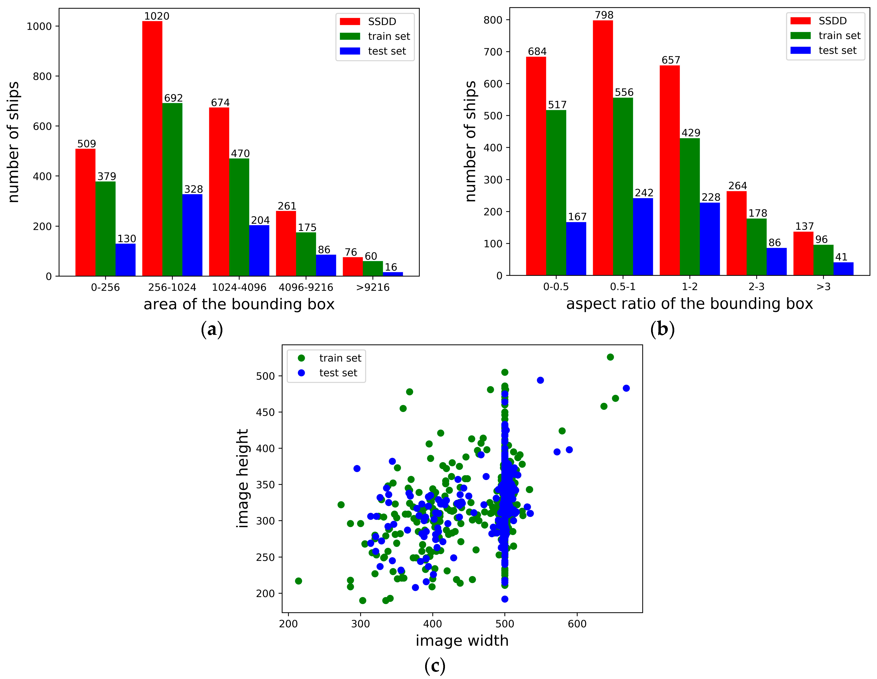
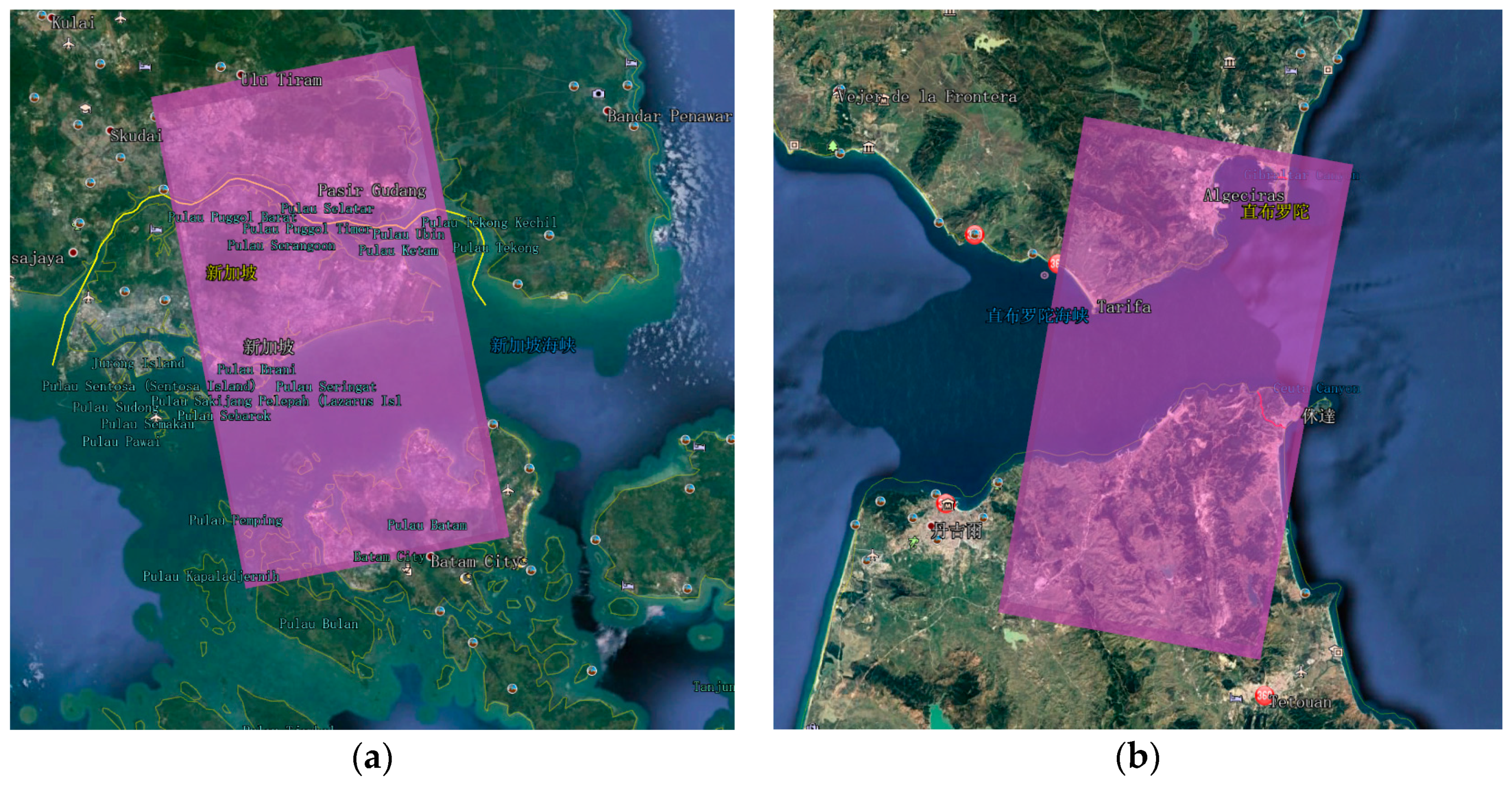
3.1. Dataset Description

The SAR ship detection dataset (SSDD) data sets [35] are used in the experiments. The SSDD dataset draws on the construction process of The Pascal Visual Object Classes (PASCAL VOC) datasets [55], including SAR images with different resolutions, polarizations, sea conditions, large sea areas, and beaches. This dataset is a benchmark for researchers to evaluate their approaches. In SSDD, there are 1160 images and 2540 ships in total. The average number of ships per image is 2.12. For SSDD, the resolution of SAR images is as follows: 1 m, 3 m, 5 m, 7 m, and 10 m. The diversity of the resolution ensures better adaptability in the trained model. Polarization is also diverse. Figure 8 gives a statistical analysis of the SSDD data set. According to the reference [56], the area of the bounding box is divided into five levels: extra-small (S_b < 16² pixels), small (${16}^2$<$s^2$<${32}^2$ pixels), middle (${32}^2$<$s_b$<${64}^2$ pixels), large (${64}^2$<$s_b$<${96}^2$ pixels), and extra-large (pixels), where $s_b$ is the number of pixels in each bounding box. As can be observed, much of the bounding box is on a small and middle scale. The aspect ratio of the bounding box is also divided into five levels, and over 84.20% of them are distributed in 0.5–2. The distribution of the aspect ratio can provide essential information for anchor-based models. What is more, it is easy to resize the image due to the width and height of the statistical image to process the image in batches.

Furthermore, to provide further confirmation, the previous models are evaluated on two real SAR images from the Strait of Singapore and the Strait of Gibraltar. The SAR imagery was acquired from the TerraSAR-X sensor [44], which has a resolution of 3 m. In order to analyze the inshore and offshore scenes, we intercept areas of size 10269 × 6365, 10269 × 6365 in the Singapore Strait and Gibraltar Strait, respectively. Detailed descriptions of two high-resolution SAR imagery are shown in

Table 1. The Information about the TerraSAR-X Imagery.

Satellite	Waveband	Polarization	Resolution	Time	Position	Imaging Mode
TerraSAR	X	HH	3 m	2010-05-17	Strait of Singapore	Strip Map
TerraSAR	X	HH	3 m	2008-05-12	Strait of Gibraltar	Strip Map

and Figure 9.

3.2. Evaluation Metrics

To quantitatively evaluate the performance and robustness of the proposed frameworks, the following metrics are widely used: intersection over union (IoU), precision, recall, and mean average precision (mAP). As shown in formula (12), IoU is the overlap rate of the predict bounding box and ground-truth generated by the model. The calculation formulas of precision and recall are as follows:

$$Precision=\frac{TP}{TP+FP},$$

(9)

$$Recall=\frac{TP}{TP+FN}.$$

(10)

where TP (True Positives) indicates the number of correctly detected ships; FN (False Negatives) denotes the number of non-detected or missed ships; and FP (False Positives or false alarms) represents the number of incorrectly detected ships.

For single class target ship detection, mean average precision (mAP) is defined by [55]:

$$mAP={\displaystyle {\int }_0^{1}P\left(r\right)}dr,$$

(11)

where r represents recall and $P(r)$ denotes the precision value that recall = r corresponds to. For ship detection, the larger the value of mAP is, the better the detection performance of the ship is.

However, the mean average precision (mAP) does not fully reflect the performance of the object detection framework. Compared to the mAP of PascalVOC [55], the Microsoft Common Objects in Context (COCO) [42] includes not only the higher quality evaluation metrics, such as AP, AP₅₀, and AP₇₅ for more accurate bounding box regression, but also the evaluation metrics AP_L, AP_M, and AP_S for large, medium, and small objects. Thus, COCO metrics are more objective and comprehensive for object detection tasks.

In general, mAP is a default metric of precision in the PascalVOC competition [55], which is the same as AP₅₀ [42] metric in the MS COCO competition. Besides, COCO metrics are standard and widely used evaluation metrics in object detection tasks.

$$IoU\left(B_p,B_g\right)=\frac{B_p\cap B_g}{B_p\cup B_g},$$

(12)

For SAR ship detection, we leverage the standard COCO [42] metrics to quantitatively evaluate the performance of the proposed framework, including AP, AP₅₀, AP₇₅, AP_S, AP_M, AP_L [42]. As can be seen from

Table 2. COCO Dataset Object Detection Evaluation Metrics [42].

Metrics	Metrics Meaning
AP	AP at IoU = 0.50: 0.05: 0.95
AP50	AP at IoU = 0.50
AP75	AP at IoU = 0.75
APS	AP for small objects: area < 322
APM	AP for medium objects: 322 < area < 962
APL	AP for large objects: area > 962

, AP₅₀ denotes the set threshold of IoU as 0.50; AP₇₅ denotes that the threshold is set as 0.75; AP indicates that the threshold of IoU is set from 0.50 to 0.95, where the step size is 0.05; AP_S is set for small objects in which the area is smaller than ${32}^2$; AP_M is set for medium objects in which the area is between ${32}^2$ and ${96}^2$; AP_L is set for large objects in which the area is bigger than ${96}^2$. The larger the value of AP is, the more accurate the prediction results in spatial accuracy are, and the better the detection performance of the ship is. For AP₅₀, when the IoU of the ground-truth and the predicted box is greater than 0.5, the test case is predicted as a ship. Therefore, with a higher IoU threshold, the bounding box regression will be better and the ship is well covered by the predicted bounding box. So AP₇₅ evaluates the accuracy of the bounding box regression better than AP₅₀. The larger the value of AP₇₅ is, the more accurate the predicted bounding box is.

3.3. Implementation Details

For the sake of fair comparison, the experiments and comparisons are implemented on mmdetection [57], which is a well-known open-source deep learning framework and executed on a personal computer (PC) with an Intel(R) i7-8700 CPU @3.20GHz, NVIDIA GTX-1080Ti GPU (11 GB memory), and 64 GB RAM. The PC operating system is a 64-bit Ubuntu 16.04. In our experiment, the SSDD data set is randomly divided into two parts: 70% for the training data set and 30% for the testing data set. In order to validate our approach comprehensively and avoid overfitting, we expanded our dataset by rotating and flipping the image to enhance the number of data sets.

3.3.1. Implementation Details of HR-SDNet

In our experiments, HRFPN consists of one small network, one middle network, and one big network: HRFPN-W18, HRFPN-W32, and HRFPN-W40, respectively, as the backbone network extraction features. The detection head of all baseline detectors in the HR-SDNet detection network has the same architecture, which is composed of three cascades of Fast RCNN with thresholds $U=\{0.5,0.6,0.7\}$ for bounding boxes regression and classification. The IoU threshold of the Soft-NMS is set to 0.5. The inference is made on a single image scale with no further bells and whistles.

We train detectors with GPUs for 20 epochs with an initial learning rate of 0.0025, and decrease it by 0.1 after 16 and 19 epochs respectively, on one GPU of batch size two images. The weight decay and momentum are set to 0.0001 and 0.9, respectively. Furthermore, we use SGD to optimize the model. The input images by the bilinear interpolation are resized to have 600px along the short axis and a maximum of 1000 px along the long axis for training and testing. The entire detector uses multi-task loss. In addition, the entire network is end-to-end training as a whole. For other parameters, we follow the hyperparameter setting in reference [39,40,57,58].

3.3.2. Compared Approaches

To test the performance of HR-SDNet, the comparative experiments were implemented using multiple popular single-model baselines: Faster R-CNN [21], RetinaNet [31], Mask R-CNN [23] and Cascade R-CNN [24] with ResNet-FPN [58] backbone or ResNext -FPN [59] backbone, YOLOv2 [25] with Darknet-19, for the task of ship detection. These baselines have a wide range of performance. We use its default settings unless otherwise noted and use the end-to-end training for the entire detector. Faster R-CNN, RetinaNet, Mask R-CNN, and Cascade R-CNN use the same parameter settings [25,39,40]. Besides, the YOLOv2 generates five anchors by k-means clustering, the anchor setting of other models is consistent with the HR-SDNet proposed in this paper.

We train the detectors with a GPU for 12 epochs with an initial learning rate of 0.0025 and decrease it by 0.1 after eight and 11 epochs, respectively. The weight decay and momentum are set to 0.0001 and 0.9, respectively. The input images by the bilinear interpolation are resized to have 600 px along the short axis and a maximum of 1000 px along the long axis for training and testing. For other parameters, we follow the hyperparameter setting in reference [57].

3.4. Experimental Results and Analysis of HR-SDNet

3.4.1. Effect of the HRFPN

The comparison results of FPN and HRFPN in the inshore and offshore scenes are shown in Figure 10. We use Cascade R-CNN as a strong baseline to implement our method and a comparison method. In complex inshore scenes, FPN has more missed ships. Compared with FPN, the HRFPN is more accurate in the bounding box regression. It is worth noting that the ship detection performance of the HRPFN is superior to the original FPN and provides a very powerful baseline, whether inshore or offshore scenes.

As can be observed from the results in

Table 3. Effect of the HRFPN in the Inshore and Offshore Scenes.

Backbone	Param (M)	Test Speed	Scenes	AP	AP50	AP75	APS	APM	APL
ResNet-50+FPN	552.6	0.099s	Inshore	46.7	80.6	48.4	40.1	53.5	51.3
			Offshore	64.8	98.6	76.0	59.2	74.2	63.4
ResNet-101+FPN	704.8	0.112s	Inshore	47.9	83.8	46.7	40.1	53.5	51.3
			Offshore	64.7	98.7	76.4	59.4	73.4	60.1
ResNext-101+64x4d+FPN	1024.0	0.164s	Inshore	49.3	85.1	48.7	41.3	56.4	60.2
			Offshore	65.8	98.4	75.7	60.1	74.7	63.5
HRFPN-W18	439.7	0.083s	Inshore	50.7	84.7	54.2	42.6	57.8	66.3
			Offshore	66.1	98.7	76.7	60.2	75.8	60.1
HRFPN-W32	598.1	0.095s	Inshore	51.0	84.6	54.0	42.5	57.5	67.3
			Offshore	66.4	98.7	79.0	60.6	75.1	63.4
HRFPN-W40	728.2	0.103s	Inshore	53.6	88.7	56.9	46.1	59.6	74.8
			Offshore	66.6	98.8	79.5	60.5	75.0	60.6

, the HRFPN performs better than FPN, with smaller parameters and less computational complexity in the cascade R-CNN framework, especially for inshore or offshore scenes. Looking at the various indicators in offshore scenes, except for the significant improvement of AP₇₅, the remaining indicators have not improved much, indicating that HRFPN is more accurate than FPN for bounding box regression under the same detection capability. Moreover, the AP value is 53.6% for inshore scenes, which achieves nearly 4.3% performance gains compared to FPN. It is shown that our method significantly improves the ship detection performance for inshore scenes and obtains more accurate prediction results in spatial accuracy. The AP₅₀ and AP₇₅ values are 88.7%, 56.9% for inshore scenes, compared to FPN, which achieves a gain of 3.6%, 8.2%, respectively. The results show that the bounding box regression will be better and more accurate. For AP_S, AP_M, AP_L, they have also been significantly improved. It is shown that the detection performance has been significantly improved for small, medium, and large ships in inshore scenes. Therefore, HRFPN is effective.

In the HRFPN structure, compared with HRFPN-W18 and HRFPN-W32, our HRFPN-W40 has better performance, but it also increases the parameters and computational complexity.

In summary, the HRFPN, which maintains the high resolution and takes full advantage of the feature maps of the high-resolution and low-resolution convolutions, can effectively improve the ship detection performance for SAR images and makes the predicted results more accurate in space, especially for inshore or offshore scenes. Therefore, HRFPN is effective.

3.4.2. Results of the HR-SDNet

The ship detection results of the proposed method in the inshore and offshore scenes are shown in Figure 11. The red box indicates the prediction result, and the green box indicates the ground-truth. It can be seen from Figure 11; the HR-SDNet has superior detection performance for both inshore and offshore scenes of the high-resolution SAR imagery.

As can be seen from

Table 4. Results on SSDD for HR-SDNet which use NMS as a Baseline and the Soft-NMS Method.

Backbone	Method	AP	AP50	AP75	APS	APM	APL
ResNet-50+FPN	NMS	61.3	95.6	70.7	56.5	69.0	53.0
	Soft-NMS	62.7	96.2	73.4	57.6	70.5	56.9
ResNet-101+FPN	NMS	61.4	96.0	70.4	56.7	68.1	68.3
	Soft-NMS	62.7	96.7	71.9	57.7	69.6	70.0
ResNext-101+64x4d+FPN	NMS	62.8	96.5	70.3	57.3	70.3	61.6
	Soft-NMS	63.9	96.5	72.9	58.4	71.6	64.1
HRFPN-W18	NMS	63.0	96.1	72.1	57.3	71.4	63.0
	Soft-NMS	63.9	96.8	73.1	58.2	72.3	65.0
HRFPN-W32	NMS	63.5	96.3	74.3	58.0	71.0	66.1
	Soft-NMS	64.5	97.0	76.0	58.8	72.0	67.7
HRFPN-W40	NMS	63.7	97.3	74.3	58.3	71.2	70.6
	Soft-NMS	64.6	97.9	75.9	59.0	72.3	72.0

, the proposed network, based on HRFPN-W18, HRFPN-W32, and the HRFPN-W40 backbone, has the best performance, which achieves a gain of 1.7%, 2.1%, and 0.9% in terms of AP for ResNet-50+FPN, ResNet-101+FPN, and ResNext-101+64x4d+FPN, respectively. It is shown that our method improves the ship detection performance and obtains more accurate the prediction results in spatial accuracy. Moreover, The AP₇₅ value of HRFPN-W18, HRFPN-W32, and HRFPN-W40 backbone are 72.1%, 74.3%, 74.3%, respectively, which achieves a gain of 1.4%, 3.9%, 4% for ResNet-50+FPN, ResNet-101+FPN, and ResNext-101+64x4d+FPN, respectively. The AP₅₀ has also been greatly improved. The results show that the bounding box regression will be better, and the ship is well covered by the predicted bounding box. For AP_S, AP_M, AP_L, they have also been significantly improved. It is shown that the detection performance has been improved for small, medium, and large ships. In the HRFPN structure, our HRFPN-W40 performance is better with the AP value of 63.7%, compared to HRFPN-W18 and HRFPN-W32, which bring 0.7% and 0.2% gain in terms of AP, respectively. Therefore, it can be inferred that the proposed HRFPN modules play an important role in improving detection performance, especially satisfying the detection results for the ships.

In addition, some ships are closely aligned and dense in coastal ports, and the IoU of their bounding boxes easily reach the overlap threshold, which causes adjacent ships to be suppressed in NMS. Hence, Soft-NMS is used to improve the performance of the NMS. With the Soft-NMS algorithm, our network performs better, which achieves nearly 1% performance gains in terms of AP in Table 4. It can be seen from Table 4 that our model with Soft-NMS can significantly improve AP, thus improving the detection performance of neighboring ships and demonstrating its effectiveness.

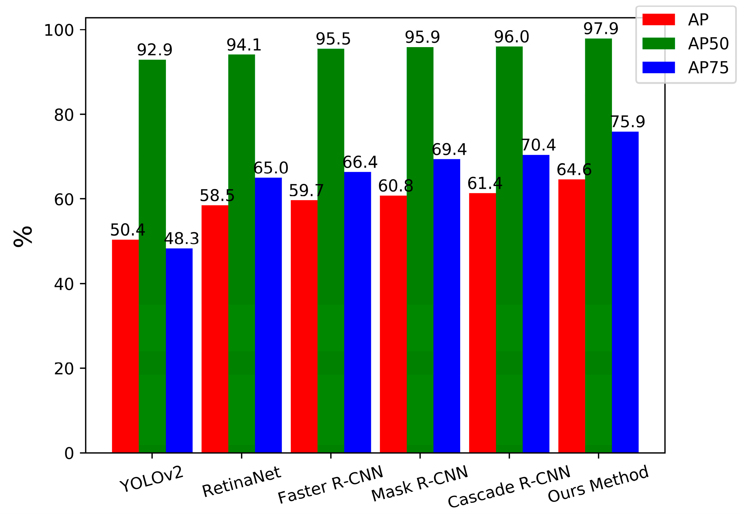
3.5. Comparison with the State-of-the-Art

To further demonstrate the detection performance of the proposed network, the qualitative results between our approach and the five compared methods are shown in Figure 12, where the green boxes denote the ground-truth of the ship, the red boxes indicate the predicted results of ship detection. Row 1 is the ship detection results of YOLOv2; Row 2 is the ship detection results of RetinaNet; Row 3 is the ship detection results of Faster R-CNN; Row 4 is the ship detection results of Mask R-CNN; Row 5 is the ship detection results of Cascade R-CNN; Row 6 is the ship detection results of HR-SDNet. Column 1 and Column 2 is the offshore scenes; Others are the inshore scenes.

As shown in Figure 12, compared to the state-of-the-art single-model detectors, our method can accurately detect the ships in a different scene. Specifically, the ship is covered well with predicted bounding boxes. For closely aligned and dense ships in coastal ports, our method gets a great detection performance improvement. For small ships in the offshore scenes, YOLOv2 and RetinaNet have more missed ships, and our method can accurately detect the ships because the network is able to learn enough high-resolution representations successfully. Compared to Faster R-CNN and Mask R-CNN, our approach has almost no false alarm. Compared to Cascade R-CNN, our approach is more accurate in the bounding box regression. The results on the SAR ship SSDD dataset reveal that our approach is practical for ship detection of high-resolution SAR imagery and achieves a better ship detection performance than the existing approaches.

To quantitatively evaluate the performance of the proposed models, the HR-SDNet, based on HRFPN backbone and the Soft-NMS algorithm, is compared with the state-of-the-art single-model ship detectors on the SSDD data set in

Table 5. Comparison with state-of-the-art Single-Model Detectors in the SSDD Data Set.

Model	Backbone	Param (M)	Test Speed	AP	AP50	AP75	APS	APM	APL
YOLOv2	Darknet-19	197.0	0.020s	50.4	92.9	48.3	52.4	52.5	54.9
RetinaNet	ResNet-50+FPN	290.0	0.075s	58.5	94.1	65.0	54.2	65.8	52.0
RetinaNet	ResNet-101+FPN	442.3	0.078s	58.3	93.8	65.5	54.0	65.5	55.0
Faster R-CNN	ResNet-50+FPN	330.2	0.063s	59.5	96.2	67.0	55.5	66.3	46.9
Faster R-CNN	ResNet-101+FPN	482.4	0.075s	59.7	95.5	66.4	55.3	66.3	48.1
Mask R-CNN	ResNet-50+FPN	351.2	0.069s	60.5	96.3	70.0	56.7	67.4	47.9
Mask R-CNN	ResNet-101+FPN	503.4	0.080s	60.8	95.9	69.4	56.0	68.6	49.0
Cascade R-CNN	ResNet-50+FPN	552.6	0.099s	61.3	95.6	70.7	56.5	69.0	53.0
Cascade R-CNN	ResNet-101+FPN	704.8	0.112s	61.4	96.0	70.4	56.7	68.1	68.3
HR-SDNet	HRFPN-W18	439.7	0.083s	63.9	96.8	73.1	58.2	72.3	65.0
HR-SDNet	HRFPN-W32	598.1	0.095s	64.5	97.0	76.0	58.8	72.0	67.7
HR-SDNet	HRFPN-W40	728.2	0.103s	64.6	97.9	75.9	59.0	72.3	72.0

. The first group of detectors in Table 5 is one-stage detection algorithms; the second group is two-stage detection algorithms, and the last group is multi-stage detection algorithms. The HR-SDNet outperformed all single-model detectors by a large margin, under all evaluation metrics. This includes the single-model entries of YOLOv2 [26], RetinaNet [31], Faster R-CNN [21], Mask R-CNN [23] and Cascade R-CNN [24]. For a better understanding of Table 5, we visualize the results using a bar chart in Figure 13, where the red, green and blue bar chart represents AP, AP_50, and AP₇₅ of the state-of-the-art single-model detectors, respectively.

As can be seen from Table 5 and Figure 13, the proposed approach has the best performance with the AP value of 64.6%. Compared with YOLOv2 and RetinaNet, the HR-SDNet achieves gains of 14.2% and 6.1%, respectively. Compared with Faster R-CNN, Mask R-CNN, and Cascade R-CNN, the HR-SDNet achieves gains of 4.9%, 3.8%, and 3.2%, respectively. As a consequence, our method has better detection performance, and more accurate prediction results in spatial accuracy than other ship detection methods on SSDD. Additionally, the AP₅₀ value of HR-SDNet is 97.9%, which achieves nearly 2% performance gains. The AP₇₅ value of HR-SDNet is 75.9%, which achieves a gain of 8.9%, 5.9%, and 5.2% for Faster R-CNN, Mask R-CNN, and Cascade R-CNN, respectively. Compared with YOLOv2 and RetinaNet, the HR-SDNet achieves gains of 27.6% and 10.4%, respectively. The results show that the bounding box regression will be better and more accurate than the existing algorithms for ship detection. For small, medium, and large ships, compared with other detection algorithms, the HR-SDNet has also been significantly improved in terms of AP_S, AP_M, AP_L. Among them, the performance improvement of large ships is the most obvious. Compared to one-stage, two-stage, and multi-stage detection algorithms, HR-SDNet achieves a gain of 17%, 23%, and 3.3% in terms of AP_L, respectively. It implies that HRFPN can greatly improve the detection performance and is effective.

As can be seen from Table 5, compared to one-stage, two-stage detection algorithms, our models have better performance, but it also increases the parameters and computational complexity. Additionally, the HR-SDNet performs better than Cascade R-CNN, with smaller parameters and less computational complexity. Therefore, it also proves the advantages of our network.

Figure 12 and Table 5 can reflect that the higher the AP, AP₅₀, and AP₇₅, the better the performance of the ship detector, and the more accurate the predicted bounding boxes. The higher the AP_S, AP_M, and AP_L are, the better detection performance for small, medium, and large ships is. It shows that the COCO evaluation metrics are effective for SAR image ship detection.

As can be seen from

Table 6. Comparison with the state-of-the-art Single-Model Detectors in the Inshore and Offshore Scenes on the SSDD Data Set.

Model	Backbone	Scenes	AP	AP50	AP75	APS	APM	APL
Faster R-CNN	ResNet-50+FPN	Inshore	43.2	79.0	42.1	36.6	51.8	43.2
		Offshore	63.1	98.6	73.3	58.4	70.9	60.0
	ResNet-101+FPN	Inshore	44.5	79.8	42.0	37.8	51.6	47.9
		Offshore	63.0	97.7	72.5	58.1	71.1	55.0
Mask R-CNN	ResNet-50+FPN	Inshore	45.0	79.8	43.7	37.8	53.7	44.8
		Offshore	63.9	98.7	76.3	59.7	71.5	60.1
	ResNet-101+FPN	Inshore	44.6	77.6	45.4	38.8	50.7	45.3
		Offshore	64.3	98.5	74.8	58.6	73.6	60.1
Cascade R-CNN	ResNet-50+FPN	Inshore	46.7	80.6	48.4	40.1	53.5	51.3
		Offshore	64.8	98.6	76.0	59.2	74.2	63.4
	ResNet-101+FPN	Inshore	47.9	83.8	46.7	40.1	53.5	51.3
		Offshore	64.7	98.7	76.4	59.4	73.4	60.1
DAPN [1]	DFPN-CON	Inshore	-	67.5	-	-	-	-
		Inshore	-	95.9	-	-	-	-
HR-SDNet	HRFPN-W18	Inshore	50.7	84.7	54.2	42.6	57.8	66.3
		Offshore	66.1	98.7	76.7	60.2	75.8	60.1
	HRFPN-W32	Inshore	51.0	84.6	54.0	42.5	57.5	67.3
		Offshore	66.4	98.7	79.0	60.6	75.1	63.4
	HRFPN-W40	Inshore	53.6	88.7	56.9	46.1	59.6	74.8
		Offshore	66.6	98.8	79.5	60.5	75.0	60.6

, the AP value of HR-SDNet is 53.6% for inshore scenes, which achieves a gain of 9.1%, 8.6%, and 5.7% for Faster R-CNN, Mask R-CNN, and Cascade R-CNN, respectively. As a consequence, compared with other ship detection methods on SSDD, our method significantly improves the ship detection performance for inshore scenes and obtains more accurate prediction results in spatial accuracy. Additionally, the AP₅₀ value of HR-SDNet is 88.7%, which achieves a gain of 8.9%, 8.9%, and 4.9% for Faster R-CNN, Mask R-CNN, and Cascade R-CNN, respectively. The AP₇₅ value of HR-SDNet is 56.9%, which achieves a gain of 14.8%, 11.5%, and 8.5% for Faster R-CNN, Mask R-CNN, and Cascade R-CNN, respectively. The show that the bounding box regression will be better and more accurate than the existing algorithms for ship detection in inshore scenes. For small, medium, and large ships, compared with other detection algorithms, the HR-SDNet achieves nearly 6–8%, 6–7%, and 23–26% performance gains in terms of AP_S, AP_M, AP_L, respectively. Among them, the performance improvement of large ships is the most obvious. It is shown that the detection performance has been significantly improved for small, medium, and large ships in inshore scenes. Looking at the various indicators in offshore scenes in Table 6, except for the significant improvement of AP and AP₇₅, the remaining indicators have not improved much, indicating that our method is more accurate than other ship detection methods for bounding box regression. Compared with the Dense Attention Pyramid Networks (DAPN) [1] proposed by Cui et al., our method performs better and achieves a gain of 21.2% in terms of AP₅₀ for inshore scenes. It implies that HRFPN can greatly improve the detection performance and is effective.

In summary, compared to the state-of-the-art single-model detectors, our method based on HRFPN significantly improves the ship detection performance in SAR images and obtains more accurate prediction results in spatial accuracy, especially for inshore or offshore scenes. This is because the HRFPN maintains the high resolution and takes full advantage of the feature maps of high-resolution and low-resolution convolutions. At the same time, it also shows that the COCO evaluation metrics are effective for SAR image ship detection.

3.6. Robustness Analysis

In SAR image processing, the image is generally displayed by a clipping function after processing the SAR image. To analyze the effect of image preprocessing on the robust performance of our detector, we define the clipping function of the image displayed. The clipping function is divided into linear and logarithmic changes, which is denoted as follows:

$$y=\{\begin{array}{c}kx,0<x⩽\beta \times \max \left(x\right)\\ \beta \times \max \left(x\right),x>\beta \times \max \left(x\right)\end{array}$$

(13)

$$y=\{\begin{array}{c}In\left(x\right),In\left(x\right)⩾\alpha \\ \alpha ,In\left(x\right)<\alpha \end{array}$$

(14)

where $k$ indicates the penalty factor and we set $k=1$. x and y represent input and output images, respectively. We follow the hyperparameter setting in the literature [43]. We set $\alpha =-20dB,-30dB$,$\beta =0.008,0.02,0.05$.

In this paper, the SAR images from the Strait of Singapore and the Strait of Gibraltar are annotated by the LabelMe open source project on GitHub [60,61,62,63], which is currently the most widely used annotation tool. In the annotation, some targets are very small and only a few pixels, and it is difficult for the naked eye to distinguish between ships and speckle noise. Therefore, we consider the number of pixels greater than 10 as the ship’s pixels and label them.

Figure 14 shows the ship detection results in the TerraSAR-X test image. These SAR images are partial images of the Singapore Strait and Gibraltar Strait. Row 1 is the result of 0.008; Row 2 is the result of 0.02; Row 3 is the result of 0.05; Row 4 is the result of −20 dB; Row 5 is the result of −30 dB. Red boxes denote predicted results; green boxes denote ground-truth.

As can be seen from Figure 14 and

Table 7. Quantitative results of ship detection in the TerraSAR-X test images. Where TP indicates the number of correctly detected ships; FN denotes the number of non-detected or missed ships; and FP represents the number of incorrectly detected ships.

Threshold	Ground Truth	TP	FN	FP	Recall	Precision
0.008	58	44	14	0	75.86%	100%
0.02	58	52	6	0	89.66%	100%
0.05	58	39	19	2	67.24%	95.12%
−20dB	58	22	36	2	37.93%	71.67%
−30dB	58	15	43	0	25.86%	100%

, compared with the linear threshold, the results under the logarithmic threshold are poor, and there are many missed ships. This may be because the difference between the ship and the background under the logarithmic threshold is not particularly obvious, causing the insensitiveness of the detector to these ships.

In the linear threshold, the contrast of the SAR image changes significantly with the change of the threshold. Compared with the linear threshold $\beta =0.008$ and $\beta =0.05$, the results of the threshold $\beta =0.02$ SAR image is obviously better. In the threshold of 0.05, due to the extreme darkness of the SAR image, some ships are missing. In the range of 0.008 to 0.02, the detection results are relatively good. It can be inferred that the displayed thresholds within a certain range have a significant impact on the robustness of the ship detectors. Therefore, we chose the threshold $\beta =0.02$ to process the TerraSAR-X images as the final ship detection SAR imagery.

Figure 15 and Figure 16 indicates the qualitative result on the TerraSAR-X test image with a threshold of 0.02 from Strait of Singapore and Strait of Gibraltar, respectively, where the green boxes represent the ground-truth of the ship, the red boxes indicate the predicted results of ship detection. In order to see the ship detection results more obviously, we magnify the two small areas represented by the cyan rectangles in Figure 15 and Figure 16, respectively. From Figure 15 and Figure 16, we can draw brief a conclusion: (1) most ships have been correctly detected, and the ship is well covered by the predicted bounding box, whether inshore or offshore scenes, indicating that our approach is practical and robust. (2) the ships are small and dense in complex environments for inshore scenes, and our approach still accomplishes better detection performance, which indicates that our approach is effective and robust for dense and small ships. (3) Although there are a few false alarms on land, they look very similar to the ship and have little impact on our results. (4) there are some false alarms in the offshore scene, but these targets are very small, and only a few pixels and lack sufficient information, making it is difficult for the naked eye to distinguish between ships and speckle noise. Therefore, we will default them to false alarms, which will cause the performance of our method to degrade.

4. Discussion

4.1. Choice of Contrasting Backbone Networks

We compare the HRFPN with the multiple popular baseline ship detectors on the SSDD dataset in

Table 8. Detailed Comparison of Multiple Popular Baseline Ship Detectors on the SSDD.

Backbone	Param (M)	Test-Speed	AP	AP50	AP75	APS	APM	APL
ResNet-50+C4	263.7	0.625 s	59.9	93.8	68.5	55.2	67.0	64.6
ResNet-50+FPN	552.6	0.099 s	61.3	95.6	70.7	56.5	69.0	53.0
ResNet-50+FPN+DCN2	557.3	0.097 s	61.8	96.6	70.3	56.8	69.1	55.7
ResNext-50+32x4d+FPN	548.5	0.109 s	61.5	95.6	71.6	56.9	69.2	52.0
ResNet-101+FPN	704.8	0.112 s	61.4	96.0	70.4	56.7	68.1	68.3
ResNet-101+FPN+DCN2	715.1	0.123 s	62.1	95.7	70.2	56.3	70.5	62.6
ResNext-101+32x4d+FPN	702.0	0.129 s	62.9	96.7	72.5	57.9	70.6	56.4
ResNext-101+64x4d+FPN	1024.0	0.164 s	62.8	96.5	70.3	57.3	70.3	61.6
HRFPN-W18	439.7	0.083 s	63.0	96.1	72.1	57.3	71.4	63.0
HRFPN-W32	598.1	0.095 s	63.5	96.3	74.3	58.0	71.0	66.1
HRFPN-W40	728.2	0.103 s	63.7	97.3	74.3	58.3	71.2	70.6

. We use Cascade R-CNN as a strong baseline to implement our method and comparison method. As can be seen from Table 8, comparing to the ResNet-50+C4, it achieves a gain of 1.4%, 1.6%, 1.5%, 3%, and 2.9% in terms of AP for ResNet-50+FPN, ResNext-50+32x4d+FPN, ResNet-101+FPN, ResNext-101+32x4d+FPN, and ResNext-101+64x4d+FPN [21,49,59,60], respectively. It is worth noting that the FPN [19] implementation is superior to the original C4 [21,22] and provides a very powerful baseline.

However, the HRFPN performs better than FPN, with smaller parameters and less computational complexity in the Cascade R-CNN framework. As can be seen from Table 8, the proposed network, based on HRFPN-W18, HRFPN-W32, and HRFPN-W40 backbone, has the best performance, which achieves a gain of 1.7%, 2.1%, and 0.9% in terms of AP for ResNet-50+FPN, ResNet-101+FPN, and ResNext-101+64x4d+FPN, respectively. Moreover, the AP₇₅ values of HRFPN-W18, HRFPN-W32, and HRFPN-W40 backbone are 72.1%, 74.3%, 74.3%, respectively, which achieves a gain of 1.4%, 3.9%, 4% for ResNet-50+FPN, ResNet-101+FPN, and ResNext-101+64x4d+FPN, respectively. In the HRFPN structure, our HRFPN-W40 performance is better with the AP value of 63.7%, compared to HRFPN-W18 and HRFPN-W32, which brings 0.7% and 0.2% gain in terms of AP, respectively. Therefore, it can be inferred that the proposed HRFPN modules play an important role in improving the detection performance, especially satisfying the detection results of the ships. Additionally, we add deformable convolutional networks v2(DCN2) [61,62] to Cascade R-CNN to analyze its impact on the ship detection results. From Table 7, it improves the performance by 0.5% and 0.7% in terms of AP for ResNet-50+FPN and ResNet-101+FPN, respectively.

According to the detection performance, parameter quantity, and calculation complexity, we compare HRFPN-W18, HRFPN-W32, and HRFPN-W40 with ResNet-50+FPN, ResNet-101+FPN, and ResNext-101+64x4d+FPN in this paper, respectively.

4.2. Further Robustness Analysis and Choice of Threshold

In Figure 14 in Section 3.6, we used a small portion of the TerraSAR-X images from the Singapore Strait and Gibraltar Strait as the test images. Then we analyzed the effects of the five thresholds on the ship detection performance through these images and selected the best one to test the original images. As a result, we found more false alarms on land. Therefore, in order to further analyze the impact of threshold on robust performance, we chose eight thresholds to directly analyze the original image, as shown in Figure 17. Specifically, Figure 17 shows the ship detection results in the TerraSAR-X test image from the Strait of Singapore. (a) is the result of 0.008; (b) is the result of 0.01; (c) is the result of 0.02; (d) is the result of 0.03; (e) is the result of 0.05; (f) is the result of 0.1; (g) is the result of −20 dB; (h) is the result of −30 dB. Red boxes denote predicted results, and green boxes denote ground-truth.

As can be seen from Figure 17, compared with the results under the linear threshold, our method is less robust under the logarithmic threshold. There are a lot of false alarms and missed ships. Among the linear threshold, the thresholds of 0.03, 0.05, and 0.1 have a large number of false alarms on the land, and some ships are missed in offshore and inshore scenes. The threshold of 0.02 has a small number of false positives on land, and a small number of ships are missed in offshore and inshore scenarios. However, the thresholds of 0.008 and 0.01 have almost no false alarms on land, and a small number of ships can be missed in offshore and inshore scenarios. Therefore, the threshold of 0.008 to 0.02 is better for the ship detection performance; thus, confirming the conclusion in Section 3.6. It can be inferred that the displayed thresholds within a certain range have a significant impact on the robustness of ship detectors.

From Figure 17, we can further draw brief a conclusion: (1) most ships have been correctly detected, and the ship is well covered by the predicted bounding box, whether inshore or offshore scenes, indicating that our approach is practical and robust. (2) the ships are small and dense in complex environments for inshore scenes, and our approach still accomplishes better detection performance, which indicates that our approach is effective and robust for dense and small ships. (3) Although there are a few false alarms on land, they look very similar to the ship and have little impact on our results. (4) there are some false alarms in the offshore scene, but these targets are very small, and only a few pixels and lack sufficient information, making it is difficult for the naked eye to distinguish between ships and speckle noise. Therefore, we will default them to false alarms, which will cause the performance of our method to degrade.

5. Conclusions

In this paper, we propose a novel ship detection method based on HR-SDNet for ship detection in high-resolution SAR images. The HR-SDNet adopts a novel HRFPN to make full use of the feature maps of high-resolution and low-resolution convolutions for SAR image ship detection. In this way, the HRFPN connects high-to-low resolution subnetworks in parallel and can maintain the high-resolution. We can conclude the experimental results on SSDD dataset and TerraSAR-X high-resolution images: (1) our approach based on HRFPN has superior detection performance for both inshore and offshore scenes of the high-resolution SAR imagery, which achieves nearly 4.3% performance gains compared to FPN in inshore scenes; thus, proving its effectiveness; (2) compared with the existing algorithms, our approach is more accurate and robust for ship detection of high-resolution SAR imagery, especially inshore and offshore scenes; (3) with the Soft-NMS algorithm, our network performs better, which achieves nearly 1% performance gains in terms of AP; (4) the COCO evaluation metrics is effective for SAR image ship detection; (5) the displayed thresholds within a certain range have a significant impact on the robustness of ship detectors.

Future work: our future work will focus on ship instance segmentation for high-resolution SAR imagery.

References

1. Cui, Z.; Li, Q.; Cao, Z.; Liu, N. Dense Attention Pyramid Networks for Multi-Scale Ship Detection in SAR Images. IEEE Trans. Geosci. Remote Sens. 2019, 57, 8983–8997. [Google Scholar] [CrossRef]
2. Pei, J.; Huang, Y.; Huo, W.; Zhang, Y.; Yang, J.; Yeo, T.S. SAR automatic target recognition based on multiview deep learning framework. IEEE Trans. Geosci. Remote Sens. 2017, 56, 2196–2210. [Google Scholar] [CrossRef]
3. Wang, Y.; Wang, C.; Zhang, H.; Dong, Y.; Wei, S. Automatic Ship Detection Based on RetinaNet Using Multi-Resolution Gaofen-3 Imagery. Remote Sens. 2019, 11, 531. [Google Scholar] [CrossRef] [Green Version]
4. Deng, Z.; Sun, H.; Zhou, S.; Zhao, J.; Lei, L.; Zou, H. Multi-scale object detection in remote sensing imagery with convolutional neural networks. ISPRS J. Photogramm. Remote Sens. 2018, 145, 3–22. [Google Scholar] [CrossRef]
5. Liu, N.; Cao, Z.; Cui, Z.; Pi, Y.; Dang, S. Multi-Scale Proposal Generation for Ship Detection in SAR Images. Remote Sens. 2019, 11, 526. [Google Scholar] [CrossRef] [Green Version]
6. Gao, G.; Liu, L.; Zhao, L.; Shi, G.; Kuang, G. An adaptive and fast CFAR algorithm based on automatic censoring for target detection in high-resolution SAR images. IEEE Trans. Geosci. Remote Sens. 2008, 47, 1685–1697. [Google Scholar] [CrossRef]
7. Farrouki, A.; Barkat, M. Automatic censoring CFAR detector based on ordered data variability for nonhomogeneous environments. IEE Proc.-Radar Sonar Navig. 2005, 152, 43–51. [Google Scholar] [CrossRef]
8. El-Darymli, K.; Gill, E.W.; McGuire, P.; Power, D.; Moloney, C. Automatic target recognition in synthetic aperture radar imagery: A state-of-the-art review. IEEE Access 2016, 4, 6014–6058. [Google Scholar] [CrossRef] [Green Version]
9. Huang, X.; Yang, W.; Zhang, H.; Xia, G.S. Automatic ship detection in SAR images using multi-scale heterogeneities and an a contrario decision. Remote Sens. 2015, 7, 7695–7711. [Google Scholar] [CrossRef] [Green Version]
10. Souyris, J.C.; Henry, C.; Adragna, F. On the use of complex SAR image spectral analysis for target detection: Assessment of polarimetry. IEEE Trans. Geosci. Remote Sens. 2003, 41, 2725–2734. [Google Scholar] [CrossRef]
11. Souyris, J.C.; Henry, C.; Adragna, F. Ship detection based on coherence images derived from cross correlation of multilook SAR images. IEEE Geosci. Remote Sens. Lett. 2004, 1, 184–187. [Google Scholar]
12. Kaplan, L.M. Improved SAR target detection via extended fractal features. IEEE Trans. Aerosp. Electron. Syst. 2001, 37, 436–451. [Google Scholar] [CrossRef]
13. Schwegmann, C.P.; Kleynhans, W.; Salmon, B.P.; Mdakane, L.W.; Meyer, R.G. Very deep learning for ship discrimination in synthetic aperture radar imagery. In Proceedings of the 2016 IEEE International Geoscience and Remote Sensing Symposium (IGARSS), Beijing, China, 10–15 July 2016; pp. 104–107. [Google Scholar]
14. Zhao, J.; Guo, W.; Zhang, Z.; Yu, W. A coupled convolutional neural network for small and densely clustered ship detection in SAR images. Sci. China Inf. Sci. 2019, 62, 42301. [Google Scholar] [CrossRef] [Green Version]
15. El-Darymli, K.; McGuire, P.; Power, D.; Moloney, C.R. Target detection in synthetic aperture radar imagery: A state-of-the-art survey. J. Appl. Remote Sens. 2013, 7, 071598. [Google Scholar] [CrossRef] [Green Version]
16. Li, T.; Liu, Z.; Xie, R.; Ran, L. An improved superpixel-level CFAR detection method for ship targets in high-resolution SAR images. IEEE J. Sel. Top. Appl. Earth Obs. Remote Sens. 2017, 11, 184–194. [Google Scholar] [CrossRef]
17. He, J.; Wang, Y.; Liu, H.; Wang, N.; Wang, J. A Novel Automatic PolSAR Ship Detection Method Based on Superpixel-Level Local Information Measurement. IEEE Geosci. Remote Sens. Lett. 2018, 15, 384–388. [Google Scholar] [CrossRef]
18. Lin, H.; Chen, H.; Jin, K.; Zeng, L.; Yang, J. Ship Detection With Superpixel-Level Fisher Vector in High-Resolution SAR Images. IEEE Geosci. Remote Sens. Lett. 2019. [Google Scholar] [CrossRef]
19. Girshick, R.; Donahue, J.; Darrell, T.; Malik, J. Rich feature hierarchies for accurate object detection and semantic segmentation. In Proceedings of the IEEE Conference on Computer Vision and Pattern Recognition, Columbus, OH, USA, 23–28 June 2014; pp. 580–587. [Google Scholar]
20. Girshick, R. Fast r-cnn. In Proceedings of the IEEE International Conference on Computer Vision, Santiago, Chile, 7–13 December 2015; pp. 1440–1448. [Google Scholar]
21. Ren, S.; He, K.; Girshick, R.; Sun, J. Faster r-cnn: Towards real-time object detection with region proposal networks. In Advances in Neural Information Processing Systems; MIT Press: Cambridge, MA, USA, 2015; pp. 91–99. [Google Scholar]
22. Lin, T.Y.; Dollár, P.; Girshick, R.; He, K.; Hariharan, B.; Belongie, S. Feature pyramid networks for object detection. In Proceedings of the IEEE Conference on Computer Vision and Pattern Recognition, Honolulu, HI, USA, 21–26 July 2017; pp. 2117–2125. [Google Scholar]
23. He, K.; Gkioxari, G.; Dollár, P.; Girshick, R. Mask r-cnn. In Proceedings of the IEEE International Conference on Computer Vision, Venice, Italy, 22–29 October 2017; pp. 2961–2969. [Google Scholar]
24. Cai, Z.; Vasconcelos, N. Cascade r-cnn: Delving into high quality object detection. In Proceedings of the IEEE Conference on Computer Vision and Pattern Recognition, Salt Lake City, UT, USA, 18–23 June 2018; pp. 6154–6162. [Google Scholar]
25. Redmon, J.; Divvala, S.; Girshick, R.; Farhadi, A. You only look once: Unified, real-time object detection. In Proceedings of the IEEE Conference on Computer Vision and Pattern Recognition, Las Vegas, NV, USA, 27–30 June 2016; pp. 779–788. [Google Scholar]
26. Redmon, J.; Farhadi, A. YOLO9000: Better, faster, stronger. In Proceedings of the IEEE Conference on Computer Vision and Pattern Recognition, Honolulu, HI, USA, 21–26 July 2017; pp. 7263–7271. [Google Scholar]
27. Redmon, J.; Farhadi, A. Yolov3: An incremental improvement. arXiv 2018, arXiv:1804.02767. [Google Scholar]
28. Liu, W.; Anguelov, D.; Erhan, D.; Szegedy, C.; Reed, S.; Fu, C.Y.; Berg, A.C. Ssd: Single shot multibox detector. In Proceedings of the 14th European Conference on Computer Vision, Amsterdam, The Netherlands, 8–16 October 2016; Springer: Cham, Switzerland, 2016; pp. 21–37. [Google Scholar]
29. Fu, C.Y.; Liu, W.; Ranga, A.; Tyagi, A.; Berg, A.C. Dssd: Deconvolutional single shot detector. arXiv 2017, arXiv:1701.06659. [Google Scholar]
30. Li, Z.; Zhou, F. FSSD: Feature fusion single shot multibox detector. arXiv 2017, arXiv:1712.00960. [Google Scholar]
31. Lin, T.Y.; Goyal, P.; Girshick, R.; He, K.; Dollár, P. Focal loss for dense object detection. In Proceedings of the IEEE International Conference on Computer Vision, Venice, Italy, 22–29 October 2017; pp. 2980–2988. [Google Scholar]
32. Liu, Y.; Zhang, M.H.; Xu, P.; Guo, Z.W. SAR ship detection using sea-land segmentation-based convolutional neural network. In Proceedings of the 2017 International Workshop on Remote Sensing with Intelligent Processing (RSIP), Shanghai, China, 18–21 May 2017; pp. 1–4. [Google Scholar]
33. Kang, M.; Ji, K.; Leng, X.; Lin, Z. Contextual region-based convolutional neural network with multilayer fusion for SAR ship detection. Remote Sens. 2017, 9, 860. [Google Scholar] [CrossRef] [Green Version]
34. Kang, M.; Leng, X.; Lin, Z.; Ji, K. A modified faster R-CNN based on CFAR algorithm for SAR ship detection. In Proceedings of the 2017 International Workshop on Remote Sensing with Intelligent Processing (RSIP), Shanghai, China, 18–21 May 2017; pp. 1–4. [Google Scholar]
35. Li, J.; Qu, C.; Shao, J. Ship detection in SAR images based on an improved faster R-CNN. In Proceedings of the 2017 SAR in Big Data Era: Models, Methods and Applications (BIGSARDATA), Beijing, China, 13–14 November 2017; pp. 1–6. [Google Scholar]
36. Wang, Y.; Wang, C.; Zhang, H. Combining a single shot multibox detector with transfer learning for ship detection using sentinel-1 SAR images. Remote Sens. Lett. 2018, 9, 780–788. [Google Scholar] [CrossRef]
37. Chang, Y.L.; Anagaw, A.; Chang, L.; Wang, Y.C.; Hsiao, C.Y.; Lee, W.H. Ship Detection Based on YOLOv2 for SAR Imagery. Remote Sens. 2019, 11, 786. [Google Scholar] [CrossRef] [Green Version]
38. Zhang, T.; Zhang, X. High-Speed Ship Detection in SAR Images Based on a Grid Convolutional Neural Network. Remote Sens. 2019, 11, 1206. [Google Scholar] [CrossRef] [Green Version]
39. Cai, Z.; Vasconcelos, N. Cascade R-CNN: High Quality Object Detection and Instance Segmentation. arXiv 2019, arXiv:1906.09756. [Google Scholar] [CrossRef] [Green Version]
40. Chen, K.; Pang, J.; Wang, J.; Xiong, Y.; Li, X.; Sun, S.; Loy, C.C. Hybrid task cascade for instance segmentation. In Proceedings of the IEEE Conference on Computer Vision and Pattern Recognition, Long Beach, CA, USA, 16–20 June 2019; pp. 4974–4983. [Google Scholar]
41. Bodla, N.; Singh, B.; Chellappa, R.; Davis, L.S. Soft-NMS—Improving Object Detection with One Line of Code. In Proceedings of the IEEE International Conference on Computer Vision, Venice, Italy, 22–29 October 2017; pp. 5561–5569. [Google Scholar]
42. Lin, T.Y.; Maire, M.; Belongie, S.; Hays, J.; Perona, P.; Ramanan, D.; Zitnick, C.L. Microsoft coco: Common objects in context. In Proceedings of the 13th European Conference, Zurich, Switzerland, 6–12 September 2014; Springer: Cham, Switzerland, 2014; pp. 740–755. [Google Scholar]
43. Curlander, J.C.; McDonough, R.N. Synthetic Aperture Radar—Systems and Signal Processing; John Wiley & Sons, Inc: New York, NY, USA, 1991. [Google Scholar]
44. Pitz, W.; Miller, D. The TerraSAR-X satellite. IEEE Trans. Geosci. Remote Sens. 2010, 48, 615–622. [Google Scholar] [CrossRef]
45. LeCun, Y.; Bottou, L.; Bengio, Y.; Haffner, P. Gradient-based learning applied to document recognition. Proc. IEEE 1998, 86, 2278–2324. [Google Scholar] [CrossRef] [Green Version]
46. Krizhevsky, A.; Sutskever, I.; Hinton, G.E. Imagenet classification with deep convolutional neural networks. In Advances in Neural Information Processing Systems; MIT Press: Cambridge, MA, USA, 2012; pp. 1097–1105. [Google Scholar]
47. Simonyan, K.; Zisserman, A. Very deep convolutional networks for large-scale image recognition. arXiv 2014, arXiv:1409.1556. [Google Scholar]
48. Szegedy, C.; Liu, W.; Jia, Y.; Sermanet, P.; Reed, S.; Anguelov, D.; Rabinovich, A. Going deeper with convolutions. In Proceedings of the IEEE Conference on Computer Vision and Pattern Recognition, Boston, MA, USA, 7–12 June 2015; pp. 1–9. [Google Scholar]
49. He, K.; Zhang, X.; Ren, S.; Sun, J. Deep residual learning for image recognition. In Proceedings of the IEEE Conference on Computer Vision and Pattern Recognition, Las Vegas, NV, USA, 27–30 June 2016; pp. 770–778. [Google Scholar]
50. Huang, G.; Liu, Z.; Van Der Maaten, L.; Weinberger, K.Q. Densely connected convolutional networks. In Proceedings of the IEEE Conference on Computer Vision and Pattern Recognition, Honolulu, HI, USA, 21–26 July 2017; pp. 4700–4708. [Google Scholar]
51. Newell, A.; Yang, K.; Deng, J. Stacked hourglass networks for human pose estimation. In Proceedings of the 14th European Conference on Computer Vision, Amsterdam, The Netherlands, 8–16 October 2016; Springer: Cham, Switzerland, 2016; pp. 483–499. [Google Scholar]
52. Ronneberger, O.; Fischer, P.; Brox, T. U-net: Convolutional networks for biomedical image segmentation. In Proceedings of the International Conference on Medical Image Computing and Computer-Assisted Intervention, Munich, Germany, 5–9 October 2015; Springer: Cham, Switzerland, 2015; pp. 234–241. [Google Scholar]
53. Sun, K.; Xiao, B.; Liu, D.; Wang, J. Deep high-resolution representation learning for human pose estimation. arXiv Prepr. 2019, arXiv:1902.09212. [Google Scholar]
54. Sun, K.; Zhao, Y.; Jiang, B.; Cheng, T.; Xiao, B.; Liu, D.; Wang, J. High-Resolution Representations for Labeling Pixels and Regions. arXiv 2019, arXiv:1904.04514. [Google Scholar]
55. Everingham, M.; Van Gool, L.; Williams, C.K.; Winn, J.; Zisserman, A. The pascal visual object classes (voc) challenge. Int. J. Comput. Vis. 2010, 88, 303–338. [Google Scholar] [CrossRef] [Green Version]
56. Zhuang, S.; Wang, P.; Jiang, B.; Wang, G.; Wang, C. A Single Shot Framework with Multi-Scale Feature Fusion for Geospatial Object Detection. Remote Sens. 2019, 11, 594. [Google Scholar] [CrossRef] [Green Version]
57. Chen, K.; Wang, J.; Pang, J.; Cao, Y.; Xiong, Y.; Li, X.; Zhang, Z. MMDetection: Open MMLab Detection Toolbox and Benchmark. arXiv 2019, arXiv:1906.07155. [Google Scholar]
58. Wang, C.; Shi, J.; Yang, X.; Zhou, Y.; Wei, S.; Li, L.; Zhang, X. Geospatial Object Detection via Deconvolutional Region Proposal Network. IEEE J. Sel. Top. Appl. Earth Obs. Remote Sens. 2019, 12, 3014–3027. [Google Scholar] [CrossRef]
59. He, K.; Zhang, X.; Ren, S.; Sun, J. Identity mappings in deep residual networks. In Proceedings of the 14th European Conference on Computer Vision, Amsterdam, The Netherlands, 8–16 October 2016; Springer: Cham, Switzerland, 2016; pp. 630–645. [Google Scholar]
60. Xie, S.; Girshick, R.; Dollár, P.; Tu, Z.; He, K. Aggregated residual transformations for deep neural networks. In Proceedings of the IEEE Conference on Computer Vision and Pattern Recognition, Honolulu, HI, USA, 21–26 July 2017; pp. 1492–1500. [Google Scholar]
61. Dai, J.; Qi, H.; Xiong, Y.; Li, Y.; Zhang, G.; Hu, H.; Wei, Y. Deformable convolutional networks. In Proceedings of the IEEE International Conference on Computer Vision, Venice, Italy, 22–29 October 2017; pp. 764–773. [Google Scholar]
62. Zhu, X.; Hu, H.; Lin, S.; Dai, J. Deformable convnets v2: More deformable, better results. In Proceedings of the IEEE Conference on Computer Vision and Pattern Recognition, Long Beach, CA, USA, 16–20 June 2019; pp. 9308–9316. [Google Scholar]
63. Wada, K. labelme: Image Polygonal Annotation with Python. 2016. [Google Scholar]
Figure 1. Examples of ships in the high-resolution SAR imagery.
Remotesensing 12 00167 g001
Figure 2. The architecture of representation learning. The red line path indicates the low-resolution representation learning network, and the black line and the green line paths indicate the high-resolution representation recovering network.
Remotesensing 12 00167 g002
Figure 3. The architecture of the HR-SDNet method. Where “HRFPN” represents a feature extraction network; “pool” indicates the region-wise feature extraction; “H” denotes the detection head; “B” denotes the bounding box; “Cs” represents the classification, and “RPN” represents the proposals in all architectures.
Remotesensing 12 00167 g003
Figure 4. The architecture of the HRFPN.
Remotesensing 12 00167 g004
Figure 5. Multi-resolution representations information exchange. The left to right graphs is the fusion of the four resolutions from high to low. The red circle indicates the 3 × 3 convolution of stride 2 and the green box indicates bilinear up-sampling followed by a 1 × 1 convolution.
Remotesensing 12 00167 g005
Figure 6. The architecture of the HRFPN block.
Remotesensing 12 00167 g006
Figure 7. The pseudo-code of the Soft-NMS algorithm.
Remotesensing 12 00167 g007
Figure 8. Statistical results of the SSDD. Statistical results of the training, testing, and the entire dataset are depicted as bars with different colors. (a) the number of ships with different areas of the bounding box; (b) the number of ships with a different aspect ratio of the bounding box; (c) the width and height of the image.
Remotesensing 12 00167 g008
Figure 9. Two optical remote-sensing images. (a) is the Strait of Singapore; (b) is the Strait of Gibraltar. The fuchsia area is the TerraSAR-X sensor imaging area.
Remotesensing 12 00167 g009
Figure 10. Comparison results of FPN and HRFPN in the inshore and offshore scenes. Row 1 is the result of FPN; Row 2 is the result of HRFPN. Red boxes denote predicted results; green boxes denote the ground-truth.
Remotesensing 12 00167 g010
Figure 11. Ship detection results of the proposed method in the inshore and offshore scenes. Red boxes denote predicted results; green boxes denote ground-truth.
Remotesensing 12 00167 g011
Figure 12. Ship detection results of the different models in the SSDD dataset. Row 1 is the result of YOLOv2; Row 2 is the result of RetinaNet; Row 3 is the result of Faster R-CNN; Row 4 is the result of Mask R-CNN; Row 5 is the result of Cascade R-CNN; Row 6 is the result of HR-SDNet. Column 1 and Column 2 is the offshore scenes; Others are the inshore scenes. Red boxes denote predicted results; green boxes denote ground truth.
Remotesensing 12 00167 g012
Figure 13. Comparison with the state-of-the-art single-model detectors on the SSDD data set. The red, the green, and blue bar chart represent AP, AP50, and AP75 of the state-of-the-art single-model detectors, respectively.
Remotesensing 12 00167 g013
Figure 14. Ship detection results in the TerraSAR-X test image. Row 1 is the result of 0.008; Row 2 is the result of 0.02; Row 3 is the result of 0.05; Row 4 is the result of −20 dB; Row 5 is the result of −30 dB. (a) Partial result of HR-SDNet in the Strait of Gibraltar; (b) Partial the result of HR-SDNet in the Strait of Singapore. Red boxes denote predicted results; green boxes denote ground-truth.
Remotesensing 12 00167 g014
Figure 15. Ship detection results with the HR-SDNet on the real SAR image from the Strait of Gibraltar. (Red boxes denote predicted results; green boxes denote ground-truth).
Remotesensing 12 00167 g015
Figure 16. Ship detection results with the HR-SDNet on the real SAR image from the Strait of Singapore. (Red boxes denote predicted results; green boxes denote ground-truth).
Remotesensing 12 00167 g016
Figure 17. Ship detection results in the TerraSAR-X test image from the Strait of Singapore. (a) the result of 0.008; (b) the result of 0.01; (c) the result of 0.02; (d) the result of 0.03; (e) the result of 0.05; (f) the result of 0.1; (g) the result of −20 dB; (h) the result of −30 dB. Red boxes denote predicted results, and green boxes denote ground-truth.
Remotesensing 12 00167 g017