Depthwise Separable Convolution Neural Network for High-Speed SAR Ship Detection

Abstract

As an active microwave imaging sensor for the high-resolution earth observation, synthetic aperture radar (SAR) has been extensively applied in military, agriculture, geology, ecology, oceanography, etc., due to its prominent advantages of all-weather and all-time working capacity. Especially, in the marine field, SAR can provide numerous high-quality services for fishery management, traffic control, sea-ice monitoring, marine environmental protection, etc. Among them, ship detection in SAR images has attracted more and more attention on account of the urgent requirements of maritime rescue and military strategy formulation. Nowadays, most researches are focusing on improving the ship detection accuracy, while the detection speed is frequently neglected, regardless of traditional feature extraction methods or modern deep learning (DL) methods. However, the high-speed SAR ship detection is of great practical value, because it can provide real-time maritime disaster rescue and emergency military planning. Therefore, in order to address this problem, we proposed a novel high-speed SAR ship detection approach by mainly using depthwise separable convolution neural network (DS-CNN). In this approach, we integrated multi-scale detection mechanism, concatenation mechanism and anchor box mechanism to establish a brand-new light-weight network architecture for the high-speed SAR ship detection. We used DS-CNN, which consists of a depthwise convolution (D-Conv2D) and a pointwise convolution (P-Conv2D), to substitute for the conventional convolution neural network (C-CNN). In this way, the number of network parameters gets obviously decreased, and the ship detection speed gets dramatically improved. We experimented on an open SAR ship detection dataset (SSDD) to validate the correctness and feasibility of the proposed method. To verify the strong migration capacity of our method, we also carried out actual ship detection on a wide-region large-size Sentinel-1 SAR image. Ultimately, under the same hardware platform with NVIDIA RTX2080Ti GPU, the experimental results indicated that the ship detection speed of our proposed method is faster than other methods, meanwhile the detection accuracy is only lightly sacrificed compared with the state-of-art object detectors. Our method has great application value in real-time maritime disaster rescue and emergency military planning.

1. Introduction

Synthetic aperture radar (SAR), an active microwave remote sensing imaging radar capable of observing the earth’s surface all-day and all-weather, has a wide range of applications in military, agriculture, geology, ecology, oceanography, etc. In particular, since the United States launched the first civil SAR satellite to carry out ocean exploration in 1978 [1], SAR has begun to be constantly used in the marine field, such as fishery management [2], traffic control [3], sea-ice monitoring [4], marine environmental protection [5], ship surveillance [6,7], etc. Among them, in recent years, ship detection in SAR images has become a research hotspot for its broad application prospects [8,9]. On the military side, it is conducive for tactical deployment and ocean defense early warning. On the civil side, it is also beneficial for maritime transport management and maritime distress rescue. However, despite of the wide practical value in the military and civil side, up to now, SAR ship detection technology is still lagging behind optical images due to their different imaging mechanisms [10].

Therefore, many constructive methods are emerging to solve this problem, which promote the development of SAR interpretation technology persistently. According to our investigation, these multifarious methods can be mainly divided into two categories: (1) Traditional feature extraction methods; (2) modern deep learning (DL) methods.

The most noteworthy characteristic of the traditional feature extraction methods is the manual feature extraction. In these ways, ships can be distinguished from ports, islands, etc., through gray level, texture, contrast ratio, geometric size, scattering characteristics, the scale-invariant feature transform (SIFT) [11], haar-like (Haar) [12], histogram of oriented gradient (HOG) [13], etc. Among them, the constant false alarm rate (CFAR) is one of the typical algorithms. When performing ship detection, CFAR detectors provide a threshold, which needs to avoid noise background clutter and interference as far as possible, to detect the existence of ships. Therefore, it is essential to establish an accurate clutter statistical model for CFAR detectors. Among them, some frequently-used clutter statistical models are based on Gauss-distribution [14], Rayleigh-distribution [15], k-distribution [16], and Weibull-distribution [17]. However, for these CFAR detectors, there are still two drawbacks hindering its development and application. On the one hand, it is bitterly challenging to build an accurate clutter model. On the other hand, these established models are inevitably vulnerable to sea clutter and ocean currents. Therefore, the application scenarios are limited and the migration capacity is also weak. Even worse, in the practical applications, it takes a lot of time to solve lots of parameters of the above distribution equations, leading to a slower detection speed. Another common traditional method is the template-based detection [18,19]. This method considers both the characteristics of specific targets and that of backgrounds, which has achieved good detection performance. However, these detection templates are frequently dependent on the expert experience and deficient in mature theories, which may lead to their poor migration ability. In addition, the template matching in wide-region SAR images is also time-consuming, which undoubtedly declines the detection speed. In summary, these traditional feature extraction methods are complex in computation, weak in generalization, and troublesome in manual feature extraction. Most importantly, the detection speed of these methods is too slow to satisfy real-time ship detection in the practical application occasion.

The most noteworthy characteristic of the modern DL methods is the automatic feature extraction [20]. By this means, it is unnecessary to design features via manual participation, simply and efficiently. As long as given a labeled dataset, computers can train and learn like human brains to accomplish accurate object detection tasks. For this reason, nowadays, more and more scholars are following the path of artificial intelligence (AI) to achieve SAR ship detection. Generally, there are two main types of object detectors in the DL field [21]: (1) Two-stage detectors; (2) one-stage detectors.

Two-stage detectors usually assign detection tasks into two stages: acquisition of region of interest (ROI) and classification of ROI. Region-convolutional neural network (R-CNN) [22] is the first one to realize object detection via DL methods. R-CNN used the selective search [23] to generate ROIs, then extracted the features of ROIs by CNNs, and finally, classified ROIs by support vector machine (SVM) [24]. It made the mean average precision (mAP) on the Pascal VOC dataset [25] a great increment compared with previous traditional methods. However, due to its huge amount of calculation, the detection speed of R-CNN is notoriously slow, leading to impracticability in industry. To improve the detection speed, a fast region-convolutional neural network (Fast R-CNN) was proposed by Girshick et al. [26], which draws some experience from spatial pyramid pooling network (SPP-net) [27]. Fast R-CNN added an ROI pooling layer and realized feature sharing, as a result, its speed is 213 times faster than R-CNN [26]. However, the ROI extraction process still takes up most of the detection time, reducing its detection efficiency. Therefore, faster region-convolutional neural network (Faster R-CNN) [28] was proposed to simplify this process by a region proposal network (RPN), as a result, its speed is 10 times faster than Fast R-CNN [28]. So far, Faster R-CNN is still one of the mainstream object detection methods in the DL field [29]. From these emerged methods, we can summarize that the development tendency of two-stage detectors is to improve the detection speed. Nevertheless, two-stage detectors inherently need to obtain region recommendation boxes in advance, leading to their heavy computation. Therefore, there are some intrinsic technical bottlenecks in improving detection speed, so they scarcely meet the real-time requirement. Hence, one-stage detectors emerged to simplify the detection process.

One-stage detectors achieve detection tasks directly based on position regression. Redmon et al. [30] proposed the first one-stage detector, called you only look once (YOLO), which processes the input image only once. In this way, the amount of calculation gets decreased further and the detection speed gets improved further, compared with two-stage detectors. However, its detection performance on neighboring targets and small ones is not ideal, because each grid is responsible for predicting only one target. Therefore, they also proposed an improved version called YOLOv2 [31] based on anchor box mechanism and feature fusion. In YOLOv2, a more robust backbone network Darknet-19 [31] was proposed to improve the detection accuracy. However, the accuracy of YOLOv2 is still far inferior to two-stage detectors. Finally, YOLOv3 [32] was proposed to increase the detection accuracy further, by using Darknet-53 [32] and multiscale mechanism. In addition, another two common one-stage detectors are single shot multi-box detector (SSD) proposed by Liu et al. [33] and RetinaNet proposed by Lin et al. [34]. SSD combined the advantages of YOLO and Faster R-CNN to achieve a balance between accuracy and speed. RetinaNet proposed a focal loss to solve the extreme imbalance between positive and negative sample regions, which can improve accuracy. However, their detection speed is inferior to YOLO. From these emerged methods, we can summarize that the development tendency of one-stage detectors is to improve the detection accuracy.

From the comparison of two-stage detectors and one-stage detectors, both accuracy and speed are extremely significant for object detection. However, nowadays, in the SAR ship detection field, many types of researches are focusing on improving the ship detection accuracy. Unfortunately, there are few studies on improving the ship detection speed. However, it definitely cannot be ignored as high-speed SAR ship detection is of great practical value, especially in the cases of maritime distress rescue and war emergency scenarios.

Therefore, in order to address this problem, in this paper, a novel high-speed SAR ship detection approach was proposed by mainly using depthwise separable convolution neural network (DS-CNN). A DS-CNN is composed of a depthwise convolution (D-Conv2D) and a pointwise convolution (P-Conv2D), which substitute for the conventional convolution neural network (C-CNN), by which the number of network parameters get greatly decreased. Consequently, the detection speed gets dramatically improved. Particularly, a brand-new light-weight network architecture, which integrates multi-scale detection mechanism, concatenation mechanism and anchor box mechanism, was exclusively established for the high-speed SAR ship detection. We experimented on an open SAR ship detection dataset (SSDD) [35] to verify the correctness and feasibility of the proposed method. In addition, we also carried out actual ship detection on a wide-region large-size Sentinel-1 SAR image to verify the strong migration ability of the proposed method. Finally, the experimental results indicated that our method can achieve high-speed SAR ship detection, authentically. On the SSDD dataset, it only takes 9.03 ms per SAR image for ship detection (111 images can be detected per second). The detection speed of the proposed method is faster than other methods, such as Faster R-CNN, RetinaNet, SSD, and YOLO, under the same hardware platform with NVIDIA RTX2080Ti GPU. Our method accelerated SAR ship detection by many times with only a slight accuracy sacrifice compared with the state-of-art object detectors, which is of great application value in real-time maritime disaster rescue and emergency military planning.

To be clear, in this paper, we did not consider the time of SAR imaging process (most often, decades of minutes up to hours for a wide region) because SAR images to be detected have been acquired previously. Therefore, only the time of SAR image interpretation, namely ship detection, was considered. Another point to note is that the adjective “high-speed” is used to describe the detection speed by a detector, instead of the moving speed of ship.

The main contributions of our work are as follows:

• A brand-new light-weight network architecture for the high-speed SAR ship detection was established by mainly using DS-CNN;
• Multi-scale detection mechanism, concatenation mechanism and anchor box mechanism were integrated into our method to improve the detection accuracy;
• The ship detection speed of our proposed method is faster than the current other object detectors, with only a slight accuracy sacrifice compared with the state-of-art object detectors.

The rest of this paper is organized as follows. Section 2 introduces C-CNN and DS-CNN. Section 3 introduces our network architecture. Section 4 introduces our ship detection model. Section 5 introduces our experiments. Section 6 presents the results of SAR ship detection. Finally, a summary is made in Section 7.

2. CNN

In this section, firstly, we will introduce the basic structures of C-CNN and DS-CNN. Afterwards, we will make a comparison of theoretical computational complexity between C-CNN and DS-CNN to show that DS-CNN has lower computational cost.

2.1. C-CNN

Convolution neural network (CNN) was first proposed by Lecun et al. in 1998 [36], which has been successfully applied in speech recognition [37], face recognition [38], natural language processing [39], etc. Especially, in the computer vision (CV) field, CNN has largely surpassed the traditional object detection algorithms in the ImageNet large-scale visual recognition challenge (ILSVRC) [40]. In general, two main factors are contributing to the success of CNN. On the one hand, it can improve the recognition rate for its receptive field [41] similar to human visual cells. On the other hand, it can also effectively reduce the number of network parameters and can alleviate over-fitting by local connection and weight sharing, compared with a fully connected deep neural network. Therefore, in the DL object detection field, CNN has become an extremely important research direction. In this paper, we called the above CNN as conventional CNN (C-CNN).

Figure 1a is the basic structure of C-CNN. From Figure 1a, each convolution kernel (K₁ or K₂ or K₃ or K₄) needs to convolute all four input channels separately (I₁, I₂, I₃, I₄), then add up the above four convolution operation results to obtain the output of one channel (O₁ or O₂ or O₃ or O₄), and finally these four outputs from four different kernels are connected into a whole (O₁O₂O₃O₄).

For example, the rough process for the kernel K₁ can be expressed as follows:

$$O_1=K_1\otimes I_1+K_1\otimes I_2+K_1\otimes I_3+K_1\otimes I_4$$

(1)

where I₁, I₂, I₃, and I₄ are the network inputs, O₁ is one of the network outputs, K₁ is one of the network kernels, and ⊗ denotes the convolution operation.

Thus far, many excellent C-CNNs have emerged, such as AlexNet [38], VGG [42], GoogLeNet [43], Darknet [31], etc., which are used by most of the object detectors to extract features. However, these C-CNNs simultaneously consider both channels and regions [44], leading to a huge number of network parameters. As a result, the detection speed will be inevitably decreased. Therefore, aiming at this problem, DS-CNN emerged.

2.2. DS-CNN

DS-CNN was first proposed by L. Sifre in 2014 [45], which has been successfully applied to Xception [46] and MobileNet [44]. Especially, DS-CNN has a tremendous application prospect in mobile communication devices and embedded devices for its lighter networks and faster speed. In the DL field, ordinarily, convolution kernels can be regarded as 3D filters (width, height, and channel) for convolution operations, and conventional convolution operations are joint mappings of channel correlations and spatial correlations [46]. Then, it will be beneficial for the reduction of computational complexity if we decouple channel correlations and spatial correlations [46]. For this, DS-CNN successfully decouples channel correlations and spatial correlations to reduce computational complexity, meanwhile it does not make great accuracy sacrifice because C-CNN inherently has some redundancy [45].

Figure 1b is the basic structure of DS-CNN. From Figure 1b, each convolution kernel (K₁ or K₂ or K₃ or K₄) needs to convolute only one input channel (I₁ or I₂ or I₃ or I₄), then obtain the output of one channel (O₁ or O₂ or O₃ or O₄) without summation process, and finally these four outputs from four different kernels are directly connected into a whole (O₁O₂O₃O₄).

For example, the rough process for the kernel K₁ can be expressed as follows:

$$O_1=K_1\otimes I_1$$

(2)

From Equations (1) and (2), C-CNN has four convolution operations and DS-CNN has only one convolution operation, therefore, DS-CNN simplifies traditional convolution operation, which can obviously reduce the amount of calculation. To be clear, Equations (1) and (2) here are only rough expressions and more rigorous expressions will be introduced in Section 2.3.

Figure 2 is the detailed internal operation flow of a DS-CNN. From Figure 2, a DS-CNN consists of a D-Conv2D and a P-Conv2D. For D-Conv2D in Figure 2a, it performs convolution operations on only one channel, respectively, and generates four results without summing them. Then, for P-Conv2D in Figure 2b, it uses 1 × 1 kernel to perform conventional convolution operations on all results generated before to ensure the same output shape as C-CNN, then the sum is used to generate an output of one channel, and finally all outputs from the above 1 × 1 kernels are connected into a whole as the final output. Through the above two steps, DS-CNN successfully decouples channel correlation and spatial correlation.

2.3. Computational Complexity of C-CNN and DS-CNN

Currently, the mainstream target detectors commonly use C-CNNs to build networks, such as Faster R-CNN, RetinaNet, SSD, YOLO, etc. However, in this paper, we used DS-CNNs to build our network. To verify the lightweight of DS-CNN, we compared the computational complexity of C-CNN and DS-CNN. Figure 3 shows the comparison diagrammatic sketch of C-CNN and DS-CNN.

Assume that the size of images is L × L, the size of the convolution kernel is N_conv × N_conv × C_in, and the number is C_conv.

Then, the computational cost of C-CNN in Figure 3a is:

$$Computatio{n}_{C-CNN}=L\cdot L\cdot N_{conv}\cdot N_{conv}\cdot C_{in}\cdot C_{conv}$$

(3)

If we use DS-CNN, the computational cost of D-Conv2D in Figure 3b is:

$$Computatio{n}_{D-Conv\mathit{2}D}=N_{conv}\cdot N_{conv}\cdot C_{in}\cdot L\cdot L$$

(4)

and the computational cost of P-Conv2D in Figure 3b is:

$$Computatio{n}_{P-Conv\mathit{2}D}=C_{in}\cdot C_{conv}\cdot L\cdot L$$

(5)

Therefore, the computational cost of DS-CNN is:

$$Computatio{n}_{DS-CNN}=N_{conv}\cdot N_{conv}\cdot C_{in}\cdot L\cdot L+C_{in}\cdot C_{conv}\cdot L\cdot L$$

(6)

Then, their ratio is:

$$ratio=\frac{Computatio{n}_{DS-CNN}}{Computatio{n}_{C-CNN}}=\frac{1}{C_{conv}}+\frac{1}{N_{conv}^2}$$

(7)

where C_conv >> 1, and N_conv > 1.

Finally,

$$ratio<<1$$

(8)

Therefore, from Formula (8), DS-CNN can effectively reduce computational cost, which can improve the detection speed. Moreover, we also discussed the time complexity of C-CNN and DS-CNN.

The time complexity of C-CNN is:

$$Tim{e}_{C-CNN}\sim O\left(N_{out}^2\cdot N_{conv}^2\cdot C_{in}\cdot C_{out}\right)$$

(9)

where N_out is the size of the output feature maps, N_conv is the size of kernels, C_in is the number of the input channels, and C_out is the number of the output channels.

The time complexity of DS-CNN is:

$$Tim{e}_{DS-CNN}\sim O\left(N_{out}^2\cdot N_{conv}^2\cdot C_{in}+N_{out}^2\cdot C_{in}\cdot C_{out}\right)$$

(10)

From Formulas (9) and (10), DS-CNN essentially converts continuous multiplication into continuous addition, so the redundancy of the network gets reduced. As a result, the computational efficiency of the network has been greatly improved.

3. Network Architecture

Figure 4 shows the network architecture of our proposed high-speed SAR ship detection system. Our network consists of a backbone network and a detection network, inspired from the experience of MobileNet [44], YOLO [32], SSD [33], and DenseNet [47]. From Figure 4, in our network, the images to be detected are resized into L × L and the number of channels is 3. In Figure 4, in our model, to achieve a good tradeoff between accuracy and speed, we set L = 160. Detailed research of the value of L will be introduced in Section 5.4.1.

In addition, the detection network is composed of three parts (detection network-1, detection network-2 and detection network-3), which means that our network will detect an input SAR image under three different scales (L/32, L/16, and L/8), and then obtain the final ship detection results.

Next, we will introduce the backbone network and the detection network, respectively.

3.1. Backbone Network

A backbone network is used to extract ships’ features and it is established by using DS-CNN (marked in a red rectangular frame in Figure 4) and C-CNN (marked in a blue rectangular frame Figure 4). Here, in order to avoid loss of original image information (make full use of input image information), we intentionally only set the first layer (Conv2D_1) as a C-CNN, inspired by the experience of MobileNet [44].

From Figure 4, there are 13 DS-CNNs in all in our backbone network, which have enough capability to fully extract ships’ features. As is shown in Figure 4, a D-Conv2D and a P-Conv2D collectively constitute a basic DS-CNN, which has been introduced in Section 2.2. We made all D-Conv2Ds have the same 3 × 3 kernel size to facilitate the analysis of model parameters. Moreover, certainly, the kernel size of all P-Conv2Ds must be 1 × 1 according to the fundamental conception of DS-CNN in Figure 2 of Section 2.2.

Figure 5a,b respectively shows the internal implementation of a C-CNN and a DS-CNN in detail. From Figure 5a, the C-CNN only carries out a Conv2D operation, then passes through batch normalization (BN) layer, and finally enters into the activation function Leaky-ReLU layer to obtain the output of the C-CNN. From Figure 5b, the DS-CNN carries out D-Conv2D operation first, then passes through BN layer, and finally enters into the Leaky-ReLU layer to obtain the output of the D-Conv2D. After that, the output of the D-Conv2D layer is inputted into the P-Conv2D layer. P-Conv2D carries out a pointwise convolution operation, then passes through batch normalization (BN) layer, and finally enters into the activation function Leaky-ReLU layer to obtain the output of the P-Conv2D. The output of the P-Conv2D is that of the DS-CNN.

Here, BN can accelerate deep network training by reducing internal covariate shift [48], which can normalize the input data x to [0,1], and make the output data conform to the standard normal distribution. In addition, Leaky-ReLU [49], an improved version of ReLU, is an activation function. Its definition is as follows:

$$y=\{\begin{array}{l}x,x\ge 0\\ \frac{x}{\alpha },x<0\end{array}$$

(11)

where α is a constant and α ∈ (1, +$\infty$). In our model, we set α = 5.5, inspired by the experience of reference [49]. Leaky-ReLU can reduce the possibility of gradient disappearance because it can reduce the occurrence of dead neurons [49] for its nonzero derivative when x < 0, compared with ReLU.

Finally, the ships’ features extracted by the backbone network are transmitted to the detection network for ship detection.

3.2. Detection Network

A detection network is used to perform ship detection. From Figure 4, in order to fully absorb the features extracted from the backbone network and improve detection accuracy, the detection network is established by using C-CNNs. (In our experiments, if detection networks all use DS-CNNs, the accuracy is far less than 90%, which cannot meet the practical requirements.)

3.2.1. Multi-Scale Detection Mechanism

Considering the diversity of ship sizes in the SSDD dataset, we set three different detection networks (detection network-1, detection network-2, and detection network-3), inspired by the experience of YOLO [32] and SSD [33], to detect ships under three different scales. Detection network-1 is designed for detecting big size ships, detection network-2 is designed for detecting medium size ships, and detection network-3 is designed for detecting small size ships.

Figure 6 is the diagram of multi-scale detection. As is shown in Figure 6, for example, if the size of the input image is L × L, the size of the output feature maps are L/32 × L/32 in the detection network-1, L/16 × L/16 in the detection network-2, and L/8 × L/8 in the detection network-3. Therefore, our network will generate predictive bounding boxes based on these feature maps. By using multi-scale mechanism, the detection accuracy can be greatly improved. Detailed research of multi-scale detection will be introduced in Section 5.4.3.

3.2.2. Concatenation Mechanism

In addition, considering that our method has faster detection speed, but may reduce accuracy. Therefore, to improve the detection accuracy, we also adopted concatenation mechanism (two blue arrows in Figure 4), inspired from the experience of DenseNet [47].

Figure 7 is the diagram of concatenation mechanism. From Figure 7, the two inputs of the concatenation (marked in a red rectangular frame) are A and B. We directly concatenated A and B as an output C without any other operations. In addition, B is generated by some subsequent convolution operations of A, which means the feature maps of A are shallow features and the feature maps of B are deep features. Therefore, the feature maps of C are the combination of shallow features and deep features. In this way, our network can achieve feature fusions and improve accuracy. Especially, the sizes of the two input feature maps (A and B) must be the same, while the number of channels need not be equal. The number of the output channels (C) is the sum of the numbers of the two inputs channels (A and B).

In our experiments, we concatenated the outputs from different depth layers, which can achieve feature fusions and improve accuracy. As is shown in Figure 4, we concatenated P-Conv2D_11 layer and UpSampling2D_1 layer for the detection network-2, and P-Conv2D_5 layer and UpSampling2D_2 layer for the detection network-3. For Concatenate_1 layer, the P-Conv2D_11 layer (10 × 10 × 512) and the UpSampling2D_1 layer (10 × 10 × 16) are its inputs, so the size of the output is 10 × 10 × 528 (512 + 16 = 528). For Concatenate_2 layer, the P-Conv2D_9 layer (20 × 20 × 256) and the UpSampling2D_2 layer (20 × 20 × 8) are its inputs, so the size of the output is 20 × 20 × 264 (256 + 8 = 264). In particular, the UpSampling2D_1 layer is to ensure the same size between Conv2D_5 layer (5 × 5 × 16) and P-Conv2D_11 layer (10 × 10 × 512), whose up-sampling multiple is 2. Similarly, the UpSampling2D_2 layer is to ensure the same size between Conv2D_9 (10 × 10 × 8) and P-Conv2D_5 (20 × 20 × 256), whose up-sampling multiple is also 2. Detailed research of concatenation mechanism will be introduced in Section 5.4.4.

4. Ship Detection Model

In this section, firstly, we will introduce the ship detection process of our method. Then, we will introduce the anchor box mechanism. Finally, we will present the evaluation indexes of SAR ship detection.

4.1. Detection Process

We designed our high-speed SAR ship detection system utilizing the basic idea of one-stage detectors [30,31,32] for their faster detection speed than two-stage detectors.

Figure 8 shows the detection process of our proposed DS-CNN ship detection system. The detailed ship detection process is as follows.

Step 1: Input SAR images to be detected. See Figure 8a.

Step 2: Resize images into L × L. See Figure 8b.

In order to make images of different sizes have the same feature dimension, we need to resize all the images into L × L by resampling. Here, L is a variable that can be adjusted to make a tradeoff between accuracy and speed in our experiments. In particular, since our network can be regarded as 32 times down-sampling (Input: L; Detection network-1: L/32), L must be a multiple of 32. Detailed research of L will be introduced in Section 5.4.1.

Step 3: Divide images into S × S grids. See Figure 8c.

We divided images into S × S grids inspired by the basic idea of YOLO [30]. Here, S has three different values for three different detection scales introduced in Figure 6 of Section 3.2.1:

$$S\in \left\{L/32,L/16,L/8\right\}$$

(12)

For example, if L = 160, then S = 5, 10, 20. Then, the images will be divided into 5 × 5 grids in the detection network-1, 10 × 10 grids in the detection network-2, and 20 × 20 grids in the detection network-3.

Step 4: Locate ships’ center. See Figure 8d.

When performing ship detection, our network can automatically locate the ships’ center. This ability can be obtained by learning from the ground truth (real ships) in the training set. If the center of a ship falls into a grid cell, that grid cell is responsible for detecting this ship. For example, in Figure 8d, cell P is responsible for detecting ship 1, and cell Q is responsible for detecting ship 2.

Besides, in order to calculate the loss function in Section 5.2, we also defined the probability that cell i contains ships as follows:

$$P_{{cell}_i}\left(ship\right)=\{\begin{array}{l}1,cellicontainsships\\ 0,cellidoesnotcontainships\end{array}$$

(13)

Equation (13) means that as long as cell i contains a ship or a part of a ship, the probability that cell i contains a ship is 1, otherwise 0. For example, in Figure 8d, cell A, B, C, D, E, F, P, and Q all contain ships, so:

$$\begin{array}{l}{P}_{{cell}_A}\left(ship\right)=1,P_{{cell}_B}\left(ship\right)=1,P_{{cell}_C}\left(ship\right)=1,P_{{cell}_D}\left(ship\right)=1\\ P_{{cell}_E}\left(ship\right)=1,P_{{cell}_F}\left(ship\right)=1,P_{{cell}_P}\left(ship\right)=1,P_{{cell}_Q}\left(ship\right)=1\end{array}$$

For other cells, the probability is zero.

Step 5: Generate B bounding boxes. See Figure 8e.

Each grid cell generates B bounding boxes and scores for these boxes. Here, B is a variable that can be adjusted to make a tradeoff between accuracy and speed in experiments. Besides, these B bounding boxes in Figure 8e may have different sizes coming from the use of different features. For example, in Figure 8e, if B = 3, grid cell P will generate 3 bounding boxes for ship 1, and grid cell Q will generate 3 bounding boxes for ship 2 (marked in blue in Figure 8e).

Additionally, each bounding box contains five predictive parameters (x, y, w, h, score), where (x, y) is the coordinate of the top left vertex, w is the width, and h is the height (marked in Figure 8f).

The score of each bounding box is defined by [30]:

$$score=P_{{cell}_i}\left(ship\right)\cdot IoU$$

(14)

where IoU is the intersection over union.

IoU is defined by:

$$IoU\left(B_P,B_G\right)=\frac{area\left(B_P\cap B_G\right)}{area\left(B_P\cup B_G\right)}$$

(15)

where B_P is the prediction box and B_G is the ground truth box.

Detailed research of the value of B will be introduced in Section 5.4.5.

Step 6: Non-maximum suppression (NMS) [50]. See Figure 8f.

In Step 5, there are B bounding boxes for each ship. Here, we retained the one with the maximum score from these boxes, and the others B-1 bounding boxes from Step 5 are suppressed.

Step 7: Coordinate mapping (Detection results). See Figure 8g.

From Step 2, our ship detection model detects ships in L × L images, and these L × L images are obtained by resampling the original images. However, the final prediction box should be drawn in the original images. Therefore, we need to map the coordinates of the prediction box obtained from Step 6 to the original images. Here, our system finally completed the task of ship detection.

4.2. Anchor Box Mechanism

Anchor box mechanism was first proposed by Ren et al. in Faster R-CNN [28], which has been used in many object detectors, such as YOLO, SSD, etc. In our model, it is used to address the drawback that each grid cell detects only one ship, which may lead to more missed detection cases. Next, we will take an example to illustrate.

For example, in Figure 9a, an original SAR image contains densely distributed small ships. Additionally, from Figure 9b, cell P simultaneously contains ship A and ship B. However, from Figure 8, our ship detection system finally generates only one prediction box (the one with the maximum score) for a grid cell. Therefore, one of the ships is bound to be missed. In order to solve this problem, the anchor box mechanism was proposed.

Figure 9b is a diagram of the anchor box mechanism. We set 3 anchor boxes for each detection scale (detection network-1, detection network-2, and detection network-3). For example, for one of three scales, in Figure 9b, our system will assign the detection task of ship A to the anchor box N, and the detection task of ship B to the anchor box M. For the anchor box L, it will be deleted finally according to IoU(B_P, B_G). Each detection scale has 3 anchor boxes, so our system has 9 anchor boxes in all for 3 detection scales, so it can detect up to 9 ships in the same grid cell. In this way, the detection accuracy of small ships with dense distribution gets improved. Besides, 9 anchor boxes is sufficient because in the SSDD dataset, each grid cell contains less than 9 ships. However, for other dataset, the maximum number of anchor boxes may be different. Detailed research of the number of anchor boxes will be introduced in Section 5.4.5.

In our experiments, we automatically obtained the size of the anchor box by k-means cluster analysis as is shown in Figure 9c. The cluster centroids were significantly different than hand-picked anchor boxes. There were fewer short, wide boxes and taller, thin boxes [31]. Additionally, if we use standard k-means with Euclidean distance, larger boxes generate more error than smaller boxes [31]. However, what we really want are priors that lead to good IoU scores, which are independent of the size of the box. Thus, for our distance metric, we use [31]:

$$d\left(anchorbox,clustercentroid\right)=1-IoU\left(anchorbox,clustercentroid\right)$$

(16)

Table 1. Size of anchor box in different detection networks.

Name	Scale	Anchor Boxes (Width, Height)
Detection network-1	L/32	(9,12), (12,25), (17,12)
Detection network-2	L/16	(21,45), (27,17), (36,64)
Detection network-3	L/8	(50,25), (59,115), (105,45)

shows the size of each anchor box for three scales (detection network-1, detection network-2, and detection network-3). More detailed about anchor box can be found in reference [31].

4.3. Evaluation Index

4.3.1. Detection Accuracy

Precision is defined by:

$$Precision=\frac{TP}{TP+FP}$$

(17)

where TP is the number of the True Positive and FP is the number of the False Positive. In addition, TP can be understood that real ships are correctly detected, and FP can be understood as missed detection.

Recall is defined by:

$$Recall=\frac{TP}{TP+FN}$$

(18)

where FN is the number of the False Negative. In addition, FN can be understood as false alarm.

Mean average precision (mAP) is defined by:

$$mAP={\displaystyle {\int }_0^{1}P\left(R\right)dR}$$

(19)

where P is precision, R is recall, and P(R) is precision-recall (P-R) curve.

Apparently, mAP is a comprehensive evaluation index, which combines precision and recall. Therefore, in our work, we used mAP to represent detection accuracy.

4.3.2. Detection Speed

The ship detection time of each SAR image is expressed as:

$$Time(ms)$$

(20)

Frames per second (FPS) is defined by:

$$FPS=\frac{1s}{Time}$$

(21)

FPS means that object detectors can detect the number of images in one second (mathematical reciprocal of time). Therefore, in our work, we used FPS to represent detection speed.

5. Experiments

In this section, firstly, we will introduce the SSDD dataset used in this paper. Then, we will introduce the loss function. Afterwards, we will introduce our training strategies. Finally, we will introduce the establishment process of the SAR ship detection model through five types of researches.

Our experimental hardware platform is a personal computer (PC) with the hardware configuration of Intel(R) i9-9900K CPU @3.60GHz, NVIDIA RTX2080Ti GPU, and 32G memory. Our experiments are performed on PyCharm [51] software platform, with Python 3.5 language. Our programs are written based on the Keras framework [52], a Python-based deep learning library with TensorFlow [53] as backend. In addition, we call GPU through CUDA 10.0 and cuDNN 7.6 for training acceleration.

In our experiments, to achieve better detection accuracy, we set IoU = 0.5 and score = 0.5 as detection thresholds, which means that if the probability of a bounding box containing a ship is greater than or equal to 50%, it is retained. In fact, these two detection thresholds can be dynamically adjusted as a good tradeoff between false alarm and missed detection according to the actual detection results.

5.1. Dataset

In the DL field, a dataset that has been correctly labeled is a momentous prerequisite for research. Therefore, we chose an open SSDD dataset [35] to verify the correctness and feasibility of our proposed method.

Table 2. Detailed descriptions of SSDD. H: Horizontal; V: Vertical.

Sensors	Sentinel-1, RadarSat-2, TerraSAR-X
Place	Visakhapatnam, India; Yantai, China
Polarization	HH, VV, HV, VH
Average size (pixel × pixel)	500 × 500
Resolution	1 m–10 m
Scene	Inshore, offshore
Number of Images	1160
Number of Ships	2358

shows the detailed descriptions of SSDD. From Table 2, there are 1160 SAR images in SSDD dataset coming from three different sensors and there are 2358 ships in these images, with 2.03 ships in one image on average. These 1160 SAR images are labeled by Li et al. [35] by using LabelImg [54], an image annotation software. SAR images in this dataset possess different satellite sensors, various polarization modes, multiple resolutions, different scenes, and abundant ship sizes, so it can verify the robustness of methods. Therefore, many scholars [10,21,35,55,56,57,58,59,60,61,62,63] conducted research based on it for a better comparison.

5.2. Loss Function

The task of ship detection is to provide five parameters (x, y, w, h, score) of a prediction box. Therefore, our loss function is mainly composed of the errors of these five parameters.

Loss function of the predictive coordinates (x, y) is defined by:

$${loss}_{\left(x,y\right)}={\displaystyle \sum _{i=0}^B{\displaystyle \sum _{j=0}^{S^2}\left\{P_{{cell}_j}\left(ship\right)\cdot \left[{\left(x_i-{\widehat{x}}_{i,j}\right)}^2+{\left(y_i-{\widehat{y}}_{i,j}\right)}^2\right]\right\}}}$$

(22)

where (x_i, y_i) is the coordinate of the i-th ship’s ground truth box, ($\widehat{x}$_i,j, $\widehat{y}$_i,j) is the coordinate of the i-th ship’s prediction box of the j-th grid cell.

Loss function of the predictive width and height (w, h) is defined by:

$${loss}_{\left(w,h\right)}={\displaystyle \sum _{i=0}^B{\displaystyle \sum _{j=0}^{S^2}{P}_{{cell}_j}\left(ship\right)\cdot \left[{\left(\sqrt{w_i}-\sqrt{{\widehat{w}}_{i,j}}\right)}^2+{\left(\sqrt{h_i}-\sqrt{{\widehat{h}}_{i,j}}\right)}^2\right]}}$$

(23)

where (w_i, h_i) is the width and height of the i-th ship’s ground truth box, ($\widehat{w}$_i,j, $\widehat{h}$_i,j) is the width and height of the i-th ship’s prediction box of the j-th grid cell.

Loss function of the predictive confidence (score) is defined by:

$${loss}_{\left(score\right)}=\frac{1}{\gamma }\cdot {\displaystyle \sum _{i=0}^B{\displaystyle \sum _{j=0}^{S^2}{P}_{{cell}_j}\left(ship\right)\cdot \left[{\widehat{s}}_{i,j}-IoU\left(B_P,B_G\right)\right]}}+{\displaystyle \sum _{i=0}^B{\displaystyle \sum _{j=0}^{S^2}\left[1-P_{{cell}_j}\left(ship\right)\right]\cdot {\widehat{s}}_{i,j}{}^2}}$$

(24)

where $\widehat{s}$_i,j is the score of the i-th ship’s prediction box of the j-th grid cell, and γ is a weight coefficient.

Therefore, the total loss function is:

$$loss=\alpha \cdot {loss}_{\left(x,y\right)}+\beta \cdot {loss}_{\left(w,h\right)}+\gamma \cdot {loss}_{\left(score\right)}$$

(25)

where α, β and γ are the weight coefficients, which indicate the weight of various types of loss in the total loss. In particular, here, γ is the same as that in Equation (24), inspired from the experience of reference [30].

In our ship detection model, we set α = β = 5 and γ = 0.5, inspired by the experience of YOLO [30]. By using Equation (25), our model will have a good convergence in training process, which is a critical premise for our work. The good convergence in training process will be presented in Figure 10 of Section 5.3.

5.3. Training Strategies

We randomly divided the dataset into a training set, a validation set and a test set according to the ratio of 7:2:1. The training set is used to train the model, the verification set is used to adjust the model to avoid over-fitting, and the test set is used to evaluate the performance of the model.

We used adaptive moment estimation (Adam) algorithm [64] to realize the iteration of network parameters. We trained the network for 100 epochs with batch size = 8, which means that every eight samples complete a parameter update. For the first 50 epochs, the learning rate was set to 0.001; for the last 50 epochs, the learning rate was changed to 0.0001 in order to further reduce the loss. In the last 50 epochs, if the loss of verification set does not decrease for three consecutive times, the learning rate will automatically decrease.

For the deeper layers of our backbone network, we adopted dropout mechanism [65] to accelerate the learning speed of the network and avoid over-fitting, by which each neuron loses its activity at a 0.1% probability. In addition, in order to further avoid over-fitting of the whole network, we also adopted early stopping mechanism [66], by which if the loss of the verification set does not decrease for 10 consecutive times, the network is forced to stop training.

Especially, in order to reduce the number of iterations and avoid falling into local optimum, we first pre-trained our network on ImageNet dataset [40]. In the DL field, ImageNet pre-training [67] is a normal practice, which has adopted by many other object detectors. Certainly, we can also start training from scratch [68], but it reduces the accuracy by 4% in our experiments. Detailed research of pre-training will be introduced in Section 5.4.2.

We also used TensorBoard [53], a visualization tool of TensorFlow, to facilitate the monitor of the training process. In our experiments, we saved the model only when the loss of the verification set of the current epoch is better than that of the previous epoch. Finally, the optimal SAR ship detection model was retained and others were deleted.

Figure 10 shows the loss curves of the training set and the validation set. From Figure 10, for one thing, the loss can be reduced rapidly, which shows that the loss function we set in Section 5.2 is effective (only need 10 epochs from 3500 loss to 45 loss, a good convergence). For another thing, the gap between the loss of the validation set and the training set is very narrow, which indicates that there is not an over-fitting phenomenon in our network, so our training strategies are effective and feasible. In particular, in Figure 10, this network trained only 77 epochs due to the early stopping mechanism. In fact, in our experiments, almost every training was forced to stop (<100 epochs), which reflected the powerful and effective role of early stopping mechanism.

5.4. Establishment of Model

Next, we will establish the most suitable high-speed SAR ship detection model through the following five types of researches.

5.4.1. Research on Image Size

From Figure 8, the images to be detected are resized into L × L by resampling. Then, we need to determine the final exact value of L to obtain a better detection performance. Therefore, we studied the influence of different values of L on detection performance. In particular, since our network can be regarded as 32 times down-sampling (Input: L; Detection network-1: L/32), L must be a multiple of 32.

Thus, we set:

$$L=32k,k=1,2,\cdots ,10$$

(26)

to conduct comparative experiments.

In addition, these ten groups of experiments were conducted under the following same conditions:

(a)

Pretraining;

(b)

Two concatenations;

(c)

Three detection scales;

(d)

Nine anchor boxes.

Table 3. Evaluation indexes of research on image size.

L	Precision	Recall	mAP	Time (ms)	FPS
32	75.63%	49.45%	45.54%	8.06	124
64	83.87%	85.71%	83.35%	8.55	117
96	80.49%	90.66%	88.29%	8.70	115
128	87.63%	93.41%	91.36%	8.90	112
160	87.94%	96.15%	94.13%	9.03	111
192	88.72%	95.05%	93.12%	9.37	107
224	88.21%	94.51%	92.55%	9.85	102
256	88.72%	95.05%	92.06%	10.37	96
288	85.57%	94.51%	91.96%	11.00	91
320	87.88%	95.60%	92.54%	11.76	85

shows the evaluation indexes of research on image size. Figure 11a shows the precision-recall (P-R) curves and Figure 11b is the bar graph of mAP (accuracy) and FPS (speed).

From Table 3 and Figure 11, we can draw the following conclusions:

(1)

The detection accuracy becomes higher with the increase of L when L < 160 (marked in green in Figure 11b). The detection accuracy is the highest when L = 160. The detection accuracy does not increase any more, but fluctuates slightly when L > 160;

(2)

The detection speed becomes lower with the increase of L (marked in pink in Figure 11b). This phenomenon is in line with common sense because large-size images have more pixels, leading to more computation.

Finally, we chose L = 160 as a tradeoff between accuracy and speed in our final model. For one thing, it has relatively high accuracy (94.13% mAP). For another thing, its detection speed does not decrease too much, compared with L = 32 (from 124 FPS to 111 FPS).

5.4.2. Research on Pretraining

In the DL field, in recent years, a common practice is to pre-train the model on some large-scale datasets (such as ImageNet dataset) and then fine-tune the model on other target tasks with less training data [67]. Compared with 1.26 million images in ImageNet, the number of SAR images in SSDD dataset is very small (only 1160 images). Therefore, we studied the effect of pretraining on ImageNet on detection performance.

We arranged two groups of experiments, one for pretraining on ImageNet and the other for non-pretraining on ImageNet, and these two groups of experiments were conducted under the following same conditions:

(a)

L = 160;

(b)

Two concatenations;

(c)

Three detection scales;

(d)

Nine anchor boxes.

Table 4. Evaluation indexes of research on pretraining.

Pretraining?	Precision	Recall	mAP	Time (ms)	FPS
×	84.58%	93.41%	90.14%	9.13	110
√	87.94%	96.15%	94.13%	9.03	111

shows the evaluation indexes of research on pretraining. Figure 12a shows the precision-recall (P-R) curves and Figure 12b is the bar graph of mAP (accuracy) and FPS (speed).

From Table 4 and Figure 12, we can draw the following conclusions:

(1)

The detection accuracy of pretraining on ImageNet is superior to that of non-pretraining. This phenomenon shows that pretraining is an effective way to improve the detection accuracy;

(2)

The detection speed of pretraining and non-pretraining is similar (110 FPS and 111 FPS) because the pre-training is only carried out in the training process, it does not affect the subsequent actual detection.

Although pretraining on ImageNet is time-consuming before establishing the model, it can improve the accuracy considerably. Therefore, finally, we still chose pretraining on ImageNet in our final model.

5.4.3. Research on Multi-Scale Detection Mechanism

In our network, we set three different detection networks (detection network-1, detection network-2, and detection network-3) to detect ships with different sizes (L/32, L/16, and L/8), as is shown in Figure 6. Therefore, we made a further research on multi-scale detection to confirm that it can indeed improve the detection accuracy.

We arranged seven groups of comparative experiments under the following same conditions:

(a)

L = 160;

(b)

Pretraining;

(c)

Two concatenations;

(d)

Nine anchor boxes.

Table 5. Evaluation indexes of research on multi-scale detection mechanism.

L/32	L/16	L/8	Precision	Recall	mAP	Time (ms)	FPS
√			76.32%	47.80%	45.11%	7.15	140
	√		76.67%	50.50%	48.21%	7.56	132
		√	73.68%	46.15%	43.39%	7.96	126
√	√		85.47%	70.33%	67.21%	8.56	117
√		√	79.59%	85.71%	82.75%	8.87	113
	√	√	84.47%	74.73%	71.23%	8.91	112
√	√	√	87.94%	96.15%	94.13%	9.03	111

shows the evaluation indexes of research on multi-scale detection mechanism. Figure 13a shows the precision-recall (P-R) curves and Figure 13b is the bar graph of mAP (accuracy) and FPS (speed).

From Table 5 and Figure 13, we can draw the following conclusions:

(1)

The detection accuracy shows a upward trend with the increase of the number of detection scales. If using only one scale, the detection accuracy is the lowest. If using two scales, the detection accuracy is better than that of one scale. However, it is still too poor to meet the actual needs (mAP < 90%). If using all three scales, the detection accuracy is the highest (mAP = 94.13%). This phenomenon shows that multi-scale detection mechanism can indeed improve detection accuracy;

(2)

The detection speed shows a downward trend with the increase of the number of detection scales. This phenomenon is in line with common sense because the size of the network has increased.

In addition, in the SSDD dataset, the smallest size of ship is 4 × 7 and the biggest size of ship is 211 × 298. Ships from the smallest to the biggest can all be detected successfully by these three different detection scales. In other words, three different detection scales are sufficient. Certainly, if more detection scales are used, the detection accuracy may be higher while the detection speed is bound to decline.

Therefore, finally, we chose three detection scales in our final model, which can achieve the best detection accuracy.

5.4.4. Research on Concatenation Mechanism

In our detection network, we set two concatenations to achieve feature fusion, as is shown in Figure 4. Therefore, we studied the effect of concatenation and non-concatenation.

We arranged two groups of comparative experiments under the following same conditions:

(a)

L = 160;

(b)

Pretraining;

(c)

Three detection scales;

(d)

Nine anchor boxes.

Table 6. Evaluation indexes of concatenation mechanism.

Concatenation?	Precision	Recall	mAP	Time (ms)	FPS
×	89.18%	95.05%	92.43%	8.93	112
√	87.94%	96.15%	94.13%	9.03	111

shows the evaluation indexes of research on concatenation mechanism. Figure 14a shows the precision-recall (P-R) curves and Figure 14b is the bar graph of mAP (accuracy) and FPS (speed).

From Table 6 and Figure 14, we can draw the following conclusions:

(1)

The detection accuracy of concatenation is superior to that of non-concatenation (94.13% mAP > 92.43% mAP). This phenomenon shows that concatenation mechanism can indeed improve detection accuracy because the shallow features and deep features have been fully integrated;

(2)

The detection speed of concatenation and non-concatenation is almost equal (112 FPS and 111 FPS), because only two concatenations does not increase network parameters too much.

Finally, in order to obtain better detection accuracy, we adopted the concatenation mechanism in our final model.

5.4.5. Research on Anchor Box Mechanism

Finally, we also studied the influence of the number of anchor boxes on the detection performance. Therefore, we arranged three groups of experiments, and the number of their anchor boxes were 3, 6, and 9, respectively. If there are 3 anchor boxes, then each detection scale generates only one bounding box. If there are 6 anchor boxes, then each detection scale generates two bounding boxes. If there are 9 anchor boxes, then each detection scale generates three bounding boxes. Besides, 9 anchor boxes are sufficient, because, in the SSDD dataset, a grid cell contains less than 9 ships. However, for other dataset, the maximum number of anchor boxes may be different.

In addition, the three groups of experiments were conducted under the following same conditions:

(a)

L = 160;

(b)

Pretraining;

(c)

Two concatenations;

(d)

Three detection scales.

Table 7. Evaluation indexes of anchor box mechanism.

Number	Precision	Recall	mAP	Time (ms)	FPS
3	79.90%	89.56%	86.58%	8.80	114
6	85.86%	93.41%	90.92%	8.95	112
9	87.94%	96.15%	94.13%	9.03	111

shows the evaluation indexes of research on anchor box mechanism. Figure 15a shows the precision-recall (P-R) curves and Figure 15b is the bar graph of mAP (accuracy) and FPS (speed).

From Table 7 and Figure 15, we can draw the following conclusions:

(1)

The detection accuracy becomes higher with the increase of the number of anchor boxes. One possible reason is that more anchor boxes can improve the detection accuracy of densely distributed small ships;

(2)

The detection speed is not greatly affected by the number of anchor boxes, because the number of the network parameters are invariable for these three cases and only a small amount of follow-up processing is added with the increase of the number of anchor boxes.

In addition, for these three cases, we also compared the detection results of some small ships with the dense distribution. Figure 16 shows the ship detection results of a SAR image with densely distributed small ships. In Figure 16a, there are 27 real ships in the image. In Figure 16b, for 3 anchor boxes, 15 ships are detected successfully and 12 ships are missed detected. In Figure 16c, for 6 anchor boxes, 21 ships are detected successfully and 6 ships are missed detected. In Figure 16d, for 9 anchor boxes, 25 ships are detected successfully and 1 ship is missed detected, meanwhile a false alarm case appears. In brief, if there are more anchor boxes, our model has a lower missed detection rate for those small and densely distributed ships.

Therefore, finally, we chose 9 anchor boxes in our final model, which can improve the accuracy of small ships.

5.5. Visualization of Feature Maps

Through the above five types of researches in Section 5.4, we determined our final high-speed SAR ship detection model, and the specific parameters are as follows:

(a)

L = 160;

(b)

Pretraining;

(c)

Two concatenations;

(d)

Three scales detection;

(e)

Nine anchor boxes.

After building the model, in order to more vividly present the processing of the input image by deep neural networks, we visualized some important feature maps of our network (input, output of the 1^st layer, output of backbone network, output of detection network-1, output of detection network-2, and output of detection network-3). Besides, the visualization of feature maps is also convenient to understand the process of feature extraction by deep neural networks.

Figure 17 shows the visualization of some important feature maps. In Figure 17a, the image is resized into 160 × 160, and the number of channels is 3. In Figure 17b, after the convolution operation of the 1^st layer (Conv2D_1 in Figure 4), the size of all feature maps is 80 × 80 × 32, where 80 is the number of width pixels and height pixels and 32 is the number of channels. From Figure 17b, the features extracted from deep networks are abstract and difficult to explain (maybe texture, edge, shape, etc.), which is a consensus in the DL field [20,69]. Even this, computers can surprisingly accurately detect objects based on these abstract features, which subverts the feature extraction theory of traditional methods. In Figure 17c, after processing of the backbone network, the outputs consist of 1024 feature maps with the size of 5 × 5 (P-Conv2D_13 in Figure 4). Then, these 1024 feature maps are inputted into three detection networks for ship detection. In Figure 17d, there are 18 feature maps with the size of 5 × 5 (L/32) for detecting big size ships. In Figure 17e, there are 18 feature maps with the size of 10 × 10 (L/16) for detecting medium size ships. In Figure 17f, there are 18 feature maps with the size of 20 × 20 (L/8) for detecting small size ships. Finally, our model will generate prediction boxes based on the feature maps of Figure 17d–f. More details about the visualization of feature maps can be found in reference [69].

6. Results

In this section, firstly, we will carry out actual ship detection on the test set of SSDD dataset. Then, to verify the migration capability of the model, we will also carry out actual ship detection in a wide-region large-size Sentinel-1 SAR image. Finally, we will make a performance comparison between our method and other methods on the SSDD dataset. In addition, we did not show the performance comparison results on the Sentinel-1 SAR image, because of: (1) the similar conclusions to that on the SSDD dataset; (2) page limit.

6.1. Results of Ship Detection on Test Set

Figure 18 shows the SAR ship detection results of some sample images in the SSDD dataset. From Figure 18, real ships in various backgrounds can almost be detected correctly, which shows that our ship detection system has strong robustness. In addition, there are also some false alarm and missed detection cases. For the former, one possible reason is the high similarity between other port facilities and ships. For the latter, one possible reason is that these ships are densely distributed and too small, which bring some obstacles to the system for their lower IoU scores. In a word, from a subjective point of view in Figure 18, our model achieves satisfactory ship detection results.

Then, we objectively evaluated our model on the test set of SSDD.

Table 8. Evaluation indexes of the test set of SSDD.

Ground Truth	TP	FP	FN	Precision	Recall	mAP	Time (ms)	FPS
182	175	24	7	87.94%	96.15%	94.13%	9.03	111

shows the evaluation indexes of the test set of SSDD. Figure 19a shows the precision-recall (P-R) curves and Figure 19b is the bar graph of mAP (accuracy) and FPS (speed).

From Figure 19 and Table 8, we can draw the following conclusions:

(1)

The detection accuracy of our method is 94.13% mAP, which can meet the requirement of SAR ship detection;

(2)

The detection speed of our method is 111 FPS, which can detect 111 SAR images in the SSDD dataset per second. The number of SAR images in the test set of the SSDD dataset is 116 (10% of 1160), and DS-CNN averagely takes 9.03 ms to complete the ship detection of one image. Therefore, DS-CNN takes 1047.48 ms (116 × 9.03 ms) to complete the ship detection of the whole test set. Moreover, there are 182 ships in the test set of the SSDD dataset, then the detection average speed is 5.76 ms/ship (1047.48 ms/182).

Finally, we also compared the detection results of images with severe speckle noise and clear images.

Table 9. Ship detection evaluation indexes of images with severe speckle noise and clear images.

Type	Precision	Recall	mAP	Time (ms)	FPS
Clear	88.68%	95.92%	93.63%	9.23	108
Noisy	85.00%	97.14%	96.91%	9.05	110

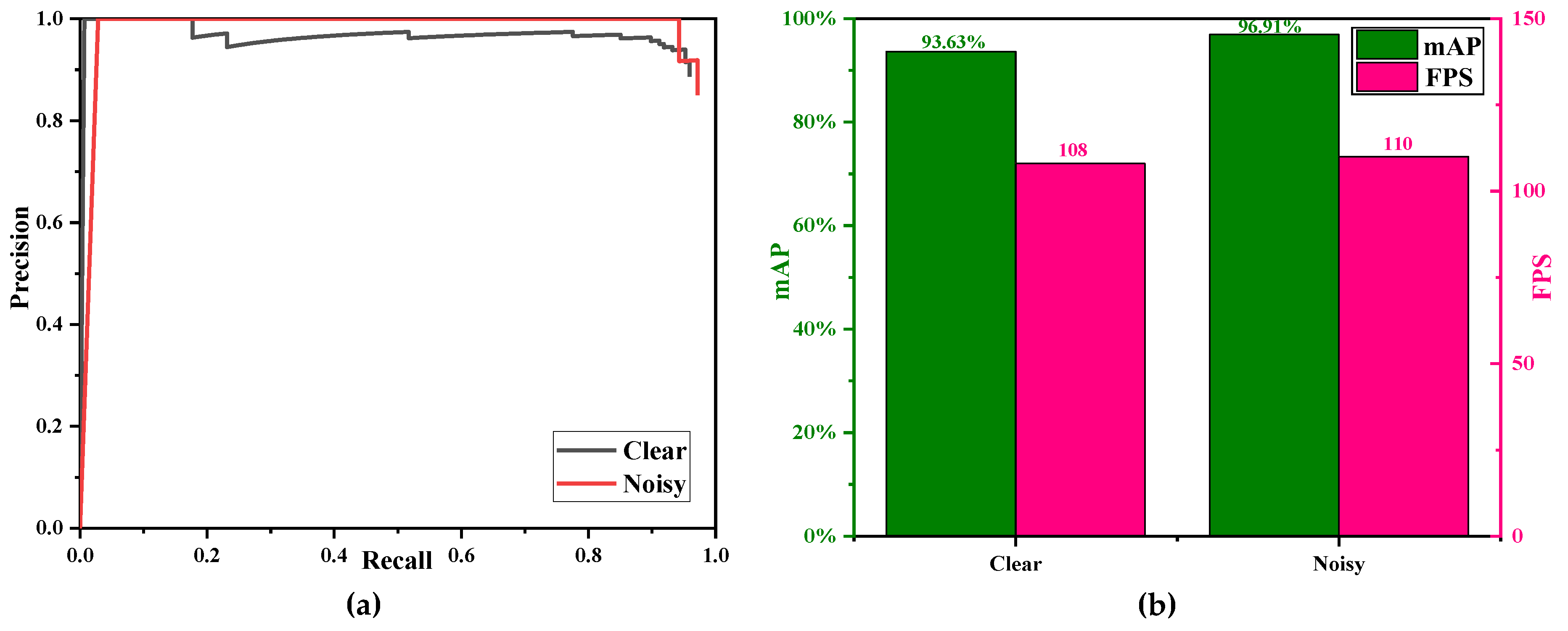
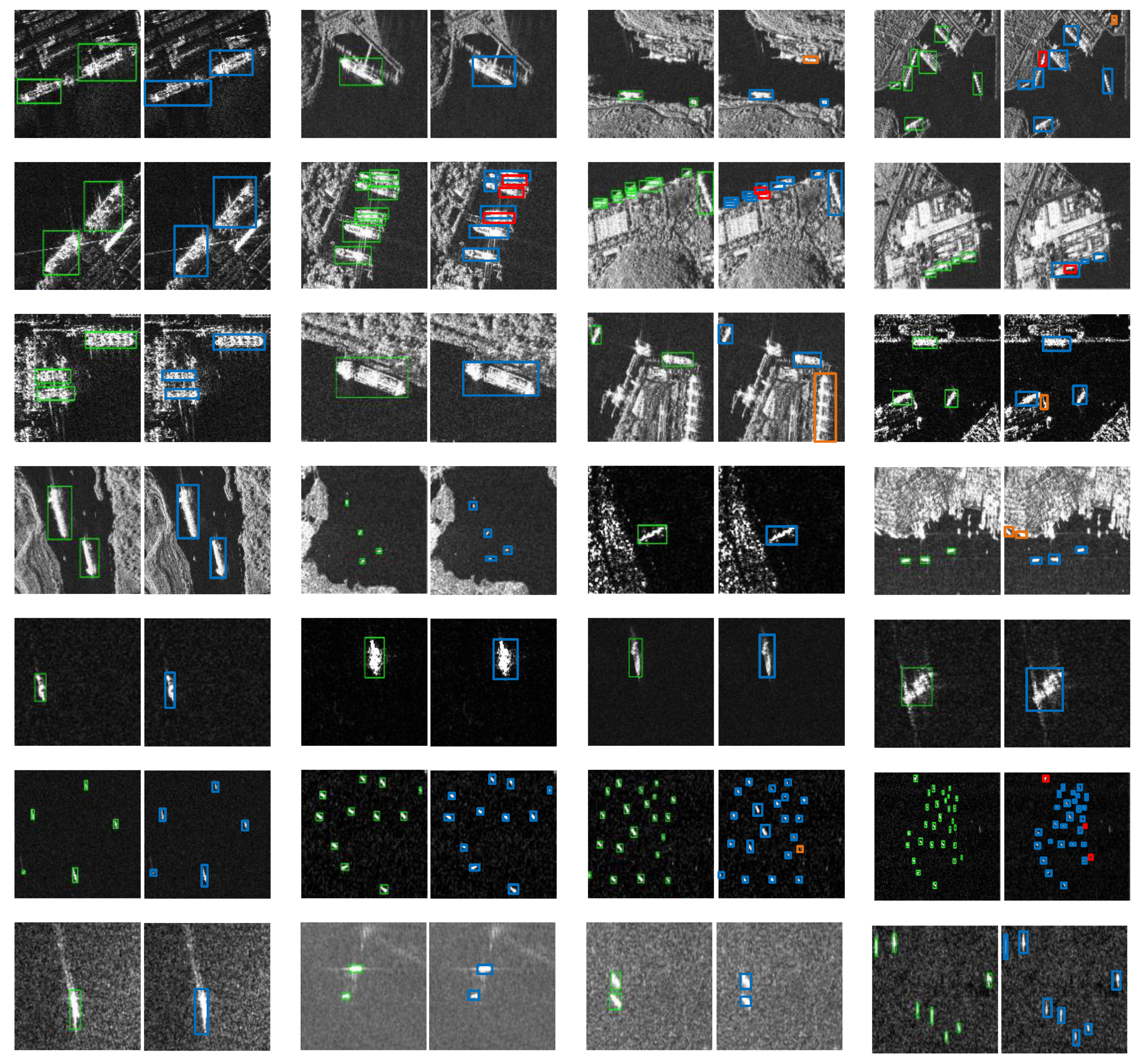
shows the ship detection evaluation indexes of images with severe speckle noise and clear images. Figure 20a shows the precision-recall (P-R) curves and Figure 20b is the bar graph of mAP (accuracy) and FPS (speed). Figure 21 shows the ship detection results of images with severe speckle noise and clear images.

From Table 9, Figure 20 and Figure 21, we can draw the following conclusions:

(1)

The detection accuracy of the nosiy images is superior to that of the clear images (96.91% mAP > 93.63% mAP). This phenomenon seems to be out of line with common sense, because usually, clear images should have higher accuracy than noisy ones. In fact, the possible reasons for this phenomenon are that (1) in the test set of the SSDD dataset (1160 × 10% = 116), the number of moisy images is less than that of clear images (28 of 116 < 88 of 116), which may lead to greater accuracy randomness; (2) noisy images have a single background and contain offshore ships (See Figure 21a) while clear images have more complex backgrounds and contain onshore ships (See Figure 21b), and evidently, it is more difficulty to detect the onshore ships than the offshore ships;

(2)

The detection speed of the clear images is similar to that of the nosiy images, because the size of images is the same.

6.2. Results of Ship Detection on Sentinel-1

In order to verify that our ship detection model has strong migration ability, we carried out actual ship detection on a wide-region large-size Sentinel-1 SAR image with multiple targets and complex backgrounds. We obtained this SAR image from the website of reference [70], and obtained the ground truth information from the Association for Information Systems (AIS) [71,72].

Table 10. Descriptions of the Sentinel-1 SAR image. Az.: Azimuth; Rg.: Range. H: Horizontal; V: Vertical.

Cover Area	Resolution Az. × Rg.	Imaging Mode	Incident Angle	Image Size Pixel × Pixel	Band	Time	Polarization
Zhe Jiang, China	10 m × 10 m	IW 1	34~46°	6333 × 4185	C	8 July 2015	VV, VH

¹ The Interferometric Wide (IW) swath mode is the main acquisition mode over land and satisfies the majority of service requirements [72]. It acquires data with a 250 km swath at 5 m by 20 m spatial resolution (single look) [72]. IW mode captures three sub-swaths using Terrain Observation with Progressive Scans SAR (TOPSAR) [73].

shows the descriptions of the Sentinel-1 SAR image to be detected.

We directly divided the original wide-region large-size SAR image (6333 × 4185) into 900 sub-images on average, with 211 × 140 size for each sub-image, and then resized these 900 sub-images into 160 × 160. Finally, these sub-images were inputted into our high-speed SAR ship detection system to carry out the actual ship detection.

Figure 22 shows the ship detection results of the Sentinel-1 SAR image. From Figure 22, our method can detect almost all ships (marked in blue). There are some false alarm cases on land (marked in yellow), which is due to the high similarity between these land facilities and real ships. Besides, there are some missed detection cases (marked in red), which may be due to the dense distribution or parallel parking of ships, causing certain difficulties for detection. In short, our method has strong migration ability which can be applied in practical SAR ship detection.

Then, we evaluated our model on the Sentinel-1 SAR image.

Table 11. Evaluation indexes of the ship detection results of the Sentinel-1 SAR image.

Precision	Recall	mAP	Time of Preprocessing (s)	Time of Sub-Image (s)	FPS of Sub-Image	Time of Whole Image (s)
91.15%	89.63%	90.36%	54.85 × 10−3	8.92 × 10−3	116	8.09

shows the evaluation indexes of the Sentinel-1 SAR image. Figure 23a shows the precision-recall (P-R) curves and Figure 23b is the bar graph of mAP (accuracy) and FPS (speed).

From Table 11 and Figure 23, our method has high accuracy with 90.36% mAP, which can meet the practical application requirements. The time to divide the wide-region large-size SAR image into small-size sub-images (time of preprocessing) is 54.85 × 10⁻³ s by using Python Imaging Library (PIL), an image preprocessing tool. Additionally, our method takes only 8.92 × 10⁻³ s for one sub-image (160 × 160) similar to the detection time in SSDD dataset (9.03 × 10⁻³ s), and takes only 8.09 s (8.92 × 10⁻³ s × 900 + 54.85 × 10⁻³ s = 8.09 s) to complete the whole wide-region large-size SAR image detection (6333 × 4185). Therefore, our method is of value in practical application from the above detection results.

6.3. Compared with C-CNN

From Figure 4, there are 13 DS-CNNs in our backbone network, which are used to extract ships’ features. To confirm that DS-CNN can really speed up ship detection and sacrifice little accuracy, we replaced these 13 DS-CNNs in Figure 4 with 13 C-CNNs to carry out further research, as is shown in Figure 24.

In addition, in order to ensure the rationality of the study, we arranged the following two groups of experiments under the following same conditions:

(a)

L = 160;

(b)

Pretraining;

(c)

Two concatenations;

(d)

Three scales detection;

(e)

Nine anchor boxes.

In particular, we only compared the detection speed of small-size sub-images in the test set of the SSDD dataset, because the faster detection speed of small-size sub-images will naturally bring about the increase of detection speed of wide-region large-size images.

Table 12. Evaluation indexes of C-CNN and DS-CNN.

Name	Precision	Recall	mAP	Time (ms)	FPS
C-CNN	89.29%	96.15%	94.39%	24.17	41
DS-CNN	87.94%	96.15%	94.13%	9.03	111

shows the evaluation indexes of C-CNN and DS-CNN. Figure 25a shows the precision-recall (P-R) curves and Figure 25b is the bar graph of mAP (accuracy) and FPS (speed).

From Table 12 and Figure 25, we can draw the following conclusions:

(1)

The detection accuracy of DS-CNN is slightly lower than C-CNN (94.13% mAP < 94.39% mAP). This phenomenon shows that using DS-CNN to build a network is feasible and does not decline the detection accuracy too much;

(2)

The detection speed of DS-CNN is 2.7 times than C-CNN (111 FPS > 41 FPS). This phenomenon shows that DS-CNN can indeed improve the detection speed by using D-Conv2D and P-Conv2D to replace C-CNN.

Especially, it is meaningful to increase the detection speed from 41 FPS to 111 FPS for 160 × 160 images. For example, DS-CNN only takes 10.45 s to complete the ship detection task of 1160 SAR images in the SSDD dataset, while C-CNN needs 28.2 s. In general, even millisecond level time saving is meaningful and valuable in the field of image processing. In addition, for the wide-region large-size SAR image (6333 × 4185) in Figure 22, the detection time of DS-CNN is 8.09 s, while that of C-CNN is 21.8 s. From the perspective of image processing, such much time saving is remarkable, which can facilitate subsequent reprocessing (such as ship classification) and improve efficiency of full-link SAR application. Most noteworthy, generally, the size of SAR images acquired from spaceborne SAR satellites is often larger (tens of thousands of pixels × tens of thousands of pixels), so in this case, the advantages of DS-CNN will be better reflected.

We also compared the network sizes of C-CNN and DS-CNN. In the DL field, the number of network parameters, model file size, and weight file size are often used to measure the size of the network. Therefore, we made a comparison from the above three perspectives to illustrate the lightweight nature of our network.

Table 13. Network sizes of C-CNN and DS-CNN.

Method	Number of Parameters	Model File Size (KByte)	Weight File Size (KByte)
C-CNN	28,352,054	334,783	119,986
DS-CNN	3,299,862	38,965	13,159

shows the network sizes of C-CNN and DS-CNN.

From Table 13, the number of network parameters of our proposed DS-CNN is only 3,299,862, which is about one-ninth of the C-CNN’s (28,352,054). Similarly, the model file size and weight file size are nearly one-tenth of the C-CNN’s. Therefore, our network is lighter, leading to higher training efficiency and faster detection speed, which accords with the theoretical analysis before in Section 2.3.

Figure 26 shows the ship detection results of C-CNN and DS-CNN. From Figure 26, both C-CNN and DS-CNN can detect almost all ships successfully, with similar accuracy. In addition, for the second image in Figure 26, DS-CNN generates more missed detection cases (the number of missed detection is (3) than C-CNN (the number of missed detection is (1). One possible reason is that DS-CNN does not adequately extract features from the inshore ships.

Therefore, our method is effective and brilliant. Despite of the slight sacrifice of accuracy for the inshore ships, the detection speed has got largely improved.

6.4. Compared with Other Object Detectors

In order to prove that our method can authentically achieve high-speed ship detection, we also compared the performance with other object detectors, such as Faster R-CNN, RetinaNet, SSD, YOLOv1, YOLOv2, YOLOv2-tiny, YOLOv3, and YOLOv3-tiny. Here, YOLOv2-tiny and YOLOv3-tiny are two lightweight networks that improve YOLOv2 and YOLOv3 respectively, proposed by Redmon et al. [31,32]. Moreover, in order to ensure the rationality of experiments, these other object detectors are implemented on the same platform, and the training mechanism is basically consistent.

Especially, the detection speed of the traditional feature extraction methods is quite slow, whose detection time reaches several seconds or more per image, while the modern DL methods only need tens or hundreds of milliseconds per image. Therefore, we ignored the comparison with the traditional feature extraction methods.

Table 14. Evaluation indexes of different object detectors.

Method	Precision	Recall	mAP	Time (ms)	FPS
Faster R-CNN	81.15%	85.16%	82.66%	327.48	3
RetinaNet	93.12%	96.70%	95.68%	314.43	3
SSD	85.15%	94.51%	92.67%	48.86	20
YOLOv3	93.62%	96.70%	95.34%	22.30	45
YOLOv3-tiny	77.58%	70.33%	64.64%	10.25	98
YOLOv2	84.92%	92.86%	90.09%	19.01	53
YOLOv2-tiny	73.73%	47.80%	44.40%	9.43	107
YOLOv1	84.53%	84.07%	81.24%	21.95	46
Our method	87.94%	96.15%	94.13%	9.03	111

shows the evaluation indexes of different object detectors. Figure 27 shows the precision-recall (P-R) curves and Figure 28 is the bar graph of mAP (accuracy) and FPS (speed).

From Table 14 and Figure 27 and Figure 28, we can draw the following conclusions:

(1)

The detection accuracy of our method is slightly lower than RetinaNet (94.13% mAP < 95.68% mAP). However, our detection speed is almost 37 times faster than RetinaNet. Therefore, it is of far-reaching significance that a little sacrifice of accuracy brings about a multiplier increase in speed;

(2)

The detection accuracy of our method is also slightly lower than YOLOv3 (94.13% mAP < 95.34% mAP). However, our detection speed is 2.47 times faster than YOLOv3. Therefore, our approach is still excellent because we traded 2.1% accuracy for a 147% speed increase;

(3)

The detection accuracy and speed of our method are all superior to Faster R-CNN, SSD, YOLOv1, YOLOv2, and YOLOv3-tiny;

(4)

The detection speed of our method is slightly faster than YOLOv2-tiny (111 FPS > 107 FPS). However, the detection accuracy of YOLOv2-tiny is too poor to meet the actual detection requirements at all (44.40% mAP), which is far lower than that of our method (94.13% mAP);

(5)

The detection speed of our method is superior to all other methods (9.03 ms per image and 111 FPS);

(6)

Our method has not only the fastest detection speed but also satisfactory accuracy (Both mAP and FPS are high in Figure 28), while other methods cannot maintain a good balance between accuracy and speed.

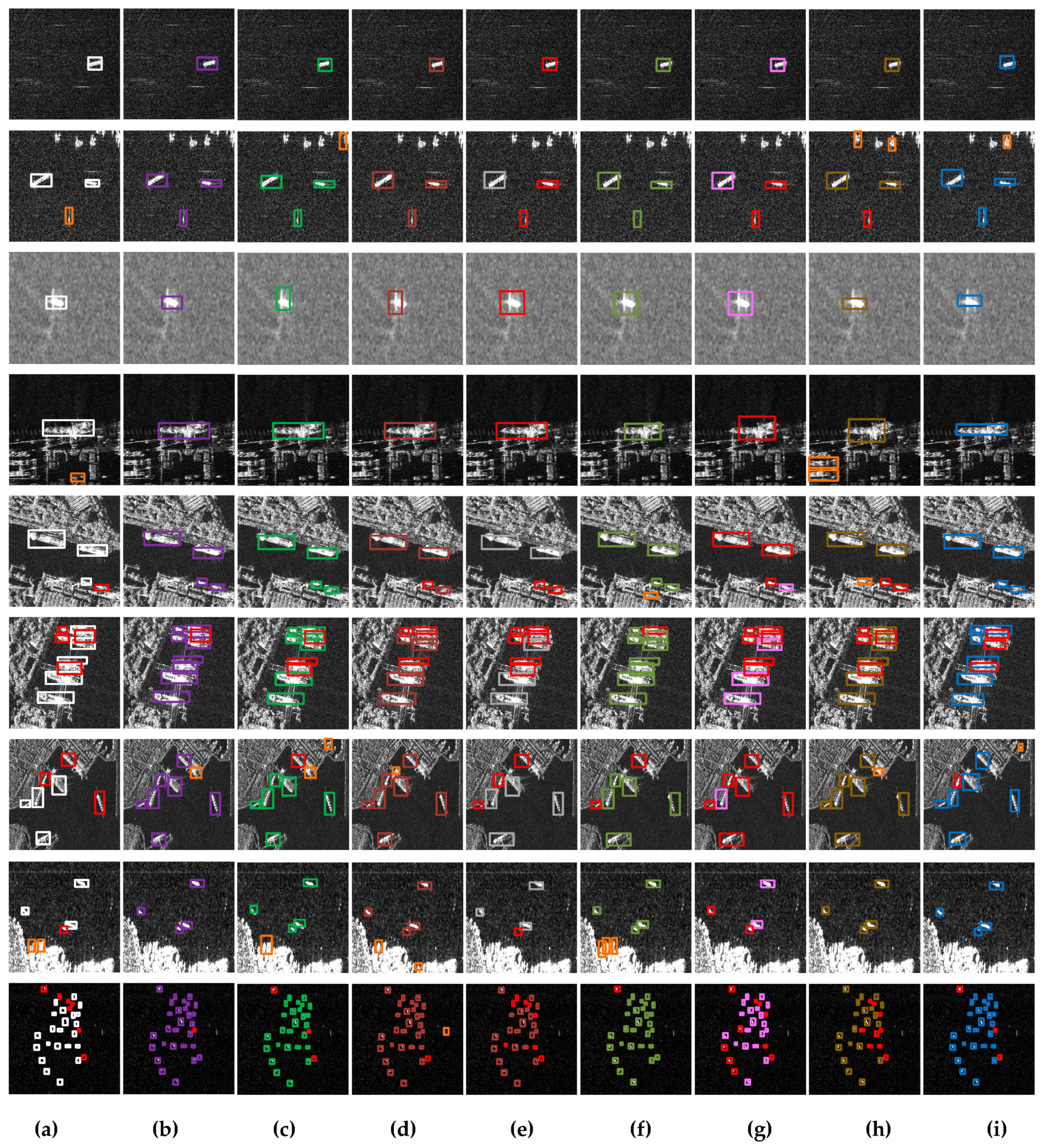
Figure 29 shows the ship detection results of some sample images of different object detectors. From Figure 29, we can draw the following conclusions:

(1)

All methods can successfully detect ships in simple sample images, except YOLOv3-tiny and YOLOv2-tiny;

(2)

YOLOv3-tiny and YOLOv2-tiny generate more missed detection cases;

(3)

RetinaNet and YOLOv2 have a better detection performance for small ships with dense distribution, with only one missed detection case;

(4)

Compared with RetinaNet and YOLOv2, YOLOv3 have similar detection performance for small ships with dense distribution, with only one missed detection case and only one false alarm case;

(5)

Compared with all other methods, from a subjective point of view in Figure 29, our method has obtained satisfactory ship detection results, although not the best.

We also compared the network sizes of other object detectors.

Table 15. Network sizes of different object detectors.

Method	Number of Parameters	Model File Size (KByte)	Weight File Size (KByte)
YOLOv1	272,746,867	2,308,877	770,814
YOLOv3	61,576,342	722,131	241,082
YOLOv2	50,578,686	592,777	197,668
RetinaNet	36,382,957	426,195	142,573
Faster R-CNN	28,342,195	310,112	111,144
SSD	23,745,908	278,550	92,904
YOLOv2-tiny	15,770,510	184,858	61,646
YOLOv3-tiny	8,676,244	101,799	33,990
Our method	3,299,862	38,965	13,159

shows the network sizes of different object detectors. From Table 15, our model has the fewest network parameters only 3,299,862, while the numbers of network parameters of other methods are several or even tens of times than that of our method. Moreover, the model file size and the weight file size are also minimal compared with other methods. Therefore, our network is lighter, leading to higher training efficiency and faster detection speed, which also accords with the theoretical analysis before in Section 2.3.

In summary, by comparing the actual network size, it further more forcefully indicated that our method can achieve high-speed SAR ship detection.

6.5. Compared with References

We also compared our methods with some previous open studies which use the same SSDD dataset. To be clear, here, we replaced NVIDIA RTX2080Ti GPU with NVIDIA GTX1080 GPU to keep the hardware environment basically the same as previous other open studies (References [10,21,35,59,60,61,62] used NVIDIA GTX1080 GPU.). For different performances of different types of GPUs, we have to make such a replacement in order to consider the rationality of the comparison experiment.

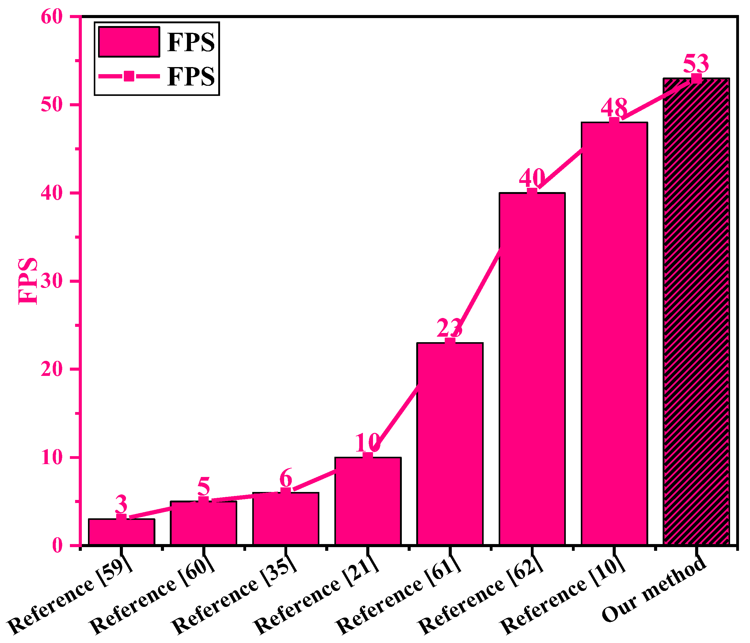
Figure 30 shows the contrast results of ship detection speed (FPS, Frames Per Second) between our method and previous other open studies.

From Figure 30, the ship detection speed of our method is 53 FPS under the NVIDIA GTX1080 GPU, which is the half of that under the NVIDIA RTX2080Ti GPU (111 FPS introduced before). This phenomenon is in line with common sense, because the performance of RTX2080Ti GPU is superior to that of GTX1080 GPU. In Figure 30, our method has the fastest detection speed compared with the other references under the similar hardware environment with NVIDIA GTX1080 GPU. Most noteworthy, the detection speed of reference [10] is 48 FPS, which is close to that of the method in this paper (53 FPS). However, the accuracy of reference [10] is lower than ours (Reference [10]: 90.16% mAP; Ours: 94.13% mAP).

Therefore, our method can reliably realize high-speed SAR ship detection. In addition, due to the lacking of specific type GPUs, we cannot make full comparisons between our method and the remaining studies using the same SSDD dataset.

7. Conclusions

Aiming at the problem that the detection speed of SAR ship is often neglected at present, in this paper, a brand-new light-weight network was established with fewer network parameters by mainly using DS-CNN to achieve high-speed SAR ship detection. DS-CNN is composed of D-Conv2D and P-Conv2D, which substitute for the C-CNN, by which the number of network parameters get greatly decreased. Consequently, the detection speed gets dramatically improved. In addition, multi-scale detection mechanism, concatenation mechanism and anchor box mechanism are integrated into our network to improve the detection accuracy. We verified the correctness and effectiveness of the proposed method on an open SSDD dataset. The experimental results indicated that our method has the faster ship detection speed than other object detectors, under the same hardware platform, with 9.03 ms per image and 111 FPS, meanwhile the detection accuracy is only lightly sacrificed compared with the state-of-art object detectors. Besides, we also discussed the reasons why the proposed method can achieve high-speed ship detection via theoretical complexity analysis and calculation of network size. Our method can achieve high-speed and accurate ship detection simultaneously (111 FPS and 94.13% mAP) compared with other methods, which has great application value in real-time maritime disaster rescue and emergency military planning.

References

1. Born, G.H.; Dunne, J.A.; Lame, D.B. Seasat mission overview. Science 1979, 204, 1405–1406. [Google Scholar] [CrossRef] [PubMed]
2. Petit, M.; Stretta, J.M.; Farrugio, H.; Wadsworth, A. Synthetic aperture radar imaging of sea surface life and fishing activities. IEEE Trans. Geosci. Remote Sens. 1992, 30, 1085–1089. [Google Scholar] [CrossRef] [Green Version]
3. Cerutti-Maori, D.; Klare, J.; Brenner, A.R.; Ender, J.H.G. Wide-area traffic monitoring with the SAR/GMTI system pamir. IEEE Trans. Geosci. Remote Sens. 2008, 46, 3019–3030. [Google Scholar] [CrossRef]
4. Dierking, W.; Busche, T. Sea ice monitoring by L-band SAR: An assessment based on literature and comparisons of JERS-1 and ERS-1 imagery. IEEE Trans. Geosci. Remote Sens. 2006, 44, 957–970. [Google Scholar] [CrossRef]
5. Solberg, A.H.S.; Storvik, G.; Solberg, R.; Volden, E. Automatic detection of oil spills in ERS SAR images. IEEE Trans. Geosci. Remote Sens. 1999, 37, 1916–1924. [Google Scholar] [CrossRef] [Green Version]
6. Brusch, S.; Lehner, S.; Fritz, T.; Soccorsi, M.; Soloviev, A.; Van Schie, B. Ship surveillance with TerraSAR-X. IEEE Trans. Geosci. Remote Sens. 2011, 49, 1092–1103. [Google Scholar] [CrossRef]
7. Zhao, Z.; Ji, K.; Xing, X.; Zou, H.; Zhou, S. Ship surveillance by integration of space-borne SAR and AIS—Review of current research. J. Navig. 2014, 67, 177–189. [Google Scholar] [CrossRef]
8. Vachon, P.W.; Thomas, S.J.; Cranton, J.; Edel, H.R.; Henschel, M.D. Validation of ship detection by the RADARSAT synthetic aperture radar and the ocean monitoring workstation. Can. J. Remote Sens. 2000, 26, 200–212. [Google Scholar] [CrossRef]
9. Wackerman, C.C.; Friedman, K.S.; Pichel, W.G.; Clemente-Colón, P.; Li, X. Automatic detection of ships in RADARSAT-1 SAR imagery. Can. J. Remote Sens. 2001, 27, 568–577. [Google Scholar] [CrossRef]
10. Zhang, T.; Zhang, X. High-Speed Ship Detection in SAR Images Based on a Grid Convolutional Neural Network. Remote Sens. 2019, 11, 1206. [Google Scholar] [CrossRef]
11. Zhou, D.; Zeng, L.; Zhang, K. A novel SAR target detection algorithm via multi-scale SIFT features. J. Northwest. Polytech. Univ. 2015, 33, 867–873. [Google Scholar]
12. Schwegmann, C.P.; Kleynhans, W.; Salmon, B.P. Ship detection in South African oceans using SAR, CFAR and a Haar-like feature classifier. In Proceedings of the 2014 IEEE Geoscience and Remote Sensing Symposium, Quebec City, QC, Canada, 13–18 July 2014. [Google Scholar]
13. Xu, F.; Liu, J.H. Ship detection and extraction using visual saliency and bar graph of oriented gradient. Optoelectron. Lett. 2016, 12, 473–477. [Google Scholar] [CrossRef]
14. Raj, N.; Sethunadh, R.; Aparna, P.R. Object detection in SAR image based on bandlet transform. J. Vis. Commun. Image Represent. 2016, 40, 376–383. [Google Scholar] [CrossRef]
15. Xu, X.; Zheng, R.; Chen, G.; Blasch, E. Performance analysis of order statistic constant false alarm rate (CFAR) detectors in generalized Rayleigh environment. In Proceedings of SPIE; The International Society for Optical Engineering: Bellingham, WA, USA, 2007. [Google Scholar]
16. Watts, S. Radar detection prediction in sea clutter using the compound k-distribution model. IEEE Proc. Commun. Radar Signal Process. 1985, 132, 613. [Google Scholar] [CrossRef]
17. Anastassopoulos, V.; Lampropoulos, G.A. Optimal CFAR detection in weibull clutter. IEEE Trans. Aerosp. Electron. Syst. 1995, 31, 52–64. [Google Scholar] [CrossRef]
18. Wang, C.; Bi, F.; Chen, L.; Chen, J. A novel threshold template algorithm for ship detection in high-resolution SAR images. In Proceedings of the 2016 IEEE Geoscience & Remote Sensing Symposium, Beijing, China, 10–15 July 2016. [Google Scholar]
19. Zhu, J.; Qiu, X.; Pan, Z.; Zhang, Y.; Lei, B. Projection shape template-based ship target recognition in TerraSAR-X images. IEEE Geosci. Remote Sens. Lett. 2017, 14, 222–226. [Google Scholar] [CrossRef]
20. Lecun, Y.; Bengio, Y.; Hinton, G. Deep learning. Nature 2015, 521, 436. [Google Scholar] [CrossRef]
21. Gui, Y.; Li, X.; Xue, L. A Multilayer Fusion Light-Head Detector for SAR Ship Detection. Sensors 2019, 19, 1124. [Google Scholar] [CrossRef]
22. Girshick, R.; Donahue, J.; Darrell, T.; Malik, J. Rich Feature Hierarchies for Accurate Object Detection and Semantic Segmentation. In Proceedings of the IEEE Conference on Computer Vision and Pattern Recognition, Columbus, OH, USA, 23–28 June 2014; pp. 580–587. [Google Scholar]
23. Uijlings, J.R.R.; Sande, K.E.A.V.D.; Gevers, T.; Smeulders, A.W.M. Selective search for object recognition. Int. J. Comput. Vis. 2013, 104, 154–171. [Google Scholar] [CrossRef]
24. Adankon, M.M.; Cheriet, M. Support vector machine. Comput. Sci. 2002, 1, 1–28. [Google Scholar]
25. Everingham, M.; Eslami, S.A.; Van Gool, L.; Williams, C.K.; Winn, J.; Zisserman, A. The Pascal Visual Object Classes Challenge: A Retrospective. Int. J. Comput. Vis. 2015, 111, 98–136. [Google Scholar] [CrossRef]
26. Girshick, R. Fast R-CNN. In Proceedings of the 2015 IEEE International Conference on Computer Vision (ICCV), Santiago, Chile, 7–13 December 2015; pp. 1440–1448. [Google Scholar]
27. He, K.; Zhang, X.; Ren, S.; Sun, J. Spatial pyramid pooling in deep convolutional networks for visual recognition. IEEE Trans. Pattern Anal. Mach. Intell. 2014, 37, 1904–1916. [Google Scholar] [CrossRef] [PubMed]
28. Ren, S.; He, K.; Girshick, R.; Sun, J. Faster R-CNN: Towards Real-Time Object Detection with Region Proposal Networks. IEEE Trans. Pattern Anal. Mach. Intell. 2017, 39, 1137–1149. [Google Scholar] [CrossRef] [PubMed] [Green Version]
29. Wang, Z.; Liu, J. A review of object detection based on convolutional neural network. In Proceedings of the IEEE 2017 36th Chinese Control Conference (CCC), Dalian, China, 26–28 July 2017. [Google Scholar]
30. Redmon, J.; Divvala, S.; Girshick, R.; Farhadi, A. You Only Look Once: Unified, Real-Time Object Detection. In Proceedings of the 2016 IEEE Conference on Computer Vision and Pattern Recognition (CVPR), Las Vegas, NV, USA, 27–30 June 2016. [Google Scholar]
31. Redmon, J.; Farhadi, A. YOLO9000: Better, Faster, Stronger. In Proceedings of the 2017 IEEE Conference on Computer Vision and Pattern Recognition (CVPR), Honolulu, HI, USA, 21–26 July 2017; pp. 6517–6525. [Google Scholar]
32. Redmon, J.; Farhadi, A. YOLOv3: An incremental improvement. arXiv 2018, arXiv:1804.02767. [Google Scholar]
33. Liu, W.; Anguelov, D.; Erhan, D.; Szegedy, C.; Reed, S.E.; Fu, C.-Y.; Berg, A.C. SSD: Single Shot MultiBox Detector. In Proceedings of the European Conference on Computer Vision (ECCV), Amsterdam, The Netherlands, 8–16 October 2016; pp. 21–37. [Google Scholar]
34. Lin, T.Y.; Goyal, P.; Girshick, R.; He, K.; Dollár, P. Focal loss for dense object detection. IEEE Trans. Pattern Anal. Mach. Intell. 2017, 2999–3007. [Google Scholar] [CrossRef]
35. Li, J.; Qu, C.; Shao, J. Ship detection in SAR images based on an improved faster R-CNN. In Proceedings of the 2017 SAR in Big Data Era: Models, Methods and Applications (BIGSARDATA), Beijing, China, 13–14 November 2017. [Google Scholar]
36. Lecun, Y.; Bottou, L.; Bengio, Y.; Haffner, P. Gradient-based learning applied to document recognition. Proc. IEEE 1998, 86, 2278–2324. [Google Scholar] [CrossRef] [Green Version]
37. Zhang, Q.Q.; Liu, Y.; Pan, J.L.; Yan, Y.H. Continuous speech recognition by convolutional neural networks. Chin. J. Eng. 2015, 5, 85–95. [Google Scholar]
38. Krizhevsky, A.; Sutskever, I.; Hinton, G. ImageNet Classification with Deep Convolutional Neural Networks; NIPS (Vol. 25); Curran Associates Inc.: New York, NY, USA, 2012. [Google Scholar]
39. Li, H. Deep learning for natural language processing: Advantages and challenges. Natl. Sci. Rev. 2018, 5, 24–26. [Google Scholar] [CrossRef]
40. Russakovsky, O.; Deng, J.; Su, H.; Krause, J.; Satheesh, S.; Ma, S.; Huang, Z.; Karpathy, A. ImageNet large scale visual recognition challenge. Int. J. Comput. Vis. 2015, 115, 211–252. [Google Scholar] [CrossRef]
41. Hubel, D.H.; Wiesel, T.N. Receptive fields of single neurones in the cat’s striate cortex. J. Physiol. 1959, 148, 574. [Google Scholar] [CrossRef]
42. Simonyan, K.; Zisserman, A. Very deep convolutional networks for large-scale image recognition. arXiv 2014, arXiv:1409.1556. [Google Scholar]
43. Szegedy, C.; Liu, W.; Jia, Y.; Sermanet, P.; Reed, S.; Anguelov, D.; Erhan, D.; Vanhoucke, V.; Rabinovich, A. Going Deeper with Convolutions. In Proceedings of the 2015 IEEE Conference on Computer Vision and Pattern Recognition (CVPR), Boston, MA, USA, 7–12 June 2015. [Google Scholar]
44. Howard, A.G.; Zhu, M.; Chen, B.; Kalenichenko, D.; Wang, W.; Weyand, T.; Andreetto, M.; Adam, H. MobileNets: Efficient Convolutional Neural Networks for Mobile Vision Applications. arXiv 2017, arXiv:1704.04861. [Google Scholar]
45. Sifre, L. Rigid-Motion Scattering for Image Classification. Ph.D. Thesis, Ecole Polytechnique, Palaiseau, France, 2014. [Google Scholar]
46. Chollet, F. Xception: Deep learning with depthwise separable convolutions. arXiv 2016, arXiv:1610.02357v2. [Google Scholar]
47. Huang, G.; Liu, Z.; Laurens, V.D.M.; Weinberger, K.Q. Densely connected convolutional networks. arXiv 2016, arXiv:1608.06993. [Google Scholar]
48. Ioffe, S.; Szegedy, C. Batch Normalization: Accelerating Deep Network Training by Reducing Internal Covariate Shift. In Proceedings of the International Conference on International Conference on Machine Learning, Lille, France, 6–11 July 2015. [Google Scholar]
49. Xu, B.; Wang, N.; Chen, T.; Li, M. Empirical evaluation of rectified activations in convolutional network. arXiv 2018, arXiv:1505.00853. [Google Scholar]
50. Hosang, J.; Benenson, R.; Schiele, B. Learning Non-maximum Suppression. In Proceedings of the 2017 IEEE Conference on Computer Vision and Pattern Recognition, Honolulu, HI, USA, 21–26 July 2017; pp. 6469–6477. [Google Scholar]
51. Pycharm. Available online: http://www.jetbrains.com/pycharm/ (accessed on 6 September 2019).
52. Manaswi, N.K. Understanding and Working with Keras. In Deep Learning with Applications Using Python; Apress: Berkeley, CA, USA, 2018. [Google Scholar]
53. Abadi, M.; Agarwal, A.; Barham, P.; Brevdo, E.; Chen, Z.; Citro, C.; Corrado, G.S.; Davis, A.; Dean, J.; Devin, M.; et al. Tensorflow: Large-scale Machine Learning on Heterogeneous Systems. 2015. Available online: https://arxiv.org/abs/1603.04467; https://www.tensorflow.org (accessed on 24 October 2019).
54. LabelImg. Available online: https://github.com/tzutalin/labelImg. (accessed on 6 September 2019).
55. Cui, Z.; Li, Q.; Cao, Z.; Liu, N. Dense Attention Pyramid Networks for Multi-Scale Ship Detection in SAR Images. IEEE Trans. Geosci. Remote Sens. 2019. [Google Scholar] [CrossRef]
56. Jiao, J.; Yue, Z.; Hao, S.; Xue, Y.; Xun, G.; Wen, H.; Fu, K.; Sun, X. A densely connected end-to-end neural network for multiscale and multiscene sar ship detection. IEEE Access 2018, 6, 20881–20892. [Google Scholar] [CrossRef]
57. Liu, N.; Cao, Z.; Cui, Z.; Pi, Y.; Dang, S. Multi-Scale Proposal Generation for Ship Detection in SAR Images. Remote Sens. 2019, 11, 526. [Google Scholar] [CrossRef]
58. Chang, Y.-L.; Anagaw, A.; Chang, L.; Wang, Y.C.; Hsiao, C.-Y.; Lee, W.-H. Ship Detection Based on YOLOv2 for SAR Imagery. Remote Sens. 2019, 11, 786. [Google Scholar] [CrossRef]
59. Li, J.; Qu, C.; Peng, S.; Jiang, Y. Ship Detection in SAR images Based on Generative Adversarial Network and Online Hard Examples Mining. J. Electron. Inf. Technol. 2019, 41, 143–149. [Google Scholar]
60. Li, J.; Qu, C.; Peng, S.; Deng, B. Ship detection in SAR images based on convolutional neural network. Syst. Eng. Electron. 2018, 40, 1953–1959. [Google Scholar]
61. Wang, Y.; Chao, W.; Hong, Z. Combining a single shot multibox detector with transfer learning for ship detection using sentinel-1 SAR images. Remote Sens. Lett. 2018, 9, 780–788. [Google Scholar] [CrossRef]
62. Wang, J.; Lu, C.; Jiang, W. Simultaneous Ship Detection and Orientation Estimation in SAR Images Based on Attention Module and Angle Regression. Sensors 2018, 18, 2851. [Google Scholar] [CrossRef] [PubMed]
63. Chen, C.; He, C.; Hu, C.; Pei, H.; Jiao, L. A Deep Neural Network Based on an Attention Mechanism for SAR Ship Detection in Multiscale and Complex Scenarios. IEEE Access 2019, 7, 104848–104863. [Google Scholar] [CrossRef]
64. Kingma, D.; Ba, J. Adam: A Method for Stochastic Optimization. arXiv 2014, arXiv:1412.6980. [Google Scholar]
65. Hinton, G.E.; Srivastava, N.; Krizhevsky, A.; Sutskever, I.; Salakhutdinov, R.R. Improving neural networks by preventing co-adaptation of feature detectors. arXiv 2012, arXiv:1207.0580. [Google Scholar]
66. Yuan, Y.; Rosasco, L.; Caponnetto, A. On early stopping in gradient descent learning. Constr. Approx. 2007, 26, 289–315. [Google Scholar]
67. He, K.; Girshick, R.; Dollár, P. Rethinking ImageNet pre-training. arXiv 2018, arXiv:1811.08883. [Google Scholar]
68. Deng, Z.; Sun, H.; Zhou, S.; Zhao, J. Learning Deep Ship Detector in SAR Images from Scratch. IEEE Trans. Geosci. Remote Sens. 2019, 57, 4021–4039. [Google Scholar] [CrossRef]
69. Zeiler, M.D.; Fergus, R. Visualizing and Understanding Convolutional Networks. arXiv 2013, arXiv:1311.2901v3. [Google Scholar]
70. OpenSAR. Available online: http://opensar.sjtu.edu.cn/ (accessed on 6 September 2019).
71. Huang, L.; Liu, B.; Li, B.; Guo, W.; Yu, W. OpenSARShip: A dataset dedicated to sentinel-1 ship interpretation. IEEE J. Sel. Top. Appl. Earth Obs. Remote Sens. 2017, 11, 195–208. [Google Scholar] [CrossRef]
72. Copernicus Open Access Hub. Available online: https://scihub.copernicus.eu (accessed on 6 September 2019).
73. De Zan, F.; Guarnieri, A.M. TOPSAR: Terrain observation by progressive scans. IEEE Trans. Geosci. Remote Sens. 2006, 44, 2352–2360. [Google Scholar] [CrossRef]
Figure 1. Convolutional neural network. (a) Conventional convolution neural network (C-CNN); (b) depthwise separable convolution neural network (DS-CNN).
Remotesensing 11 02483 g001
Figure 2. Detailed internal operation flow of a DS-CNN. (a) Depthwise convolution (D-Conv2D); (b) pointwise convolution (P-Conv2D).
Remotesensing 11 02483 g002
Figure 3. Computational complexity. (a) C-CNN; (b) DS-CNN.
Remotesensing 11 02483 g003
Figure 4. Network Architecture.
Remotesensing 11 02483 g004
Figure 5. Internal implementation. (a) C-CNN; (b) DS-CNN.
Remotesensing 11 02483 g005
Figure 6. Multi-scale detection mechanism.
Remotesensing 11 02483 g006
Figure 7. Concatenation mechanism.
Remotesensing 11 02483 g007
Figure 8. Detection process of high-speed SAR ship detection system. (a) Original images; (b) resize images; (c) divide images; (d) locate ships’ center; (e) generate bounding boxes; (f) non-maximum suppression; (g) detection results.
Remotesensing 11 02483 g008
Figure 9. Anchor box. (a) An original SAR image with densely distributed small ships (Ground truth is marked in green.); (b) diagram of anchor box mechanism. (c) cluster results of SSDD. (The x axis is the width of ground truth and y axis is the height of ground truth.).
Remotesensing 11 02483 g009
Figure 10. Loss curves of the training set and the validation set.
Remotesensing 11 02483 g010
Figure 11. Research on image size. (a) P-R curves; (b) bar graph of mAP (accuracy) and FPS (speed).
Remotesensing 11 02483 g011
Figure 12. Research on pretraining. (a) P-R curves; (b) bar graph of mAP (accuracy) and FPS (speed).
Remotesensing 11 02483 g012
Figure 13. Research on multi-scale detection mechanism. (a) P-R curves; (b) bar graph of mAP (accuracy) and FPS (speed).
Remotesensing 11 02483 g013
Figure 14. Research on concatenation mechanism. (a) P-R curves; (b) bar graph of mAP (accuracy) and FPS (speed).
Remotesensing 11 02483 g014
Figure 15. Research on anchor box mechanism. (a) P-R curves; (b) bar graph of mAP (accuracy) and FPS (speed).
Remotesensing 11 02483 g015
Figure 16. Ship detection result of an image with densely distributed small ships. (a) Ground truth; (b) 3 anchor boxes; (c) 6 anchor boxes; (d) 9 anchor boxes. (Ground truth is marked in green, missed detection is marked in red, and false alarm is marked in yellow.).
Remotesensing 11 02483 g016
Figure 17. Visualization of feature maps. (a) An original image; (b) output of the 1st layer; (c) output of backbone network; (d) output of detection network-1; (e) output of detection network-2; (f) output of detection network-3.
Remotesensing 11 02483 g017
Figure 18. SAR ship detection results. (Ground truth is marked in green, missed detection is marked in red, and false alarm is marked in yellow).
Remotesensing 11 02483 g018
Figure 19. Results of the test set of SSDD. (a) P-R curves; (b) bar graph of mAP (accuracy) and FPS (speed).
Remotesensing 11 02483 g019
Figure 20. Results of images of with severe speckle noise and clear images. (a) P-R curves; (b) bar graph of mAP (accuracy) and FPS (speed).
Remotesensing 11 02483 g020
Figure 21. SAR ship detection results of images of with severe speckle noise and clear images. (Ground truth is marked in green, missed detection is marked in red, and false alarm is marked in yellow).
Remotesensing 11 02483 g021
Figure 22. Ship detection results of the Sentinel-1 SAR image. (Detection results are marked in blue, missed detection is marked in red, and false alarm is marked in yellow).
Remotesensing 11 02483 g022
Figure 23. Results of the Sentinel-1 image. (a) P-R curves; (b) bar graph of mAP (accuracy) and FPS (speed).
Remotesensing 11 02483 g023
Figure 24. Replace DS-CNN in Figure 4 with C-CNN.
Remotesensing 11 02483 g024
Figure 25. Results of C-CNN and DS-CNN. (a) P-R curves; (b) bar graph of mAP (accuracy) and FPS (speed).
Remotesensing 11 02483 g025
Figure 26. Ship detection results of C-CNN and DS-CNN (a) Ground truth; (b) C-CNN; (c) DS-CNN. (Ground truth is marked in green, missed detection is marked in red, and false alarm is marked in yellow.).
Remotesensing 11 02483 g026
Figure 27. P-R curves of different object detectors.
Remotesensing 11 02483 g027
Figure 28. Bar graph of mAP (accuracy) and FPS (speed) of different object detectors.
Remotesensing 11 02483 g028
Figure 29. SAR ship detection results of different object detectors. (a) Faster R-CNN; (b) RetinaNet; (c) SSD; (d) YOLOv3; (e) YOLOv3-tiny; (f) YOLOv2; (g) YOLOv2-tiny; (h) YOLOv1; (i) Our method. (Missed detection is marked in red, and false alarm is marked in yellow).
Remotesensing 11 02483 g029
Figure 30. Detection speed comparison between our method and references under the similar hardware environment with NVIDIA GTX1080 GPU.
Remotesensing 11 02483 g030