Antarctic Supraglacial Lake Detection Using Landsat 8 and Sentinel-2 Imagery: Towards Continental Generation of Lake Volumes

 , ,
, ,
Abstract
1. Introduction
2. Data and Methods
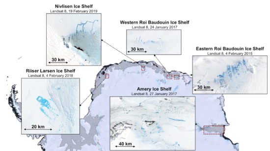
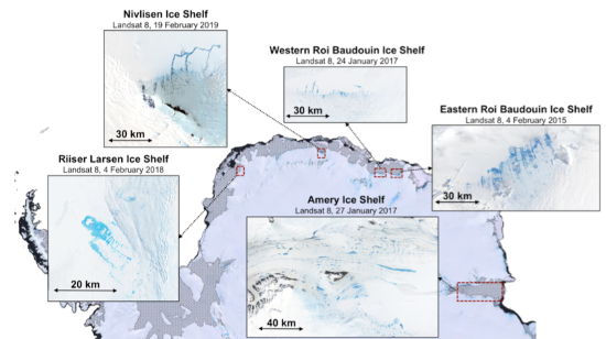
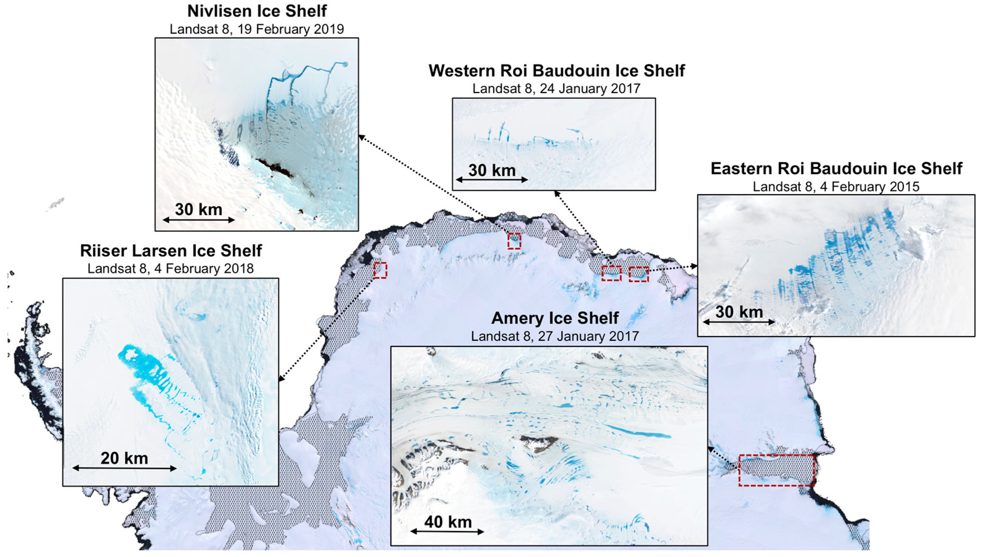
2.1. Study Area
2.2. Image Data Collection and Preprocessing
2.3. Lake Area Delineation
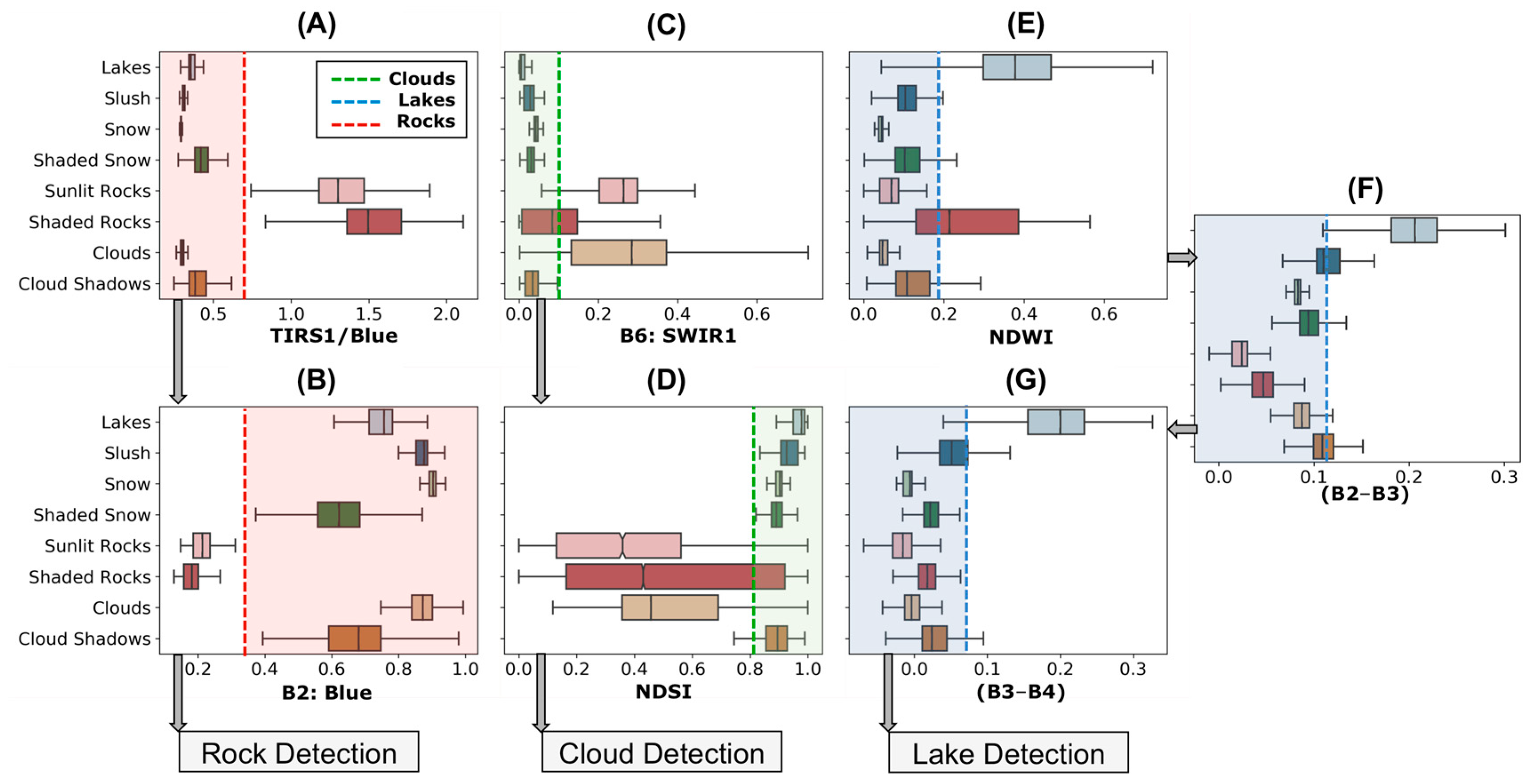
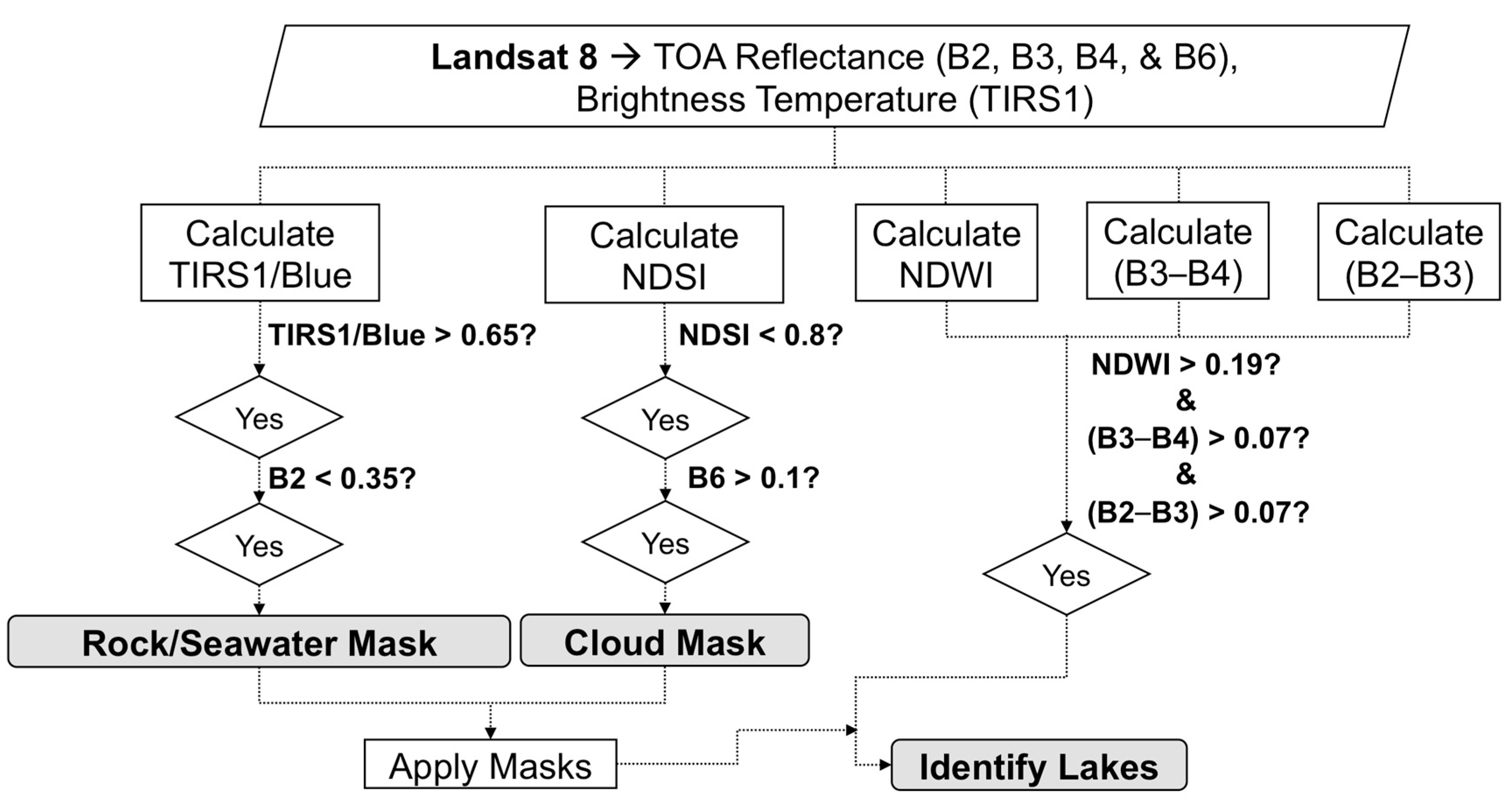
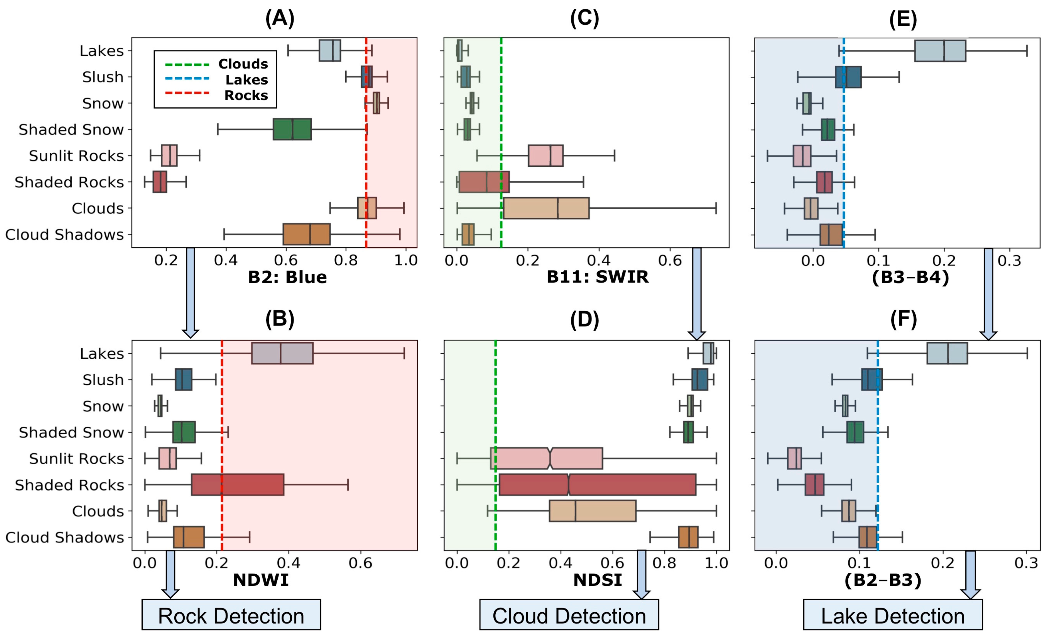
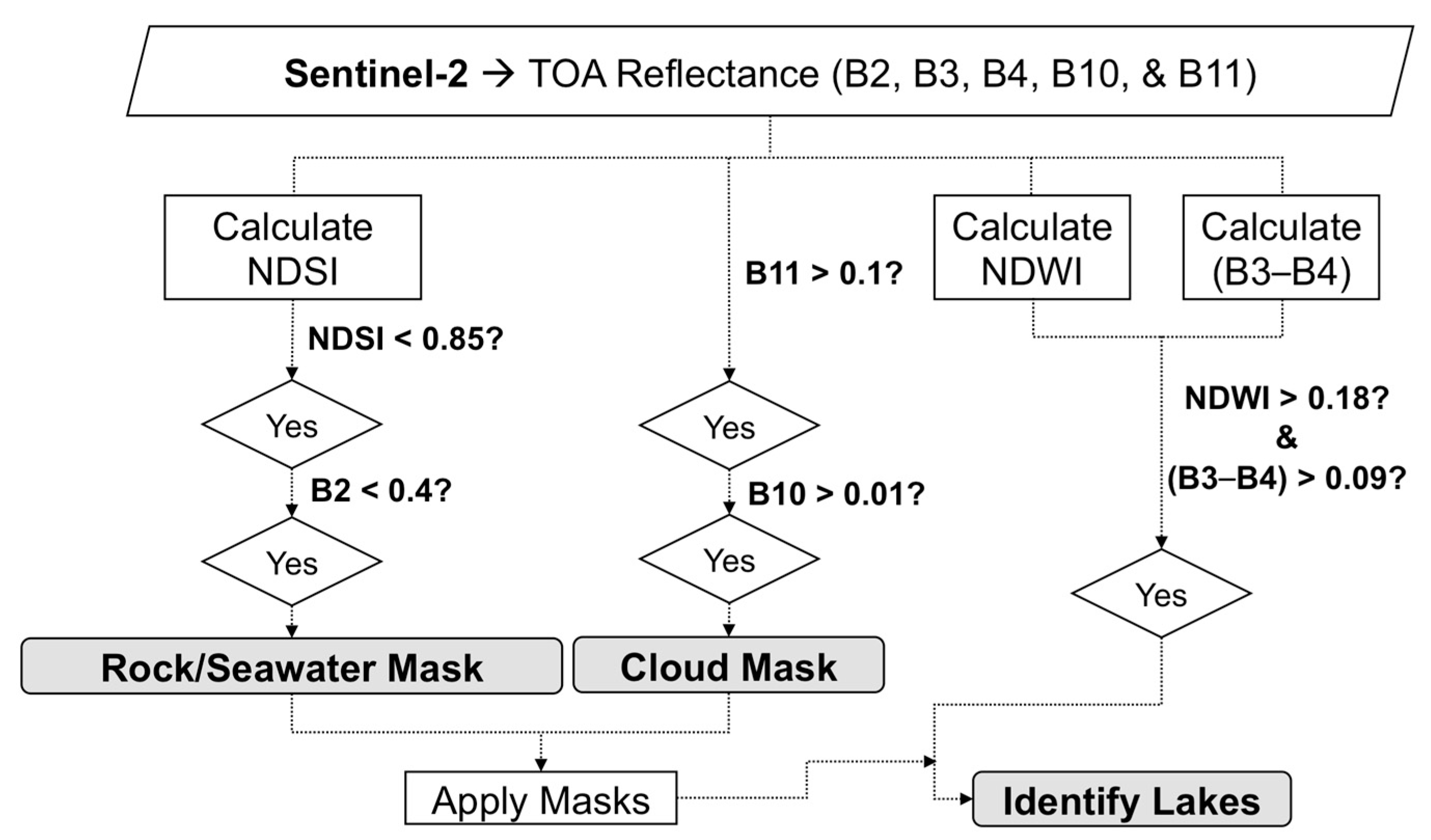
2.3.1. Threshold-Based Classification of Lakes, Rocks, and Clouds
Landsat 8
Sentinel-2
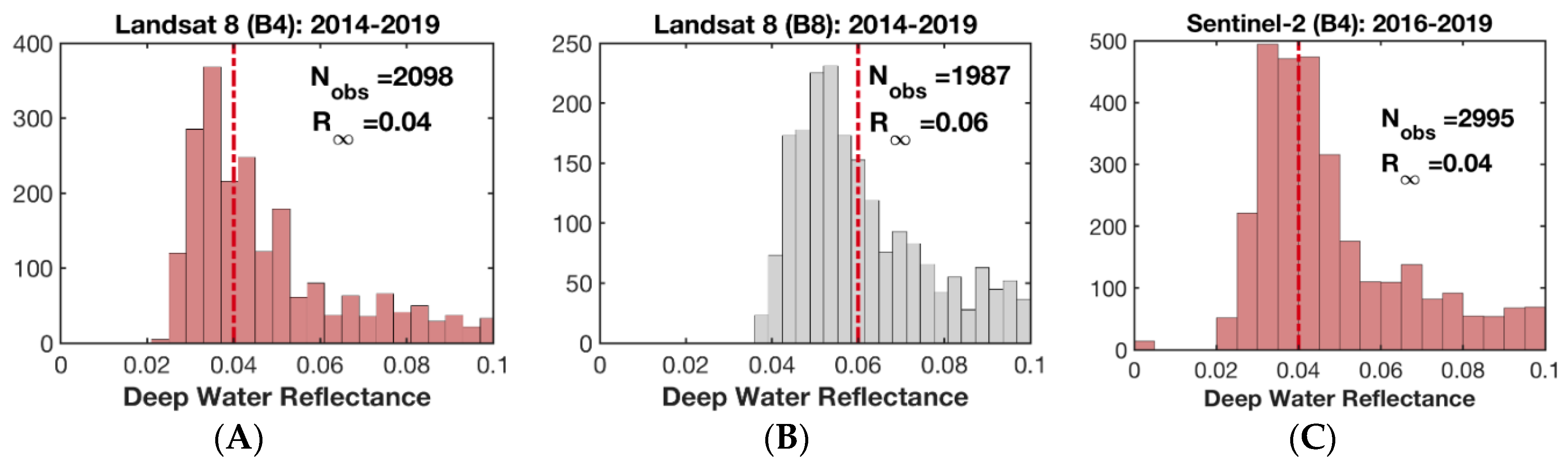
2.4. Lake Depth Retrieval and Volume Estimation
2.4.1. Landsat 8
2.4.2. Sentinel-2
3. Results
3.1. Assessment of Lake Extents
3.1.1. Visual Inspection of Results across 1000 Images and Four Ice Shelves
3.1.2. Comparison with Manually-Digitized Lake Polygons
3.1.3. Comparisons with Other Methods
3.1.4. Cross-Validation of Landsat 8 and Sentinel-2 Derived Lake Areas and Depths
4. Discussion
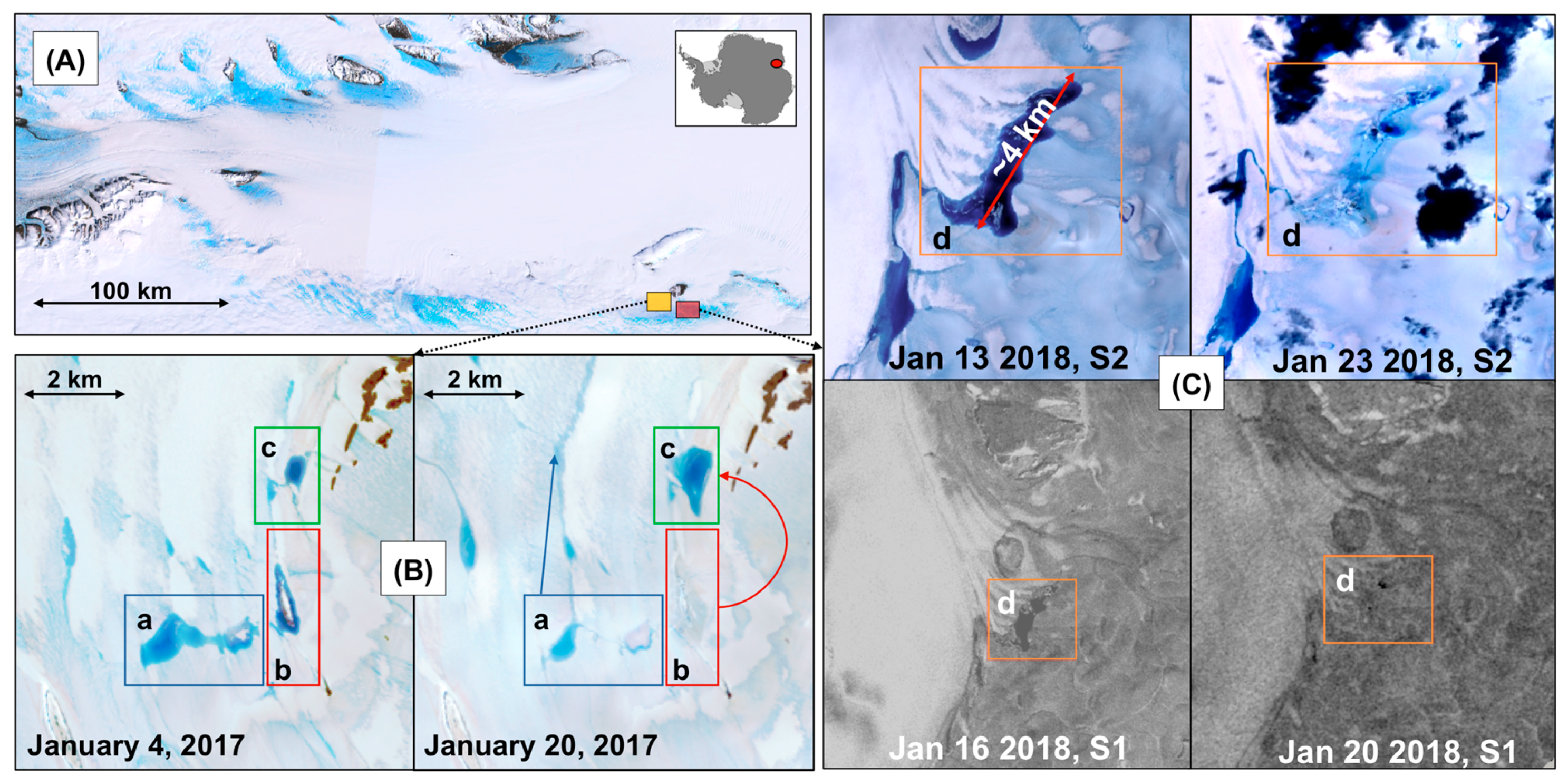
4.1. Lake Drainage Events on the Amery Ice Shelf
4.2. Lake Evolution
5. Conclusions
Author Contributions
Funding
Conflicts of Interest
References
- Sundal, A.V.; Shepherd, A.; Nienow, P.; Hanna, E.; Palmer, S.; Huybrechts, P. Evolution of supra-glacial lakes across the Greenland Ice Sheet. Remote Sens. Environ. 2009, 113, 2164–2171. [Google Scholar] [CrossRef]
- Selmes, N.; Murray, T.; James, T.D. Fast draining lakes on the Greenland Ice Sheet. Geophys. Res. Lett. 2011, 38. [Google Scholar] [CrossRef]
- Liang, Y.-L.; Colgan, W.; Lv, Q.; Steffen, K.; Abdalati, W.; Stroeve, J.; Gallaher, D.; Bayou, N. A decadal investigation of supraglacial lakes in West Greenland using a fully automatic detection and tracking algorithm. Remote Sens. Environ. 2012, 123, 127–138. [Google Scholar] [CrossRef]
- Morriss, B.F.; Hawley, R.L.; Chipman, J.W.; Andrews, L.C.; Catania, G.A.; Hoffman, M.J.; Lüthi, M.P.; Neumann, T.A. A ten-year record of supraglacial lake evolution and rapid drainage in West Greenland using an automated processing algorithm for multispectral imagery. Cryosphere 2013, 7, 1869–1877. [Google Scholar] [CrossRef]
- Pope, A.; Scambos, T.A.; Moussavi, M.; Tedesco, M.; Willis, M.; Shean, D.; Grigsby, S. Estimating supraglacial lake depth in West Greenland using Landsat 8 and comparison with other multispectral methods. Cryosphere 2016, 10, 15–27. [Google Scholar] [CrossRef]
- Moussavi, M.S.; Abdalati, W.; Pope, A.; Scambos, T.; Tedesco, M.; MacFerrin, M.; Grigsby, S. Derivation and validation of supraglacial lake volumes on the Greenland Ice Sheet from high-resolution satellite imagery. Remote Sens. Environ. 2016, 183, 294–303. [Google Scholar] [CrossRef]
- Banwell, A.F.; Caballero, M.; Arnold, N.S.; Glasser, N.F.; Cathles, L.M.; MacAyeal, D.R. Supraglacial lakes on the Larsen B ice shelf, Antarctica, and at Paakitsoq, West Greenland: A comparative study. Ann. Glaciol. 2014, 55, 1–8. [Google Scholar] [CrossRef]
- Zwally, H.J.; Abdalati, W.; Herring, T.; Larson, K.; Saba, J.; Steffen, K. Surface Melt-Induced Acceleration of Greenland Ice-Sheet Flow. Science 2002, 297, 218–222. [Google Scholar] [CrossRef]
- Bartholomew, I.D.; Nienow, P.; Sole, A.; Mair, D.; Cowton, T.; King, M.A.; Palmer, S. Seasonal variations in Greenland Ice Sheet motion: Inland extent and behaviour at higher elevations. Earth Planet. Sci. Lett. 2011, 307, 271–278. [Google Scholar] [CrossRef]
- Bartholomew, I.; Nienow, P.; Sole, A.; Mair, D.; Cowton, T.; King, M.A. Short-term variability in Greenland Ice Sheet motion forced by time-varying meltwater drainage: Implications for the relationship between subglacial drainage system behavior and ice velocity. J. Geophys. Res. 2012, 117. [Google Scholar] [CrossRef]
- Hoffman, M.J.; Catania, G.A.; Neumann, T.A.; Andrews, L.C.; Rumrill, J.A. Links between acceleration, melting, and supraglacial lake drainage of the western Greenland Ice Sheet. J. Geophys. Res. 2011, 116. [Google Scholar] [CrossRef]
- Smith, L.C.; Chu, V.W.; Yang, K.; Gleason, C.J.; Pitcher, L.H.; Rennermalm, A.K.; Legleiter, C.J.; Behar, A.E.; Overstreet, B.T.; Moustafa, S.E.; et al. Efficient meltwater drainage through supraglacial streams and rivers on the southwest Greenland ice sheet. Proc. Natl. Acad. Sci. USA 2015, 112, 1001–1006. [Google Scholar] [CrossRef] [PubMed]
- Yang, K.; Smith, L.C. Supraglacial Streams on the Greenland Ice Sheet Delineated from Combined Spectral–Shape Information in High-Resolution Satellite Imagery. IEEE Geosci. Remote Sens. Lett. 2013, 10, 801–805. [Google Scholar] [CrossRef]
- Legleiter, C.J.; Tedesco, M.; Smith, L.C.; Behar, A.E.; Overstreet, B.T. Mapping the bathymetry of supraglacial lakes and streams on the Greenland ice sheet using field measurements and high-resolution satellite images. Cryosphere 2014, 8, 215–228. [Google Scholar] [CrossRef]
- Fetterer, F.; Untersteiner, N. Observations of melt ponds on Arctic sea ice. J. Geophys. Res. 1998, 103, 24821–24835. [Google Scholar] [CrossRef]
- Scambos, T.A.; Bohlander, J.A.; Shuman, C.A.; Skvarca, P. Glacier acceleration and thinning after ice shelf collapse in the Larsen B embayment, Antarctica. Geophys. Res. Lett. 2004, 31. [Google Scholar] [CrossRef]
- Scambos, T.; Fricker, H.A.; Liu, C.-C.; Bohlander, J.; Fastook, J.; Sargent, A.; Massom, R.; Wu, A.-M. Ice shelf disintegration by plate bending and hydro-fracture: Satellite observations and model results of the 2008 Wilkins ice shelf break-ups. Earth Planet. Sci. Lett. 2009, 280, 51–60. [Google Scholar] [CrossRef]
- Shuman, C.A.; Berthier, E.; Scambos, T.A. 2001–2009 elevation and mass losses in the Larsen A and B embayments, Antarctic Peninsula. J. Glaciol. 2011, 57, 737–754. [Google Scholar] [CrossRef][Green Version]
- Glasser, N.F.; Scambos, T.A. A structural glaciological analysis of the 2002 Larsen B ice-shelf collapse. J. Glaciol. 2008, 54, 3–16. [Google Scholar] [CrossRef]
- Banwell, A.F.; Macayeal, D.R. Ice-shelf fracture due to viscoelastic flexure stress induced by fill/drain cycles of supraglacial lakes. Antarct. Sci. 2015, 27, 587–597. [Google Scholar] [CrossRef]
- Kingslake, J.; Ely, J.C.; Das, I.; Bell, R.E. Widespread movement of meltwater onto and across Antarctic ice shelves. Nature 2017, 544, 349–352. [Google Scholar] [CrossRef] [PubMed]
- Stokes, C.R.; Sanderson, J.E.; Miles, B.W.J.; Jamieson, S.S.R.; Leeson, A.A. Widespread distribution of supraglacial lakes around the margin of the East Antarctic Ice Sheet. Sci. Rep. 2019, 9, 1–14. [Google Scholar] [CrossRef] [PubMed]
- Williamson, A.G.; Willis, I.C.; Arnold, N.S.; Banwell, A.F. Controls on rapid supraglacial lake drainage in West Greenland: An Exploratory Data Analysis approach. J. Glaciol. 2018, 64, 208–226. [Google Scholar] [CrossRef]
- Tedesco, M.; Steiner, N. In-situ multispectral and bathymetric measurements over a supraglacial lake in western Greenland using a remotely controlled watercraft. Cryosphere 2011, 5, 445–452. [Google Scholar] [CrossRef]
- Box, J.E.; Ski, K. Remote sounding of Greenland supraglacial melt lakes: Implications for subglacial hydraulics. J. Glaciol. 2007, 53, 257–265. [Google Scholar] [CrossRef]
- Sneed, W.A.; Hamilton, G.S. Evolution of melt pond volume on the surface of the Greenland Ice Sheet. Geophys. Res. Lett. 2007, 34. [Google Scholar] [CrossRef]
- Burton-Johnson, A.; Black, M.; Fretwell, P.T.; Kaluza-Gilbert, J. An automated methodology for differentiating rock from snow, clouds and sea in Antarctica from Landsat 8 imagery: A new rock outcrop map and area estimation for the entire Antarctic continent. Cryosphere 2016, 10, 1665–1677. [Google Scholar] [CrossRef]
- Mellor, M. Antarctic Ice Terminology: Ice Dolines1. Polar Rec. 1960, 10, 92. [Google Scholar] [CrossRef]
- Charles, S. Satellite Image Atlas of Glaciers of of the World—Antarctica; Williams, R.S., Ferrigno, J.G., Eds.; Unites States Government Printing Office: Washington, DC, USA, 1988; Volume 1386B.
- Trusel, L.D.; Frey, K.E.; Das, S.B.; Munneke, P.K.; Broeke, M.R. van den Satellite-based estimates of Antarctic surface meltwater fluxes. Geophys. Res. Lett. 2013, 40, 6148–6153. [Google Scholar] [CrossRef]
- Kingslake, J.; Ng, F.; Sole, A. Modelling channelized surface drainage of supraglacial lakes. J. Glaciol. 2015, 61, 185–199. [Google Scholar] [CrossRef]
- Langley, E.S.; Leeson, A.A.; Stokes, C.R.; Jamieson, S.S.R. Seasonal evolution of supraglacial lakes on an East Antarctic outlet glacier. Geophys. Res. Lett. 2016, 43, 8563–8571. [Google Scholar] [CrossRef]
- Lenaerts, J.T.M.; Lhermitte, S.; Drews, R.; Ligtenberg, S.R.M.; Berger, S.; Helm, V.; Smeets, C.J.P.P.; Van den Broeke, M.R.; Van De Berg, W.J.; Van Meijgaard, E.; et al. Meltwater produced by wind–albedo interaction stored in an East Antarctic ice shelf. Nat. Clim. Chang. 2017, 7, 58–62. [Google Scholar] [CrossRef]
- Fricker, H.A.; Hyland, G.; Coleman, R.; Young, N.W. Digital elevation models for the Lambert Glacier–Amery Ice Shelf system, East Antarctica, from ERS-1 satellite radar altimetry. J. Glaciol. 2000, 46, 553–560. [Google Scholar] [CrossRef]
- Bindschadler, R.; Vornberger, P.; Fleming, A.; Fox, A.; Mullins, J.; Binnie, D.; Paulsen, S.J.; Granneman, B.J.; Gorodetzky, D. The Landsat Image Mosaic of Antarctica. Remote Sens. Environ. 2008, 112, 13. [Google Scholar] [CrossRef]
- Halberstadt, A.R.; Moussavi, M.S.; Pope, A.; Gleason, C.J.; Trusel, L.D.; DeConto, R.M. Antarctic supraglacial lake identification using supervised image classification. Unpublished work. 2019. [Google Scholar]
- Macdonald, G.J.; Banwell, A.F.; MacAyeal, D.R. Seasonal evolution of supraglacial lakes on a floating ice tongue, Petermann Glacier, Greenland. Ann. Glaciol. 2018, 59, 56–65. [Google Scholar] [CrossRef]
- Miles, K.E.; Willis, I.C.; Benedek, C.L.; Williamson, A.G.; Tedesco, M. Toward Monitoring Surface and Subsurface Lakes on the Greenland Ice Sheet Using Sentinel-1 SAR and Landsat-8 OLI Imagery. Front. Earth Sci. 2017, 5, 58. [Google Scholar] [CrossRef]
- Hall, D.K.; Riggs, G.A.; Salomonson, V.V. Development of methods for mapping global snow cover using moderate resolution imaging spectroradiometer data. Remote Sens. Environ. 1995, 54, 127–140. [Google Scholar] [CrossRef]
- Dozier, J. Spectral signature of alpine snow cover from the landsat thematic mapper. Remote Sens. Environ. 1989, 28, 9–22. [Google Scholar] [CrossRef]
- Williamson, A.G.; Banwell, A.F.; Willis, I.C.; Arnold, N.S. Dual-satellite (Sentinel-2 and Landsat 8) remote sensing of supraglacial lakes in Greenland. Cryosphere 2018, 12, 3045–3065. [Google Scholar] [CrossRef]
- Philpot, W.D. Bathymetric mapping with passive multispectral imagery. Appl. Opt. 1989, 28, 1569. [Google Scholar] [CrossRef]
- Broeke, M. van den Strong surface melting preceded collapse of Antarctic Peninsula ice shelf. Geophys. Res. Lett. 2005, 32. [Google Scholar] [CrossRef]
- Banwell, A.F.; MacAyeal, D.R.; Sergienko, O.V. Breakup of the Larsen B Ice Shelf triggered by chain reaction drainage of supraglacial lakes. Geophys. Res. Lett. 2013, 40, 5872–5876. [Google Scholar] [CrossRef]
- MacAyeal, D.R.; Sergienko, O.V. The flexural dynamics of melting ice shelves. Ann. Glaciol. 2013, 54, 1–10. [Google Scholar] [CrossRef]
- Bell, R.E.; Banwell, A.F.; Trusel, L.D.; Kingslake, J. Antarctic surface hydrology and impacts on ice-sheet mass balance. Nat. Clim Chang. 2018, 8, 1044–1052. [Google Scholar] [CrossRef]
- Tuckett, P.A.; Ely, J.C.; Sole, A.J.; Livingstone, S.J.; Davison, B.J.; van Wessem, J.M.; Howard, J. Rapid accelerations of Antarctic Peninsula outlet glaciers driven by surface melt. Nat. Commun. 2019, 10, 1–8. [Google Scholar] [CrossRef] [PubMed]
- Beltaos, S. Collapse of floating ice covers under vertical loads: Test data vs. theory. Cold Reg. Sci. Technol. 2002, 34, 191–207. [Google Scholar] [CrossRef]
- Banwell, A.F.; Willis, I.C.; Macdonald, G.J.; Goodsell, B.; MacAyeal, D.R. Direct measurements of ice-shelf flexure caused by surface meltwater ponding and drainage. Nat. Commun. 2019, 10, 730. [Google Scholar] [CrossRef]


| Validation Site | Landsat 8/Sentinel-2 Scene | Accuracy |
|---|---|---|
| Roi Baudouin Ice Shelf | LC08_L1GT_154109_20140116 | 99.6% |
| LC08_L1GT_154109_20170225 | 99.0% | |
| LC08_L1GT_154109_20180111 | 95.5% | |
| Amery Ice Shelf | LC08_L1GT_127111_20140204 | 97.9% |
| LC08_L1GT_127111_20161226 | 98.0% | |
| LC08_L1GT_127111_20140204 | 94.7% | |
| S2B_MSIL1C_20190102T041719_N0207_R061_T41CPV | 97.8% | |
| S2B_MSIL1C_20190102T041719_N0207_R061_T41DPA | 96.5% | |
| S2B_MSIL1C_20190113T034629_N0207_R075_T42DWF | 98.4% | |
| Total traced lake area (Landsat 8) | ~340 km2 | |
| Total traced lake area (Sentinel-2) | ~190 km2 | |
| Average Accuracy (Landsat 8) | ~94.5% | |
| Average Accuracy (Sentinel-2) | ~97.5% |
| Site | Landsat 8 | Sentinel-2 | Volumetric Difference (%) | Dice Similarity Coefficient | ||||
|---|---|---|---|---|---|---|---|---|
| Date | Mean Depth (m) | Total Volume (× 106 m3) | Date | Mean Depth (m) | Total Volume (× 106 m3) | |||
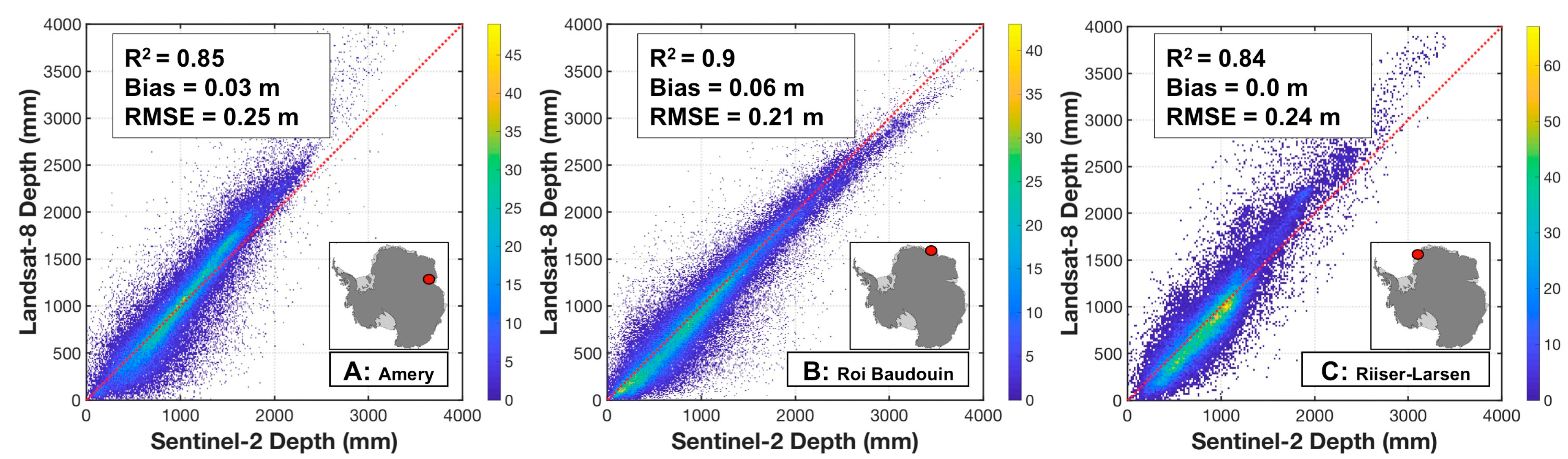
| Amery (1) | 23 January 2018 | 0.96 | 99 | 23 January 2018 | 0.95 | 97 | 2 | 0.82 |
| Roi Baudouin | 14 January 2019 | 0.89 | 0.36 | 14 January 2019 | 0.98 | 0.38 | 0 | 0.80 |
| Amery (2) | 3 January 2019 | 0.87 | 116 | 3 January 2019 | 0.94 | 123 | −5 | 0.82 |
| Riiser-Larsen | 1 February 2017 | 0.85 | 43 | 2 February 2017 | 0.87 | 43 | 0 | 0.88 |
| Lake | Mean Depth (m) | Area (km2) | Volume (× 106 m) | |||
|---|---|---|---|---|---|---|
| 4 January 2017 | 20 January 2017 | 4 January 2017 | 20 January 2017 | 4 January 2017 | 20 January 2017 | |
| a | 1 | 0.7 | 1.1 | 0.3 | 1.1 | 0.25 |
| b | 1.3 | ~0 | 0.4 | ~0 | 0.5 | ~0 |
| c | 1.5 | 1.4 | 0.2 | 0.8 | 0.3 | 1.13 |
| d | 2 | ~0 | 4.3 | ~0 | 8.6 | ~0 |
© 2020 by the authors. Licensee MDPI, Basel, Switzerland. This article is an open access article distributed under the terms and conditions of the Creative Commons Attribution (CC BY) license (http://creativecommons.org/licenses/by/4.0/).
Share and Cite
Moussavi, M.; Pope, A.; Halberstadt, A.R.W.; Trusel, L.D.; Cioffi, L.; Abdalati, W. Antarctic Supraglacial Lake Detection Using Landsat 8 and Sentinel-2 Imagery: Towards Continental Generation of Lake Volumes. Remote Sens. 2020, 12, 134. https://doi.org/10.3390/rs12010134
Moussavi M, Pope A, Halberstadt ARW, Trusel LD, Cioffi L, Abdalati W. Antarctic Supraglacial Lake Detection Using Landsat 8 and Sentinel-2 Imagery: Towards Continental Generation of Lake Volumes. Remote Sensing. 2020; 12(1):134. https://doi.org/10.3390/rs12010134
Chicago/Turabian StyleMoussavi, Mahsa, Allen Pope, Anna Ruth W. Halberstadt, Luke D. Trusel, Leanne Cioffi, and Waleed Abdalati. 2020. "Antarctic Supraglacial Lake Detection Using Landsat 8 and Sentinel-2 Imagery: Towards Continental Generation of Lake Volumes" Remote Sensing 12, no. 1: 134. https://doi.org/10.3390/rs12010134
APA StyleMoussavi, M., Pope, A., Halberstadt, A. R. W., Trusel, L. D., Cioffi, L., & Abdalati, W. (2020). Antarctic Supraglacial Lake Detection Using Landsat 8 and Sentinel-2 Imagery: Towards Continental Generation of Lake Volumes. Remote Sensing, 12(1), 134. https://doi.org/10.3390/rs12010134