Multi-View Features Joint Learning with Label and Local Distribution Consistency for Point Cloud Classification

Abstract

In outdoor Light Detection and Ranging (lidar)point cloud classification, finding the discriminative features for point cloud perception and scene understanding represents one of the great challenges. The features derived from defect-laden (i.e., noise, outliers, occlusions and irregularities) and raw outdoor LiDAR scans usually contain redundant and irrelevant information which adversely affects the accuracy of point semantic labeling. Moreover, point cloud features of different views have a capability to express different attributes of the same point. The simplest way of concatenating these features of different views cannot guarantee the applicability and effectiveness of the fused features. To solve these problems and achieve outdoor point cloud classification with fewer training samples, we propose a novel multi-view features and classifiers’ joint learning framework. The proposed framework uses label consistency and local distribution consistency of multi-space constraints for multi-view point cloud features extraction and classification. In the framework, the manifold learning is used to carry out subspace joint learning of multi-view features by introducing three kinds of constraints, i.e., local distribution consistency of feature space and position space, label consistency among multi-view predicted labels and ground truth, and label consistency among multi-view predicted labels. The proposed model can be well trained by fewer training points, and an iterative algorithm is used to solve the joint optimization of multi-view feature projection matrices and linear classifiers. Subsequently, the multi-view features are fused and used for point cloud classification effectively. We evaluate the proposed method on five different point cloud scenes and experimental results demonstrate that the classification performance of the proposed method is at par or outperforms the compared algorithms.

1. Introduction

In recent years, with the rapid advancement of computer vision and Light Detection and Ranging (lidar) technology, an increasing number of point clouds are acquired and widely used in various remote-sensing applications. In applications such as autonomous driving, understanding the outdoor scenes by semantic labeling of point clouds has become a hot topic [1,2,3,4]. Point cloud classification is to mark a specific semantic attribute label for each point in the point cloud [2], which is a key step in environmental perception and scene understanding. Due to disorder, sparsity and irregularity of point clouds as well as the possible presence of uncertainty in point clouds (noise, outliers and missing data), the intra-class points in the same scene are quite different and the difference of inter-class points is not obvious [3]. Therefore, effective classification of point clouds is a challenging problem.

For the past few years, the classification algorithms proposed in [3,4,5,6,7,8,9] have achieved good performances for classifying images and point clouds. For example, Zhang et al. [10] proposed DKSVD (discriminative K-SVD [11]) algorithm, which introduces classification error to optimize feature extraction and classifier, simultaneously. To explore prior knowledge of label information, Jiang et al. [12] introduced label consistency constraints into the objective functions of LCKSVD1 (Label Consistent K-SVD) and LCKSVD2 algorithms, and showed better classification results. Zhang et al. [1] used discriminant dictionary learning to construct multi-level point set features for point cloud classification. Li et al. [4] proposed a deep-learning network based on multi-level voxel features fusion for point cloud classification. The feature dimensions used by the above methods are relatively high, and are found to be carrying noise and redundant information [13]. To overcome this drawback, dimensionality reduction and sparse representation are widely used. Dimensionality reduction can be seen as a special case of subspace learning, which projects high-dimensional data to low-dimensional subspace through algorithms, such as ICA (independent component analysis) [14], PCA (principal component analysis) [15], optimal mean robust PCA [16] and other variants.

In addition, most supervised classification methods usually require a huge amount of training samples to learn features and classifiers to achieve very high classification accuracy. As the training set generation through point cloud labeling is time-consuming, it significantly lowers the algorithmic efficiency [17]. Therefore, if we can successfully classify a large volumes of point clouds using only a small percentage of training samples, it should have a great practical applicability because the time and labor cost will be significantly reduced [5]. To solve this problem, [13,17,18,19] proposed semi-supervised or supervised classification methods for feature transformation matrix and classifier joint learning. For example, Mei et al. [17] concatenated multiple single point features to form high-dimensional features for each point, and then used the joint constraints of margin, graph of adjacency and labels to train the model with a small portion of samples based on a semi-supervised framework. Zhu et al. [18] used the feature vector composed of multi-scale features in a series of images to express each image, and then the constraints of local connection relations of labels and samples were introduced to jointly learn the features projection matrix and classifier with local and global consistency. These methods directly fuse different types of sample features or the same features defined at multiple scales for classification. However, this kind of feature fusion and its variants have relatively limited expression ability of sample attributes and classification performances. In this case, the effectiveness of feature fusion cannot be guaranteed.

To express and classify multimedia data effectively, researchers have proposed a variety of multi-view learning algorithms. Each point can be described by high-dimensional features from multiple views, e.g., eigenvalue features of covariance matrix [1], spin image features [20], normal vector, FPFH (fast-point feature histogram) [21] and VFH (viewpoint feature histogram) [22]. The created features in each view contain unique information that is different from the features derived from other views. Meanwhile, it should be noted that multi-view features also include some overlapping information to a certain extent, although they are generalized from different views. Different view features describe properties of different aspects of a point, but they commonly represent the same point. Typically, the multi-view learning methods [23,24,25,26,27,28,29,30,31] can effectively fuse features from different views. The authors leverage this diversity and consistency of different view features to obtain more discriminative feature representation. More specifically, Nie et al. [25] proposed an adaptive weighted multi-view learning algorithm (MLAN) for image clustering and semi-supervised classification. This algorithm introduces different view weights and learns the local structure from different view data based on a manifold learning method. In [28], the features’ low-rank representations of each view are jointly optimized by introducing the exclusivity and category consistency constraints. In contrast to [28], the method in [31] jointly learned the low-rank representations of multi-view by introducing the error term with adaptive weight of each view and the diversity regular term for reducing redundant information between different views. Then, the joint projection graph of the multi-view was constructed by the low-rank representations for clustering/classification. All these methods outperform the single-view feature-learning methods, however, they are not applicable for classifying outdoor point clouds. By contrast with the above multi-view learning methods, some multi-view Convolutional Neural Networks (CNNs) based methods (deep learning mechanism) for point cloud processing are proposed in recent years [32]. Generally, this kind of method relies on 2D rendered views instead of on the 3D data. For example, Su et al. [33] use multi-view CNNs to extract the features of 2D renderings from a 3D object, which shows good performance for 3D object model classification. For point cloud semantic segmentation of outdoor scenes, multi-view CNN-based methods, e.g., [34,35,36], need to render point cloud to generate multi-view images with multi-modal representation, which can include the information of depth, color, normal and other features. Then the generated multiple images are semantically segmented by the networks, e.g., U-Net [37], SegNet [38] and Fully Convolutional Network (FCN) [39]. After that, the semantic segmentation results of multiple images are projected to meshes to jointly determine the label of each mesh vertex. Finally, the labeled vertices are projected to the original point cloud. Although these deep learning-based methods have been obtaining good results, they rely on full 3D meshes to generate multi-view rendering, which is difficult to enable the reliable 3D meshes for outdoor point clouds. These multi-view methods are processed based on images, not 3D point clouds. In addition, to the best of our knowledge, there does not exist any multi-view learning method that is directly applied to point cloud classification.

To fill this gap, we propose a features extraction and point clouds classification model based on multiple views and space representation consistency under constraints of label consistency (MvsRCLC). The overall flowchart of the proposed algorithm is shown in Figure 1. Firstly, the multi-view features of each point are extracted. Then, the features of each view are joined to learn the subspace of each view to remove redundant information, making the features representation more suitable for classification tasks. Secondly, the local distribution consistency constraint of feature space and position space is used to express the adjacency graph of each point in the local neighborhood. After that, the label consistency constraint is used to ensure the consistency between the predicted labels of all views and the ground truth label, as well as the consistency between the predicted labels within multiple views. Label consistency includes label consistency of grouped points (LCG) and label consistency of single point (LCS). Finally, an iterative optimization algorithm of objective function is proposed to progressively learn a subspace projection matrix and optimal linear classifier via solving a minimization problem. In the experimental section, two airborne laser-scanning (ALS) data scenes, two mobile laser-scanning (MLS) scenes and a terrestrial laser-scanning (TLS) scene with different complexities are used to evaluate the proposed algorithm.

We state the original contributions explicitly as below:

(1) A multi-view features and classifiers fusion framework for point cloud classification is proposed. By introducing the multiple constraints among different views and combining the classification error terms, the feature subspaces of multi-view can be jointly learned. This subspace learning method can be used to remove redundant information or noise effectively. Moreover, by simultaneously optimizing the feature projection matrices and linear classifiers of all views on the unified objective function, different view features can be fully explored, and more discriminant feature subspaces and optimal linear classifiers can be obtained.

(2) Unlike previous methods that simply concatenate multi-view features for classification, we propose a multi-view subspace learning method using diversity and consistency constraints between multi-view features, and then multi-view features and the classifier are coupled to classify point clouds, thereby improving labeling accuracy.

(3) Our algorithm takes multiple constraints including, local distribution consistency in feature space and position space, LCG constraints and predicted labels consistency constraints of multi-view features into account. It enhances subspace representations of point clouds and improves classification accuracy of point clouds. The proposed method has better classification performances particularly for using a small portion of training samples.

(4) The joint optimization method of multi-view objective function based on an iterative algorithm proposed in this paper can rapidly converge on the point cloud scenes used in this paper. The proposed algorithm is superior to other state-of-the-art methods by labeling ubiquitous points, ALS, MLS and TLS point clouds.

2. Materials and Methods

In this section, the multi-view point features, i.e., normal vector, covariance eigenvalue features and spin image features, used in our method are firstly presented. Then, the joint learning of the multi-view point feature extraction and classification model is constructed, which mainly includes: subspace learning, local distribution consistency constraint of multi-view feature and position spaces, and multi-view label constraints. Next, the proposed model is optimized before it is used to classify point clouds.

2.1. Multi-View Point Cloud Feature Extraction

The different types of features represent different attributes of point clouds. Thus, we extract different types of point cloud features to fully express point cloud attributes. In this paper, point cloud features of different views are constructed by using normal vector ${\mathbf{F}}^{nor}$, covariance eigenvalue features ${\mathbf{F}}^{cov}$ [1] and spin image features ${\mathbf{F}}^{spin}$ [20]. Here, we also generate a series of single point features extracted at multi-scale regions to enhance object recognition abilities. The features extraction processes are described as follows:

The neighborhood points of point p in radius r is regarded as the support region of point p. We construct the features defined at different scales by progressively changing radius r. Different radii r are selected to construct features of different scales for each view. The normal vector and covariance eigenvalue are calculated according to the methods in [3]. Since the normal vector and covariance eigenvalue features mainly represent the geometric features of point cloud, we take them as the same view features. Therefore, the multi-scale features of point clouds belonging to different views constructed by our method is $X={\left[X_1,X_2\right]}^T$, where, $X_1=[{\mathbf{F}}^{cov},{\mathbf{F}}^{nor}] \mathrm{and} X_2={\mathbf{F}}^{spin}$. $X_1$ and $X_2$ represent the features of view 1 and the view 2, respectively. It is to be noted that normal vector, covariance eigenvalue features and spin image features are taken as an example for the proposed method. This means other kinds of features can be used to construct the multi-view features, i.e., the multi-view features $X$ = ${\left[X_1,\dots ,X_m\right]}^T$ (m is the number of views, m > 2) include m kind of features. $X_v$(v $\in \left[1,m\right]$) is the vth view feature.

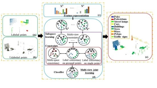
2.2. Multiple Views and Space Representation Consistency under Constraints of Label Consistency (MvsRCLC)

In this section, we discuss multiple views and spaces representations consistency with label consistency constraints for features extraction and point clouds classification (MvsRCLC).

2.2.1. Reconstruction Independent Component Analysis (RICA) Subspace Learning

In the multi-scale point cloud features representation, redundant and/or noisy information is usually present. To solve this problem, the feature projection technique is usually employed. It transforms the data in the high-dimensional space into a lower-dimensional space to achieve dimensionality reduction and subspace learning. To project the high-dimensional features into subspace by the feature transformation matrix with less reconstruction error, MvsRCLC minimizes the following objective function using RICA (reconstruction independent component analysis) algorithm [14] to extract the optimal feature transformation matrix.

$${\Theta }_1(W)=\parallel W^{T}WX-X{\parallel }_F^2+\alpha .g(WX)$$

(1)

where $W\in {ℛ}^{d^{\prime }\times d}$ is the feature transformation matrix that projects $X\in {ℛ}^{d\times n}$ onto a $d^{\prime }$-dimensional feature space ($d^{\prime }<d$). In Equation (1), $g(·)=\log (\cosh (·))\left[13\right],\mathrm{where}\cos \mathrm{h}(WX)=(\exp (WX)+\exp (-WX))/2$, and $\alpha$ is a trade-off factor that is used to balance the reconstruction error term and sparse representation term.

For multi-view features, different views can be projected to the same subspace through different feature transformation matrices. Therefore, the subspace learning objective function of the multi-view features can be defined as:

$${\Theta }_1^v(W_v)={\displaystyle \sum }_{v=1}^m\parallel W_v{}^T{W}_v{X}_v-X_v{\parallel }_F^2+\alpha .g(W_v{X}_v)$$

(2)

where, $W_v$ is the vth view feature transformation matrix, and $X_v$ is the vth feature. m is the number of views.

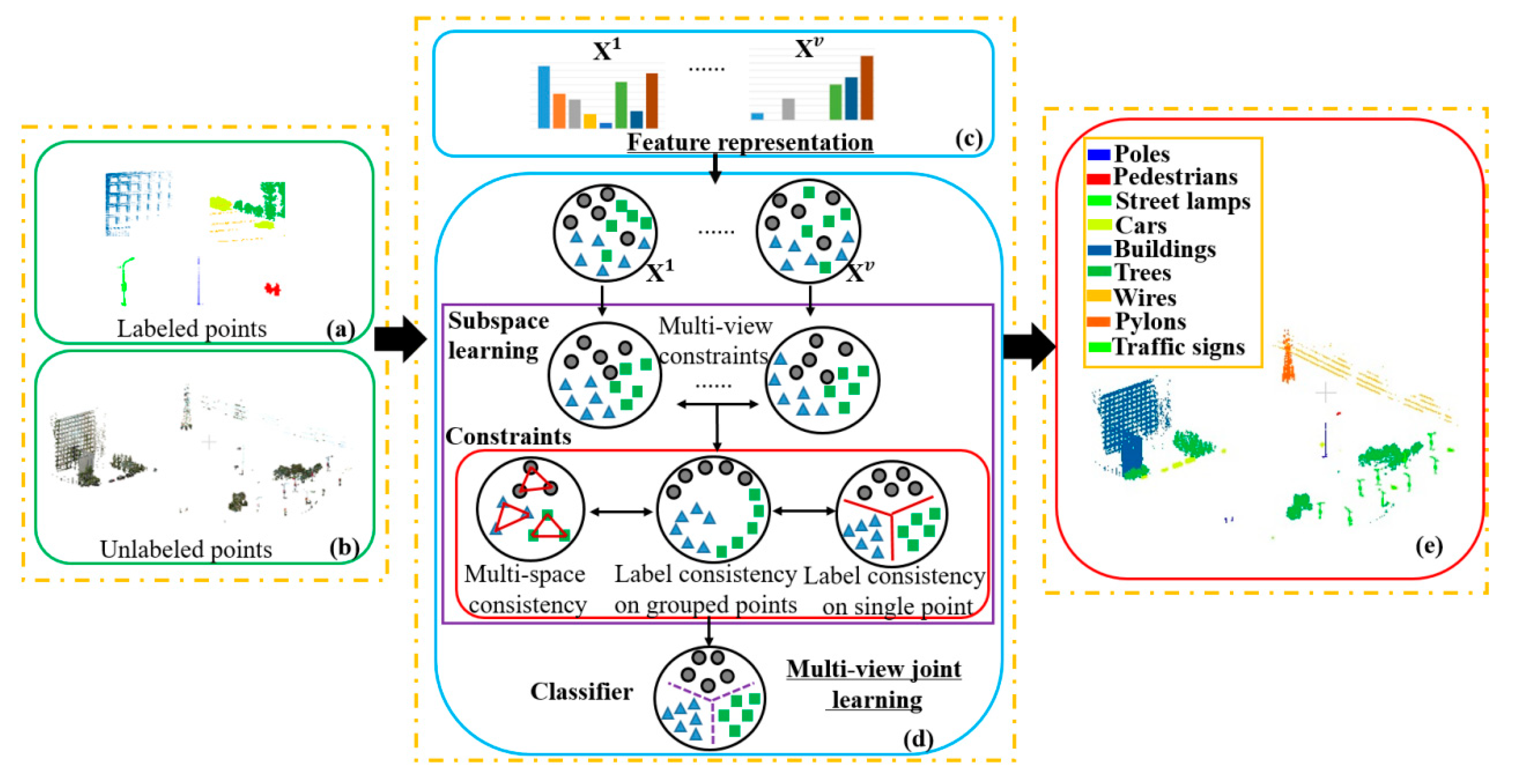
2.2.2. Multi-View Local Distribution Consistency Constraints

(1) Point Cloud Spatial Position Constraint Term

Although each point has different view features, the intrinsic spatial relationships are explicitly embedded in the point clouds. Therefore, the constructed spatial position constraint is applicable to subspace learning of all the views. Intuitively, for point cloud data, K neighbor points in the spatial position space tend to belong to the same category, and points of the same category also have similar data distribution in the feature space. Based on this observation, a coordinate distance constraint from each point to its K neighbor points is imposed, which is expressed by a spatial position weight matrix. Thus, the spatial position weight matrix of the point cloud is expressed as follows:

$$V_{ij}=\{\begin{array}{c}\exp (-\frac{\parallel P_i-P_j{\parallel }_2^2}{\sigma }),\hspace{1em}\mathrm{if}\hspace{1em}{p}_i \in {\varkappa }_K^{\mathrm{v}}( p_j ) \mathrm{or} p_j \in {\varkappa }_K^{\mathrm{v}}( p_i )\\ 0\hspace{1em}\hspace{1em}\hspace{1em}\hspace{1em}\hspace{1em}\hspace{1em}\hspace{1em}\hspace{1em}\hspace{1em}\hspace{1em}\hspace{1em}\hspace{1em}\mathrm{otherwise}\end{array}$$

(3)

where, $P_i$ is the coordinate. ${\varkappa }_K^{\mathrm{v}}(·)$ represents the set of the K nearest neighbor points in the spatial position space.

(2) Point Cloud Feature Space Constraint Term

Similarly, in the feature space, K neighbor points tend to express the objects of the same category. Thus, the feature distance constraint from each point to its K neighbor points in feature space can be constructed, which is expressed by a feature space weight matrix. The point cloud feature space weight matrix is constructed below:

$$U_{ij}=\{\begin{array}{c}\exp (-\parallel {(X)}_i-{(X)}_j{\parallel }_2^2), \mathrm{if} p_i \in {\varkappa }_K^{\mathrm{u}}( p_j ) or p_j \in {\varkappa }_K^{\mathrm{u}}( p_i )\\ 0\hspace{1em}\hspace{1em}\hspace{1em}\hspace{1em}\hspace{1em}\hspace{1em}\hspace{1em}\hspace{1em}\hspace{1em}\hspace{1em}\hspace{1em}\hspace{1em}\mathrm{otherwise}\end{array}$$

(4)

where, ${\varkappa }_K^{\mathrm{u}}( p_j )$ represents the nearest K neighbor of point p_j in feature space.

Considering points of the same category also have similar data distribution in the spatial position space and feature space, spatial position space and feature space constraints in the same view can be jointly expressed as Equation (5). More details can be found in [17,18,19].

$${\Theta }_2(W)=\frac{1}{2}{\displaystyle \sum }_{i,j=1}^n(V_{ij}+\beta U_{ij})\parallel {(WX)}_i-{(WX)}_j{\parallel }_2^2=tr((WX)(L_V+\beta L_U){(WX)}^T)$$

(5)

where,$D_U$ and $D_V$ are diagonal matrices, $d_{ii}^{\mathrm{U}}={\displaystyle \sum }_j{U}_{ij}$,$d_{ii}^{\mathrm{V}}={\displaystyle \sum }_j{V}_{ij},L_U=D_U-U_{ij},L_V=D_V-V_{ij}.\mathrm{Operator}$tr(.) is the trace of the matrix. Parameter $\beta$ is the trade-off parameter.

As shown in Figure 2, the same color points belong to the same category in Figure 2a. Figure 2b shows the 5 neighbor points of p₁ (the red point) in spatial position space. Figure 2c shows the different view relationships of the p₁ and its neighbor points in feature space. The weight of each point in the blue circle (Figure 2b) and red circle (Figure 2c) depends on the distance to the p₁. According to Equations (3) and (4), the weight of neighbor points in different spaces can be described by $V_{ij}$ and $U_{ij}$. If the points are not neighbors, the weight values are assigned to 0. Although features of different views have a certain degree of difference, the points from the same category need to have similar adjacent relationships in the feature space of different views. In order to ensure that local points have a similar relationship graph in multi-view features, the relationship graph can be constrained by the features of different views. Figure 2d is the relationship of neighbor points for projection features, which is projected by the constraints of spatial position space and feature space. Generally, the neighbor points in spatial position space and feature space usually belong to the same category, thus, these constraints can guarantee the similarity of projection features for neighbor points. To minimize the feature discrepancy of points in subspace, the joint constraints of spatial position space and feature space are used to construct the multi-view objective function, which is shown as below:

$${\Theta }_2^v(W_v)={\displaystyle \sum }_{v=1}^{m}tr((W_v{X}_v)(L_V +\beta L_{\mathrm{U}}^v){(W_v{X}_v)}^T)$$

(6)

where, $L_{\mathrm{U}}^v$ is the Laplacian matrix of vth in the feature space.

2.2.3. Label Consistency

(1) Label Consistency of Grouped Points (LCG)

It should be remembered that the corresponding labels need to be consistent before and after the feature transformation of the same category points. Based on this constraint, a label matrix Q of grouped points is built. Assuming that, $x_1 \mathrm{and}{x}_2$ belong to the first category, $x_3$ and $x_4$ belong to the second category and $x_5\mathrm{and}{x}_6$ belong to the third category, the matrix Q can be expressed as:

$$\mathbf{Q}=\left[\begin{array}{c}\begin{array}{cc}1& \begin{array}{ccc}1& 0& \begin{array}{ccc}0& 0& 0\end{array}\end{array}\\ 1& \begin{array}{ccc}1& 0& \begin{array}{ccc}0& 0& 0\end{array}\end{array}\end{array}\\ \begin{array}{cc}0& \begin{array}{ccc}0& 1& \begin{array}{ccc}1& 0& 0\end{array}\end{array}\end{array}\\ \begin{array}{cc}0& \begin{array}{ccc}0& 1& \begin{array}{ccc}1& 0& 0\end{array}\end{array}\end{array}\\ \begin{array}{cc}0& \begin{array}{ccc}0& 0& \begin{array}{ccc}0& 1& 1\end{array}\end{array}\end{array}\\ \begin{array}{cc}0& \begin{array}{ccc}0& 0& \begin{array}{ccc}0& 1& 1\end{array}\end{array}\end{array}\end{array}\right]$$

After defining Q, the corresponding objective function of LCG can be expressed as follows:

$${\Theta }_3(G)=\parallel \mathrm{Q}-GWX{\parallel }_F^2+\gamma \parallel G{\parallel }_F^2$$

(7)

where G is the weight matrix, and the term $\gamma \parallel G{\parallel }_F^2$ is the constraint used to prevent overfitting.

In addition, the ground truth labels of grouped points should be consistent with the predicted labels of grouped points at each view, and predicted labels of grouped points between different views are consistent. Therefore, we introduce the difference between the predicted labels of grouped points at different views as a constraint, which can be calculated by $\parallel G_v{W}_v{X}_v-G_w{W}_w{X}_w{\parallel }_F^2$. Then, the corresponding multi-view objective function can be expressed as follows:

$${\Theta }_3^v(G_v)={{\displaystyle \sum }}_{v=1}^m\parallel \mathrm{Q}-G_v{W}_v{X}_v{\parallel }_F^2+\gamma \parallel G_v{\parallel }_F^2 +\delta {{\displaystyle \sum }}_{v\ne w}\parallel G_v{W}_v{X}_v-G_w{W}_w{X}_w{\parallel }_F^2$$

(8)

where, $\gamma \mathrm{and}\delta$ are trade-off parameters.

(2) Label Consistency of Single Point (LCS)

While the classification results between the different views need to be as consistent as possible, each view classification result needs to be close to the ground truth label. After the point cloud feature transformation, the classification results obtained by the linear classifier using the projected features should be consistent with the ground truth. The LCS can be expressed as:

$${\Theta }_4(H)=\parallel \mathbf{F}-HWX{\parallel }_F^2+\gamma \parallel H{\parallel }_F^2$$

(9)

where H is the linear classification matrix, and the term $\gamma \parallel H{\parallel }_F^2$ is the constraint used to prevent overfitting. F is the ground truth label matrix, which is same for all views. To make the predicted labels between the different views consistent, we introduce the discrepancy between the predicted labels of each point at different views as a constraint, which can be calculated by $\parallel H_v{W}_v{X}_v-H_w{W}_w{X}_w{\parallel }_F^2$. Then, the objective function of the multi-view LCS can be expressed as follows:

$${\Theta }_4^v(H_v)={{\displaystyle \sum }}_{v=1}^m\parallel \mathbf{F}-H_v{W}_v{X}_v{\parallel }_F^2+\gamma \parallel H_v{\parallel }_F^2+\delta {{\displaystyle \sum }}_{v\ne w}\parallel H_v{W}_v{X}_v-H_w{W}_w{X}_w{\parallel }_F^2$$

(10)

where, $\gamma \mathrm{and}\delta$ are trade-off parameters.

2.2.4. Objective Function of MvsRCLC

To make the point cloud features with stronger expression ability, MvsRCLC learns the discriminative optimal feature expression through the subspace learning method. To leverage the diversity of subspace feature expressions from different views, joint constraint terms of position space and feature space are introduced. To make sure that the subspace feature expressions of the same category can be consistent in different views, and the subspace feature expression has the best discriminability, MvsRCLC introduces the LCG and LCS constraints. The labels of grouped points Q and the label of single point F are used to optimize the discriminability of the multi-view subspace expression for each category. Therefore, the objective function of MvsRCLC is as follows:

$$\arg \underset{H_v,W_v,G_v}{\min }\Theta (H_v,W_v,G_v)={\Theta }_1^v+{\lambda }_1{\Theta }_2^v+{\lambda }_2{\Theta }_3^v+{\lambda }_3{\Theta }_4^v$$

(11)

where,${\lambda }_1,{\lambda }_2\mathrm{and}{\lambda }_3$ are trade-off parameters. In Equation (11), $H_v,W_v$ and $G_v$ need to be optimized. After it has been solved, more discriminative features of point, i.e., $Z_v=W_v{X}_v$, and linear classifier $H_v$ of each view can be obtained.

2.3. Optimization Technique

Since the objective function is highly non-linear, conventional techniques such as the gradient descent method or Newton method cannot be directly used in our situation. Alternatively, an iterative optimized strategy is utilized to solve Equation (11). The detailed pseudocode is elaborated in Algorithm 1. For convenience, we remove the subscript of sub-view in Equation (11).

As mentioned before, we use the MvsRCLC optimization algorithm listed in Algorithm 1 to solve the objective function. More precisely, in each iteration, we update only one variable and the rest of variables are fixed. By doing this, W, G and H can be optimized individually.

2.3.1. Update of W

Once we fix G and H, Equation (11) can be transformed into Equation (12) with a variable of W as input:

$$\begin{array}{l}L(W)=\parallel W^{\mathrm{T}}WX-X{\parallel }_2^2+\alpha g(WX)+{\lambda }_{1}tr((WX)(L_V+\beta L_U){(WX)}^T)\\ \hspace{1em}\hspace{1em}\hspace{1em}+{\lambda }_2(\parallel Q-GWX{\parallel }_F^2+\delta {{\displaystyle \sum }}_{v\ne w}\parallel GWX-G_w{W}_w{X}_w{\parallel }_F^2)\\ \hspace{1em}\hspace{1em}\hspace{1em}+{\lambda }_3(\parallel F-HWX{\parallel }_F^2+\delta {{\displaystyle \sum }}_{v\ne w}\parallel HWX-H_w{W}_w{X}_w{\parallel }_F^2)\end{array}$$

(12)

Note that Equation (12) can be considered as an unconstrained optimization problem. We obtain the derivative of Equation (12) with respect to W.

$$\begin{array}{l}\frac{\partial L(W)}{\partial W}=2(W{W}^{T}WX{X}^T+WX{X}^T{W}^{T}W-2WX{X}^T)+\alpha \frac{\partial g(WX)}{\partial W}\\ \hspace{1em}\hspace{1em}\hspace{1em}+2{\lambda }_{1}WX{(L_v+\beta L_U)}^T{X}^T\\ \hspace{1em}\hspace{1em}\hspace{1em}+ 2{\lambda }_2(G^T(GWX-Q)X^T+\delta {{\displaystyle \sum }}_{v\ne w}{G}^T(GWX-G_w{W}_w{X}_w)X^T)\\ \hspace{1em}\hspace{1em}\hspace{1em}+2{\lambda }_3(H^T(HWX-F)X^T+\delta {{\displaystyle \sum }}_{v\ne w}{H}^T(HWX-H_w{W}_w{X}_w)X^T)\end{array}$$

(13)

where, $\frac{\partial g(WX)}{\partial W_{ij}}={\displaystyle \sum }_{k=1}^n\tan \mathrm{h}(W_{i.}{X}_{.k})X_{jk}, W_{i.}$ represents the ith row of the matrix W. Given the original feature matrix $X$ of the training data, the unconstrained optimization method L-BFGS [40] is used to update W.

2.3.2. Update of G

Similarly, we fix H and W, Equation (11) can be turned into Equation (15) with a variable of G as input:

$$L(G)={\lambda }_2(\parallel Q-GWX{\parallel }_F^2+\gamma G{\parallel }_F^2+\delta {{\displaystyle \sum }}_{v\ne w}\parallel GWX-G_w{W}_w{X}_w{\parallel }_F^2)$$

(14)

Equation (14) is also an unconstrained optimization problem. We obtain the derivative of Equation (14) with respect to G. Then by setting the derivative $\frac{\partial L(G)}{\partial G}=0$, we obtain the solution of G:

$$=(Q{X}^T{W}^T+\delta {{\displaystyle \sum }}_{v\ne w}{G}_w{W}_w{X}_w{X}^T{W}^T)/{((1+{{\displaystyle \sum }}_{v\ne w}\delta )WX{X}^T{W}^T+\gamma I)}^{-1}$$

(15)

Thus, the weight matrix of G can be updated by Equation (15).

2.3.3. Update of H

When fix G and W, Equation (11) can be converted into Equation (16) with a variable of H as input:

$$L(H)={\lambda }_3\parallel \mathbf{F}-HWX{\parallel }_F^2+{\lambda }_3\delta {{\displaystyle \sum }}_{v\ne w}\parallel HWX-H_w{W}_w{X}_w{\parallel }_F^2$$

(16)

Equation (16) is an unconstrained optimization problem. We obtain the derivative of Equation (16) with respect to H. By setting the derivative $\frac{\partial L(H)}{\partial H}=0$, we obtain the solution of H:

$$H=(F{X}^T{W}^T+\delta {{\displaystyle \sum }}_{v\ne w}{H}_w{W}_w{X}_w{X}^T{W}^T){((1+{{\displaystyle \sum }}_{v\ne w}\delta )WX{X}^T{W}^T+\gamma I)}^{-1}$$

(17)

Thus, the weight matrix of H can be updated by Equation (17).

After optimization, the optimal weight matrices of W, G and H can be calculated. More details regarding the detailed optimization process are shown in Algorithm 1.

2.4. Point Cloud Labeling

After the objective function has been solved, the feature transformation matrix and the label projection matrix (linear classifier) of each view can be learned. For the testing set, the point cloud can be classified using learned projection matrices and linear classifiers. Since $H_v$ $\mathrm{and} W_v$ are the optimal solutions, feeding the features of new points $X_v$, the classification result of the point cloud can be obtained:

$$y_i=\arg \underset{j}{\min }({{\displaystyle \sum }}_{v=1}^m{({\mathsf{\varrho }}_v{H}_v{W}_v{X}_v)}_{1\times j}) (1\le j\le c)$$

(18)

where c is the number of categories.$y_i$ is the predicted classification label of multi-view, and ${\mathsf{\varrho }}_v$ is the weight of each view for the point cloud classification, ${\displaystyle \sum }_{v=1}^m{\mathsf{\varrho }}_v=1$ and ${\mathsf{\varrho }}_v$ is determined by the ratio of $X_v$ in each view.

Algorithm 1: MvsRCLC optimization algorithm (The pseudocode of the multiple views and space representation consistency under constraints of label consistency (MvsRCLC) optimization algorithm.)

Input: multi-view feature matrix: $X=\{X_1,\dots ,X_m$}, ground truth label matrix of single point: F, ground truth label matrix of grouped points: G Parameters: α, β, γ, $\delta ,{\lambda }_1,{\lambda }_2,{\lambda }_3$, convergence error: ${\epsilon }_1$ and the maximum number of iterations: T Initialization: $W_v,H_v\mathrm{and}{L}_{\mathrm{U}}^v,v=1,\dots ,m, t =0$, iter = 0 Calculating Laplacian matrix $L_V$ of spatial position while not converged do for each view $v\in \left\{1,\dots ,m\right\}$     while iter ≤ T do   Update $W_v$: Fixed $H_v\mathrm{and}{G}_v$, $W_v$ can be solved by the unconstrained optimization operator L-BFGS according to Equation (13).   Update $G_v$: Fixed $W_v \mathrm{and} H_v$, update according to Equation (15)   Update $H_v$: Fixed $W_v \mathrm{and} G_v$, update according to Equation (17)       Update: iter = iter + 1      end    end    Convergence condition: $\frac{\left|{\Theta }^t-{\Theta }^{t+1}\right|}{\left|{\Theta }^t\right|}$ ≤ ${\epsilon }_1$    If not converge, update: t = t + 1 end Output: projection matrix:$\{W_1,\dots ,W_m$}, linear classifier:$\{H_1,\dots ,H_m$}.

3. Performance Evaluation

In this section, we first briefly describe the experimental data and evaluation metrics. Afterwards, we compare the classification results of the proposed algorithm with other related algorithms in two different experiments. Finally, we analyze the parameters and convergence of the proposed method.

3.1. Experiment Data and Evaluation Metrics

Five different point cloud scenes (see Figure 3) are used to evaluate the performance of the proposed algorithm. The five scenes are mainly divided into three types according to the different platforms where the lidar sensor are mounted. The first type is ALS point cloud data, including Scene1 scanned in residential area and Scene2 scanned in urban area. These two scenes are collected by a Leica ALS50 system with a mean flying height of 500 m above ground and a 45° field of view in Tianjin, China [41]. The point density is approximately 20–30 points/m². The ground points of these two scenes have been manually filtered out. As shown in Figure 3a,b, the data of these two scenes only contain non-ground points, i.e., buildings, trees and cars. Note that the training samples and testing samples are defined in [41]. The second type of data used in this paper is MLS point clouds, including Scene3 and Scene4. The point clouds in Scene3 and Scene4 are acquired by the backpacked mobile acquisition device [42], which is also a mobile laser scanner mounted on a person, in Shenyang and Beijing, China. As shown in Figure 3c,d, the data (filtered out ground points manually) of these two scenes are manually labeled four and nine categories by ourselves, respectively. Moreover, Scene4 is complex data published in [4], which have a large fluctuation of the point number among the nine classes, i.e., buildings, trees, cars, pedestrians, wire poles, street lamps, traffic signs, wires and pylons. The third type is TLS point cloud, i.e., Scene5, which is acquired by the terrestrial laser scanner (RIEGL MS-Z620) in urban area [5]. Affected by the distance of objects to the scanner, point density of the Scene5 varies a lot, and many objects are incomplete and noisy. As shown in Figure 3e, similar to ALS point clouds, the ground points of Scene5 have been filtered out manually. Four categories, i.e., Cars, Trees, Pedestrians, and Buildings, are used to evaluate the classification performance. The specific information of the five scenes is shown in

Table 1. Statistics of five point cloud datasets used in this paper. For airborne laser-scanning (ALS) point clouds, the number of training set and the test set are separated by symbol “/”. The symbol “--” represents the corresponding class does not exist.

Types	ALS		MLS		TLS
Scenes	Scene1	Scene2	Scene3	Scene4	Scene5
Trees	68,802/213,990	39,743/73,207	65,295	516,960	214,151
Buildings	37,128/200,549	64,952/156,186	312,475	230,910	88,818
Cars	5380/7816	4584/7409	91,967	103,983	31,026
Pedestrians	--	--	--	2780	51,163
Wire poles	--	--	9352	2286	--
Street lamps	--	--	--	32,713	--
Traffic signs	--	--	--	1556	--
Wires	--	--	--	3875	--
Pylons	--	--	--	5196	--
Total points	111,310/422,355	109,279/236,802	479,089	900,200	385,158

. The data of Scene1, Scene2 and Scene5 can be downloaded at the author’s website (http://geogother.bnu.edu.cn/teacherweb/zhangliqiang/). The point cloud of Scene3 (https://pan.baidu.com/s/1WA_YwOACBcy5jArUAmd6xA) and Scene4 (https://pan.baidu.com/s/1lOCe39sfPvkpPDTY1-TOrw) are also public datasets and are extensively used in the previously published works [4,43].

In our experiment, the proposed algorithm is implemented in MATLAB 2017b. All the experiments were run on a personal computer, equipped with a 4.20 GHz Intel Core i7-7700k CPU, 24 GB of main memory. In order to be more comprehensive and effective, we use four popular evaluation indicators to evaluate the classification performance of each category, including precision/recall, intersection over union (IoU), and F₁-score. Overall classification results of each scene are evaluated by four other popular metrics, namely overall accuracy (OA), mean intersection over union (mIoU), Kappa and mF₁. The detailed definitions of these metrics are presented in [3,4].

3.2. Experimental Results

In order to prove the effect of the proposed algorithm from different perspectives, two groups of experiments are conducted using different types of point clouds. The first experiment group is mainly used to verify the classification results of the proposed method by selecting a small number of training samples from point cloud scenes with a large volume of point sets. The second experiment group is mainly conducted to compare the proposed method with the popular multi-view joint classification methods. It proves the classification performance of the proposed algorithm using a small number of training samples from the point cloud scenes with a small-volume of point sets. To avoid ambiguity, the term large and small volume point set defined in our context refer to point clouds greater than and less than 50 thousand points.

3.2.1. The First Experimental Group

Experiments were carried out on five different point cloud scenes shown in Table 1 to test the classification performance of the proposed algorithm on point clouds with a small percentage of training samples. A small number of points are selected for model training from each scene. The remaining points are regarded as testing points that need to be classified.

(1) Comparison methods

To highlight the performance of the proposed algorithm, we compare nine algorithms, which can be divided into two categories, i.e., single view feature based method and multiple features fusion based method. To prove the effectiveness of the multi-view features fusion, we compare our method with FC_(our) and FSI_(our). To show the advantages of the multi-view features joint learning, we compare the proposed method, FC_(our) and FSI_(our), with FC_(SVM) and FSI_(SVM). These four comparison methods are based on a single view feature. Adaboost is a well-known classifier. RICA-SVM is a well-known classifier that employs features learning. D-KSVD, LC-KSVD1 and LC-KSVD2 are three typical joint features learning and classification methods. These five methods are simply based on multiple features fusion. To show the performance of different classifiers, we compare our method with Adaboost and RICA-SVM. We compare our method with RICA-SVM, D-KSVD, LC-KSVD1 and LC-KSVD2 to highlight the performance of different features learning methods. In addition, we also compare our method with D-KSVD, LC-KSVD1 and LC-KSVD2 to prove the effectiveness of the multi-view features learning and fusion. The comparison methods are described as follows:

• Classification methods of single-view feature:

1) FC_(our): Based on the view of covariance eigenvalue features, the trained single view classification model by our method is used for classification, that is,$Y=H_v{W}_v{X}_v$, where, v is the view of covariance eigenvalue features.

2) FSI_(our): Based on the view of spin image features, the trained single view classification model of our method is used for classification, that is,$Y=H_w{W}_w{X}_w$, where, w is the view of spin image features.

3) FC_(SVM): A classification method based on covariance eigenvalue features and SVM classifier.

4) FSI_(SVM): A classification method based on spin image feature and SVM classifier.

• Classification methods with multi-view features fusion:

5) Adaboost: This configuration is based on the direct fusion of covariance eigenvalue and spin image features. Adaboost classifier is used for classification. In our case, we set the number of trees to 100.

6) RICA-SVM: Covariance eigenvalue feature and spin image feature are firstly fused directly, and then the feature projection is conducted with RICA. The point cloud classification is done by support vector machine (SVM) classifier.

7) D-KSVD [10]: Based on the direct fusion of covariance eigenvalue features and spin image features, D-KSVD is used to classify point clouds. The value range of dictionary words is set to {128,256,512}, the value range of $\alpha$ is set to {0.0001, 0.001, …, 10}, and the remaining parameters are adopted default values used in [10]. Setting 128 words and $\alpha =0.1$ can obtain the optimal classification results in this configuration.

8) LC-KSVD1 [11]: Based on the direct fusion of covariance eigenvalue features and spin image features, LC-KSVD1 is used for classification. The objective function of the model is shown in Equation (19). The value range of dictionary words is {128, 256, 512}, and the value range of $\alpha$ is {0.001, 0.01, 0.1, 1, 10}.

$$\arg \underset{D,A,S}{\min }{\Theta }_{LC1}(D,A,S)=\arg \underset{D,A,S}{\min }\parallel X-DS{\parallel }_2^2+\alpha \parallel Q-AS{\parallel }_2^2, s.t. \forall i,\parallel s_i{\parallel }_0\le T$$

(19)

where, T is the sparse factor, D is the dictionary, A is the linear transformation matrix, S is the sparse code, and Q is the significant sparse code.

9) LC-KSVD2 [11]: Based on the direct fusion of covariance eigenvalue features and spin image features, LC-KSVD2 is used for classification. The classification model of this method is shown in Equation (20). According to [11], the model can obtain the optimal classification results when $\alpha =\beta$ is taken in multiple groups of experiments. In our experiment, $\alpha$ and $\beta$ are tuned from the set {0.001, 0.01, 0.1, 1,10}, respectively. The remaining parameters are the default parameters of [11]. We adopt 128 words, $\alpha =\beta =0.001$ in the LC-KSVD1 and LC-KSVD2 experiments to obtain the optimal results.

$$\arg \underset{D,A,S,H}{\min }{\Theta }_{LC2}(D,A,S,H)=\arg \underset{D,A,S,H}{\min }\parallel X-DS{\parallel }_2^2+\alpha \parallel Q-AS{\parallel }_2^2+\beta \parallel Y-HS{\parallel }_2^2, s.t. \forall i,\parallel s_i{\parallel }_0\le T$$

(20)

where, Y is the predicted label matrix, and H is the linear classifier matrix.

(2) Parameters setting

Before analyzing the quality of the labeling methodology, we first list all the relevant parameters and give their recommended values. Generally, the value of K nearest neighbor is suggested to be selected from the set {3, 4, 5, 6, 7, 8, 9, 10}. Parameter $\sigma$ is selected from the set {10⁻⁶, 10⁻⁵, …, 10⁵, 10⁶}. Weight balancing parameters $\alpha ,\beta , \gamma \mathrm{and} \delta$ are suggested to be set from {10⁻⁴, 10⁻³, …, 10³, 10⁴} and balancing parameters ${\lambda }_1$, ${\lambda }_2$ and ${\lambda }_3$ are tuned from {10⁻⁵, 10⁻⁴, …, 10⁴, 10⁵}.

(3) The results

For ALS point clouds, we use Scene1 and Scene2 shown in Table 1 to carry out experiments on the same hardware specs. This experiment group verifies the algorithms’ labeling performances under the premise of using a small number of samples for training and a larger number of points for testing. The number of the selected training points is less than 5% of the testing points. More specifically, 10,000 and 9602 points are selected from the training samples of Scene1 and Scene2 for training, all of the testing point clouds are used for testing samples. To make an unbiased comparison with other methods, the same training and testing samples are used for testing other methods. The classification result statistics of various types of evaluation measures are shown in

Table 2. Classification results of Scene1 (%). F₁-score corresponds to the accuracy in terms of buildings, cars and trees. Note that the highest accuracy values are highlighted in bold.

Scene1	Methods	OA	mIoU	Kappa	F1-Score	mF1
Multiple features	Our method	77.49	45.04	57.15	81.65/10.93/75.31	55.96
	Adaboost	62.04	36.25	39.56	81.53/4.99/54.42	46.98
	LC-KSVD1	69.06	41.13	47.64	78.39/6.41/71.49	52.1
	LC-KSVD2	68.95	41.06	47.54	78.82/6.23/71.17	51.98
	DKSVD	68.57	40.65	46.9	78.33/6.22/70.39	51.65
	RICA-SVM	72.94	43.78	52.85	82.18/8.17/72.87	54.41
Single feature	FC(our)	77.2	44.62	56.58	81.39/10.25/74.92	55.52
	FSI(our)	68.93	38.3	44.76	79.10/4.74/64.03	49.29
	FC(SVM)	73.51	43.39	52.95	82.22/7.87/71.98	54.02
	FSI(SVM)	72.05	43.21	51.69	80.97/6.72/73.56	53.75

and

Table 3. Classification results of Scene2 (%). F₁-score corresponds to the accuracy in terms of buildings, cars and trees. Note that the highest accuracy values are highlighted in bold.

Scene2	Methods	OA	mIoU	Kappa	F1-Score	mF1
Multiple features	Our method	84.84	50.66	67.37	79.48/8.90/89.75	59.38
	Adaboost	69.32	35.95	42.65	81.53/4.99/54.42	46.61
	LC-KSVD1	75.31	43.66	50.51	68.63/16.16/82.36	55.71
	LC-KSVD2	61.92	34.45	34.7	61.53/12.26/68.79	47.53
	DKSVD	59.9	31.76	27.55	55.84/4.69/70.25	43.59
	RICA-SVM	78.56	42.15	51.04	66.44/3.61/85.62	51.89
Single feature	FC(our)	84.44	49.02	66.95	79.31/0.00/89.68	56.33
	FSI(our)	79.12	49.05	58.1	73.10/22.37/87.00	60.82
	FC(SVM)	80.83	43.02	53.68	68.49/0.00/87.02	51.83
	FSI(SVM)	82.56	45.99	60.53	74.52/0.00/88.00	53.71

. To verify the efficiency of our method for point cloud classification, we compare the classification running time of different methods with multiple features on the test set of Scene1 (422,355 points) and Scene2 (236,802 points). The running time comparison is shown in

Table 4. Running time of point cloud classification on Scene1 and Scene2 (Unit: second). Note that the best results are highlighted in bold.

Scenes	Our Method	Adaboost	LC-KSVD1	LC-KSVD2	DKSVD	RICA-SVM
Scene1	1.03	32.85	127.15	125.82	201.55	2.33
Scene2	0.79	17.79	29.01	57.06	85.66	1.35

.

From the results listed in Table 2, Table 3 and Table 4, it is easily to draw the conclusions below:

1) The classification performance of our method outperforms other comparison methods on ALS point clouds. FC_(our) and FSI_(our) can also achieve good classification performance. Moreover, not all multiple feature-based methods are superior to single feature-based methods. In this experiment group, for multiple feature-based methods, the OA and Kappa of our method are at least 4.3% higher than other comparison methods, and the mIoU and mF₁ of our method are at least 1.2% higher than other comparison methods. Compared with the single feature-based method, the classification performance of our method outperforms FC_(our), FSI_(our), FC_(SVM) and FSI_(SVM), which indicates that the proposed method can effectively fuse multi-view features and it is effective to fuse multi-view features for the improvement of point cloud classification.

2) The classification performances of LC-KSVD1 and LC-KSVD2 outperform DKSVD, which proves the effectiveness of the constraints of LCG and LCS. Adaboost cannot achieve a better classification performance by directly concatenating different view features. However, we also adopt the strategy of concatenating different view’ features, RICA-SVM has achieved relatively good classification results because it learns the transformation matrix of fused features, thereby making the projected features more distinguishable. The proposed method has achieved the highest value in terms of OA, mIoU, kappa, and mF₁ for Scene1 and the best accuracy in terms of OA, mIoU and kappa for Scene2. These qualitative values demonstrate that the effectiveness of joint learning for feature projection matrices and multi-view classifiers under the constraints of labels.

3) As shown in Table 4, for the point cloud classification of Scene1 and Scene2, our method requires less than 4.5%, 2.7%, 1.3%, 0.9% and 44.2% running time of the Adaboost, LC-KSVD1, LC-KSVD2, DKSVD and RICA-SVM, respectively. Thus, the speed of our method outperforms the compared methods. Although the running time of RICA-SVM is relatively close to our method, the OA and Kappa of our method are at least 5.4% higher than RICA-SVM according to the classification accuracy performance of Scene1 and Scene2 in Table 2 and Table 3. The above comparisons demonstrate that our method is superior to Adaboost, LC-KSVD1, LC-KSVD2, DKSVD and RICA-SVM in terms of accuracy and efficiency.

To show the advantages of the proposed method vividly, we also compared the performance of our method with RICA-SVM, which is the second-ranked classification approach based on multi-view fusion features. Figure 4b,c give the comparisons of labeling results of Scene2. As shown in Figure 4, the cars classification of our method and RICA-SVM are bad. This is mainly due to the fewer training points of cars and the great similarity of extracted features between cars and buildings. From the enlarged black boxes, we can find that a large number of trees are misclassified as buildings using RICA-SVM. This is probably because the discriminability of trees features is weakened by the direct fusion of multiple features. However, the classification performance of our method is more accurate due to the effective fusion of multiple features.

We used Scene3–Scene5 depicted in Table 1 to verify the labeling performances by using MLS and TLS point clouds. More precisely, 3200, 7200 and 3200 points are randomly chosen as training points from Scene3, Scene4 and Scene5. This only counts for just 0.7%, 0.8% and 0.8% of the corresponding scene’s points. The rest of point clouds of each scenes are all regarded as testing data. To make an unbiased comparison with other methods, the same training and testing samples were used in this group. The classification results of different methods on Scene3–Scene5 are shown in

Table 5. Classification results of Scene3 (%). F₁-score corresponds to the accuracy in terms of poles/buildings/cars/trees. Note the highest accuracy values are highlighted in bold.

Scene3	Method	OA	mIoU	Kappa	F1-Score	mF1
Multiple features	Our method	70.68	41.65	51.14	21.88/79.41/42.69/76.17	55.01
	Adaboost	65.23	38.7	45.87	17.99/73.90/41.36/75.15	52.1
	LC-KSVD1	69.56	42.26	50.67	20.56/78.40/43.54/79.04	55.39
	LC-KSVD2	69.36	42.01	50.48	20.29/78.27/43.72/78.48	55.19
	DKSVD	62.2	35.86	39.86	15.00/73.60/34.22/72.14	48.74
	RICA-SVM	68.41	41.72	49.5	18.84/77.31/42.50/79.85	54.63
Single feature	FC(our)	61.99	35.01	39.9	12.23/72.81/29.53/74.19	47.19
	FSI(our)	69.71	41.05	49.94	21.59/78.76/42.48/75.15	54.49
	FC(SVM)	59.78	34.9	38.47	12.23/70.20/32.26/74.83	47.38
	FSI(SVM)	68.08	39.78	47.88	19.56/77.94/39.74/74.69	52.98

,

Table 6. Classification results of Scene4 (%). F₁-score corresponds to the accuracy in terms of poles/buildings/trees/street lights/pedestrians/cars/wires/towers/traffic signs. Note that the highest accuracy values are highlighted in bold.

Scene4	Method	OA	mIoU	Kappa	F1-Score	mF1
Multiple features	Our method	80.93	30.92	68.62	12.71/81.55/91.67/40.95/6.96 /60.15/28.71/24.87/25.48	41.46
	Adaboost	63.22	27.18	46.35	23.16/69.86/77.96/49.25/2.16 /44.60/60.92/12.57/3.90	38.27
	LC-KSVD1	77.42	29.97	63.94	11.40/77.34/90.65/2.41/4.07 /55.49/39.90/7.74/17.15	40.68
	LC-KSVD2	77.89	30.13	64.53	12.09/78.51/90.68/41.31/3.88 /55.84/39.64/26.58/18.79	40.81
	DKSVD	76.37	27.61	62.16	11.24/77.24/89.84/36.91/4.76 /52.58/32.87/22.36/9.59	37.49
	RICA-SVM	77.08	31.19	63.78	11.77/78.31/89.64/45.98/5.19 /56.20/55.17/18.70/16.19	41.91
Single feature	FC(our)	63.23	17.74	44.78	2.35/67.37/81.94/5.29/2.12 /32.84/9.69/14.80/3.40	24.42
	FSI(our)	77.1	27.88	63.4	9.79/80.31/88.91/39.52/5.51 /52.91/28.91/15.54/17.88	37.69
	FC(SVM)	59.61	20.38	42.12	2.55/68.57/77.75/13.52/1.57 /34.80/43.57/14.30/3.06	28.85
	FSI(SVM)	76.55	28.73	63.06	9.82/81.07/87.92/42.08/2.89 /54.28/34.85/15.86/20.89	38.85

and

Table 7. Classification results of Scene 5(%). F₁-score corresponds to the accuracy in terms of pedestrians/trees/cars/buildings. Note that the highest accuracy values are highlighted in bold.

Scene5	Method	OA	mIoU	Kappa	F1-Score	mF1
Multiple features	Our method	69.7	39.39	35.08	31.93/84.29/16.28/72.50	51.25
	Adaboost	64.66	29.93	18.02	28.44/80.31/0.87/52.56	40.55
	LC-KSVD1	67.03	37.55	32.04	32.49/80.75/22.98/66.76	50.74
	LC-KSVD2	67.16	37.91	32.07	33.36/80.80/22.23/67.14	50.89
	DKSVD	54.84	27.31	20.37	19.20/72.57/18.75/47.72	39.56
	RICA-SVM	67.96	38.5	32.17	36.71/80.81/18.24/69.84	51.4
Single feature	FC(our)	66	34.92	28.19	26.29/80.72/18.78/63.47	47.31
	FSI(our)	51.35	25.18	20.74	24.55/70.32/21.52/33.95	37.59
	FC(SVM)	67.16	34.7	28.8	26.04/81.65/15.86/63.19	46.68
	FSI(SVM)	45.68	17.56	12.35	1.40/63.37/36.76/1.24	25.69

.

As shown in Table 5, Table 6 and Table 7, our method can achieve the similar classification performance on MLS point cloud and TLS point cloud, and our method has certain advantages over other compared algorithms. In all three scenes, the OA and Kappa of our method are at least 1% and 0.47% higher than the other compared algorithms, respectively.

FC_(SVM), FSI_(SVM), Adaboost, DKSVD, LC-KSVD1 and LC-KSVD2 can classify most points (OA ≥51%), which proves that the features of each view are relatively effective. RICA-SVM can obtain one or two of the highest values of all the metrics in each scene, which indicates that simple fusion of features to learn projection features through RICA is helpful to the expression of discriminant features. In addition, our method is jointly trained with multi-view features, which makes FC_(our) and FSI_(our) obtain better classification results. In the two MLS and one TLS point cloud scenes, the classification performances of FC_(our) and FSI_(our) outperform FC_(SVM) and FSI_(SVM). This proves the classification model of each view jointly learned with multi-view features is applicable.

To vividly show the superiority of the proposed method, we compared the performance of our method with LCKSVD1, LCKSVD2, DKSVD and RICA-SVM. Figure 5 gives the comparisons of labeling results of Scene4. From the enlarged black boxes, we can find that the proposed method has obvious advantages in the classification of buildings and trees. In terms of the overall classification performance, our method is closer to the ground truth due to the more discriminant features extraction by multi-view features joint learning and the effective fusion of the multiple features.

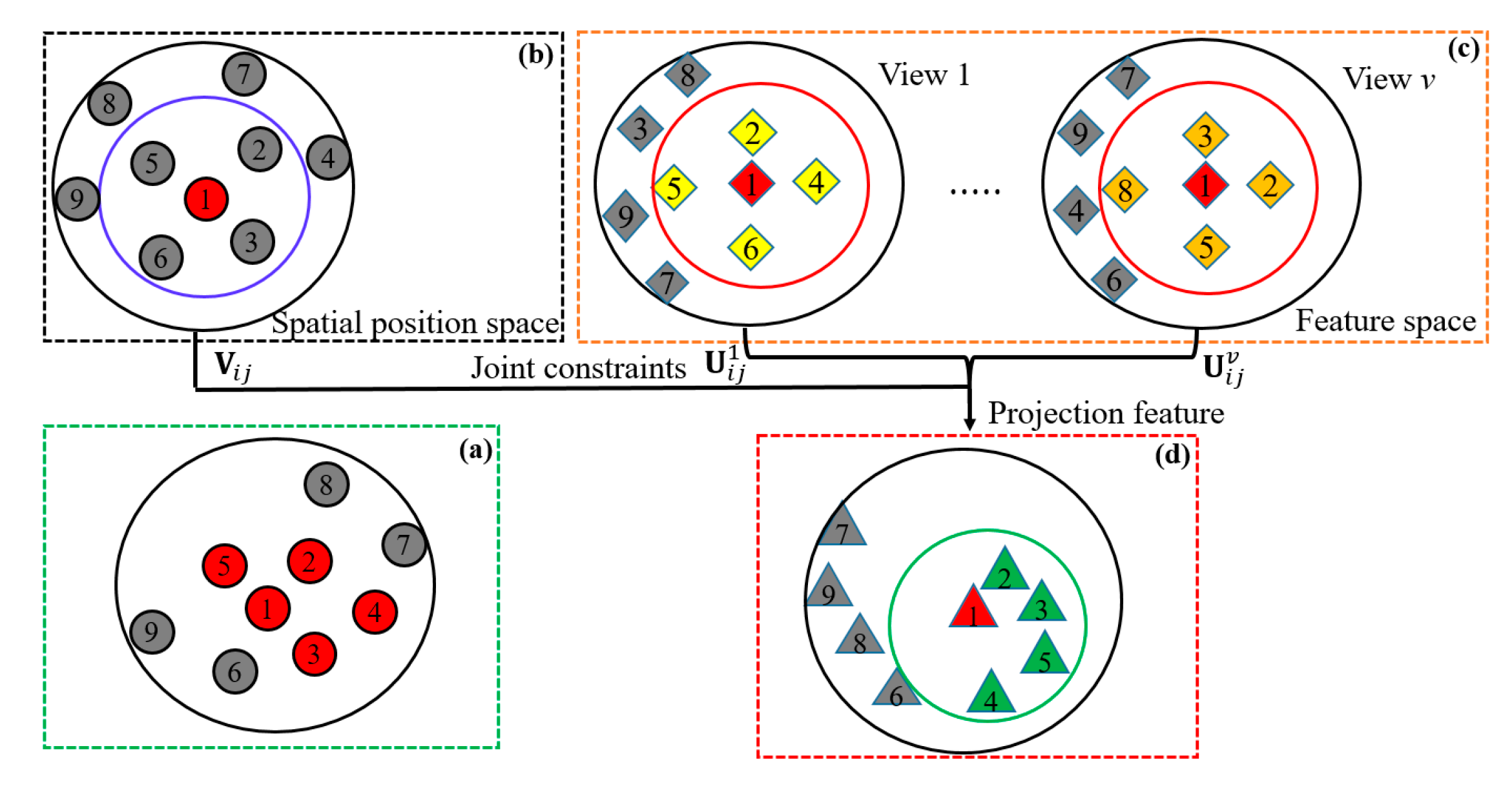
3.2.2. The Second Experimental Group

(1) Comparison methods

To evaluate the performance of our method, we compared results of nine related algorithms. To highlight the performance of the proposed multi-view features joint learning and fusion method, we compared it with three representative multi-view learning methods, i.e., adaptively weighted procrustes (AWP) [26], automatic multi-view graph and weights learning (AMGL) [23] and multi-view learning with adaptive neighbors (MLAN) [25]. AWP is an unsupervised method, which is compared with AMGL, MLAN and our method to show the performance of multi-view unsupervised and supervised classification methods. To prove the effectiveness of multi-view learning, we compared our method with non-negative sparse graph (NNSG) [19] and SVM [44]. Besides, we compare our method with FC_(our), FSI_(our), FC_(SVM) and FSI_(SVM) to show the effectiveness of multi-view features fusion. The compared algorithms and their recommended parameters are described below:

1) AWP 2018 [26]: a multi-view unsupervised classification algorithm based on adaptively weighted procrustes (AWP).

2) AMGL 2016 [23]: a new framework for automatic multi-view graph and weights learning. This method uses a small number of samples to train the classifier and further to predict unlabeled samples. In this paper, the neighborhood parameter of AMGL is set to 5, and the remaining parameters are assigned with default values of the source code that was released to the public in [23].

3) MLAN 2018 [25]: an effective multi-view model for adaptive learning of local data structure. The adaptive neighborhood value of MLAN is set to 9, and the remaining parameters are assigned with default parameters of the source codes in [25].

4) NNSG 2015 [19]: a non-negative sparse graph method for learning linear regression. We set ${\lambda }_1=0.001$, ${\lambda }_2=0.5$ and ${\lambda }_3=0.01$.

5) SVM [44]: multi-view features are directly concatenated together, which are then provided as input to SVM classifier for training and classification.

Apart from the comparisons with the above five methods, we also compared our results with FC_(our), FSI_(our), FC_(SVM) and FSI_(SVM) (see Section 3.2.1 for more detailed descriptions regarding these four configurations.)

(2) The results

For testing ALS point clouds, we randomly selected 9062 points from Scene2, from which 300 points (3.31%) were randomly selected for training. The remaining points were used as testing samples. Figure 6 shows a qualitative comparison result of the four multi-view methods. The quantitative comparison on all evaluation metrics are shown in

Table 8. Classification results of Scene2 (%). Precision/recall/intersection over union (IoU)/F₁-score, OA, mIoU, Kappa and mF₁ (%). Note that the highest accuracy values are highlighted in bold.

Method	Building	Car	Tree	OA	mIoU	Kappa	mF1
Our method	83.3/76.5 /66.3/79.8	29.9/67.1 /26.1/41.4	91.6/83.1 /77.2/87.2	79.7	56.6	64.3	69.4
AWP	69.2/78.6 /58.2/73.6	0.0/0.0 /0.0/0.0	84.4/84.3 /70.0/82.3	75.9	42.7	53.3	52
AMGL	81.9/70.3 /60.9/75.7	23.0//77.3 /21.5/35.5	95.1/77.4 /74.4/85.3	74.9	52.3	58.4	65.5
MLAN	48.7/100.0/ /48.7/65.5	0.0/0.0 /0.0/0.0	100.0/59.9 /59.9/74.9	64.8	36.2	41.4	46.8
NNSG	73.3/64.3 /52.1/68.5	12.0/87.9 /11.8/21.1	99.2/34.2 /34.1/50.9	48.4	32.7	30.5	46.8
SVM	84.6/66.7 /59.5/74.6	24.7/72.4/ /22.6/36.8	91.9/83.2 /77.5/87.3	76. 7	53.2	60	66.3
FC(our)	84.7/74.2 /65.5/79.1	27.1/65.4 /23.7/38.3	90.8/82.8 /76.4/86.6	78.6	55.2	62.7	68
FSI(our)	77.2/64.8 /54.3/70.5	22.8/59.8 /19.7/33.0	88.0/80.1 /72.2/83.9	73.4	48.8	53.8	62.5
FC(SVM)	83.8/65.4 /58.0/73.5	22.1/67.5 /20.0/33.3	90.1/80.7 /74.1/85.1	74.5	50.7	56.5	64
FSI(SVM)	81.3/55.8 /49.5/66.2	21.0/52.3 /17.6/30.0	84.5/86.0 /74.3/85.2	73.1	47.1	52	60.5

.

From the results listed in Table 8 and illustrated in Figure 6, we can make the following observations:

1) In Figure 6, the results of the proposed method and AMGL are closer to ground truth, the rest of qualitative results have relatively large errors. From Table 8, overall classification measures of 79.7%, 56.6%, 64.3% and 69.4% with regard to OA, mIoU, Kappa and mF₁ maintain the highest values, which demonstrates the advantages/superiority of the proposed method.

2) AWP has a high OA, but it cannot classify cars because the sample number of cars is relatively small in the experimental data. In addition, it is rare to see the categorized car points, as demonstrated in Figure 6c. In contrast, for AMGL algorithm, numerous tree points are mistakenly classified as cars (see Figure 6d). Although the classification precision of trees and the recall of buildings reached 100% using MLAN algorithm, numerous building points are misclassified as trees. In addition, the car points cannot be recognized, as demonstrated in Figure 6e. NNSG has capability to classify most cars, but a large number of building points and trees are falsely classified as cars, as evident in Figure 6f. The overall labeling results of NNSG is relatively poor. Although the SVM algorithm has the best classification performance of trees, the overall labeling results are inferior to ours.

3) For the covariance eigenvalues feature, the four overall evaluation metrics of the classification model obtained by our joint training method (FC_(our)) are at least 4% higher than the FC_(SVM). For the spin image feature, the classification results of our model trained by joint learning (FSI_(our)) also have certain advantages over FSI_(SVM). Therefore, we can make safe conclusions that the classification model jointly trained by our method is more effective than SVM-based model using single-view features. In addition, the classification performance of our multi-view fusion method outperforms the single-view feature classification.

For testing MLS point clouds, we randomly selected 12,000 points from Scene3 as experimental data, from which 1200 points (10%) were randomly selected for training. The remaining points are as testing samples. Figure 7 shows a qualitative comparison result of the multi-view methods. The quantitative comparison on all evaluation metrics are shown in

Table 9. Classification results of Scene3 (%). Precision/recall/IoU/F₁-score, OA, mIoU, Kappa and mF₁ (%). Note the highest accuracy values are highlighted in bold.

Method	Pole	Building	Car	Tree	OA	mIoU	Kappa	mF1
Our method	70.7/64.1 /50.7/67.3	62.1/70.1 /49.1/65.9	67.5/40.8 /34.1/50.9	68.3/92.9 /65.0/78.7	70	49.7	56	65.7
AWP	32.4/74.5 /29.2/45.2	0.0/0.0 /0.0/0.0	18.9/32.1 /13.5/23.8	0.0/0.0 /0.0/0.0	26.6	10.7	2.2	17.2
AMGL	31.1/22.4 /15.0/26.0	31.4/49.6 /23.8/38.5	31.0/16.9 /12.3/21.9	33.0/38.0 /21.5/35.3	31.7	18.1	9	30.4
MLAN	100.0/57.2 /57.2/72.8	69.2/57.8 /46.0/63.0	44.6/34.1 /24.0/38.7	60.3/100.0 /60.3/75.2	62.8	46.9	49.3	62.4
NNSG	53.7/49.1 /34.5/51.3	69.7/27.7 /24.8/39.6	74.1/13.0 /12.5/22.1	36.6/91.9 /35.4/52.4	45.5	26.8	27.3	41.4
SVM	63.0/66.0 /47.6/64.5	64.4/62.1 /46.2/63.2	61.1/46.7 /36.0/52.9	73.2/89.7 /67.6/80.6	66.1	49.3	54.8	65.3
FC(our)	54.5/59.1 /39.6/56.7	55.5/61.0 /41.0/58.1	56.3/30.8 /24.9/39.8	67.4/85.7 /60.6/75.5	65	47.8	53.3	64.1
FSI(our)	68.5/62.2 /48.4/65.2	60.6/68.7 /47.5/64.4	61.2/42.6 /33.5/50.2	68.4/86.4 /61.7/76.4	59.2	41.5	45.5	57.5
FC(SVM)	53.6/59.2 /39.2/56.3	57.3/55.9 /39.5/56.6	52.6/39.7 /29.2/45.3	69.8/81.3 /60.1/75.1	59	42	45.4	58.3
FSI(SVM)	66.4/60.6 /46.4/63.4	57.1/69.0 /45.5/62.5	56.3/36.0 /28.2/43.9	69.4/86.0 /62.3/76.8	62.9	45.6	50.5	61.7

.

From the results listed in Table 9 and illustrated in Figure 7, we can make the following observations:

1) In the qualitative and quantitative comparison, our method has better performance in the classification of point cloud in Scene3 than other methods. For the four classification evaluation metrics, our method has achieved the highest classification accuracy.

2) AWP, AMGL and NNSG have poor classification performances on each class of points, and there is a large number of misclassification points as demonstrated in Figure 7c–f. MLAN has the best overall classification result for the poles. Although this method has a highest recall value for tree classification, there are more misclassifications for the other class (see Figure 7e). SVM has the capability to distinguish trees and cars, achieving 36.0%/52.9% and 67.6%/80.6% with regard to IoU/F₁-score measures. Although the MLAN and SVM algorithms show the best labeling result for a certain class, we still have absolute advantages in terms of overall measure evaluations as we obtained 70.0%, 49.7%, 56.0% and 65.7% with regard to overall measures of OA, mIoU, Kappa and mF_1.

3) The classification results obtained by our multi-view fusion method are significantly improved compared with the single-view feature classification methods. In addition, the model of multi-view feature joint training and classification outperforms the multi-view feature direct fusion classification.

3.3. Effectiveness on ISPRS 3D Semantic Labeling Dataset

To prove the effectiveness of the proposed method for the International Society for Photogrammetry and Remote Sensing (ISPRS) 3D Semantic Labeling Dataset [45], we conducted an experiment on this dataset. Here, we add three kinds of features, i.e., fast-point feature histograms (FPFH), normal angle distribution histogram (NAD) and latitude sampling histogram (LSH) [3] as multi-view features. The experimental results are shown in Figure 8 and

Table 10. Classification results of ISPRS 3D Semantic Labeling Dataset (%). Precision/Recall/IoU/F1-score, OA, mIoU, Kappa and mF1 (%).

Metrics	Grounds	Cars	Buildings	Trees
Precision	91.4	92.1	93.4	85
Recall	94.2	48.3	87.3	90.8
F1-Score	92.8	63.4	90.2	87.8
OA	89.5
mIoU	73.3
Kappa	84.4
mF1	83.5

, which can demonstrate that the proposed method achieves a promising classification performance for the cars, trees, buildings and grounds.

3.4. Effectiveness of Multiple Constraints

In order to verify the contribution of each independent constraint (IC) in the objective function of our method, we compared the different ICs for point cloud classification. We use three configurations to prove the effectiveness of individual constraints:

(1) IC1: IC1 is the subspace learning term, which removes the redundant information by joint learning the multi-view feature transformation matrices and linear classifiers. Then the point cloud classification model can be obtained. The objective function is as follows:

$$\begin{array}{c}{\Theta }_{IC1}(H_v,W_v)=\arg \underset{H_v,W_v}{\min }{{\displaystyle \sum }}_{v=1}^m\parallel W_v{}^T{W}_v{X}_v-X_v{\parallel }_F^2+\alpha g(W_v{X}_v)\\ +{\lambda }_3(\parallel F-H_v{W}_v{X}_v{\parallel }_F^2+\gamma \parallel H_v{\parallel }_F^2)\end{array}$$

(21)

(2) IC2: Based on IC1, we introduce spatial position and feature space constraints into the objective function, as shown in Equation (22). The point cloud classification model is obtained by learning $H_v$ and $W_v$.

$$\begin{array}{l}{\Theta }_{IC2}(H_v,W_v)=\arg \underset{H_v,W_v}{\min }{{\displaystyle \sum }}_{v=1}^m\parallel W_v{}^T{W}_v{X}_v-X_v{\parallel }_F^2+\alpha g(W_v{X}_v)\\ \hspace{1em}\hspace{1em}\hspace{1em}\hspace{1em}\hspace{1em}\hspace{1em}+{\lambda }_{1}tr((W_v{X}_v)( L_{\mathrm{U}}^v+\beta L_V){(W_v{X}_v)}^T) +{\lambda }_3(\parallel F-H_v{W}_v{X}_v{\parallel }_F^2\\ \hspace{1em}\hspace{1em}\hspace{1em}\hspace{1em}\hspace{1em}\hspace{1em}+\gamma \parallel H_v{\parallel }_F^2)\end{array}$$

(22)

(3) IC3: In order to verify the contributions of multi-view joint training and multi-view classifier joint classification, we construct the classification model as shown in Equation (23), which directly concatenate the derived features of multi-views.

$$\begin{array}{c}{\Theta }_{\mathrm{IC}3}(H,W)=\arg \underset{H,W}{\min }\parallel W^{T}WX-X{\parallel }_F^2+\alpha g(WX)+{\lambda }_{1}tr((WX)(L_U+\beta L_V){(WX)}^T)\\ +{\lambda }_3(\parallel F-HWX{\parallel }_F^2+\gamma H{\parallel }_F^2)\end{array}$$

(23)

Here, to show the effectiveness of spatial position and feature space constraints, we compared IC1 with IC2. To show the advantages of multi-view learning, we compared our method and IC2 with IC3. Besides, we also compare our method with IC2 to prove the effectiveness of LCG. We arbitrarily select Scene1 (ALS point clouds with 3 classes) and Scene4 (MLS point clouds with 9 classes) to verify the effectiveness of individual constraints. In the experiment, 10,000 and 7200 points are selected from Scene1 and Scene4, respectively, which amounts to 0.8% points of testing sets. For IC1, IC2, IC3 and the proposed model, we keep the sum dimension number of the transformation features consistent (the sum dimension number of the new feature is 86), and the maximum iteration number is set to 20. The comparisons of the above three modified configurations with our classification results of each classification model are shown in

Table 11. Classification results of classification models with different configurations on Scene1 and Scene4 (%). Note the highest accuracy values are highlighted in bold.

Scene	Method	OA	mIoU	Kappa
Scene1 (ALS)	IC1	72.95	41.6	50.49
	IC2	74.46	43.32	53.42
	IC3	72.42	43.06	51.82
	Ours	77.49	45.04	57.15
Scene 4 (MLS)	IC1	79.29	29.35	66.37
	IC2	80.68	30.86	68.3
	IC3	79.39	31.38	67.05
	Ours	80.93	30.92	68.62

.

From Table 11, we have the following observations.

(1) IC2 outperforms IC1. The main reason is that the consistency constraint of position and feature spaces is introduced in different views, so the learned subspace can better reflect the local geometry of the data and the consistency of the local space distribution among different views.

(2) Our method achieves 77.49%/80.93% and 57.15%/68.62% with regarding to OA and Kappa measures on Scene1/Scene4, which are 4.54%/1.64% and 6.66%/1.25% higher than IC1, and 3.03%/0.25% and 3.73%/0.32% higher than IC2. The experimental results prove that the constraints of LCG and label consistency among different views are effective. The joint learning of the feature transformation matrix and classifier can effectively improve the accuracy of point cloud classification. The main reason is that LCG makes the learned subspace more discriminative, and the constraints among different views make the trend of the feature expression and classification results of different views more consistent.

(3) The overall performance of our method outperforms IC3. The experimental results show that the multi-view joint learning classification method for features projecting and fusion is more effective than the direct fusion classification methods. The main reason is that different features reflect the different attributes of the same point. The features of multi-view can make full use of the attributes of each point through joint constraint, which can achieve better classification results than the method of multiple features direct fusion.

3.5. Parameters Analysis

In the proposed method, there are mainly 7 key parameters that need to be tuned, including $\alpha ,\beta , \gamma ,\delta ,{\lambda }_1,{\lambda }_2$ and ${\lambda }_3$. In the experiment, we set α = 0.1, β =0.01, and δ =0.001.

Parameters of ${\lambda }_1$, ${\lambda }_2$ and ${\lambda }_3$ correspond to the terms of position space and feature space constraint, multi-view LCG constraint and multi-view LCS constraint, respectively. We jointly discuss ${\lambda }_2$ and ${\lambda }_3$, which affect the weight of the LCG term and LCS term. Figure 9a,b show the classification accuracy of different ${\lambda }_2$ and ${\lambda }_3$ on Scene1 and Scene4 when ${\lambda }_1$ is fixed. It can be seen that the difference of accuracy with different ${\lambda }_2$ and ${\lambda }_3$ is small, which is within 0.8% and 0.05% for Scene1 and Scene4, respectively. This demonstrates that ${\lambda }_2$ and ${\lambda }_3$ have a small influence on the classification result when they vary within the given values. Moreover, the accuracy fluctuations are smooth, i.e., the classification accuracy is relatively less affected by the varying ${\lambda }_2$ and ${\lambda }_3$ when ${\lambda }_1$ is fixed. In addition, as shown in Figure 9c,d, when ${\lambda }_3$ is fixed, and ${\lambda }_1$ and ${\lambda }_2$ varies within given ranges, the classification accuracy of our method on different parameter values has larger changes, which is within 5.5% and 0.25% for Scene1 and Scene4, respectively. However, the accuracy fluctuation caused by the change of ${\lambda }_1$ and ${\lambda }_2$ (fixed ${\lambda }_1$) is relatively stable, except for some values of parameters. As shown in Figure 9e,f, when ${\lambda }_2$ is fixed, and ${\lambda }_1$ and ${\lambda }_3$ varies within given values, and the classification accuracy difference of our method on different parameter values is within 2.5% and 0.2% for Scene1 and Scene4, respectively. Besides, we can also find that the accuracy fluctuations are relatively small, i.e., the proposed method is relatively stable, which has less influence by the varying ${\lambda }_1$ and ${\lambda }_3$ when ${\lambda }_2$ is fixed. From Figure 9, we can observe that the accuracy fluctuation trends of the two scenes are similar for each situation (two parameter values vary when a parameter value fixes). Besides, the comparisons of these three situations demonstrate that ${\lambda }_1$ has the largest influence on classification accuracy, and ${\lambda }_2$ and ${\lambda }_3$ have relatively small influence on classification accuracy. From the above analysis we can draw a safe conclusion that the parameters of our method have a low impact on the point cloud classification in a certain range. That is, our method is relatively insensitive to parameters ${\lambda }_1$, ${\lambda }_2$ and ${\lambda }_3$.

3.6. Convergence Analysis

The objective function shown in Equation (11) is highly non-linear, although it is solvable, it is very difficult to simultaneously optimize the variables $W_v$, $G_v$ and $H_v$. Figure 10 reports the objective function values within the 25 iterations. The objective function is optimized by the proposed update rules depicted in Algorithm 1. Figure 10a,b are the objective function value curves corresponding to Scene1 and Scene4. We can see that our optimization method can quickly converge to a local or even global minimum for our two scenes.

4. Conclusions

In this paper, we have proposed a multi-view joint learning framework for point cloud classification, which includes multi-view subspace learning term for removing redundant information and representing low-dimensional features; the local distribution consistency constraint of feature space and position space term for the adjacency expression of neighborhood points; and the label consistency terms with the consistency between the predicted labels of all views and the ground truth label and the consistency among the predicted labels of each view. These terms are joined to learn the transformation matrices and optimal classifiers by the iterative optimization algorithm of objective function, and the convergence is very fast. Experiments performed on two ALS point cloud scenes, two MLS point cloud scenes and a TLS point cloud scene with fewer training points clearly confirm that our method outperforms the compared algorithms. Although our method achieves more promising classification accuracy than the compared algorithms, there are some drawbacks and interesting ideas that can be further explored to extend the research reported in this paper. Currently, the proposed method cannot achieve accurate semantic labeling of city-level point clouds having complex geometric shapes and diverse objects. In addition, the derived multiple features are relatively simple. Point set features and high-level features are not fully explored. In future work, the multi-view joint learning method and deep-learning technologies can be combined to learn a multi-view deep-learning network for improving the semantic labeling of point clouds.

References

1. Zhang, Z.; Zhang, L.; Tong, X. Discriminative-dictionary-learning-based multilevel point-cluster features for ALS point-cloud classification. IEEE Trans. Geosci. Remote Sens. 2016, 54, 7309–7322. [Google Scholar] [CrossRef]
2. Farabet, C.; Couprie, C.; Najman, L. Learning hierarchical features for scene labeling. IEEE Trans. Pattern Anal. Mach. Intell. 2012, 35, 1915–1929. [Google Scholar] [CrossRef] [Green Version]
3. Li, Y.; Tong, G.; Du, X. A single point-based multilevel features fusion and pyramid neighborhood optimization method for ALS point cloud classification. Appl. Sci. 2019, 9, 951. [Google Scholar] [CrossRef] [Green Version]
4. Li, Y.; Tong, G.; Li, X. MVF-CNN: Fusion of multilevel features for large-scale point cloud classification. IEEE Access. 2019, 7, 46522–46537. [Google Scholar] [CrossRef]
5. Wang, Z.; Zhang, L.; Fang, T. A multiscale and hierarchical feature extraction method for terrestrial laser scanning point cloud classification. IEEE Trans. Geosci. Remote Sens. 2014, 53, 2409–2425. [Google Scholar] [CrossRef]
6. Guo, B.; Huang, X.; Zhang, F. Classification of airborne laser scanning data using JointBoost. ISPRS J. Photogramm. Remote Sens. 2015, 100, 71–83. [Google Scholar] [CrossRef]
7. Weinmann, M.; Jutzi, B.; Hinz, S. Semantic point cloud interpretation based on optimal neighborhoods, relevant features and efficient classifiers. ISPRS J. Photogramm. Remote Sens. 2015, 105, 286–304. [Google Scholar] [CrossRef]
8. Chen, D.; Peethambaran, J.; Zhang, Z. A supervoxel-based vegetation classification via decomposition and modelling of full-waveform airborne laser scanning data. Int. J. Remote Sens. 2018, 39, 2937–2968. [Google Scholar] [CrossRef]
9. Li, Y.; Chen, D.; Du, X. Higher-order conditional random fields-based 3D semantic labeling of airborne laser-scanning point clouds. Remote Sens. 2019, 11, 1248. [Google Scholar] [CrossRef] [Green Version]
10. Zhang, Q.; Li, B. Discriminative K-SVD for dictionary learning in face recognition. In Proceedings of the IEEE Computer Society Conference on Computer Vision and Pattern Recognition, San Francisco, CA, USA, 13–18 June 2010. [Google Scholar]
11. Aharon, M.; Elad, M.; Bruckstein, A. K-SVD: An algorithm for designing overcomplete dictionaries for sparse representation. IEEE Trans. Signal Process. 2006, 54, 4311–4322. [Google Scholar] [CrossRef]
12. Jiang, Z.; Lin, Z.; Davis, L. Label consistent K-SVD: Learning a discriminative dictionary for recognition. IEEE Trans. Pattern Anal. Mach. Intell. 2013, 35, 2651–2664. [Google Scholar] [CrossRef] [PubMed]
13. Mei, J.; Wang, Y.; Zhang, L. PSASL: Pixel-level and superpixel-level aware subspace learning for hyperspectral image classification. IEEE Trans. Geosci. Remote Sens. 2019, 57, 4278–4293. [Google Scholar] [CrossRef]
14. Le, Q.; Karpenko, A.; Ngiam, J. ICA with reconstruction cost for efficient overcomplete feature learning. In Proceedings of the Advances in Neural Information Processing Systems, Granada, Spain, 12–14 December 2011. [Google Scholar]
15. Martínez, A.; Kak, A. PCA versus LDA. IEEE Trans. Pattern Anal. Mach. Intell. 2001, 23, 228–233. [Google Scholar] [CrossRef] [Green Version]
16. Nie, F.; Yuan, J.; Huang, H. Optimal mean robust principal component analysis. In Proceedings of the International Conference on Machine Learning, Beijing, China, 21–26 June 2014. [Google Scholar]
17. Mei, J.; Zhang, L.; Wang, Y. Joint margin, cograph, and label constraints for semisupervised scene parsing from point clouds. IEEE Trans. Geosci. Remote Sens. 2018, 56, 3800–3813. [Google Scholar] [CrossRef]
18. Zhu, P.; Zhang, L.; Wang, Y. Projection learning with local and global consistency constraints for scene classification. ISPRS J. Photogramm. Remote Sens. 2018, 144, 202–216. [Google Scholar] [CrossRef]
19. Fang, X.; Xu, Y.; Li, X. Learning a nonnegative sparse graph for linear regression. IEEE Trans. Image Process. 2015, 24, 2760–2771. [Google Scholar] [CrossRef]
20. Johnson, A. A Representation for 3D Surface Matching. Ph.D. Thesis, Robotics Institute, Carnegie Mellon University, Pittsburgh, PA, USA, 1997. [Google Scholar]
21. Rusu, R.; Blodow, N.; Beetz, M. Fast point feature histograms (FPFH) for 3D registration. In Proceedings of the IEEE International Conference on Robotics and Automation, Kobe, Japan, 12–17 May 2009. [Google Scholar]
22. Rusu, R.; Bradski, G.; Thibaux, R. Fast 3D recognition and pose using the Viewpoint Feature Histogram. In Proceedings of the IEEE/RSJ International Conference on Intelligent Robots and Systems, Taipei, Taiwan, 18–22 October 2010. [Google Scholar]
23. Nie, F.; Li, J.; Li, X. Parameter-free auto-weighted multiple graph learning: A framework for multiview clustering and semi-supervised classification. In Proceedings of the International Joint Conference on Artificial Intelligence, New York, NY, USA, 9–15 July 2016. [Google Scholar]
24. Nie, F.; Cai, G.; Li, X. Multi-view clustering and semi-supervised classification with adaptive neighbours. In Proceedings of the AAAI Conference on Artificial Intelligence, San Francisco, CA, USA, 4–9 February 2017. [Google Scholar]
25. Nie, F.; Cai, G.; Li, J. Auto-weighted multi-view learning for image clustering and semi-supervised classification. IEEE Trans. Image Process. 2018, 27, 1501–1511. [Google Scholar] [CrossRef]
26. Nie, F.; Tian, L.; Li, X. Multiview clustering via adaptively weighted procrustes. In Proceedings of the ACM SIGKDD International Conference on Knowledge Discovery and Data Mining, London, UK, 19–23 August 2018. [Google Scholar]
27. Zhang, C.; Hu, Q.; Fu, H. Latent multi-view subspace clustering. In Proceedings of the IEEE Conference on Computer Vision and Pattern Recognition, Honolulu, HI, USA, 21–26 July 2017. [Google Scholar]
28. Wang, X.; Guo, X.; Lei, Z. Exclusivity-consistency regularized multi-view subspace clustering. In Proceedings of the IEEE Conference on Computer Vision and Pattern Recognition, Honolulu, HI, USA, 21–26 July 2017. [Google Scholar]
29. Cao, X.; Zhang, C.; Fu, H. Diversity-induced multi-view subspace clustering. In Proceedings of the IEEE Conference on Computer Vision and Pattern Recognition, Boston, MA, USA, 7–12 June 2015. [Google Scholar]
30. Wang, Y.; Wu, L.; Lin, X. Multiview spectral clustering via structured low-rank matrix factorization. IEEE Trans. Neural Netw. Learn. Syst. 2018, 29, 4833–4843. [Google Scholar] [CrossRef] [Green Version]
31. Tang, C.; Zhu, X.; Liu, X. Learning joint affinity graph for multi-view subspace clustering. IEEE Trans. Multimedia 2019, 21, 1724–1736. [Google Scholar] [CrossRef]
32. Griffiths, D.; Boehm, J. A Review on deep learning techniques for 3D sensed data classification. Remote Sens. 2019, 11, 1499. [Google Scholar] [CrossRef] [Green Version]
33. Su, H.; Maji, S.; Kalogerakis, E.; Learned-Miller, E. Multi-view convolutional neural networks for 3D shape recognition. In Proceedings of the IEEE International Conference on Computer Vision (ICCV), Santiago, Chile, 7–13 December 2015. [Google Scholar]
34. Boulch, A.; Guerry, J.; Le Saux, B.; Audebert, N. SnapNet: 3D point cloud semantic labeling with 2D deep segmentation networks. Comput. Graph. 2018, 71, 189–198. [Google Scholar] [CrossRef]
35. Felix, J.; Martin, D.; Patrik, T.; Goutam, B.; Fahad, S.; Michael, F. Deep projective 3D semantic segmentation. In International Conference on Computer Analysis of Images and Patterns; Lecture Notes in Computer Science Series Volume 10424; Springer: Cham, Switzerland, 2017; pp. 95–107. [Google Scholar]
36. Qin, N.; Hu, X.; Dai, H. Deep fusion of multi-view and multimodal representation of ALS point cloud for 3D terrain scene recognition. ISPRS J. Photogramm. Remote Sens. 2018, 143, 205–212. [Google Scholar] [CrossRef]
37. Ronneberger, O.; Fischer, P.; Brox, T. U-Net: Convolutional networks for biomedical image segmentation. In International Conference on Medical Image Computing and Computer-Assisted Intervention; Lecture Notes in Computer Science Series Volume 9351; Springer International Publishing: Cham, Switzerland, 2015; pp. 234–241. [Google Scholar]
38. Badrinarayanan, V.; Kendall, A.; Cipolla, R. SegNet: A deep convolutional encoder-decoder architecture for image segmentation. IEEE Trans. Pattern Anal. Mach. Intell. 2015, 39, 2481–2495. [Google Scholar] [CrossRef]
39. Shelhamer, E.; Long, J.; Darrell, T. Fully convolutional networks for semantic segmentation. IEEE Trans. Pattern Anal. Mach. Intell. 2017, 39, 640–651. [Google Scholar] [CrossRef] [PubMed]
40. Malouf, R. A comparison of algorithms for maximum entropy parameter estimation. In Proceedings of the 6th Conference on Computational Natural Language Learning CoNLL 2002, Taipei, Taiwan, 31 August–1 September 2002. [Google Scholar]
41. Zhang, Z.; Zhang, L.; Tong, X.; Mathiopoulos, P.; Guo, B.; Huang, X.; Wang, Z.; Wang, Y. A multilevel point-cluster-based discriminative feature for ALS point cloud classification. IEEE Trans. Geosci. Remote Sens. 2016, 54, 3309–3321. [Google Scholar] [CrossRef]
42. Huang, H.; Wang, L.; Jiang, B. Precision verification of 3D SLAM backpacked mobile mapping robot. Bull. Surv. Mapp. 2016, 12, 68–73. [Google Scholar]
43. Tong, G.; Li, Y.; Zhang, W.; Chen, D.; Zhang, Z.; Yang, J.; Zhang, J. Point set multi-level aggregation feature extraction based on multi-scale max pooling and LDA for point cloud classification. Remote Sens. 2019, 11, 2846. [Google Scholar] [CrossRef] [Green Version]
44. Chang, C.; Lin, C. LIBSVM: A library for support vector machines. ACM Trans. Intell. Syst. Technol. 2011, 2, 27. [Google Scholar] [CrossRef]
45. Niemeyer, J.; Rottensteiner, F.; Sörgel, U. Contextual classification of lidar data and building object detection in urban areas. ISPRS J. Photogramm. Remote Sens. 2014, 87, 152–165. [Google Scholar] [CrossRef]
Figure 1. The flowchart of the proposed method. (a) Training data; (b) testing data, (c) feature extraction; (d) the process of multiple views and space representation consistency under constraints of label consistency (MvsRCLC); (e) classification results. X1 and Xv represent the first view and the vth view features of the point cloud, respectively.
Remotesensing 12 00135 g001
Figure 2. The schematic diagram of feature space and spatial position space joint constraints. (a) ground truth, (b) 5 neighbor points of p1 in spatial position space, (c) 5 neighbor points of point p1 for different view features in feature space, (d) the projection results (subspace features) with the joint constraints of spatial position space and feature space. Note that different numbers represent different point clouds. Different colors represent different classes. The red point labeled 1 is the selected point p1.
Remotesensing 12 00135 g002
Figure 3. Five different point cloud scenes used in this paper. Subfigures from (a) to (e) represent the scanned Scene1 to Scene5.
Remotesensing 12 00135 g003aRemotesensing 12 00135 g003bRemotesensing 12 00135 g003c
Figure 4. Classification results of Scene2. (a) Ground truth; (b) our method; (c) RICA-SVM.
Remotesensing 12 00135 g004
Figure 5. Classification results of Scene4. (a) Ground truth; (b) our method; (c) LCKSVD1; (d) LCKSVD2; (e) DKSVD; (f) RICA-SVM.
Remotesensing 12 00135 g005aRemotesensing 12 00135 g005b
Figure 6. Classification results of ALS point clouds selected from Scene2. (a) Ground truth; (b) our method; (c) AWP; (d) AMGL; (e) MLAN; (f) NNSG.
Remotesensing 12 00135 g006
Figure 7. Classification results of MLS point cloud selected from Scene3. (a) Ground truth; (b) our method; (c) AWP; (d) AMGL; (e) MLAN; (f) NNSG. Note that our method obviously outperforms other methods in black box regions.
Remotesensing 12 00135 g007
Figure 8. Classification results on ISPRS 3D Semantic Labeling Dataset.
Remotesensing 12 00135 g008
Figure 9. The influence of different parameters on the classification accuracy. (a,b) are the classification accuracy corresponding to different λ 2 and λ 3 in Scene1 and Scene4 when λ 1 is fixed, respectively. (c,d) are the classification accuracy corresponding to different λ 1 and λ 2 in Scene1 and Scene4 when λ 3 is fixed, respectively. (e,f) are the classification accuracy corresponding to different λ 1 and λ 3 in Scene1 and Scene4 when λ 2 is fixed, respectively.
Remotesensing 12 00135 g009
Figure 10. Convergence processes for Scene1 and Scene4 in subfigure (a,b).
Remotesensing 12 00135 g010