Deriving Regional Snow Line Dynamics during the Ablation Seasons 1984–2018 in European Mountains

Abstract

1. Introduction
2. Data and Study Areas
2.1. Satellite Data and Pre-Processing
2.2. Auxiliary Data
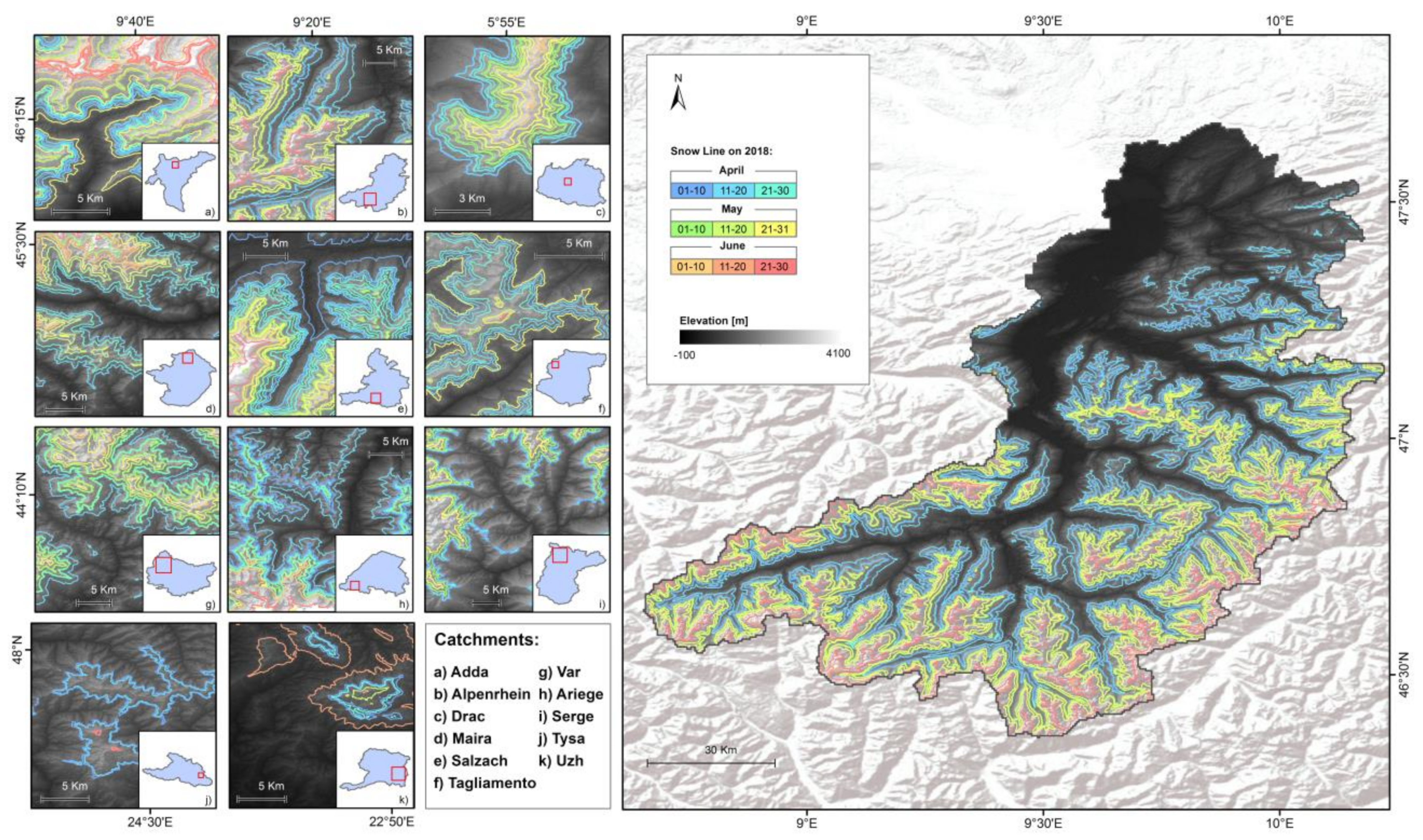
2.3. Study Areas
3. Methods
3.1. Snow Cover Classification and Validation
- Snow classification: In this study, the algorithms developed by Klein et al. [32] and Poon and Valeo [33] is employed to classify snow. The algorithm is based on a decision tree with multiple thresholds on the normalized difference snow index (NDSI), the green band, and the near infra-red (NIR) band. To detect snow in forested areas, the NDSI-NDVI (normalized difference vegetation index) field is utilized to calibrate the snow cover classification results therein.
- Cloud mask: Three different types of cloud masks are applied because of different designations of Landsat, ASTER, and Sentinel-2. Firstly, the Mountainous Fmask (MFmask) [34,35,36,37] is deployed to mask out the clouds in Landsat scenes. Secondly, “s2cloudless” is employed to exclude the clouds in Sentinel-2 images, which is an automated single-scene pixel-based cloud detector developed by the Sentinel Hub’s research team (available on GitHub: https://github.com/sentinel-hub/sentinel2-cloud-detector, accessed on 06 March 2019). Thirdly, the automatic cloud cover assessment (ACCA) [38,39] is applied to identify the clouds in ASTER scenes.
- Water mask: High NDSI values usually indicate the presence of the snow in optical EO imagery. However, such high NDSI values could also be observed in clear water bodies. Therefore, water bodies must be masked out to avoid misclassification. Because the water bodies commonly show positive normalized difference water index (NDWI) values, and the reflectance of water bodies in the green band is relatively low, the water mask is generated based on thresholding these two values.
- Shadow mask: Shadow-cast areas are normally treated as non-valid pixels. In this study, the shadow pixels are identified following the methods from the ESA satellite snow product intercomparison and evaluation exercise (SnowPEX) Team [40]. Thereafter, the shadow-cast pixels are masked out in the snow cover results.
- Thermal mask: Both Landsat and ASTER have thermal bands. To filter out bright and warm surfaces such as warm rocks in the classification results, a thermal threshold (<288 K) introduced by Metsämäki et al. [41] is applied to Landsat- and ASTER-based snow classifications. Sentinel-2 does not have any thermal band, which could potentially commit more commission errors over bright and warm targets.
3.2. Regional Snow Line Elevation Retrieval and Accuracy Assessment
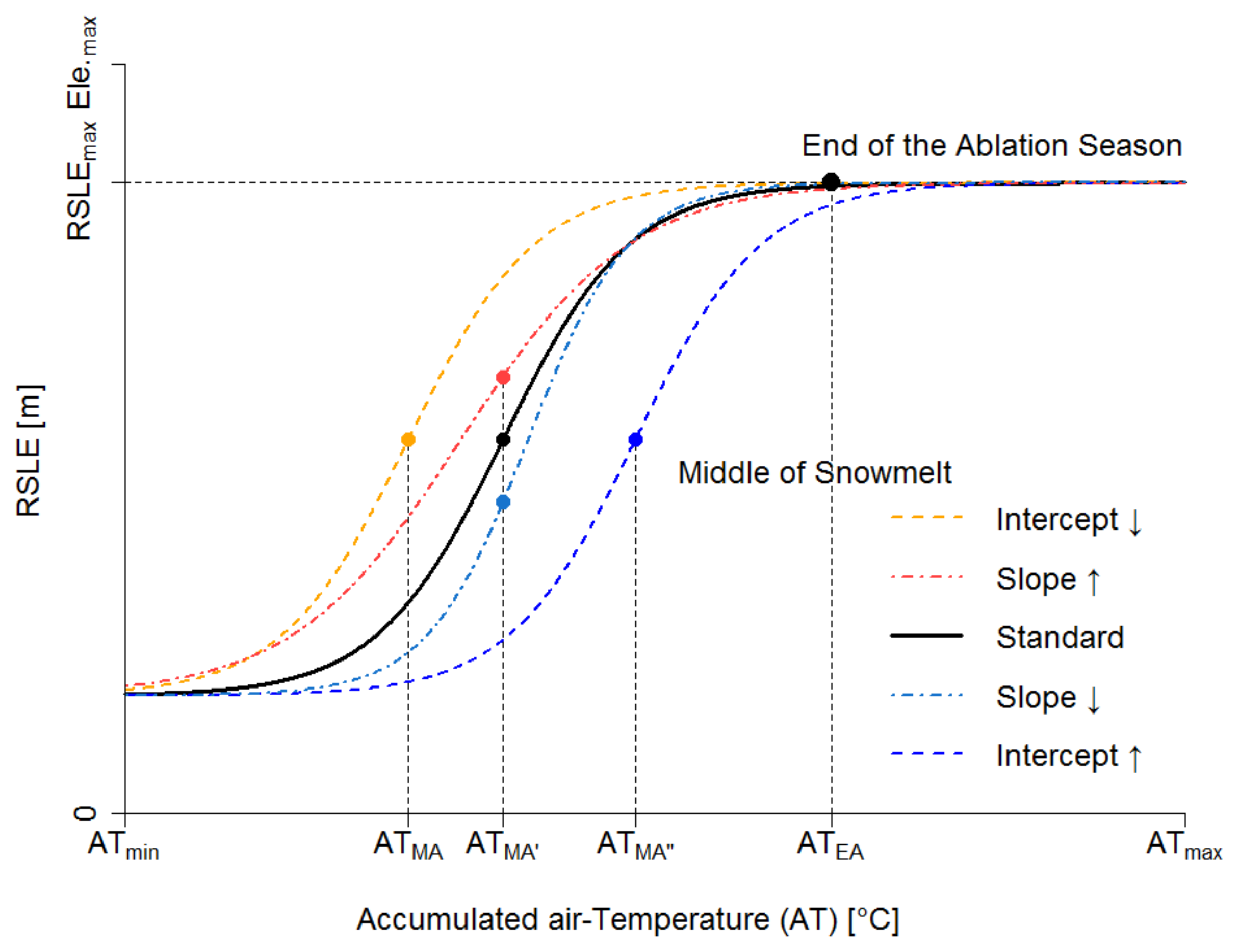
3.3. Regional Snow Line Retreat Curve (RSLRC) Derivation and Validation
4. Results
4.1. Intra-Annual Variations of Regional Snow Lines during the Ablation Season 2018
4.2. Inter-Annual Variations of Regional Snow Lines during the Ablation Seasons 1984–2018
4.3. Accuracy Assessment
4.3.1. Accuracy Assessment of the Snow Classification Results
4.3.2. Accuracy Assessment of the Regional Snow Line Elevations (RSLEs)
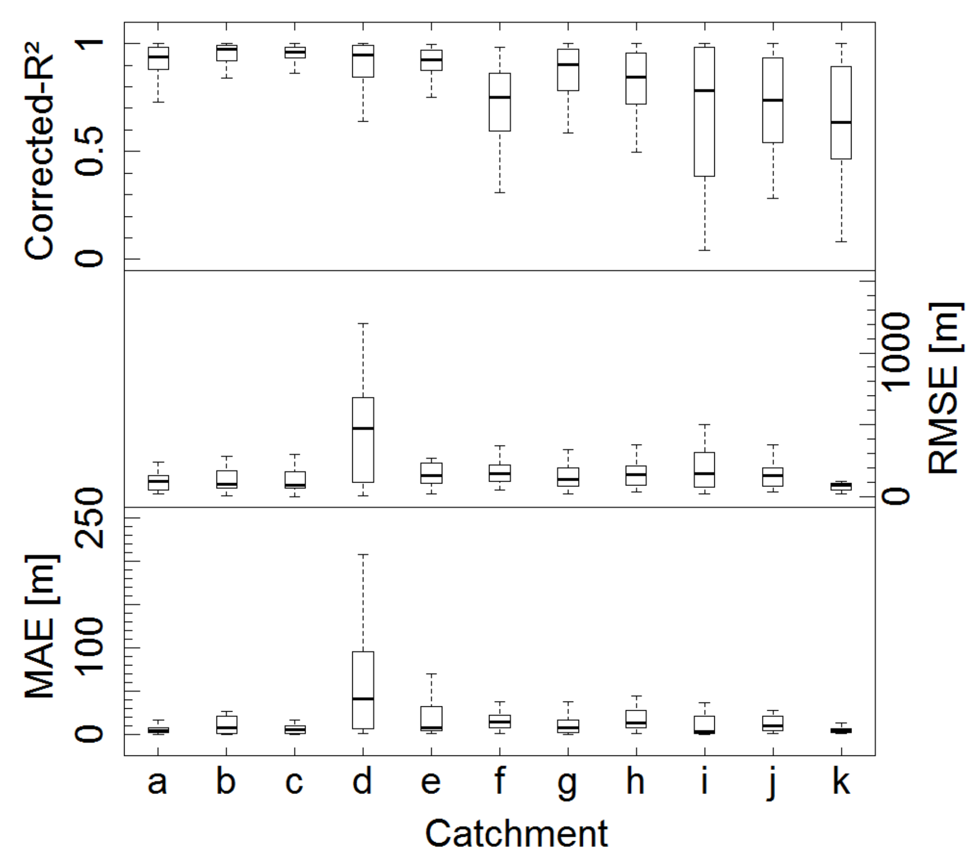
4.3.3. Accuracy Assessment of the Regional Snow Line Retreat Curves (RSLRCs)
5. Discussion
5.1. Challenges in Accurately Deriving Regional Snow Line Elevations (RSLEs) and Regional Snow Line Retreat Curves (RSLRCs)
5.2. Challenges of Validation
5.3. Observed Regional Snow Lines Dynamics
6. Summary and Conclusions
Author Contributions
Funding
Acknowledgments
Conflicts of Interest
References
- Derksen, C.; Brown, R. Spring snow cover extent reductions in the 2008–2012 period exceeding climate model projections. Geophys. Res. Lett. 2012, 39. [Google Scholar] [CrossRef]
- Mudryk, L.R.; Kushner, P.J.; Derksen, C.; Thackeray, C. Snow cover response to temperature in observational and climate model ensembles. Geophys. Res. Lett. 2017, 44, 919–926. [Google Scholar] [CrossRef]
- Metsämäki, S.; Böttcher, K.; Pulliainen, J.; Luojus, K.; Cohen, J.; Takala, M.; Mattila, O.-P.; Schwaizer, G.; Derksen, C.; Koponen, S. The accuracy of snow melt-off day derived from optical and microwave radiometer data—A study for Europe. Remote Sens. Environ. 2018, 211, 1–12. [Google Scholar] [CrossRef]
- Hoegh-Guldberg, O.; Jacob, D.; Taylor, M.; Bindi, M.; Brown, S.; Camilloni, I.; Diedhiou, A.; Djalante, R.; Ebi, K.; Engelbrecht, F.; et al. Impacts of 1.5 °C global warming on natural and human systems. Available online: https://www.ipcc.ch/sr15/ (accessed on 16 April 2019).
- IPCC. Climate Change 2013: The Physical Science Basis: Working Group I Contribution to the Fifth Assessment Report of the Intergovernmental Panel on Climate Change; Cambridge University Press: Cambridge, UK, 2013. [Google Scholar]
- IPCC. Climate Change 2014: Impacts, Adaptation, and Vulnerability-Part B: Regional Aspects-Contribution of Working Group II to the Fifth Assessment Report of the Intergovernmental Panel on Climate Change; Cambridge University Press: Cambridge, UK, 2014. [Google Scholar]
- EC White Paper-Adapting to Climate Change: Towards a European Framework for Action. Available online: https://ec.europa.eu/health/ph_threats/climate/docs/com_2009_147_en.pdf (accessed on 6 March 2019).
- Barnett, T.P.; Adam, J.C.; Lettenmaier, D.P. Potential impacts of a warming climate on water availability in snow-dominated regions. Nature 2005, 438, 303–309. [Google Scholar] [CrossRef] [PubMed]
- Jennings, K.S.; Winchell, T.S.; Livneh, B.; Molotch, N.P. Spatial variation of the rain—Snow temperature threshold across the Northern Hemisphere. Nat. Commun. 2018, 9, 1148. [Google Scholar] [CrossRef]
- Hu, Z.; Kuenzer, C.; Dietz, A.J.; Dech, S. The Potential of Earth Observation for the Analysis of Cold Region Land Surface Dynamics in Europe—A Review. Remote Sens. 2017, 9, 1067. [Google Scholar] [CrossRef]
- Tekeli, A.E.; Akyürek, Z.; Şorman, A.A.; Şensoy, A.; Şorman, A.Ü. Using MODIS snow cover maps in modeling snowmelt runoff process in the eastern part of Turkey. Remote Sens. Environ. 2005, 97, 216–230. [Google Scholar] [CrossRef]
- Dietz, A.J.; Wohner, C.; Kuenzer, C. European snow cover characteristics between 2000 and 2011 derived from improved MODIS daily snow cover products. Remote Sens. 2012, 4, 2432–2454. [Google Scholar] [CrossRef]
- Hu, Z.; Dietz, A.; Kuenzer, C. The potential of retrieving snow line dynamics from Landsat during the end of the ablation seasons between 1982 and 2017 in European mountains. Int. J. Appl. Earth Obs. Geoinf. 2019, 78, 138–148. [Google Scholar] [CrossRef]
- Parajka, J.; Bezak, N.; Burkhart, J.; Hauksson, B.; Holko, L.; Hundecha, Y.; Jenicek, M.; Krajčí, P.; Mangini, W.; Molnar, P.; et al. MODIS snowline elevation changes during snowmelt runoff events in Europe. J. Hydrol. Hydromech. 2019, 67, 101–109. [Google Scholar] [CrossRef]
- Krajčí, P.; Holko, L.; Perdigão, R.A.P.; Parajka, J. Estimation of regional snowline elevation (RSLE) from MODIS images for seasonally snow covered mountain basins. J. Hydrol. 2014, 519, 1769–1778. [Google Scholar] [CrossRef]
- Takala, M.; Pulliainen, J.; Metsamaki, S.J.; Koskinen, J.T. Detection of snowmelt using spaceborne microwave radiometer data in Eurasia from 1979 to 2007. IEEE Trans. Geosci. Remote Sens. 2009, 47, 2996–3007. [Google Scholar] [CrossRef]
- Klein, G.; Vitasse, Y.; Rixen, C.; Marty, C.; Rebetez, M. Shorter snow cover duration since 1970 in the Swiss Alps due to earlier snowmelt more than to later snow onset. Clim. Change 2016, 139, 637–649. [Google Scholar] [CrossRef]
- Hüsler, F.; Jonas, T.; Riffler, M.; Musial, J.P. A satellite-based snow cover climatology (1985–2011) for the European Alps derived from AVHRR data. Cryosphere 2014, 8, 73. [Google Scholar] [CrossRef]
- Macander, M.J.; Swingley, C.S.; Joly, K.; Raynolds, M.K. Landsat-based snow persistence map for northwest Alaska. Remote Sens. Environ. 2015, 163, 23–31. [Google Scholar] [CrossRef]
- Wayand, N.E.; Marsh, C.B.; Shea, J.M.; Pomeroy, J.W. Globally scalable alpine snow metrics. Remote Sens. Environ. 2018, 213, 61–72. [Google Scholar] [CrossRef]
- Leaf, C.F. Areal extent of snow cover in relation to streamflow in Central Colorado. In Proceedings of the International Hydrology Symposium, Fort Collins, CO, USA, 6–8 September 1967; Volume 1, pp. 157–164. [Google Scholar]
- Hall, D. Remote Sensing of Ice and Snow; Springer Science & Business Media: London, UK, 2012. [Google Scholar]
- Rango, A.; Martinec, J. Application of a snowmelt-runoff model using Landsat data. Hydrol. Res. 1979, 10, 225–238. [Google Scholar] [CrossRef]
- Martinec, J. Snowmelt-runoff model for stream flow forecasts. Hydrol. Res. 1975, 6, 145–154. [Google Scholar] [CrossRef]
- WMO. The Role of Climatological Normals in a Changing Climate. Available online: https://library.wmo.int/doc_num.php?explnum_id=4546 (accessed on 6 March 2019).
- GCOS. The Global Observing System for Climate: Implementation Needs. Available online: https://unfccc.int/sites/default/files/gcos_ip_10oct2016.pdf (accessed on 6 March 2019).
- Wulder, M.A.; Masek, J.G.; Cohen, W.B.; Loveland, T.R.; Woodcock, C.E. Opening the archive: How free data has enabled the science and monitoring promise of Landsat. Remote Sens. Environ. 2012, 122, 2–10. [Google Scholar] [CrossRef]
- Rango, A.; Martinec, J. Snow accumulation derived from modified depletion curves of snow coverage. In Proceedings of the Exeter Symposium, Hydrological Aspects of Alpine and High Mountain Areas, Exeter, UK, 19–30 July 1982; Volume 138, pp. 83–89. [Google Scholar]
- Richter, R.; Schläpfer, D. Atmospheric/topographic correction for satellite imagery: ATCOR-2/3 User Guide. DLR IB 2011, 2011, 501–565. [Google Scholar]
- Tachikawa, T.; Hato, M.; Kaku, M.; Iwasaki, A. Characteristics of ASTER GDEM version 2. In Proceedings of the 2011 IEEE International Geoscience and Remote Sensing Symposium, Vancouver, BC, Canada, 24–29 July 2011. [Google Scholar]
- Berrisford, P.; Dee, D.; Fielding, K.; Fuentes, M.; Kallberg, P.; Kobayashi, S.; Uppala, S. The ERA-interim archive. ERA Rep. Ser. 2009, 1–16. Available online: https://www.ecmwf.int/file/21497/download?token=-Qu7p9eo (accessed on 16 April 2019).
- Klein, A.G.; Hall, D.K.; Riggs, G.A. Improving snow cover mapping in forests through the use of a canopy reflectance model. Hydrol. Process. 1998, 12, 1723–1744. [Google Scholar] [CrossRef]
- Poon, S.K.M.; Valeo, C. Investigation of the MODIS snow mapping algorithm during snowmelt in the northern boreal forest of Canada. Can. J. Remote Sens. 2006, 32, 254–267. [Google Scholar] [CrossRef]
- Foga, S.; Scaramuzza, P.L.; Guo, S.; Zhu, Z.; Dilley, R.D.; Beckmann, T.; Schmidt, G.L.; Dwyer, J.L.; Hughes, M.J.; Laue, B. Cloud detection algorithm comparison and validation for operational Landsat data products. Remote Sens. Environ. 2017, 194, 379–390. [Google Scholar] [CrossRef]
- Zhu, Z.; Woodcock, C.E. Object-based cloud and cloud shadow detection in Landsat imagery. Remote Sens. Environ. 2012, 118, 83–94. [Google Scholar] [CrossRef]
- Zhu, Z.; Wang, S.; Woodcock, C.E. Improvement and expansion of the Fmask algorithm: Cloud, cloud shadow, and snow detection for Landsats 4-7, 8, and Sentinel 2 images. Remote Sens. Environ. 2015, 159, 269–277. [Google Scholar] [CrossRef]
- Frantz, D.; Haß, E.; Uhl, A.; Stoffels, J.; Hill, J. Improvement of the Fmask algorithm for Sentinel-2 images: Separating clouds from bright surfaces based on parallax effects. Remote Sens. Environ. 2018, 215, 471–481. [Google Scholar] [CrossRef]
- Irish, R.R.; Barker, J.L.; Goward, S.N.; Arvidson, T. Characterization of the Landsat-7 ETM+ automated cloud-cover assessment (ACCA) algorithm. Photogramm. Eng. Remote Sens. 2006, 72, 1179–1188. [Google Scholar] [CrossRef]
- Irish, R.R. Landsat 7 automatic cloud cover assessment. In Proceedings of the Algorithms for Multispectral, Hyperspectral, and Ultraspectral Imagery VI, Orlando, FL, USA, 23 August 2000; Volume 4049, pp. 348–356. [Google Scholar]
- Ripper, E.; Bippus, G.; Nagler, T.; Metsämäki, S.; Fernandes, R.; Crawford, C.J.; Painter, T.; Rittger, K. Guidelines for the Generation of Snow Extent Products from High Resolution Optical Sensors–FINAL. Available online: http://snowpex.enveo.at/Documents/D08_Guidelines_for_the_generation_of_snow_extent_products_from_HR_optical_sensors_FINAL_v1.0.pdf (accessed on 6 March 2019).
- Metsämäki, S.; Pulliainen, J.; Salminen, M.; Luojus, K.; Wiesmann, A.; Solberg, R.; Böttcher, K.; Hiltunen, M.; Ripper, E. Introduction to GlobSnow Snow Extent products with considerations for accuracy assessment. Remote Sens. Environ. 2015, 156, 96–108. [Google Scholar] [CrossRef]
- Parajka, J.; Pepe, M.; Rampini, A.; Rossi, S.; Blöschl, G. A regional snow-line method for estimating snow cover from MODIS during cloud cover. J. Hydrol. 2010, 381, 203–212. [Google Scholar] [CrossRef]
- Hampel, F.R.; Ronchetti, E.M.; Rousseeuw, P.J.; Stahel, W.A. Robust Statistics: The Approach Based on Influence Functions; John Wiley & Sons: New York, NY, USA, 2011. [Google Scholar]
- Willett, J.B.; Singer, J.D. Another cautionary note about R 2: Its use in weighted least-squares regression analysis. Am. Stat. 1988, 42, 236–238. [Google Scholar] [CrossRef]
- Hirt, C.; Filmer, M.S.; Featherstone, W.E. Comparison and validation of the recent freely available ASTER-GDEM ver1, SRTM ver4. 1 and GEODATA DEM-9S ver3 digital elevation models over Australia. Aust. J. Earth Sci. 2010, 57, 337–347. [Google Scholar] [CrossRef]
- Reuter, H.I.; Neison, A.; Strobl, P.; Mehl, W.; Jarvis, A. A first assessment of ASTER GDEM tiles for absolute accuracy, relative accuracy and terrain parameters. In Proceedings of the 2009 IEEE International Geoscience and Remote Sensing Symposium, Cape Town, South Africa, 12–17 July 2009. [Google Scholar]
- Selkowitz, D.J.; Forster, R.R. An automated approach for mapping persistent ice and snow cover over high latitude regions. Remote Sens. 2016, 8, 16. [Google Scholar] [CrossRef]
- Hagolle, O.; Huc, M.; Pascual, D.V.; Dedieu, G. A multi-temporal method for cloud detection, applied to FORMOSAT-2, VENµS, LANDSAT and SENTINEL-2 images. Remote Sens. Environ. 2010, 114, 1747–1755. [Google Scholar] [CrossRef]
- Dozier, J. Snow reflectance from Landsat-4 thematic mapper. IEEE Trans. Geosci. Remote Sens. 1984, 323–328. [Google Scholar] [CrossRef]
- Dozier, J. Spectral signature of alpine snow cover from the Landsat Thematic Mapper. Remote Sens. Environ. 1989, 28, 9–22. [Google Scholar] [CrossRef]
- Zhu, Z.; Woodcock, C.E. Continuous change detection and classification of land cover using all available Landsat data. Remote Sens. Environ. 2014, 144, 152–171. [Google Scholar] [CrossRef]
- Maurer, E.P.; Rhoads, J.D.; Dubayah, R.O.; Lettenmaier, D.P. Evaluation of the snow-covered area data product from MODIS. Hydrol. Process. 2003, 17, 59–71. [Google Scholar] [CrossRef]
- Kääb, A. Monitoring high-mountain terrain deformation from repeated air-and spaceborne optical data: examples using digital aerial imagery and ASTER data. ISPRS J. Photogramm. Remote Sens. 2002, 57, 39–52. [Google Scholar] [CrossRef]
- Svoboda, F.; Paul, F. A new glacier inventory on southern Baffin Island, Canada, from ASTER data: I. Applied methods, challenges and solutions. Ann. Glaciol. 2009, 50, 11–21. [Google Scholar] [CrossRef]
- Frey, H.; Paul, F. On the suitability of the SRTM DEM and ASTER GDEM for the compilation of topographic parameters in glacier inventories. Int. J. Appl. Earth Obs. Geoinf. 2012, 18, 480–490. [Google Scholar] [CrossRef]
- Dietz, A.J.; Kuenzer, C.; Dech, S. Global SnowPack: a new set of snow cover parameters for studying status and dynamics of the planetary snow cover extent. Remote Sens. Lett. 2015, 6, 844–853. [Google Scholar] [CrossRef]
- Buisan, S.T.; Saz, M.A.; López-Moreno, J.I. Spatial and temporal variability of winter snow and precipitation days in the western and central Spanish Pyrenees. Int. J. Climatol. 2015, 35, 259–274. [Google Scholar] [CrossRef]
- Muhuri, A.; Manickam, S.; Bhattacharya, A. Scattering mechanism based snow cover mapping using RADARSAT-2 C-Band polarimetric SAR data. IEEE J. Sel. Top. Appl. Earth Obs. Remote Sens. 2017, 10, 3213–3224. [Google Scholar] [CrossRef]
- Nijhawan, R.; Das, J.; Raman, B. A hybrid of deep learning and hand-crafted features based approach for snow cover mapping. Int. J. Remote Sens. 2019, 40, 759–773. [Google Scholar] [CrossRef]
- Wang, Y.; Wang, L.; Li, H.; Yang, Y.; Yang, T. Assessment of snow status changes using L-HH temporal-coherence components at Mt. Dagu, China. Remote Sens. 2015, 7, 11602–11620. [Google Scholar] [CrossRef]
- Bulygina, O.N.; Razuvaev, V.N.; Korshunova, N.N. Changes in snow cover over Northern Eurasia in the last few decades. Environ. Res. Lett. 2009, 4, 45026. [Google Scholar] [CrossRef]
- Tedesco, M.; Brodzik, M.; Armstrong, R.; Savoie, M.; Ramage, J. Pan arctic terrestrial snowmelt trends (1979–2008) from spaceborne passive microwave data and correlation with the Arctic Oscillation. Geophys. Res. Lett. 2009, 36. [Google Scholar] [CrossRef]
- Déry, S.J.; Brown, R.D. Recent Northern Hemisphere snow cover extent trends and implications for the snow-albedo feedback. Geophys. Res. Lett. 2007, 34. [Google Scholar] [CrossRef]
- Böttcher, K.; Aurela, M.; Kervinen, M.; Markkanen, T.; Mattila, O.P.; Kolari, P.; Metsämäki, S.; Aalto, T.; Arslan, A.N.; Pulliainen, J. MODIS time-series-derived indicators for the beginning of the growing season in boreal coniferous forest—A comparison with CO2 flux measurements and phenological observations in Finland. Remote Sens. Environ. 2014, 140, 625–638. [Google Scholar] [CrossRef]
- Thum, T.; Aalto, T.; Laurila, T.; Aurela, M.; Hatakka, J.; Lindroth, A.; Vesala, T. Spring initiation and autumn cessation of boreal coniferous forest CO2 exchange assessed by meteorological and biological variables. Tellus B Chem. Phys. Meteorol. 2009, 61, 701–717. [Google Scholar] [CrossRef]
- Asam, S.; Callegari, M.; Matiu, M.; Fiore, G.; De Gregorio, L.; Jacob, A.; Menzel, A.; Zebisch, M.; Notarnicola, C. Relationship between Spatiotemporal Variations of Climate, Snow Cover and Plant Phenology over the Alps—An Earth Observation-Based Analysis. Remote Sens. 2018, 10, 1757. [Google Scholar] [CrossRef]
- Pöyry, J.; Böttcher, K.; Fronzek, S.; Gobron, N.; Leinonen, R.; Metsämäki, S.; Virkkala, R. Predictive power of remote sensing versus temperature-derived variables in modelling phenology of herbivorous insects. Remote Sens. Ecol. Conserv. 2018, 4, 113–126. [Google Scholar] [CrossRef]
- Mills, L.S.; Bragina, E.V.; Kumar, A.V.; Zimova, M.; Lafferty, D.J.R.; Feltner, J.; Davis, B.M.; Hackländer, K.; Alves, P.C.; Good, J.M.; et al. Winter color polymorphisms identify global hot spots for evolutionary rescue from climate change. Science 2018, 359, 1033–1036. [Google Scholar] [CrossRef] [PubMed]
- Zimova, M.; Hackländer, K.; Good, J.M.; Melo-Ferreira, J.; Alves, P.C.; Mills, L.S. Function and underlying mechanisms of seasonal colour moulting in mammals and birds: What keeps them changing in a warming world? Biol. Rev. 2018, 93, 1478–1498. [Google Scholar] [CrossRef] [PubMed]
- Nagler, T.; Rott, H. Retrieval of wet snow by means of multitemporal SAR data. IEEE Trans. Geosci. Remote Sens. 2000, 38, 754–765. [Google Scholar] [CrossRef]
- Pettinato, S.; Santi, E.; Brogioni, M.; Paloscia, S.; Palchetti, E.; Xiong, C. The potential of COSMO-SkyMed SAR images in monitoring snow cover characteristics. IEEE Geosci. Remote Sens. Lett. 2013, 10, 9–13. [Google Scholar] [CrossRef]


| Sensor | Landsat | Sentinel-2 | ASTER | |||||||||
|---|---|---|---|---|---|---|---|---|---|---|---|---|
| TM/ETM+ | CW | SR | OLI/TIRS | CW | SR | S2 | CW | SR | ASTER | CW | SR | |
| Green | 2 | 0.56 | 30 | 3 | 0.56 | 30 | 3 | 0.56 | 10 | 1 | 0.56 | 15 |
| Red | 3 | 0.66 | 30 | 4 | 0.66 | 30 | 4 | 0.67 | 10 | 2 | 0.66 | 15 |
| NIR | 4 | 0.83 | 30 | 5 | 0.87 | 30 | 8a | 0.83 | 20 | 3N | 0.82 | 15 |
| SWIR | 5 | 1.65 | 30 | 6 | 1.61 | 3 | 11 | 1.61 | 20 | 4 | 1.65 | 30 |
| TIRS | 6 | 11.4 | 60/120 | 10 | 10.9 | 100 | 13 | 10.6 | 90 | |||
| Snow Depth Observations | ||||
|---|---|---|---|---|
| Snow | Snow-Free | User’s Accuracy | ||
| Classification | Snow | 348 | 70 | 83.25% |
| Snow-free | 184 | 7118 | 97.48% | |
| Producer’s Accuracy | 65.41% | 99.02% | OA = 96.71% | |
© 2019 by the authors. Licensee MDPI, Basel, Switzerland. This article is an open access article distributed under the terms and conditions of the Creative Commons Attribution (CC BY) license (http://creativecommons.org/licenses/by/4.0/).
Share and Cite
Hu, Z.; Dietz, A.J.; Kuenzer, C. Deriving Regional Snow Line Dynamics during the Ablation Seasons 1984–2018 in European Mountains. Remote Sens. 2019, 11, 933. https://doi.org/10.3390/rs11080933
Hu Z, Dietz AJ, Kuenzer C. Deriving Regional Snow Line Dynamics during the Ablation Seasons 1984–2018 in European Mountains. Remote Sensing. 2019; 11(8):933. https://doi.org/10.3390/rs11080933
Chicago/Turabian StyleHu, Zhongyang, Andreas J. Dietz, and Claudia Kuenzer. 2019. "Deriving Regional Snow Line Dynamics during the Ablation Seasons 1984–2018 in European Mountains" Remote Sensing 11, no. 8: 933. https://doi.org/10.3390/rs11080933
APA StyleHu, Z., Dietz, A. J., & Kuenzer, C. (2019). Deriving Regional Snow Line Dynamics during the Ablation Seasons 1984–2018 in European Mountains. Remote Sensing, 11(8), 933. https://doi.org/10.3390/rs11080933