Abstract
Surface air temperature (Ta) is an important physical quantity, usually measured at ground weather station networks. Measured Ta data is inadequate to characterize the complex spatial patterns of Ta field due to low density and unevenness of the networks. Remote sensing can provide satellite imagery with large scale spatial coverage and fine resolution. Estimating spatially continuous Ta by integrating ground measurements and satellite data is an active research area. A variety of methods have been proposed and applied in this area. However, the existing studies primarily focused on daily Ta and failed to quantify uncertainties in model parameter and estimated results. In this paper, a Bayesian Kriging regression (BKR) method is proposed to model and estimate monthly Ta using satellite-derived land surface temperature (LST) as the only input. The BKR is a spatial statistical model with the capacity to quantify uncertainties via Bayesian inference. The BKR method was applied to estimate monthly maximum air temperature (Tmax) and minimum air temperature (Tmin) over the conterminous United States in 2015. An exploratory analysis shows a strong relationship between LST and Ta at the monthly scale, indicating LST has the great potential to estimate monthly Ta. 10-fold cross-validation approach was adopted to compare the predictive performance of the BKR method with the linear regression method over the whole region and the urban areas of the contiguous United States. For the whole region, the results show that the BKR method achieves a competitively better performance with averaged RMSE values K for Tmax and K for Tmin, which are also lower than previous studies on estimation of monthly Ta. In the urban areas, the cross-validation demonstrates similar results with averaged RMSE values K for Tmax and K for Tmin. Posterior samples for model parameters and estimated Ta were obtained and used to analyze uncertainties in the model parameters and estimated Ta. The BKR method provides a promising way to estimate Ta with competitively predictive performance and to quantify model uncertainties at the same time.
1. Introduction
Air temperature (Ta) is an important physical quantity in a variety of research fields such as epidemiologic studies, climatology and urban environments. For example, epidemiological research has well observed a positive association between high temperature and morbidity and mortality caused by heat-related problems, such as respiratory and cardiovascular diseases [1,2]. Adverse effects of exposure to ambient air temperature have become focused issues in public health research [3,4,5].
Ta is typically measured at a height of 2 m above the ground surface [6]. However, Ta observations from ground monitoring networks are inadequate to characterize spatial patterns of Ta field due to sparseness and unevenness of stations in the networks [7] and complicated interaction processes between the land surface and the atmosphere [8,9,10]. One direct approach for constructing spatially continuous Ta field is through interpolation techniques [11,12], which interpolate gridded values from site measurements using neighborhood information. But the interpolated results often suffer from significant errors [6,7,10]. With the advancement of earth observation technologies, remote sensing provides a massive amount of radiant information about physiochemical properties of the earth system and a variety of land surface and atmosphere products have been derived from the remote sensing observations. Because satellite data has large scale spatial coverage with fine spatial resolution, integrating ground measurements with satellite data provides a promising way to model and estimate Ta field over large spatial areas. Ta estimation based on satellite data has become an active research topic.
The basic principle of estimating a Ta field by utilizing remote sensing data is to build a model to capture the relationship between ground measured Ta and remote sensing variables. Land surface temperature (LST) is a satellite-derived variable, which has been widely used to estimate Ta since it provides a good description of land surface thermal properties and can be used as a proxy for near surface Ta [7,8]. Previous studies have demonstrated that Ta measured at stations has a good linear relationship with LST values [6,7,13,14]. Additionally, some other auxiliary variables such as solar zenith angle, normalized difference vegetation index (NDVI), elevation, latitudes, have also been incorporated into models [13,15,16,17]. To model this relationship, many different methods have been proposed over the last two decades. The existing methods can be generally divided into four categories: temperature–vegetation index (TVX) method, energy balance models, machine learning algorithms and statistical approaches based on regression models [10,18,19]. The TVX method is based on the negative correlation between NDVI and air temperature assuming that Ta can be approximated by temperature of infinitely thick vegetated canopy [8,20,21,22]. Energy balance models rely on the radiation balance between net incoming radiation and surface heat fluxes [23]. For the machine learning approach, some conventional algorithms e.g., support vector machine, random forest, have also been applied [19,24,25,26,27]. Statistical models are the most widely used approach to estimating Ta due to its simplicity and interpretability. Many studies have applied different types of statistical models including ordinary regression [7,16,28,29,30], step-wise linear regression [31], mixed effects regression [32,33,34], geographically weighted regression [15,35,36], regression Kriging [35,37,38,39], and the hierarchical Bayesian space-time model [40].
However, most studies were mainly focused on estimating daily Ta and few research has explored and estimated Ta using LST data at the monthly temporal scale. In addition, almost all estimation methods applied in previous studies did not consider uncertainties in both model parameters and estimated values. Although the hierarchical Bayesian space-time model used in Lu et al. can provide a quantification of uncertainties in the model parameters [40], this study did not explicitly analyze the uncertainties of the results. Kriging regression is a geostatistical model which decompose a random field into a mean structure and a residual Gaussian process [41,42]. Kriging techniques have demonstrated its good performance in describing the spatial dependence structure of Ta field [37]. Many researchers have adopted the Kriging methods to address a variety of problems due to its usefulness in characterizing the underlying spatial structure. For examples, Al–Mudhafar proposed a modified Kriging interpolation to create digital terrain model [43]. Wojciech used the Kriging method to analyze the reservoir heterogeneity in a tidal depositional environment [44]. Bayesian Kriging regression (BKR) extends the Kriging regression into a Bayesian framework and has the ability to explicitly incorporate model uncertainties [45,46,47].
In this paper, we propose a BKR approach to estimate monthly maximum air temperature (Tmax) and minimum air temperature (Tmin) using only LST data derived from a moderate resolution imaging spectroradiometer (MODIS). Uncertainties in the model parameters and the estimated results were both quantified and analyzed. Specifically, models were developed to estimate Tmax in each month of 2015 using the daytime LST variable as a covariate, which is referred to as daytime models or daytime cases. Similarly, nighttime models were also developed to estimate Tmin in each month using the nighttime LST variable. To illustrate the good performance of the BKR method, this study was conducted in a logical way. First, an exploratory analysis was done to confirm a close correlation between Ta and LST at the monthly time scale. Therefore, it is reasonable to estimate Ta using only LST data. Then, a 10-fold cross-validation approach was adopted to compared predictive performance of the BRK method with the linear regression method in both the daytime and nighttime cases. In addition, to justify the BKR performance over urban areas, a subset of data samples for the urban regions was extracted from the complete data. Ten-fold cross-validation was then performed on this subset to evaluate the predictive capability of the BKR on the urban areas. Finally, BKR models (daytime and nighttime) were fitted to estimate monthly Tmax and Tmin over the conterminous USA in 2019. The uncertainties in the model parameters and the estimated results were both analyzed.
2. Study Area and Data
2.1. Study Area
Our study has been performed on the contiguous land area of USA located in North America between Canada and Mexico, which is referred to as conterminous United States. The study area with longitudes from to west and latitudes from to north (see Figure 1), consists of 48 states and the District of Columbia, occupying an area of approximately 8 million km2. The conterminous United States is characterized by complicated topographic features and climatic patterns. The altitude of the region ranges from to 3831 m, with an average about 744 m. The region is primarily dominated by three mountain systems: the Appalachian Mountains in the eastern part stretching from Newfoundland in Canada southwestward to Central Alabama in the United States, the Rocky Mountains lying far inland in the western states, and the Pacific Mountain System running in the western coastal region from Southern Alaska down to Central Mexico. As a result, the landform of the western region is mountainous with high elevation and the Great Plains lies between the Rockies and the Appalachian range. Due to differences in latitudes and terrain features, the USA has a variety of climate patterns. Generally, the western inland has a cold semi-arid climate in regions with high latitudes and a hot desert climate in regions with low latitudes such as southwestern USA. For the eastern part, the climate is humid continental at high latitudes and humid temperate to subtropical at low latitudes. The oceanic climate prevails at the coastal regions of USA.
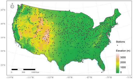
Figure 1.
The study area and the spatial distribution of ground stations, accessed from NOAA NCDC.
2.2. Ground Station Data
Monthly-averaged daily minimum and maximum temperature (Tmin and Tmax) data at 758 ground monitoring sites in 2015 were used for this study. The ground sites data was collected from the monthly dataset of the Global Historical Climatology Network (GHCN) data product provided by NOAA National Climatic Data Center. This monthly dataset was computed from the GHCN-daily product [48], which contains daily aggregated values for over 80,000 ground monitoring sites worldwide. The daily product integrates surface observations from multiple sources and was processed in a consistent manner with good quality control [49]. In this study, ground data was obtained by extracting ground stations in the conterminous United States in 2015 from the monthly dataset. The records with null values in the extracted data were discarded. Thus, a total of data records at 758 sites for 12 months in 2015 was used as our final modeling data. The 758 ground sites used in our study is displayed in Figure 1. As can be seen from the figure, the spatial locations of the ground sites were irregularly spaced across the entire study region. The western region had a lower coverage density compared to the eastern region. The statistics of the air temperatures were summarized in Table 1.

Table 1.
Summaries of air temperature (units: K).
2.3. Urban Areas Data
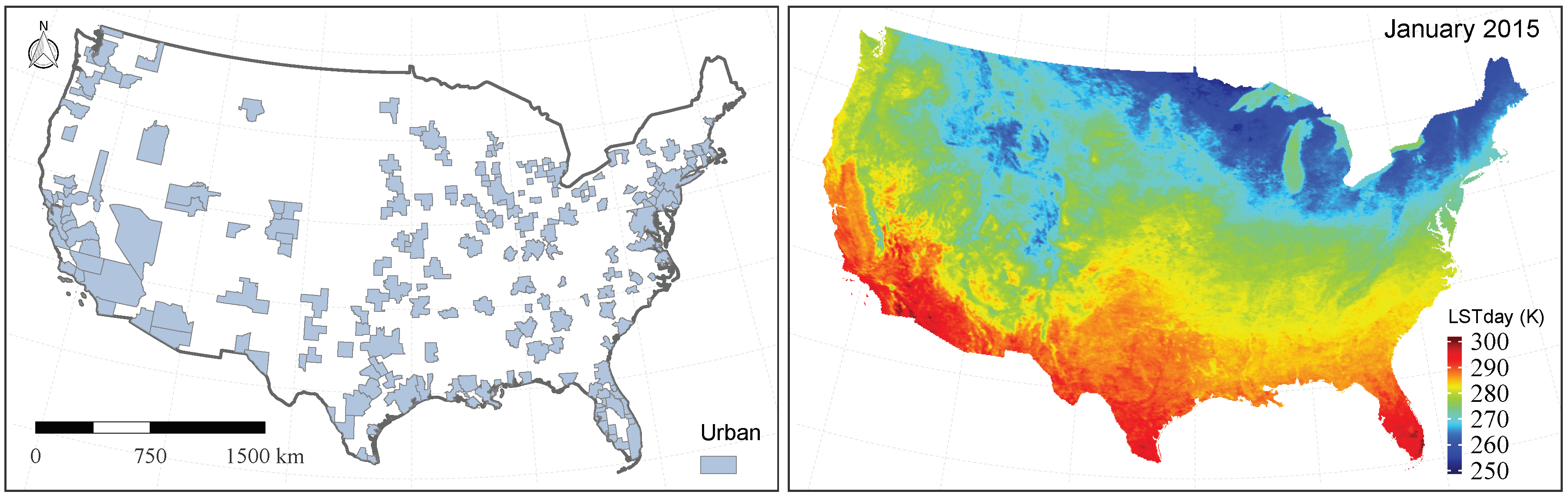
Urban areas are characterized by high population density and complex built environments. The complex surfaces composed of artificial materials and human activities have caused many urban environmental issue, especially the urban heat island effects [50]. As the air temperature is the key factor in evaluating and analyzing the urban heat environment, it is important to justify the predictive performance of the proposed method in the urban areas. In this study, functional urban areas were used to extract the modeling samples for ground sites in the urban areas. The functional urban areas (FUA) data was accessed from the OECD website (http://www.oecd.org/). The FUA dataset was jointly created by the OECD and the European Commission using population density and commuting travel flows data sources. A FUA unit consists of an urbanized city region and of a surrounding commuting zone. Figure 2 (left) shows the urban areas in the conterminous United States, which includes 211 area units. By overlaying the urban areas with the ground sites, a subset of 229 sites was obtained.

Figure 2.
(left) Urban areas in the conterminous United States, accessed from OECD. (right) The monthly daytime land surface temperature (LSTday) in January 2015, accessed from LAADS data archive.
2.4. Land Surface Temperature
The MODIS LST monthly composite product with a degree spatial resolution was used as the predictor variables for Ta estimation in our models. The MODIS LST was retrieved from the thermal observations of the MODIS sensor onboard both the Terra and the Aqua satellite by using a generalized split-window algorithm [51]. The overpass times are about 10:30 and 22:30 for Terra, 13:30 and 1:30 for Aqua at local time. The monthly data (MOD11C3) is a composite product based on averaging the daily MODIS LST product [52] and was accessed from the LAADS DAAS website. It should be noted that the daily MODIS LST data has missing values of different degrees mainly due to cloud contamination. The LST values in some regions of the monthly data may not have been good representatives for the monthly scale if the regions only had a few valid values in the month. The monthly LST data provides surface temperature values for both the daytime and nighttime cases. Figure 2 (right) shows the daytime LST in January 2015, which is colored in a linear scale. All collected data was preprocessed to generate a final formatted model data. The LST data together with locations of ground stations was projected from the WGS-84 geographic coordinate system to the planar cartesian coordinate system using the Lambert conformal conic projection. The projected monthly LST datasets were resampled at a 5 km spatial resolution. Then, the corresponding LST values at the ground sites were obtained by extracting the pixels of LST images where the sites fall in. Finally, a formatted data frame with 758 rows and seven variables including station identifier codes (ID), maximum air temperatures (Tmax), minimum air temperature (Tmin), daytime land surface temperature (LSTday) and nighttime land surface temperature (LSTnight), was created for each month in 2015.
3. Methods
3.1. Classical Kriging
Kriging is a geostatistical prediction technique widely used to interpolate grid values from observations measured at a set of sites. Kriging methods use random field (RF) to describe the underlying structure of spatially continuously variables. Basically, the RF is decomposed as follows:
where is a mean structure to model a large scale spatial trend of the RF; is a stationary random process with zero-mean and a known correlation function , which provides a way to characterize spatial dependence between pairs of locations . A variety of correlation functions are available. One typical example of stationary correlation function is an exponential one defined as with the parameter representing spatial variance and controlling spatial decay effects. is a euclidean distance between location and .
The representation of a spatial field in Equation (1) can be used to explain complex spatial patterns of variation in a spatial field. The mean structure from will filter out a large scale heterogeneous structure, while the stationary random process is used to capture a fine scale dependence structure. However, in classical Kriging techniques, the parametric type and parameters of the correlation function should be first estimated and computed from data. This estimated parameters are then plugged into the Kriging equation system (see [42,53] for details) to get predicted values at unobserved locations.
3.2. Bayesian Kriging Regression
The Bayesian Kriging regression (BKR) is a statistical Kriging model with a Gaussian assumption in the Bayesian framework. Since the Bayesian framework considers model parameters as random variables, BKR has the ability to quantify uncertainties associated with the model parameters. Specifically, the residual in Equation (1) is further decomposed as , where is a Gaussian process , is a Gaussian white noise . The mean structure can be explained by a set of covariates: , where is a vector of covariates values at location s, is the coefficients for the covariates. Denote the model parameters as . The meanings of parameters are described in Section 3.1. The parameter is a microscale random component, which usually represents measurement errors.
The BKR method to model and estimate Ta is specified for both the daytime and nighttime cases. In the case of the daytime models, let Tmax be a continuous random field where is the USA region and denotes the monthly averaged Tmax value measured at a spatial location s for a specific month. A total number of monthly Tmax values from the 758 ground stations, denoted as , a response matrix, can be viewed as a partial realization from the RF. is a design matrix for the intercept and the covariate LSTday. Then, the BKR model can be constructed as follows:
where is a vector for spatial random effects, which follows a multivariate Gaussian distribution with a covariance matrix computed from the correlation function ; is a random error vector with a covariance matrix , i.e., a diagonal matrix. The BKR method considers all the model parameters as random variables and assigns prior distributions to the paramters. Let be a prior distribution and be the posterior distribution of model paramters. Using the Bayes formula, the posterior distribution of can be computed by Equation (5), which will be used to quantify uncertainties in model paramters. The predictive distribution of Tmax at an unobserved location can be derived as Equation (6), which gives a way to describe uncentainties in estimated values.
where denotes the predicted Tmax at a location and is the covariate LSTday value at the location .
To compute results from the BKR model described above, a Gibbs Sampler algorithm was adopted, which is a widely-used type of Markov chain Monte Carlo (MCMC) methods. To be specific, an algorithm of four chains each with 5000 samples was specified. Due to no information about the model parameters, all the parameters were assigned non-informative or flat priors. Customarily, the coefficient vector follows a multivariate distribution with large variance and the spatial decay parameter follows a uniform distribution. Based on our research data, the prior was specified as . Samples of posterior and predictive distributions were computed from Equations (5) and (6) respectively. For more technical details about the Gibbs Sampler algorithm, refer to [47]. The R computing language and the spBayes package [54] were adopted to perform the BKR method.
3.3. Model Evaluation
To evaluate the model performance of the BKR method, linear regression method (LR) was compared with the BKR in the daytime and nighttime cases. Ten-fold cross-validation was used as the evaluation method and root mean square error (RMSE) was adopted as a quantitative evaluation indicator. RMSE is defined as follows:
where the is the number of samples, is an observed value, is the predicted value.
In this study, cross-validation was carried out under the whole region scenario where all data samples with 758 stations were used, and the urban areas scenario where a subset of 229 stations in the urban region were selected. For the whole region scenario, the general procedure can be described as follows: (1) a sample of 758 stations was randomly split into 10 subsamples with equal size; (2) one subsample was used as a validation set and the remaining 9 subsamples were used for modeling; (3) the fitted model was then applied to the validation set to compute a RMSE value; (4) the above process was repeated nine times until each subsample was used exactly once as the validation set. The procedure was carried out in each month of 2015 using both the LR method and BKR method.
4. Results and Discussion
4.1. Exploratory Data Analysis
A preliminary exploratory analysis was performed to explore the correlation between monthly Ta measured at stations and satellite-derived LST of all 758 sites in the study area. Previous studies have showed that daily Ta has a good agreement with daily LST. For example, Vogt et al. reported a high mean (coefficient of determination) of between daily Tmax and mean LST [7]. The study of Noi et al. showed a of 0.92 between daily Tmin and daily LSTnight from MODIS onboard Terra [17]. It was widely found that correlation between LSTnight and Tmin was relatively higher than correlation between LSTday and Tmax [19,21,34]. The purpose of this exploratory analysis is to confirm this agreement at the monthly level.
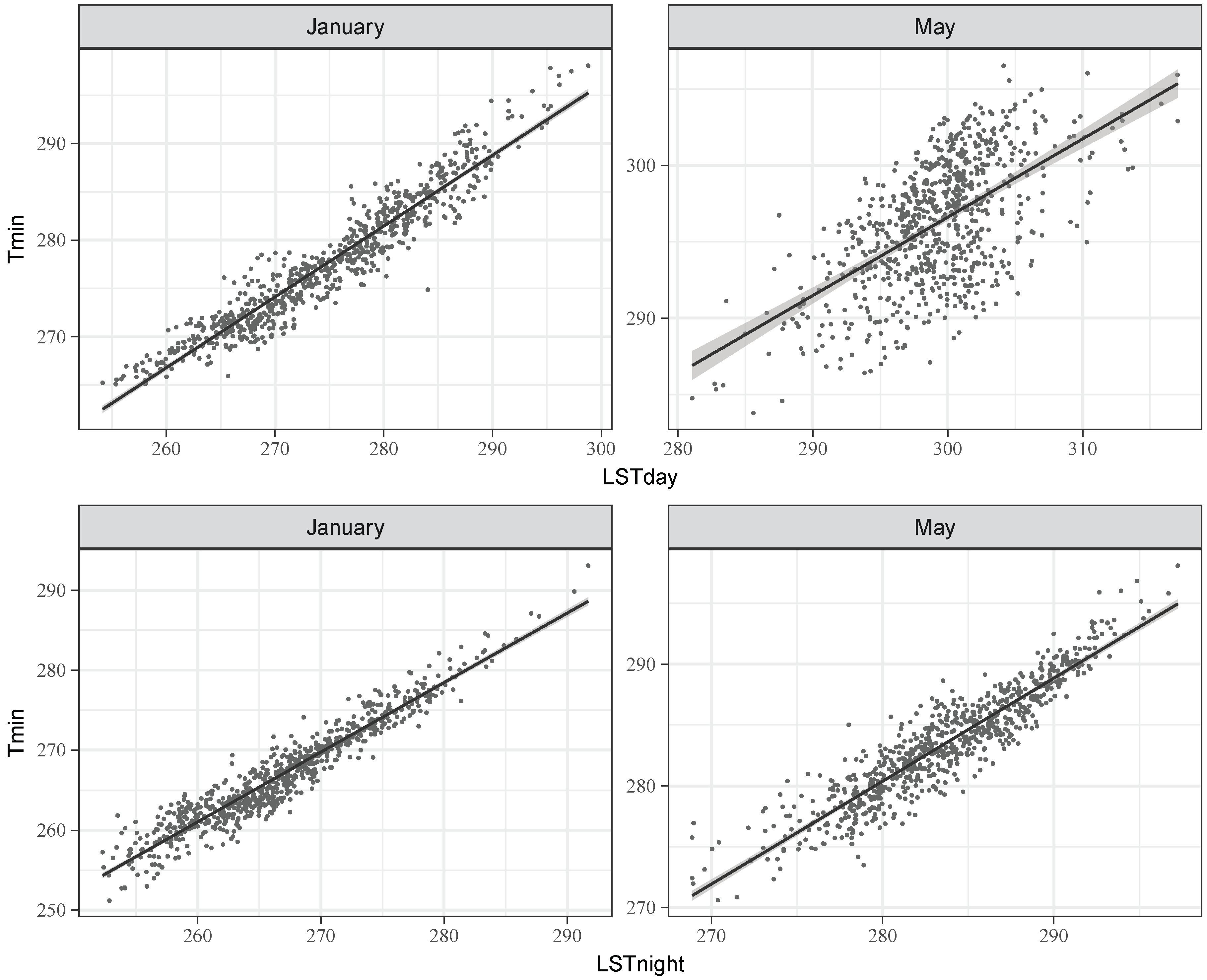
Figure 3 shows scatter plots of Tmax against LSTday (the daytime case) and Tmin against LSTnight (the nighttime case) for two selected months, January and May. The regression lines and its confidence interval represented by the gray strip around the lines are displayed for each plots. From the plots, it can be seen that the correlation in the nighttime case is stronger than the daytime case. The computed sample correlation coefficients () for all 12 months are summarized in Table 2, which indicates that on average, LST is highly correlated to observed Ta. In the nighttime case, the values of for 12 months are all above with an average of 0.94. In the daytime case, however, the relationship between Tmax and LSTday is more variable for different months (see the Daytime row in Table 2). Months from April to September have weak correlations with a minimum value in May in the daytime case. Although there is a significant variation in the correlations in the daytime case, Tmax has good agreements with LSTday in the spring (months 1–3) and the winter season (months 10–12) with an average of . Therefore, the night LST data can provide a better description of Ta than the daytime LST at the monthly temporal scale. Similar results have also been found at the monthly scale [15,40]. It is reasonable that monthly Ta can be estimated by a model using satellite-derived LST data as the only input.
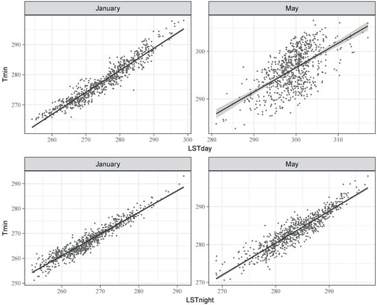
Figure 3.
Scatter plots between surface air temperature (Ta) and land surface temperature (LST) for two selected months: (top row) plots of maximum temperature (Tmax) against LSTday. (bottom row) Plots of minimum temperature (Tmin) against LSTnight.
Table 2.
Values of in daytime and nighttime cases for each month of 2015.
Linear regression (LR) is the most popular method in estimating Ta due to its simplicity and high explanatory power. The study by Vogt et al. is the first to apply the LR method to estimate daily Tmax using only LST data as the covariate [7]. Many studies have used the LR approach to relate Ta with LST and other covariates such as NDVI, solar zenith angel, elevation and latitudes. To assess and analyze model performance of LR in this study dataset, LR models using the LST data as the covariate were fitted in both the daytime and the nighttime cases.
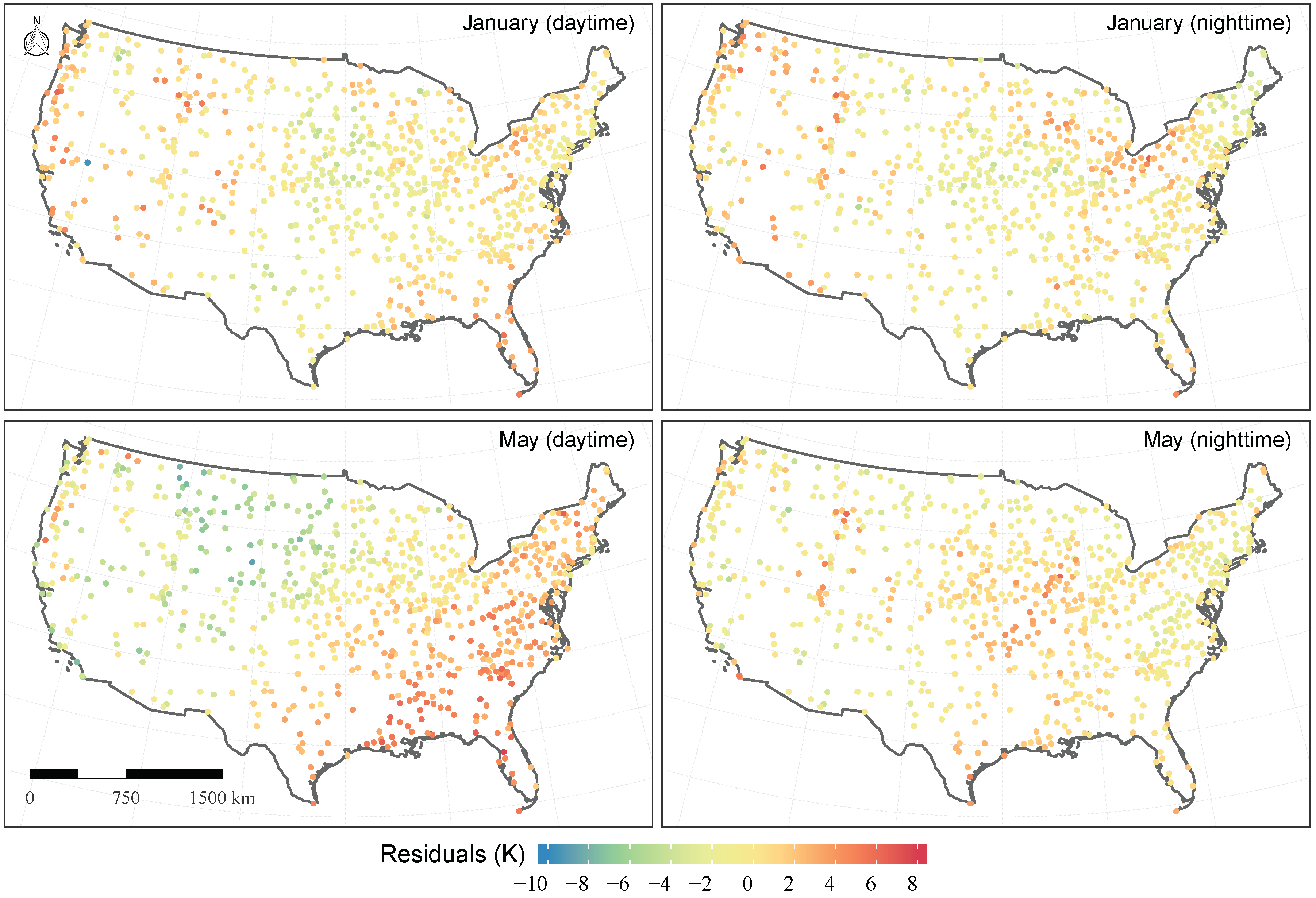
The daytime models used LSTday to estimate Tmax in each month. The nighttime models used LSTnight to estimate Tmin in each month. The residuals from the models in January and May were mapped in Figure 4. It can be seen from Figure 4 that the model residuals have clear spatial patterns and different spatial dependence structures. For example, the daytime model and the nighttime model in January tend to overestimate Tmax in the eastern and western areas and underestimate Tmax in central plains. For May, the daytime model overestimated Tmax in southeastern part and the nighttime model generally led to an overestimation over the whole study region. However, the residuals represent a fine scale structure of Ta field and the LR method has failed to capture this fine structure. Therefore, a more reliable estimation will be obtained when considering and explicitly modeling the fine scale structure.
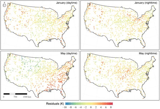
Figure 4.
Spatial distributions of residuals in the linear regression (LR) models (top left: the LR model in the daytime case in January).
4.2. Cross Validation
The LR method used LST to model the large spatial trend of Ta, but it cannot capture the fine spatial structure in the residuals from the LR models. The BKR method not only can explicitly model the fine spatial structure by a Gaussian random field, but also has the ability to quantify uncertainties. Thus, the BKR method will provide a better description of the complex spatial variability of Ta. As a result, better prediction performance will be obtained from the BKR models. To validate this assertion, the BRK method was compared to the LR method using 10-fold cross-validation approach for both the whole region and the urban areas of the conterminous United States. In the whole region scenario, a total of 758 site samples for each month were used in the cross-validation procedure. For the urban areas, a subset of 229 sites were extracted firstly from the complete 758 sites using the urban areas data and then used in the cross-validation.
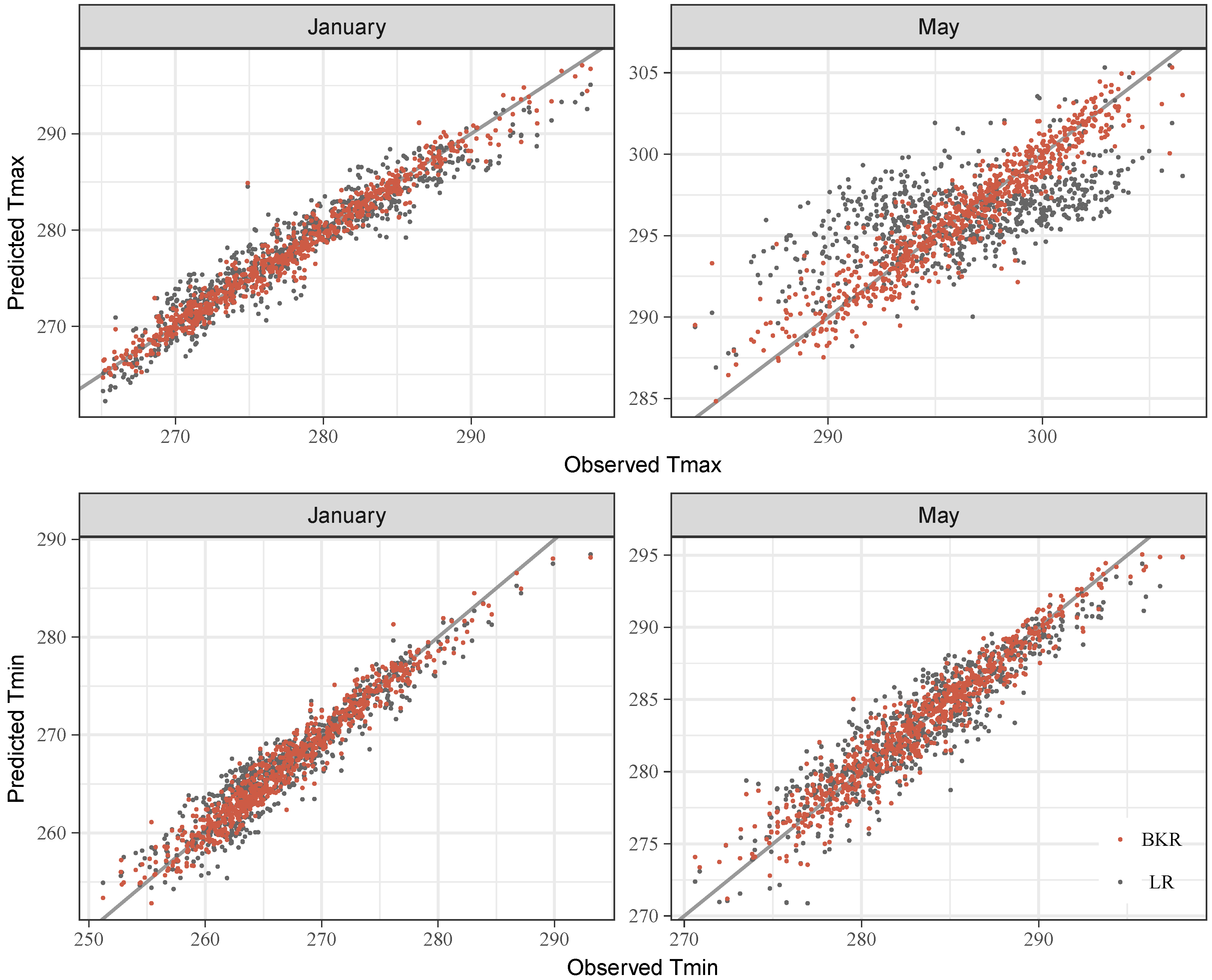
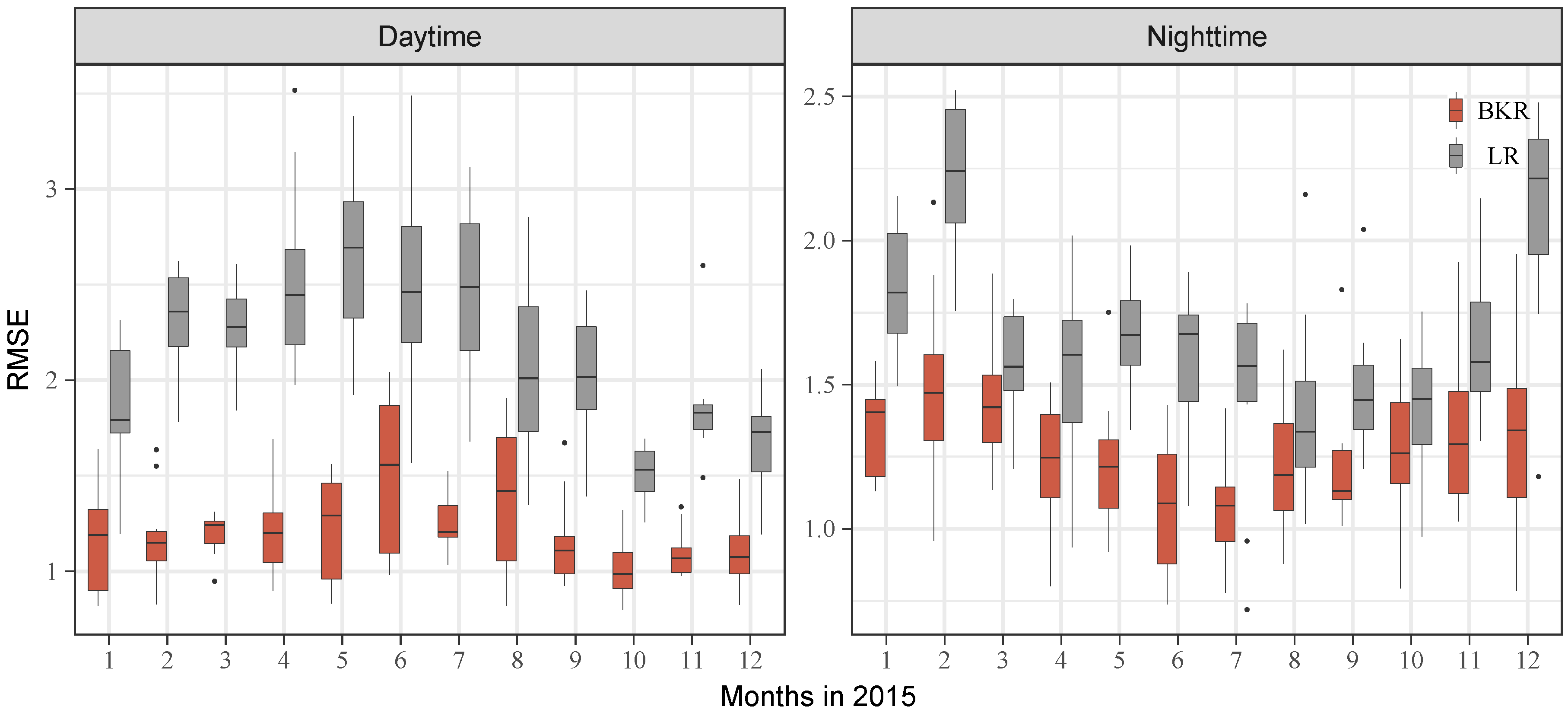
Figure 5 represents the scatter plots of observed Ta against predicted Ta from the LR models (gray color) and the BKR models (red color) under the whole region scenario. Improved prediction performance of the BKR method can be confirmed by a visual examination of the figure. To quantify the improvement of the BKR method, RMSE values of the two methods were computed for each month in 2015. For each month, 10 RMSE values from the 10-fold cross-validation are graphed in a boxplot for the two methods. A boxplot characterizes the distribution of 10 RMSE values for each month by using the quartiles. The central rectangle depicts the range (the interquartile range (IQR)) between the first quartile and the third quartile. The segment inside the rectangle denotes the median of the values. Two vertical lines (whiskers) above and below the rectangle each represent a range of IQR. Outliers are displayed as dot points, which are either IQR or more above the third quartile or below the first quartile.
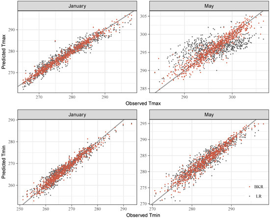
Figure 5.
The whole region scenario: observed Ta against predicted Ta from LR and Bayesian Kriging regression (BKR): (top row) models in the daytime case (Tmax). (bottom row) Models in the nighttime case (Tmin).
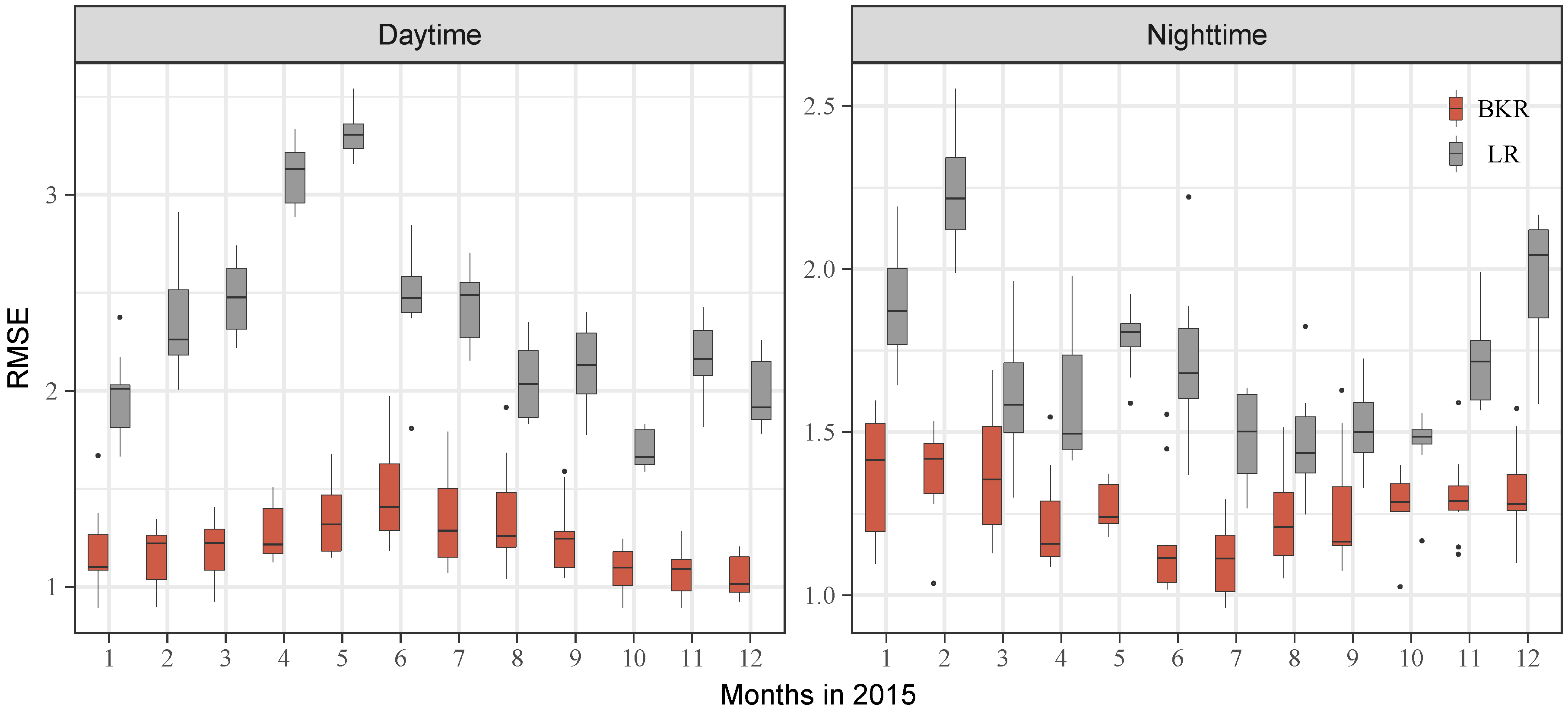
Figure 6 represents boxplots of RMSE for 12 months under the whole region scenario. From Figure 6, we can see that the BKR method had a lower RMSE for all 12 months in both the daytime (Figure 6, right) and nighttime cases (Figure 6, left). In the daytime case, the average RMSE values of the two methods is K for the LR method and K for the BKR method. In the nighttime case, the LR method had an average RMSE of K, and the BKR method had an average of RMSE K. From the results, the BKR method achieved averaged RMSE values of K for Tmax and K for Tmin. The model performance of the BKR method in this study was relatively better than similar studies on the estimation of monthly Ta. Lu et al. used a hierarchical space–time model to estimate monthly Ta over the Qinghai Province in China and achieved RMSE values of K for Tmax and K for Tmin [40]. Chen et al. achieved RMSE values of K for Tmax and K Tmin using geographically weighted regression (GWR) [15]. Wang et al. compared different methods in estimating monthly Ta and found that GWR has a similar prediction performance to that of Kriging regression [35]. A RMSE of K for estimating monthly mean Ta was obtained using machine learning algorithms with a set of inputs [27]. In addition to the improved prediction performance in an averagely sense, the RMSE values of the BKR method for different months are more stable with a lower value compared to the LR method, which is illustrated by a steady fluctuation of the red boxplots in Figure 6. In particular, RMSE values of the LR method in the daytime case for the months of 4, 5, 6, 7 (the summer season) in 2015 are more deviated from the average level. For the LR method in the nighttime case, the months of 12, 1, 2 are more deviated.
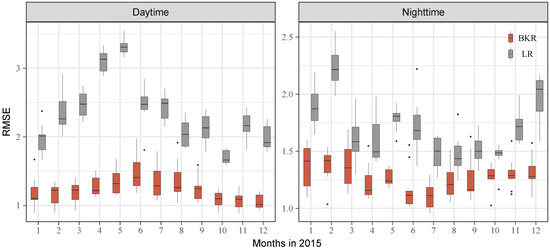
Figure 6.
The whole region scenario: boxplot of root mean squared error (RMSE) of the LR and BKR for 12 months in 2015: (left) models in the daytime case (Tmax). (right) Models in the nighttime case (Tmin).
As for the urban areas scenario, the summarized statistical description of the cross-validation RMSE values is also represented by the boxplot in Figure 7. It can be seen from the plot that the BKE method achieved a similar predictive performance compared to the results from the cross-validation for the whole region. The averaged RMSE values of the BKR method are K for Tmax and K for Tmin. The BKR method is also superior to the linear regression method for different months and the two cases (the daytime and nighttime cases). The results of the urban areas scenario indicate that the BKR method is also valid for estimating monthly Ta using the LST data in the urban areas.

Figure 7.
The urban areas scenario: boxplot of RMSEs of the LR and BKR for 12 months in 2015: (left) models in the daytime case (Tmax). (right) Models in the nighttime case (Tmin).
4.3. Model Fitting
All the data samples of 758 sites were used to fit the BKR models for each month of 2015 in the daytime and nighttime cases. A total of fitted models were obtained. As the BKR method had the ability to quantify the uncertainties in model parameters by posterior distributions, we obtained 10,000 posterior sample values for each model parameter in each fitted model. The fitted model parameters for Jan and May were summarized in Table 3 using three percentiles ().
Table 3.
Posterior parameter percentiles of fitted models in January and May of 2015.
In Table 3, and represent coefficients of the model intercept and LST respectively; and denote the spatial variance and the error variance; is the spatial decay parameter. To give an intuitive view of the posteriors of the parameters, histograms of the and samples in the fitted daytime model in January are displayed in Figure 8. The summarized statistical numbers in Table 3 can be used to evaluate uncertainties in the fitted models. In comparison to other models, the coefficient of LST of the nighttime model in January had the highest credible interval (CI) from to , but the of the daytime model in May had the lowest CI from to . The spatial decay parameters of the four models generally had a similar value around , but this parameter has a narrower CI for models in January than for models in May (CI ). A similar pattern has been found for the spatial variance , where CIs of the parameter for models in January were lower than models in May. In terms of the error variance , it can be found that it had a stable CI around among the four models.
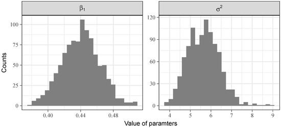
Figure 8.
The posterior distributions of the coefficient of LST () and the spatial variance () of the daytime model in January.
The median values of the model parameters of all fitted models are summarized in Table 4. From Table 4, we can see that the coefficient of LST () is generally higher in the nighttime case than the daytime case. However, the spatial variance parameter () was higher in the daytime case than in the nighttime case. This was probably caused by the high spatial variability of Tmax in the daytime and more spatial structure information in Tmax was captured by the model, which is indicated by the high spatial variance parameter. The spatial decay parameter () was stable around for all models, which means that Ta had a similar spatial dependence in different months when the large spatial trend was explained by the LST.
Table 4.
Parameter medians of the daytime and nighttime models for each month in 2015.
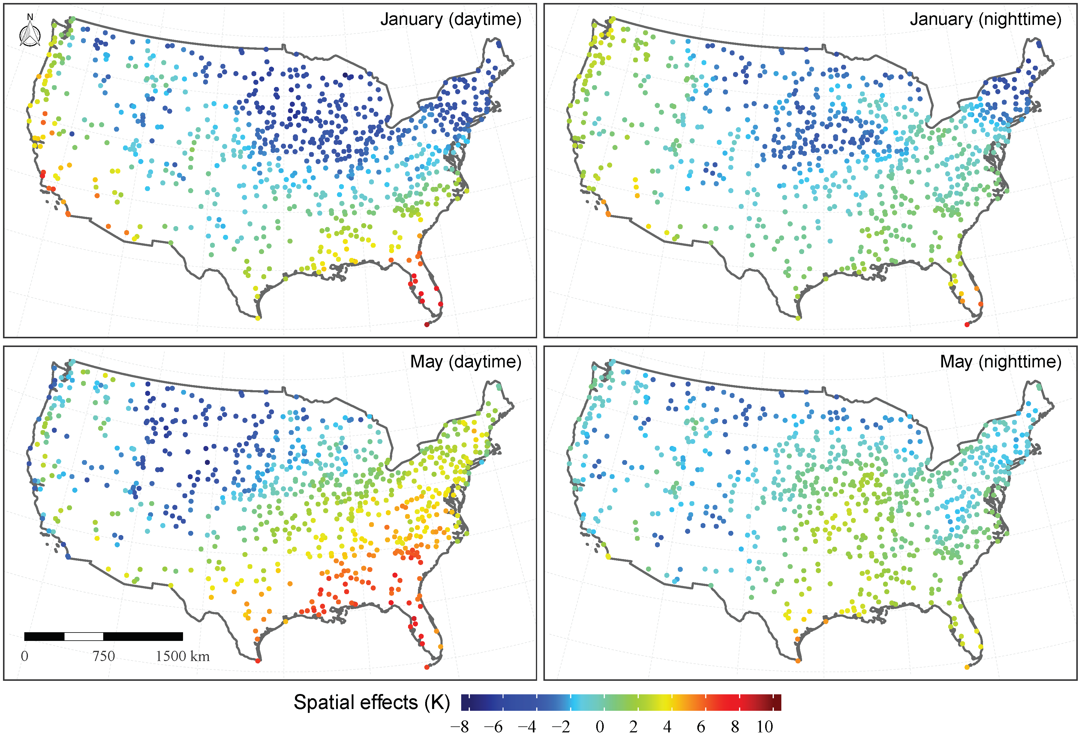
One advantage of the BKR was its ability to fit the spatial random effect of Ta. This effects is the fitted value of the Gaussian process at the sample sites of the BKR model (see Section 3.2 for details). Figure 9 shows the distributions of the fitted spatial effects for models in January and May. It can be clearly seen from Figure 9 that different spatial patterns are revealed in the maps. These spatial patterns represent the unexplained fine scale spatial structure of Ta. Comparing these patterns with LR models residuals in Figure 4 (Section 4.1), we can find better matches between them, which means that the Gaussian process in the BKR model has captured the structure in the residuals that the LR models failed to capture. The fine scale spatial structure together with large scale spatial trend explained by the LST variable provide a better description of the complex structure in the Ta field.

Figure 9.
Spatial distributions of fitted spatial random effects in the fitted BKR models (top left: the daytime model in January).
4.4. Air Temperature Estimation
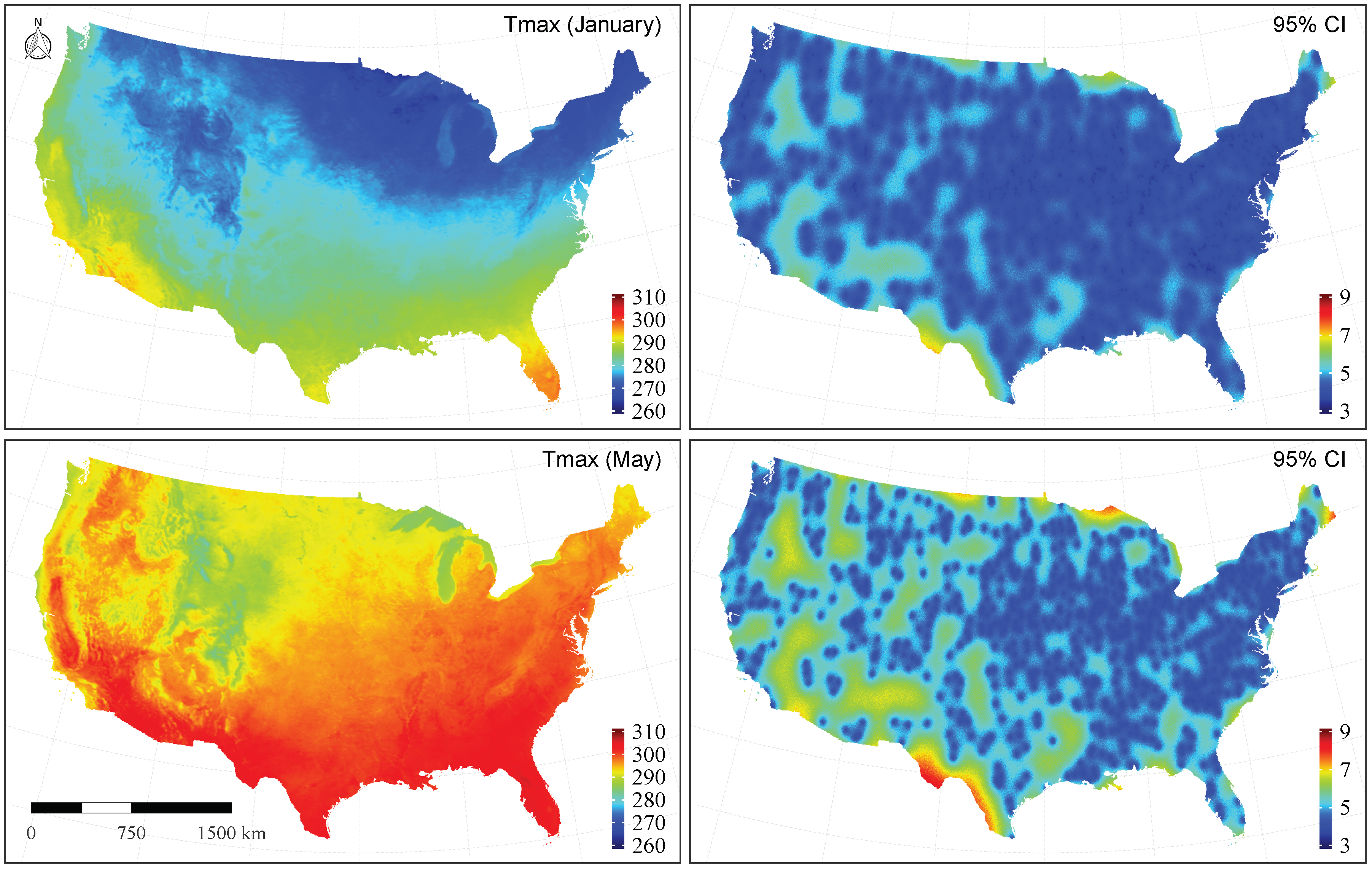
The fitted models were used to estimate Tmax and Tmin for each month of 2015 at locations without ground stations. As the covariate variables LSTday and LSTnight were a gridded image with 5 km resolution, predicted Tmax and Tmin represent averaged values in each grid or pixel. By sampling from the predictive distribution in the fitted models, a total of 10,000 predicted samples was obtained for each pixel. The predicted samples for each pixel give a full description of the uncertainty in the predicted value. The Figure 10 shows the estimated Tmax in January and May as well as its credible intervals (CI). The estimated value of Tmax of one pixel is the median value of the samples for the pixel. The CI of one pixel is computed as the difference between the and percentiles of the samples. The map of CI in January shows that the most areas of USA have relatively low CI interval values between 3–4 K, indicating a more reliable estimation. The CI map in May has relatively high CI interval values in some parts of the western region, which have complex topographic features. The two CI maps indicate that the estimated Tmax in January is more reliable than the estimated Tmax in May.
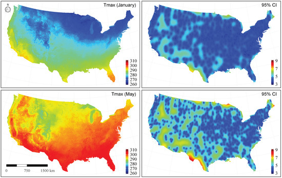
Figure 10.
Estimation of Tmax in January and May: (top row) maps of estimated Tmax and its credible intervals (CI) in January. (bottom row) Maps of estimated Tmax and its CI in May.
5. Conclusions
In this paper, a Bayesian Kriging regression (BKR) method was proposed to model and estimate monthly air temperature (Ta) using land surface temperature (LST) as the only covariate. The BKR method is a spatial statistical model which decomposes the spatial variability of Ta into a large scale trend and a fine scale spatial structure. By embedding the Kriging regression into the Bayesian Framework, the BKR has the capacity to quantify uncertainties in both model parameters and predicted Ta values. Specifically, this study has developed models to estimate monthly maximum air temperature (Tmax) using daytime LST, and to estimate monthly minimum air temperature (Tmin) using nighttime LST in 2015 over the conterminous United States. The uncertainties in the parameters of developed models and estimated Ta were both analyzed.
An exploratory analysis shows a generally close relationship between LST and Ta. The correlation between Tmin and nighttime LST is relatively higher than that between Tmax and daytime LST. The results indicate that it is reasonable to estimate monthly Ta using only LST data. A 10-fold cross-validation approach was adopted to compare the predictive performance of the BKR method and the LR method for the whole region and the urban areas of the conterminous Unite States. The results for the whole region show that the BKR method achieves a competitively better performance with averaged RMSE values K for Tmax and K for Tmin. Compared with few previous studies on estimating monthly Tmax and Tmin, the BKR method can obtain the best predictive performance. But the RMSE values reported in the previous studies should considered critically due to different study areas and datasets. In addition, the cross-validation results for the urban areas demonstrates a similar performance with the whole region. In conclusion, all the results prove that the BKR method using only LST data can obtain a relatively better predictive performance. Additionally, posterior samples of the model parameters and predictive samples of the estimated Ta were obtained. These samples can be used to quantify uncertainties in model parameters and estimated Ta values.
However, there is a major limitation regarding the BKR method. The samples of the model parameters and estimated Ta were generated by a MCMC algorithm such as the Gibbers Sampler. As this sampling was done for each pixel to be estimated, a large computation time and storage space will be used when estimating Ta over a large region with finer spatial resolution. Because of the MCMC sampling algorithm is highly scalable in computation, this limitation can be addressed by using parallel computing over multiple cores.
Author Contributions
Q.D. and Z.Z. conceived the idea; Z.Z. designed the experiments, processed the data and implemented the model; Q.D. and Z.Z. discussed and analyzed the results; Z.Z. wrote the paper; Q.D. made some suggestions on the paper.
Funding
This research was supported by the National Key Research and Development Program of China (2016YFC0803106) and the National Natural Science Foundation of China (Project No. 41871355).
Acknowledgments
We greatly thank NOAA NCEI for providing GHCN-Monthly Version 3 datasets (https://www.ncdc.noaa.gov/ghcnm/v3.php), LAADS DAAS for providing MODIS LST datasets (https://lpdaac.usgs.gov/node/826) and OECD for providing vector data of functional urban areas in the conterminous United States (http://www.oecd.org/cfe/regional-policy/functionalurbanareasbycountry.htm). Additionally, we deeply appreciate the R, an open source statistical computing environment (https://www.r-project.org).
Conflicts of Interest
The authors declare no conflict of interest.
References
- Braga, A.L.F.; Zanobetti, A.; Schwartz, J. The effect of weather on respiratory and cardiovascular deaths in 12 U.S. cities. Environ. Health Perspect. 2002, 110, 859–863. [Google Scholar] [CrossRef] [PubMed]
- Basu, R. Relation between Elevated Ambient Temperature and Mortality: A Review of the Epidemiologic Evidence. Epidemiol. Rev. 2002, 24, 190–202. [Google Scholar] [CrossRef]
- Scovronick, N.; Sera, F.; Acquaotta, F.; Garzena, D.; Fratianni, S.; Wright, C.Y.; Gasparrini, A. The association between ambient temperature and mortality in South Africa: A time-series analysis. Environ. Res. 2018, 161, 229–235. [Google Scholar] [CrossRef] [PubMed]
- Ragettli, M.S.; Vicedo-Cabrera, A.M.; Schindler, C.; Röösli, M. Exploring the association between heat and mortality in Switzerland between 1995 and 2013. Environ. Res. 2017, 158, 703–709. [Google Scholar] [CrossRef] [PubMed]
- Lin, Y.K.; Maharani, A.T.; Chang, F.T.; Wang, Y.C. Mortality and morbidity associated with ambient temperatures in Taiwan. Sci. Total Environ. 2019, 651, 210–217. [Google Scholar] [CrossRef]
- Vancutsem, C.; Ceccato, P.; Dinku, T.; Connor, S.J. Evaluation of MODIS land surface temperature data to estimate air temperature in different ecosystems over Africa. Remote Sens. Environ. 2010, 114, 449–465. [Google Scholar] [CrossRef]
- Vogt, J.V.; Viau, A.A.; Paquet, F. Mapping regional air temperature fields using satellite-derived surface skin temperatures. Int. J. Climatol. 1997, 17, 1559–1579. [Google Scholar] [CrossRef]
- Prihodko, L.; Goward, S.N. Estimation of air temperature from remotely sensed surface observations. Remote Sens. Environ. 1997, 60, 335–346. [Google Scholar] [CrossRef]
- Prince, S.; Goetz, S.; Dubayah, R.; Czajkowski, K.; Thawley, M. Inference of surface and air temperature, atmospheric precipitable water and vapor pressure deficit using Advanced Very High-Resolution Radiometer satellite observations: Comparison with field observations. J. Hydrol. 1998, 212–213, 230–249. [Google Scholar] [CrossRef]
- Benali, A.; Carvalho, A.; Nunes, J.; Carvalhais, N.; Santos, A. Estimating air surface temperature in Portugal using MODIS LST data. Remote Sens. Environ. 2012, 124, 108–121. [Google Scholar] [CrossRef]
- Willmott, C.J.; Robeson, S.M. Climatologically aided interpolation (CAI) of terrestrial air temperature. Int. J. Climatol. 1995, 15, 221–229. [Google Scholar] [CrossRef]
- Courault, D.; Monestiez, P. Spatial interpolation of air temperature according to atmospheric circulation patterns in southeast France. Int. J. Climatol. 1999, 19, 365–378. [Google Scholar] [CrossRef]
- Cresswell, M.P.; Morse, A.P.; Thomson, M.C.; Connor, S.J. Estimating surface air temperatures, from Meteosat land surface temperatures, using an empirical solar zenith angle model. Int. J. Remote Sens. 1999, 20, 1125–1132. [Google Scholar] [CrossRef]
- Mostovoy, G.V.; King, R.L.; Reddy, K.R.; Kakani, V.G.; Filippova, M.G. Statistical Estimation of Daily Maximum and Minimum Air Temperatures from MODIS LST Data over the State of Mississippi. GISci. Remote Sens. 2006, 43, 78–110. [Google Scholar] [CrossRef]
- Chen, F.; Liu, Y.; Liu, Q.; Qin, F. A statistical method based on remote sensing for the estimation of air temperature in China. Int. J. Climatol. 2015, 35, 2131–2143. [Google Scholar] [CrossRef]
- Good, E. Daily minimum and maximum surface air temperatures from geostationary satellite data: Satellite min and max air temperatures. J. Geophys. Res. Atmos. 2015, 120, 2306–2324. [Google Scholar] [CrossRef]
- Noi, P.; Kappas, M.; Degener, J. Estimating Daily Maximum and Minimum Land Air Surface Temperature Using MODIS Land Surface Temperature Data and Ground Truth Data in Northern Vietnam. Remote Sens. 2016, 8, 1002. [Google Scholar] [CrossRef]
- Zakšek, K.; Schroedter-Homscheidt, M. Parameterization of air temperature in high temporal and spatial resolution from a combination of the SEVIRI and MODIS instruments. ISPRS J. Photogramm. Remote Sens. 2009, 64, 414–421. [Google Scholar] [CrossRef]
- Yoo, C.; Im, J.; Park, S.; Quackenbush, L.J. Estimation of daily maximum and minimum air temperatures in urban landscapes using MODIS time series satellite data. ISPRS J. Photogramm. Remote Sens. 2018, 137, 149–162. [Google Scholar] [CrossRef]
- Stisen, S.; Sandholt, I.; Nørgaard, A.; Fensholt, R.; Eklundh, L. Estimation of diurnal air temperature using MSG SEVIRI data in West Africa. Remote Sens. Environ. 2007, 110, 262–274. [Google Scholar] [CrossRef]
- Zhu, W.; Lű, A.; Jia, S. Estimation of daily maximum and minimum air temperature using MODIS land surface temperature products. Remote Sens. Environ. 2013, 130, 62–73. [Google Scholar] [CrossRef]
- Kitsara, G.; Papaioannou, G.; Retalis, A.; Paronis, D.; Kerkides, P. Estimation of air temperature and reference evapotranspiration using MODIS land surface temperature over Greece. Int. J. Remote Sens. 2018, 39, 924–948. [Google Scholar] [CrossRef]
- Sun, Y.J.; Wang, J.F.; Zhang, R.H.; Gillies, R.R.; Xue, Y.; Bo, Y.C. Air temperature retrieval from remote sensing data based on thermodynamics. Theor. Appl. Climatol. 2005, 80, 37–48. [Google Scholar] [CrossRef]
- Moser, G.; De Martino, M.; Serpico, S.B. Estimation of Air Surface Temperature From Remote Sensing Images and Pixelwise Modeling of the Estimation Uncertainty Through Support Vector Machines. IEEE J. Sel. Top. Appl. Earth Obs. Remote Sens. 2015, 8, 332–349. [Google Scholar] [CrossRef]
- Meyer, H.; Katurji, M.; Appelhans, T.; Müller, M.; Nauss, T.; Roudier, P.; Zawar-Reza, P. Mapping Daily Air Temperature for Antarctica Based on MODIS LST. Remote Sens. 2016, 8, 732. [Google Scholar] [CrossRef]
- Zhang, H.; Zhang, F.; Ye, M.; Che, T.; Zhang, G. Estimating daily air temperatures over the Tibetan Plateau by dynamically integrating MODIS LST data. J. Geophys. Res. Atmos. 2016, 121, 11425–11441. [Google Scholar] [CrossRef]
- Xu, Y.; Knudby, A.; Shen, Y.; Liu, Y. Mapping Monthly Air Temperature in the Tibetan Plateau From MODIS Data Based on Machine Learning Methods. IEEE J. Sel. Top. Appl. Earth Obs. Remote Sens. 2018, 11, 345–354. [Google Scholar] [CrossRef]
- Mira, M.; Ninyerola, M.; Batalla, M.; Pesquer, L.; Pons, X. Improving Mean Minimum and Maximum Month-to-Month Air Temperature Surfaces Using Satellite-Derived Land Surface Temperature. Remote Sens. 2017, 9, 1313. [Google Scholar] [CrossRef]
- Zhu, W.; Lű, A.; Jia, S.; Yan, J.; Mahmood, R. Retrievals of all-weather daytime air temperature from MODIS products. Remote Sens. Environ. 2017, 189, 152–163. [Google Scholar] [CrossRef]
- Zhou, W.; Peng, B.; Shi, J.; Wang, T.; Dhital, Y.; Yao, R.; Yu, Y.; Lei, Z.; Zhao, R. Estimating High Resolution Daily Air Temperature Based on Remote Sensing Products and Climate Reanalysis Datasets over Glacierized Basins: A Case Study in the Langtang Valley, Nepal. Remote Sens. 2017, 9, 959. [Google Scholar] [CrossRef]
- Janatian, N.; Sadeghi, M.; Sanaeinejad, S.H.; Bakhshian, E.; Farid, A.; Hasheminia, S.M.; Ghazanfari, S. A statistical framework for estimating air temperature using MODIS land surface temperature data. Int. J. Climatol. 2017, 37, 1181–1194. [Google Scholar] [CrossRef]
- Kloog, I.; Nordio, F.; Lepeule, J.; Padoan, A.; Lee, M.; Auffray, A.; Schwartz, J. Modelling spatio-temporally resolved air temperature across the complex geo-climate area of France using satellite-derived land surface temperature data. Int. J. Climatol. 2017, 37, 296–304. [Google Scholar] [CrossRef]
- Pelta, R.; Chudnovsky, A.A. Spatiotemporal estimation of air temperature patterns at the street level using high resolution satellite imagery. Sci. Total Environ. 2017, 579, 675–684. [Google Scholar] [CrossRef] [PubMed]
- Rosenfeld, A.; Dorman, M.; Schwartz, J.; Novack, V.; Just, A.C.; Kloog, I. Estimating daily minimum, maximum, and mean near surface air temperature using hybrid satellite models across Israel. Environ. Res. 2017, 159, 297–312. [Google Scholar] [CrossRef] [PubMed]
- Wang, M.; He, G.; Zhang, Z.; Wang, G.; Zhang, Z.; Cao, X.; Wu, Z.; Liu, X. Comparison of Spatial Interpolation and Regression Analysis Models for an Estimation of Monthly Near Surface Air Temperature in China. Remote Sens. 2017, 9, 1278. [Google Scholar] [CrossRef]
- Li, X.; Zhou, Y.; Asrar, G.R.; Zhu, Z. Developing a 1 km resolution daily air temperature dataset for urban and surrounding areas in the conterminous United States. Remote Sens. Environ. 2018, 215, 74–84. [Google Scholar] [CrossRef]
- Florio, E.N.; Lele, S.R.; Chi Chang, Y.; Sterner, R.; Glass, G.E. Integrating AVHRR satellite data and NOAA ground observations to predict surface air temperature: A statistical approach. Int. J. Remote Sens. 2004, 25, 2979–2994. [Google Scholar] [CrossRef]
- Oyler, J.W.; Ballantyne, A.; Jencso, K.; Sweet, M.; Running, S.W. Creating a topoclimatic daily air temperature dataset for the conterminous United States using homogenized station data and remotely sensed land skin temperature. Int. J. Climatol. 2015, 35, 2258–2279. [Google Scholar] [CrossRef]
- Parmentier, B.; McGill, B.J.; Wilson, A.M.; Regetz, J.; Jetz, W.; Guralnick, R.; Tuanmu, M.N.; Schildhauer, M. Using multi-timescale methods and satellite-derived land surface temperature for the interpolation of daily maximum air temperature in Oregon. Int. J. Climatol. 2015, 35, 3862–3878. [Google Scholar] [CrossRef]
- Lu, N.; Liang, S.; Huang, G.; Qin, J.; Yao, L.; Wang, D.; Yang, K. Hierarchical Bayesian space-time estimation of monthly maximum and minimum surface air temperature. Remote Sens. Environ. 2018, 211, 48–58. [Google Scholar] [CrossRef]
- Diggle, P.J.; Tawn, J.A.; Moyeed, R.A. Model-based geostatistics. J. R. Stat. Soc. Ser. C Appl. Stat. 2002, 47, 299–350. [Google Scholar] [CrossRef]
- Hengl, T.; Heuvelink, G.B.; Rossiter, D.G. About regression-kriging: From equations to case studies. Comput. Geosci. 2007, 33, 1301–1315. [Google Scholar] [CrossRef]
- Al-Mudhafar, W.J. Bayesian kriging for reproducing reservoir heterogeneity in a tidal depositional environment of a sandstone formation. J. Appl. Geophys. 2019, 160, 84–102. [Google Scholar] [CrossRef]
- Wojciech, M. Kriging Method Optimization for the Process of DTM Creation Based on Huge Data Sets Obtained from MBESs. Geosciences 2018, 8, 433. [Google Scholar] [CrossRef]
- Handcock, M.S.; Stein, M.L. A Bayesian Analysis of Kriging. Technometrics 1993, 35, 403–410. [Google Scholar] [CrossRef]
- Le, N.D.; Zidek, J.V. Statistical Analysis of Environmental Space-Time Processes; Springer: New York, NY, USA, 2006; pp. 119–121. [Google Scholar]
- Banerjee, S.; Carlin, B.P.; Gelfand, A.E. Hierarchical Modeling and Analysis for Spatial Data; Chapman and Hall: Boca Raton, FL, USA, 2014; pp. 12–18. [Google Scholar]
- Menne, M.J.; Durre, I.; Korzeniewski, B.; McNeal, S.; Thomas, K.; Yin, X.; Anthony, S.; Ray, R.; Vose, R.S.; Gleason, B.E.; Houston, T.G. Global Historical Climatology Network-Daily (GHCN-Daily), version 3; NOAA National Climatic Data Center: Asheville, NC, USA, 2012. [Google Scholar]
- Menne, M.J.; Durre, I.; Vose, R.S.; Gleason, B.E.; Houston, T.G. An Overview of the Global Historical Climatology Network-Daily Database. J. Atmos. Ocean. Technol. 2012, 29, 897–910. [Google Scholar] [CrossRef]
- Sobrino, J.A.; Oltra-Carrió, R.; Sòria, G.; Jiménez-Muñoz, J.C.; Franch, B.; Hidalgo, V.; Mattar, C.; Julien, Y.; Cuenca, J.; Romaguera, M.; et al. Evaluation of the surface urban heat island effect in the city of Madrid by thermal remote sensing. Int. J. Remote Sens. 2013, 34, 3177–3192. [Google Scholar] [CrossRef]
- Wan, Z.; Dozier, J. A generalized split-window algorithm for retrieving land-surface temperature from space. IEEE Trans. Geosci. Remote Sens. 1996, 34, 892–905. [Google Scholar]
- Wan, Z.; Hook, S.; Hulley, G. MOD11C3 MODIS/Terra Land Surface Temperature/Emissivity Monthly L3 Global 0.05Deg CMG V006; NASA LP DAAC: Sioux Falls, SD, USA, 2015. [Google Scholar]
- Cressie, N.A.C. Statistics for sPatial Data; Wiley-Interscience: New York, NY, USA, 1993; pp. 105–112. [Google Scholar]
- Finley, A.O.; Banerjee, S.; Gelfand, A.E. spBayes for Large Univariate and Multivariate Point-Referenced Spatio-Temporal Data Models. J. Stat. Softw. 2015, 63. [Google Scholar] [CrossRef]


© 2019 by the authors. Licensee MDPI, Basel, Switzerland. This article is an open access article distributed under the terms and conditions of the Creative Commons Attribution (CC BY) license (http://creativecommons.org/licenses/by/4.0/).