Article

Soil Moisture Variability in India: Relationship of Land Surface–Atmosphere Fields Using Maximum Covariance Analysis

1
Department of Earth System Science, University of California, Irvine, CA 92697, USA
2
Jet Propulsion Laboratory, California Institute of Technology, Pasadena, CA 91109, USA
3
Department of Physics, Sri Venkateswara University, Tirupati 517502, India
4
National Atmospheric Research Laboratory, Gadanki 517112, India
*
Author to whom correspondence should be addressed.
Remote Sens. 2019, 11(3), 335; https://doi.org/10.3390/rs11030335
Submission received: 19 December 2018 / Revised: 1 February 2019 / Accepted: 2 February 2019 / Published: 8 February 2019
(This article belongs to the Special Issue Assimilation of Remote Sensing Data into Earth System Models)

Abstract

:
This study investigates the spatial and temporal variability of the soil moisture in India using Advanced Microwave Scanning Radiometer-Earth Observing System (AMSR-E) gridded datasets from June 2002 to April 2017. Significant relationships between soil moisture and different land surface–atmosphere fields (Precipitation, surface air temperature, total cloud cover, and total water storage) were studied, using maximum covariance analysis (MCA) to extract dominant interactions that maximize the covariance between two fields. The first leading mode of MCA explained 56%, 87%, 81%, and 79% of the squared covariance function (SCF) between soil moisture with precipitation (PR), surface air temperature (TEM), total cloud count (TCC), and total water storage (TWS), respectively, with correlation coefficients of 0.65, −0.72, 0.71, and 0.62. Furthermore, the covariance analysis of total water storage showed contrasting patterns with soil moisture, especially over northwest, northeast, and west coast regions. In addition, the spatial distribution of seasonal and annual trends of soil moisture in India was estimated using a robust regression technique for the very first time. For most regions in India, significant positive trends were noticed in all seasons. Meanwhile, a small negative trend was observed over southern India. The monthly mean value of AMSR soil moisture trend revealed a significant positive trend, at about 0.0158 cm3/cm3 per decade during the period ranging from 2002 to 2017.

Graphical Abstract

1. Introduction

Spatial and temporal changes of soil moisture (SM) are essential to the exchange of water and energy over land, monitoring of land surface conditions, and quantifying the sensitivity to global warming and human pressure. SM, precipitation, orography, and vegetation land cover are some of the basic variables that affect the hydrological cycle. Therefore, an accurate quantification of SM anomalies can result in significant changes in modeled atmospheric hydrological processes by land–atmospheric interactions [1]. In 2010, the Global Climate Observing System (GCOS) panel endorsed SM as one of the 50 Essential Climate Variables (ECVs), supporting both the work of the United Nations Framework Convention on Climate Change (UNFCCC) and the International Panel on Climate Change [2].
Several investigations have indicated the importance of SM in influencing weather and climate anomalies. SM can influence the climate system through different feedback processes [3,4,5]. Some relationships between SM and monthly seasonal variability in surface temperature as well as precipitation have been explored [6,7,8]. Shukla and Mintz [9] found an increase in precipitation amounts in a dry soil simulation experiment over Southeast Asia and the Indian region. Later, Ashraf et al. [10] reported that pre-monsoon soil moisture has a large impact on monsoon onsets, using perturbations simulations with the regional climate model. Varikoden and Revadekar [11] studied the relationship between SM and precipitation, concluding that the variability in SM influences the wetness or dryness of the monsoon season. Recently, Kantharao and Rakesh [12] reported that SM and precipitation are positively correlated in June throughout India. Raman et al. [13] used soil moisture simulations over the Indian continent to find that wet soil conditions intensify the large-scale circulation, which further enhances convective activity and precipitation. In most of these studies, a model output is used to perform numerical experiments on the role of SM in climate variability. However, a large uncertainty existed in the modeled SM and associated land surface couplings [14]. For instance, Koster et al. [15] evaluated an ensemble of 16 simulations of soil moisture from the Global Land Atmosphere Coupling Experiment (GLACE) and found a strong SM–PR coupling in the interior Peninsula in India. They inferred that the extent of couplings between land surface and the atmosphere vary significantly between models.
Nowadays, remote sensing datasets provide a useful approach in understanding the behavior of seasonal and annual variability and land-atmosphere interactions [16,17,18]. Satellite remote sensing enables regional-scale evaluation of SM dynamics that is previously infeasible due to the sparse coverage of in situ measurements. Furthermore, the use of satellite observations provides unique SM information that is independent from the potential bias and uncertainties common in model simulations. SM variation is influenced by multiple parameters: precipitation, evapotranspiration, vegetation, land cover, and land use [6,7]. In addition, surface temperature, total cloud cover (TCC), and total water storage (TWS) can also directly or indirectly control SM to some degree. Total cloud cover likely exerts an indirect but composite control on the soil moisture dynamics: cloud coverage often coincides with the rainfall occurrence associated with soil moisture replenishment, while in the absence of rainfall, it also controls the input radiation energy on the surface that is directly linked to the soil dry-down process. Large-scale groundwater depletion was observed in India [19]; it has yet to be investigated how the variations in deeper water storage, as presented in TWS observations, influence near-surface soil moisture dynamics. To the best of our knowledge, this is the first study to examine the relationship between such variables and soil moisture in Indian regions. In this paper, satellite remote sensing data was used to evaluate the monthly, seasonal, and annual characteristics and interannual variability of soil moisture over India, and to aim to provide a better understanding of the spatiotemporal variation of soil moisture in this region. The Maximum covariance analysis (MCA) technique was applied over India’s soil moisture and land-surface fields, including precipitation, temperature, TCC, and TWS. Further, the regional teleconnection and direct and indirect effects of climate factors on SM and land surface–atmospheric fields over India were explored in the study. Such variability creates substantial uncertainty in the sign and magnitude of decadal-scale trends in regional soil moisture. We estimated the SM spatial trends in India using robust regression analysis. This paper is organized as follows: the employed datasets are described in Section 2, the methodology is given in Section 3, the results and discussion are given in Section 4, and the overall summary and conclusions drawn from this study are presented in Section 5.

2. Data

2.1. AMSR Soil Moisture

The Advanced Microwave Scanning Radiometer-Earth Observing System (AMSR-E) operates with six bands, ranging from 6.9 to 89 GHz at HH-VV polarization with the radiometer sensor on-board the Aqua satellite since 2002 [20]. AMSR-E is the first satellite radiometer sensor that includes measurements of soil moisture and vegetation/roughness correction [21]. AMSR-E brightness temperatures in the 6.9 GHz band (C-band) are reported on a 25 × 25 km2 grid. The C-band observations are sensitive to soil moisture in the upper most ~1 cm of the Earth’s surface [20]. NASA (National Aeronautics and Space Administration), JAXA (Japan Aerospace Exploration Agency), and other groups developed several algorithms (using different physical formulations, parameters, and ancillary data) to retrieve soil moisture from brightness temperature measured by AMSR-E [20] with an accuracy goal of less than 0.06 m3/m3. JAXA launched the AMSR2 as part of the global observation mission-water (GCOM-W) as a follow-on to AMSR-E. The AMSR-E and AMSR2 soil moisture retrievals have a near daily temporal fidelity, and are presented on a 25 km nearly equal-area grid with an effective resolution that is close to 50 km. This study uses the global Land Parameter Data Record version 2 (LPDF V2) and the AMSR-E/2 SM record derived by the University of Montana (UMT) [22,23]. The updated LPDR new algorithms provide a long-term global record spanning the observation periods of June 2002 to April 2017 from both AMSR-E and AMSR2 (hereafter referred to as AMSRSM). The observational gap between the AMSR-E and AMSR-2 records is bridged using the overlapping FY3B-MWRI (Microwave Radiation Imager) record [23]. The AMSRSM record helps to build a consistent long-term dataset for monitoring the Earth’s soil moisture.

2.2. SMAP Soil Moisture Data

The National Aeronautics and Space Administration’s (NASA) Soil Moisture Active Passive (SMAP) satellite mission [24] was launched on January 2015 and provides unprecedented accuracy, resolution, and coverage [25]. SMAP generates different levels of products that are projected onto fixed ease-grid at 36 km (passive), 9 km (active/passive and enhanced), and 3 km (active) resolutions. Pan et al. (2016) compared SMAP SM with in situ measurements at point and regional scales using a one-year dataset over southeastern US. Later studies by Zeng et al. [26] and Colliander et al. [27] validated the SMAP SM product with 13 core validation sites. These studies found a very promising performance by SMAP, with the bias ranging from −0.088 m3 m−3 to 0.072 m3 m−3. The correlation values of SMAP and AMSR2 with the in situ network were 0.74 and 0.65 respectively. The corresponding bias values were –0.0460 and 0.0418 m3/m3 for SMAP and AMSR2, respectively [28]. Here, we used Level 3 SMAP data (SMAPSM) during the period from April 2015 to April 2017.

2.3. GRACE Total Water Thickness

The Gravity Recovery and Climate Experiment (GRACE) satellites, launched in March 2002, provide accurate monthly geoid changes from which useful hydrological information can be obtained. GRACE can provide estimates of monthly changes in continental water storage [29,30]. This study uses the JPL RL05Mv2 mascon solution [31] from April 2002 to June 2017. JPL (Jet Propulsion Laboratory) mascons were obtained directly from the range-rate data on a global set of 4551 3° × 3° equal area spherical caps. The solid Earth contribution to the geoid from glacial isostatic adjustment was globally corrected using the model proposed by Geruo et al. [32]. The remaining signal is attributed to changes in total water storage (TWS). The mascon solution with the coastline resolution improvement (CRI) filter and the corresponding gain factors following Wiese et al. [33] were utilized. The CRI filter and gain factors have been shown to improve the GRACE leakage error by as much as 38–81% locally [30].
This study also utilized high-resolution (0.25 × 0.25) gridded daily precipitation (PR) data from the Indian Meteorological Department (IMD). The monthly precipitation values were estimated from daily values throughout India. Rainfall records were quality-controlled against rain gauge stations at about 6995 locations in India [34,35]. PR datasets from 2002 to 2016 were utilized. Furthermore, ERA-Interim ((https://apps.ecmwf.int/datasets/data/interim-full-daily/levtype=sfc/; [36]) monthly total cloud cover (referred to as TCC hereinafter), and soil moisture (ERASM) datasets were used from the period spanning from 2002 to 2017. Lastly, monthly surface temperature (TEM) datasets were obtained from the Climate Research Unit (CRU) for period 2002–2016.

3. Methodology

All datasets have been regridded to a 1 × 1 degree longitude–latitude grid, using bilinear interpolation for consistent regional scale comparison between the various geophysical fields. In the case of GRACE data, the interpolation was done from a 0.5 × 0.5 degree grid after the application of gain factors. Note that while this is below the intrinsic resolution of GRACE (a few hundred kilometers), this study does not intend on resolving each grid independently, but rather acknowledge the correlation between nearby grids and aim to examine the spatial distribution of the trends and the relationship between various geophysical fields across India. The hydrological variables are averaged on monthly, seasonal, and annual scales using daily datasets. In order to find the relation between variables, maximum covariance analysis (MCA) [37] was used to isolate the most coherent pairs of spatial patterns and identify a linear relationship between two different geophysical fields that are most closely related to each other. This method is commonly applied to observations of two distinct variables as well as comparisons of a single variable within two different measurements. Statistical assessments in MCA are commonly based entirely on the Monte Carlo method, by evaluating the expected rectangular covariance to that of a randomly scrambled ensemble [38]. The major advantage of MCA is verifying one data field and the corresponding modes with another field data, where the modes are represented by the variance in each field. MCA is a powerful method to investigate dominant interactions that maximize the covariance between soil moisture and land surface–atmospheric fields (PR, TEM, TWS, and TCC). To investigate linear trends in spatial moisture patterns, the study employs a robust regression analysis technique using iterative reweighted least-squares, an improvement to ordinary least-squares and less affected by outliers [39]. This method allows the reconstruction problem to be tackled in a computationally efficient manner with a large number of outliers [40]. The statistical confidence level of the trend in each grid was calculated using the non-parametric Mann–Kendall test [41,42].

4. Results and Discussion

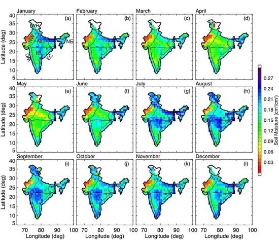
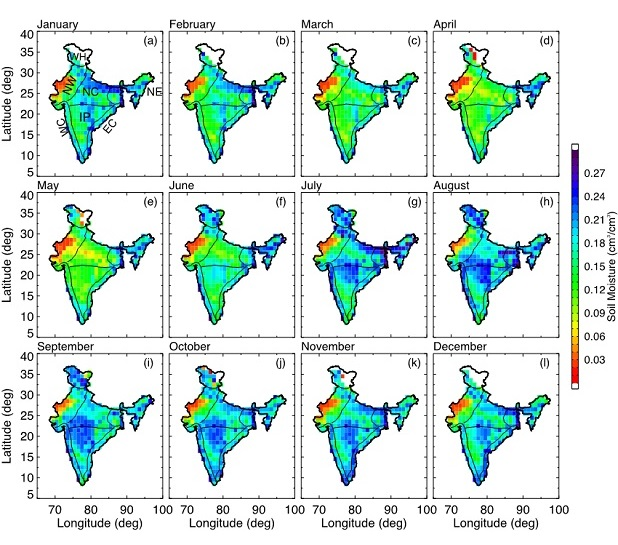
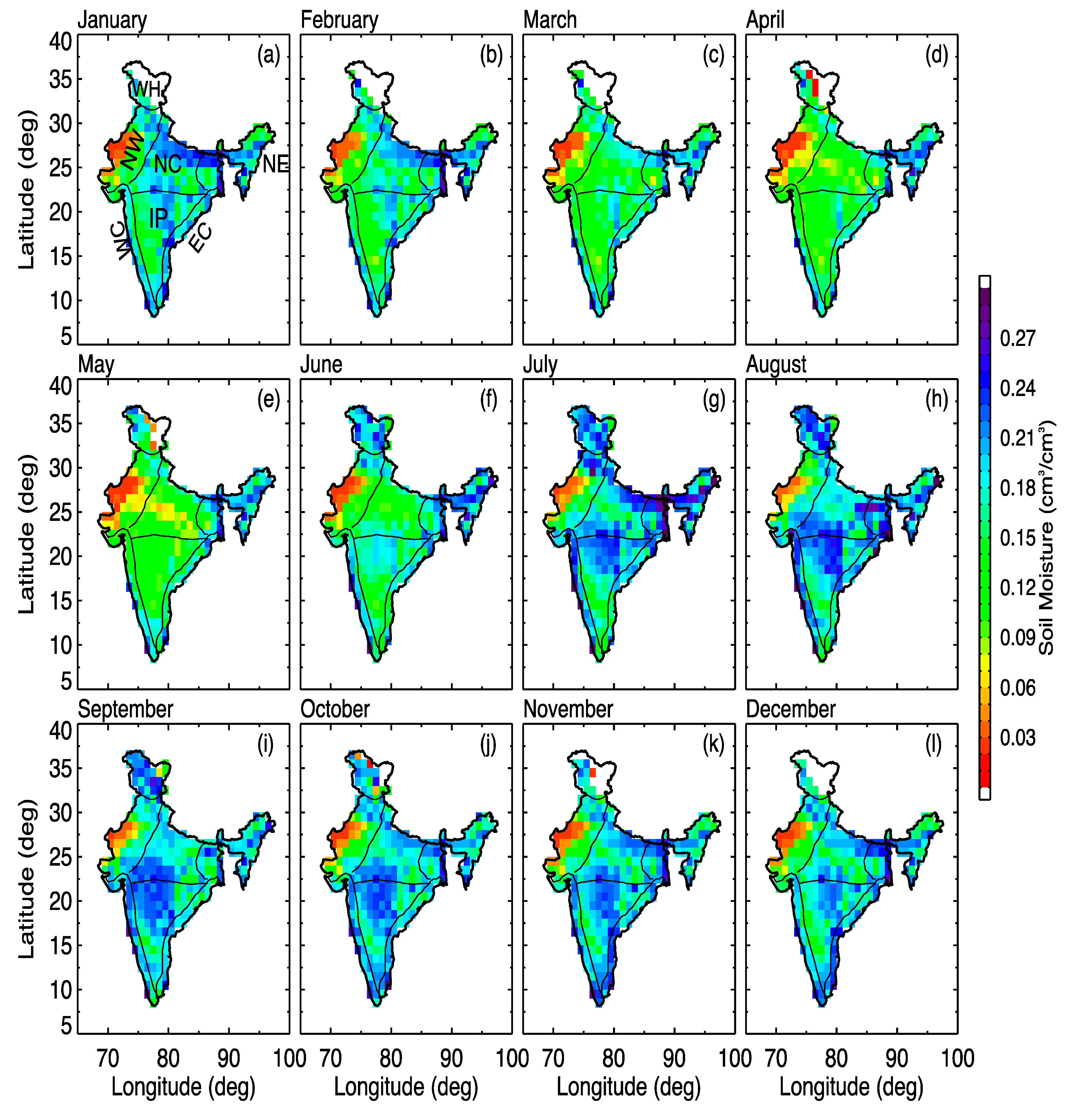
4.1. Spatial Monthly Variability of Soil Moisture

Figure 1 shows the spatial monthly variations of AMSR soil moisture during the period from June 2002 to April 2017. North central and interior peninsula regions show the highest soil moisture over monsoon (June - September) and post-monsoon (October and November) months. The majority of months with lower soil moisture are mainly found over the northwest region of India. Note that insufficient observations are available over the Himalayan region during winter and pre-monsoon months. The spatial distribution of soil moisture shows a similar behavior in March and April as well as in November and December. Over the interior peninsula and north central regions, AMSRSM values are ~70% larger than in other regions. The large SM may largely be attributed to monsoon precipitation and advection of moisture from neighboring regions. Anusha et al. [43] mentioned the larger SM over central regions of India using one year of summer soil moisture data. Figure 1 clearly shows the seasonal variation of soil moisture, which is an input to the agricultural production of the country.

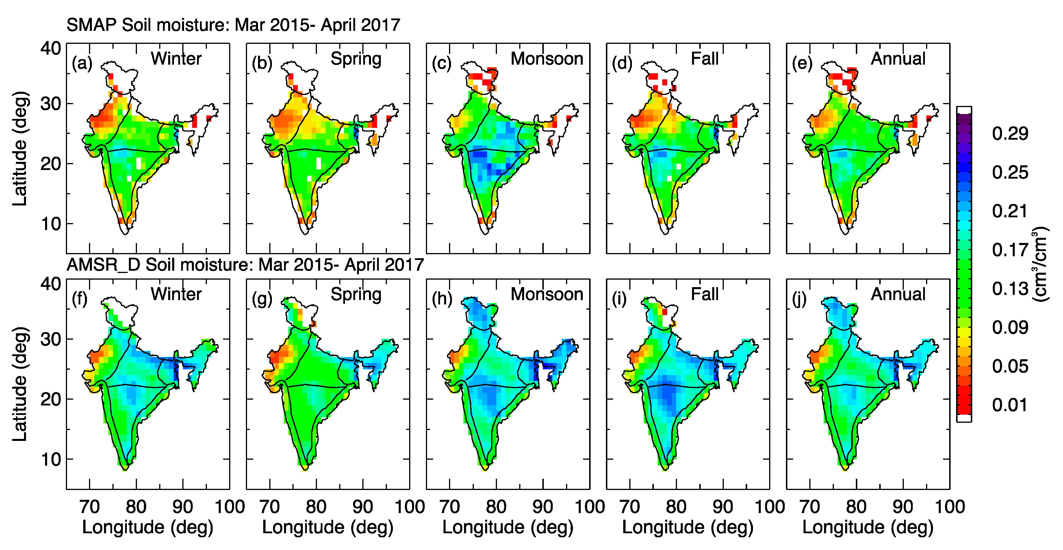
4.2. Seasonal and Annual Gridded Soil Moisture

The spatial distribution pattern of annual and seasonal soil moisture, and relative difference of soil moisture over India are discussed in this section. The seasonal and annual soil moisture variations of SMAP (top panel) and AMSR (bottom panel) are shown in Figure 2. For an equal comparison, SMAPSM and AMSRSM data were used only within the period of March 2015–April 2017. The seasonal means refer to the following months: winter (December, January, and February), pre-monsoon (March–May), monsoon (June-September), and post-monsoon (October and November). In all seasons, the minimum soil moisture (<0.02 cm3/cm3) values are in the northwestern (NW) region. SMAP shows relatively drier conditions than AMSRSM in winter, especially over northwest, north central, and interior peninsula regions. In the spring season, both SMAP and AMSR report drier soil moisture conditions over the northwest, extending further to the north central region. During monsoon and fall seasons, there is relatively more soil moisture over north central and Interior peninsula regions in both satellite measurements. The maximum values of soil moisture over central and Interior Peninsula regions are observed during monsoon season. The monthly soil moisture distribution in these regions tends to increase from June to November and then decrease gradually from December to March, with the minimum being in May. Unnikrishnan et al. [44] also observed maximum soil moisture during monsoon season over central India using United Kingdom meteorological Office (UKMO) datasets. The annual mean soil moisture is comparable in both datasets, with the exception of the Western Himalayas region. These seasonal trends are important because an increase (decrease) in food grain yield is associated with an increase (decrease) in soil moisture.
The annual and seasonal behavior of the AMSR and SMAP soil moisture are shown in Figure 2. AMSR shows higher soil moisture values than SMAP over northwest and north central regions of India in winter, spring, and fall, as well as the annual period. In the monsoon season, AMSRSR is lower (drier) than SMAP in all regions over India except for the Himalayas, since AMSRSR is more sensitive to the very top layer. During the monsoon and fall seasons, AMSRSM is higher over North central and Interior peninsula regions, whereas SMAP shows maximum soil moisture values in the monsoon season but not in the fall season. It is evident from Table 1 that in the Northeast (NE) the mean monsoon soil moisture is highest in AMSR followed by that in SMAP. Furthermore, SMAP and AMSR display the strongest intra-seasonal variation of soil moisture over central India. In the monsoon season, the SMAP maximum and minimum seasonal mean value is observed in the Interior peninsula (IP) and Western Himalaya (WH), respectively. Meanwhile, AMSR has a minimum value of 0.10 cm3/cm3 in the Northwest (NW) during spring and a maximum value of 0.22 cm3/cm3 in the Northeast (NE) during the monsoon season. In general, the annual regional means of soil moisture from AMSR and SMAP show general agreement, with the mean values ranging from 0.13 to 0.20 cm3/cm3 and 0.10 to 0.16 cm3/cm3, respectively.

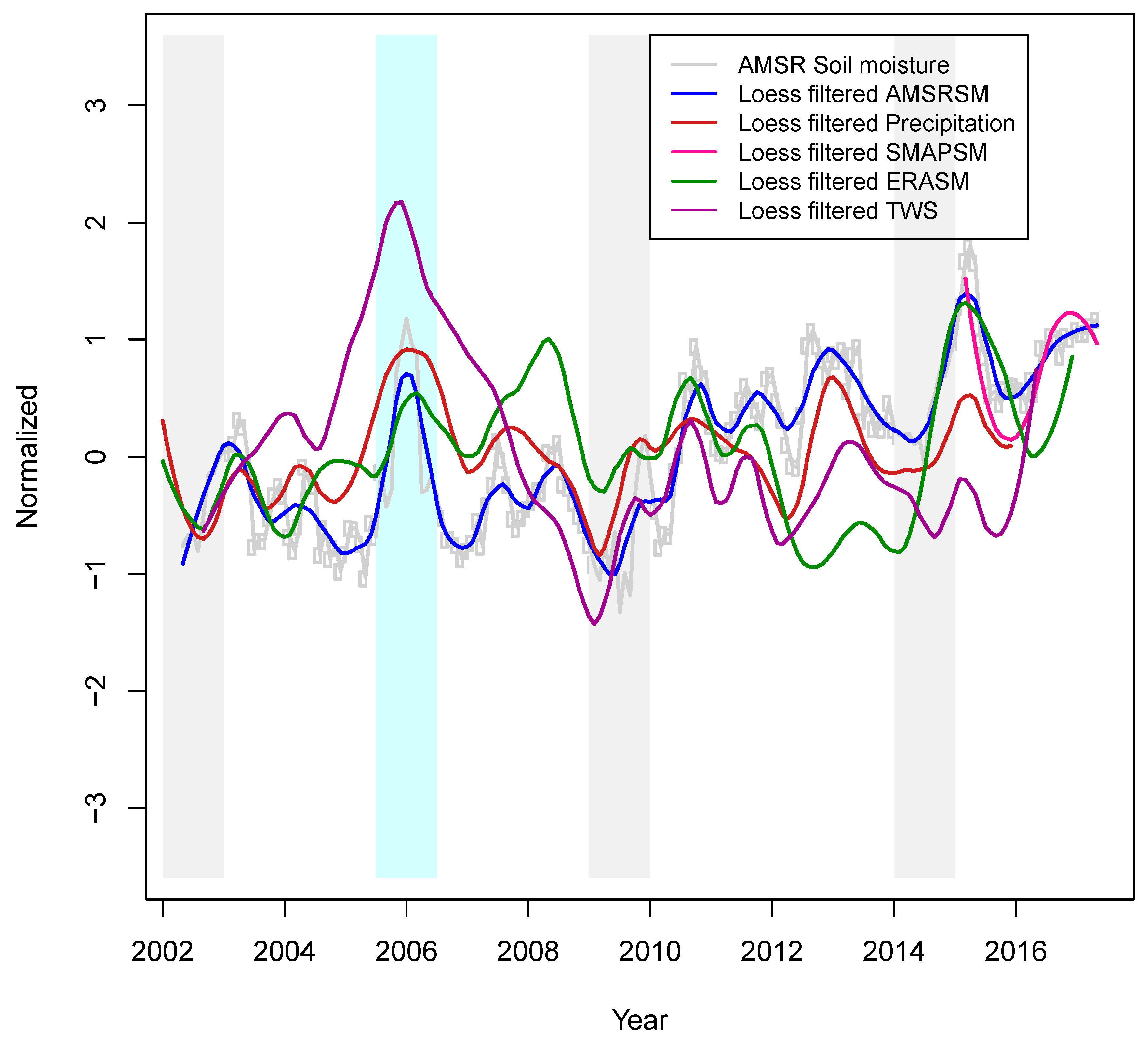
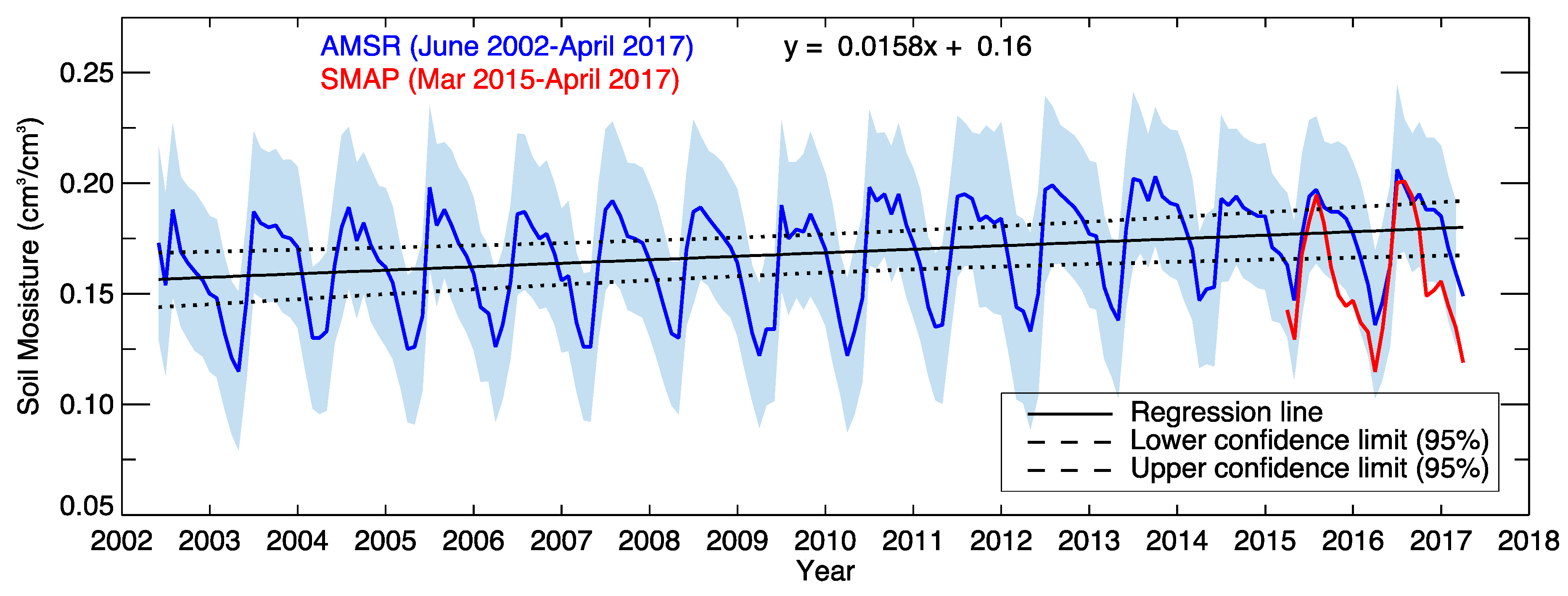
4.3. Interannual Variability of Soil Moisture

The year-to-year variations of soil moisture, precipitation, and TWS in India are shown in Figure 3. Normalized values were estimated by subtracting monthly soil moisture values from the long-term climatology calculated from averaging the monthly values over India, and by dividing by the monthly standard deviation. The AMSR soil moisture time series is shown by a gray color with open circles, but it also contains locally estimated scatterplot smoothing (LOESS) curves (smoothing parameter α=0.75) also plotted in Figure 3. The LOESS smoothing technique based on locally weighted regression smoothing [45]. The time series exhibit consistent year-to-year and seasonal variability, and the nature of the intra-seasonal variability looks similar during periods of major droughts or major floods [46]. On the other hand, two dominant intra-seasonal oscillatory modes and large-scale standing patterns are observed using outgoing longwave radiation (OLR) datasets [47]: one at the equatorial Pacific and the other over the equatorial Indian Ocean. Spatial and temporal variations of rainfall influence the spatiotemporal distribution of runoff, soil moisture, and groundwater reserves, which in turn affect the frequency of droughts and floods. Ultimately, these drought and floods affect the patterns of vegetation productivity in India.
The normalized plot (Figure 3) shows variations in soil moisture during the period of 2002 to 2016. Both SMAP and AMSR records show consistent variability during the overlapping period. Before the SMAP record started, there were the three major droughts shown by the vertical gray bars in Figure 3, in 2002, 2009, and 2014. The year 2009 and 2002 had the third and fourth largest major droughts in the past 100 years, after 1918 and 1972. In contrast to the AMSR record, the ERA-Interim reanalysis soil moisture estimate did not capture the year 2009 drought. Neena et al. [48] also mentioned the failure of global models in the 2009 severe drought, when a seasonal rainfall deficit of 21.5% in 2002 and ~24% was recorded [49]. In addition, the AMSR SM record also successfully captured the extreme flooding events from 2005–2006 [49].

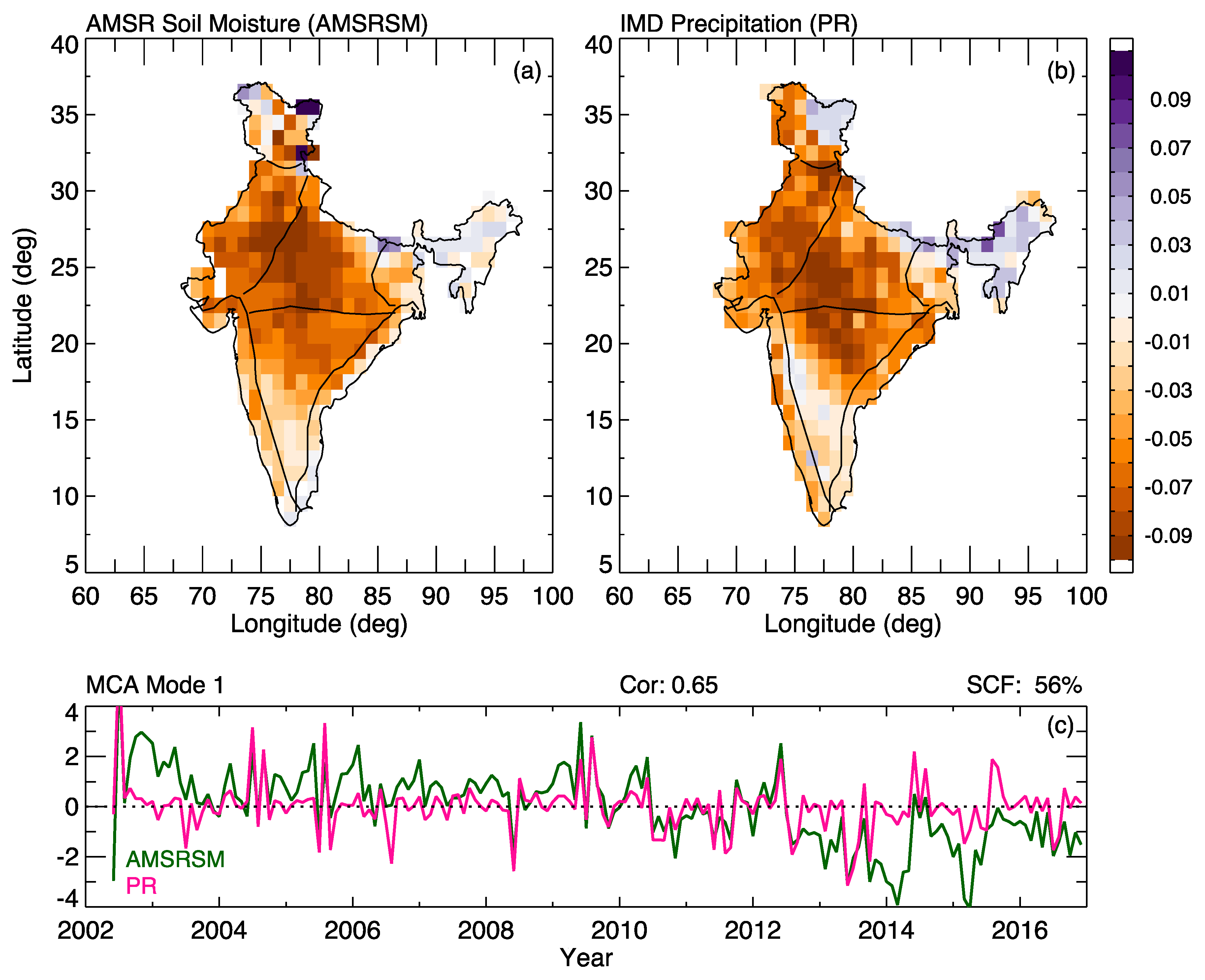
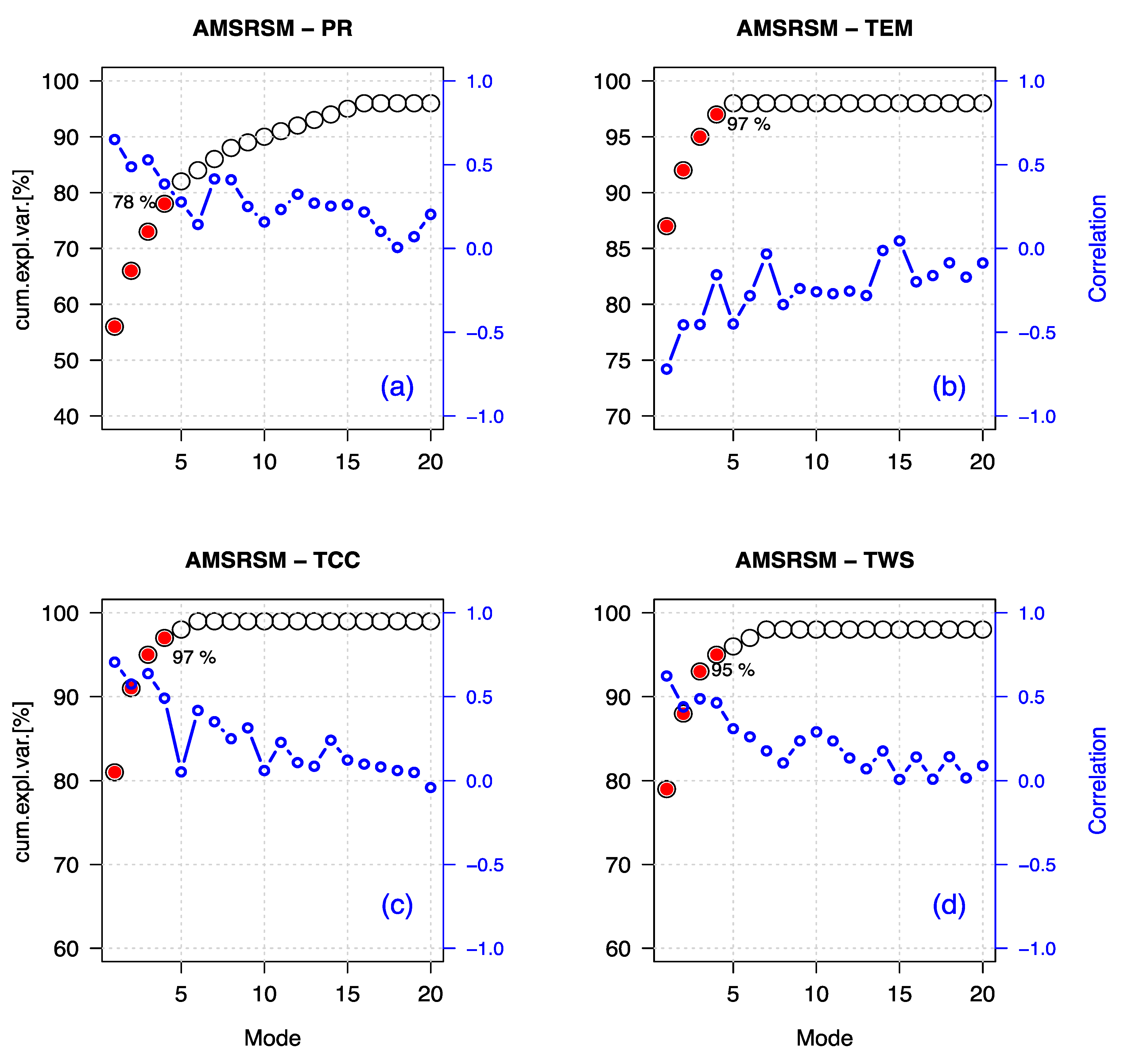
4.4. Soil Moisture–Precipitation (SM–PR) MCA Results

Here, Maximum Covariance Analysis (MCA) was used to investigate the spatiotemporal relationship of the covariance between SM and precipitation datasets. Figure 4a,b show the first mode of maximum covariance patterns of precipitation and soil moisture for 2002–2016. Here, the monthly spatial anomalies of precipitation and soil moisture data were utilized. The first mode shows similar general patterns in the northwest, north central, and northern parts of the Interior Peninsula. Over the Northeast, precipitation patterns resemble those of soil moisture. Both variables exhibit the opposite sign in the Western Himalayas compared to the northeast, which is the main driving force of SM change. Note that the precipitation datasets have less coverage over the Western Himalayas. A squared covariance factor (SCF) of 56% (see Figure 4c) is observed between two fields, indicating the large-scale coupling between soil moisture and precipitation monthly anomalies. In the temporal domain, these time series datasets are strongly correlated (r = 0.62), which indicates a strong association between SM and PR, both of which exhibiting a slight downward trend since 2010 (Figure 4c). It can be seen in Figure 4c that soil moisture and precipitation demonstrate a strong seasonal cycle and coupling in India, as most rainfall occurs during the monsoon season in central India. These findings are consistent with previous observations and model simulations. For instance, Jung et al. [50] observed a significant negative trend over the global tropics (28°S–38°N) using soil moisture and evapotranspiration data. Douville et al. [51] studied model-derived soil moisture over Asia and Africa, concluding that surface wetness in India contributes to increased rainfall. Later, Orlowsky and Senevirante [52] found remarkable coupling strength between soil moisture and precipitation for specific regions.

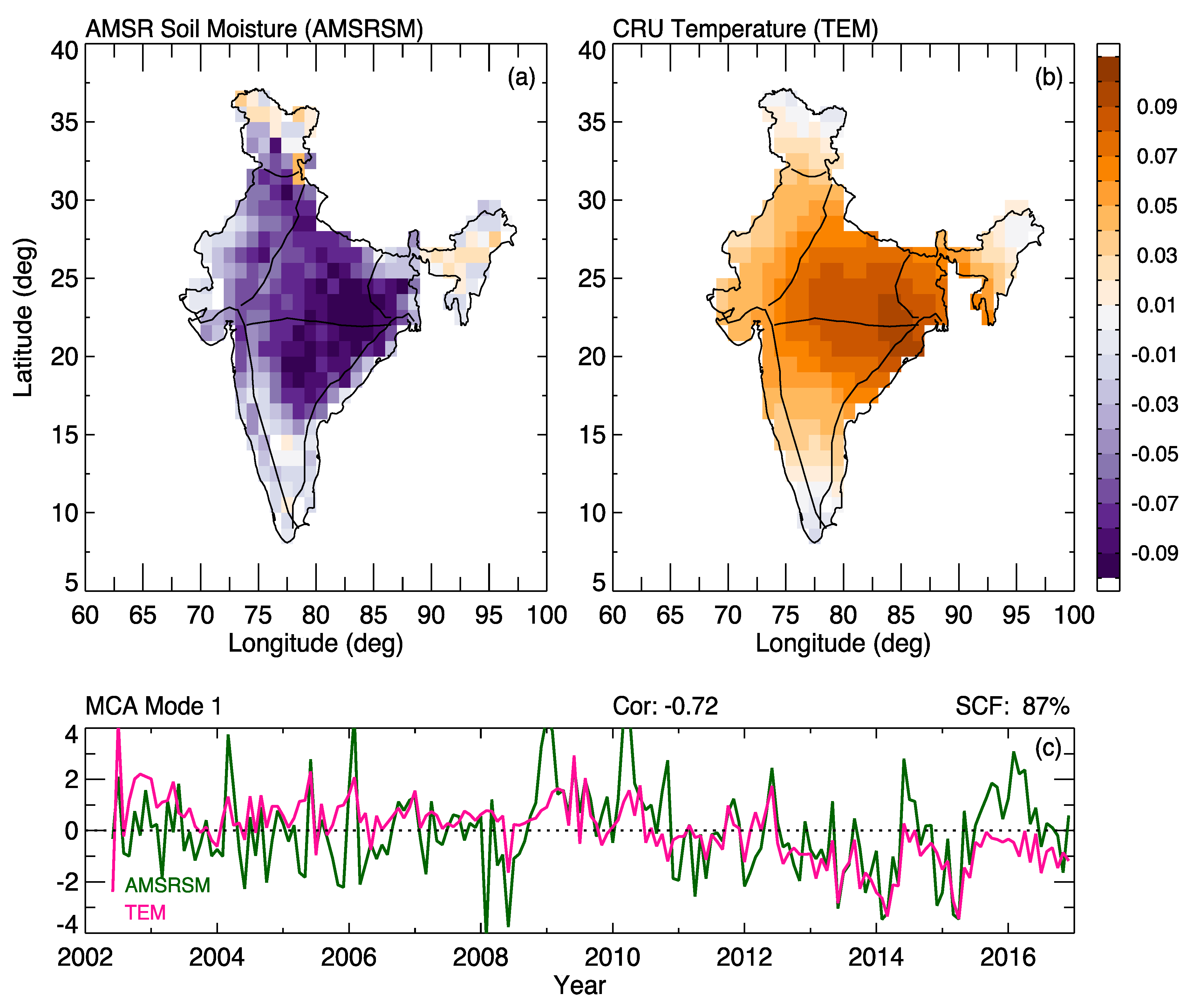
4.5. Local Temperature Impact on Soil Moisture (SM–TEM)

To investigate how the spatial pattern of the surface temperature in India is affected by soil moisture, we once again utilized MCA during the period 2006 to 2016. The covariance analysis was applied after removing the long-term trends from both the datasets, the results of which are shown in Figure 5. The soil moisture pattern reveals more variability over the northeastern central and northeastern Interior Peninsula regions, which shows strong anti-correlation with temperature. A positive temperature anomaly is observed over the eastern part of India, concurrent with negative soil moisture anomalies in the same region. Higher temperatures can lead to a greater potential evaporation over land, resulting in a declining soil moisture. Furthermore, warm temperatures frequently accompany the shortage of rainfall, leading to agricultural droughts that are normally associated with soil moisture deficiency. Recent studies with CRU temperature and CMIP5 simulations also indicate that central and northeastern regions show the highest warming compared with the other regions [53]. The first mode of MCA explores the largest variability between soil moisture and TEM. The total amount of variance of the first mode reaches 28% for soil moisture and 42% for temperature. The squared covariance factor of 87% between the two fields is illustrated in Figure 5c. The correlation between the two time series is about −0.72, which is significant at the 95% level. MCA analysis indicates an inverse relationship between SM and TEM variance; the higher the TEM variance, the lower the SM variance. Note that the time series show similar patterns, with a decreasing trend from 2008 to 2014. It indicates that temperature controls the evapotranspiration and consequently affects the soil moisture. Our results for SM couplings with PR and TEM suggest that temperature has a larger contribution than precipitation to soil moisture variation in India, consistent with previous study in a similar humid basin environment [54]. The inverse relationship indicates that a decrease in soil moisture may be responsible for an increase in temperature. This conclusion is generally true in most regions, with some exceptions that exhibit complicated soil moisture–climate interaction and feedback.

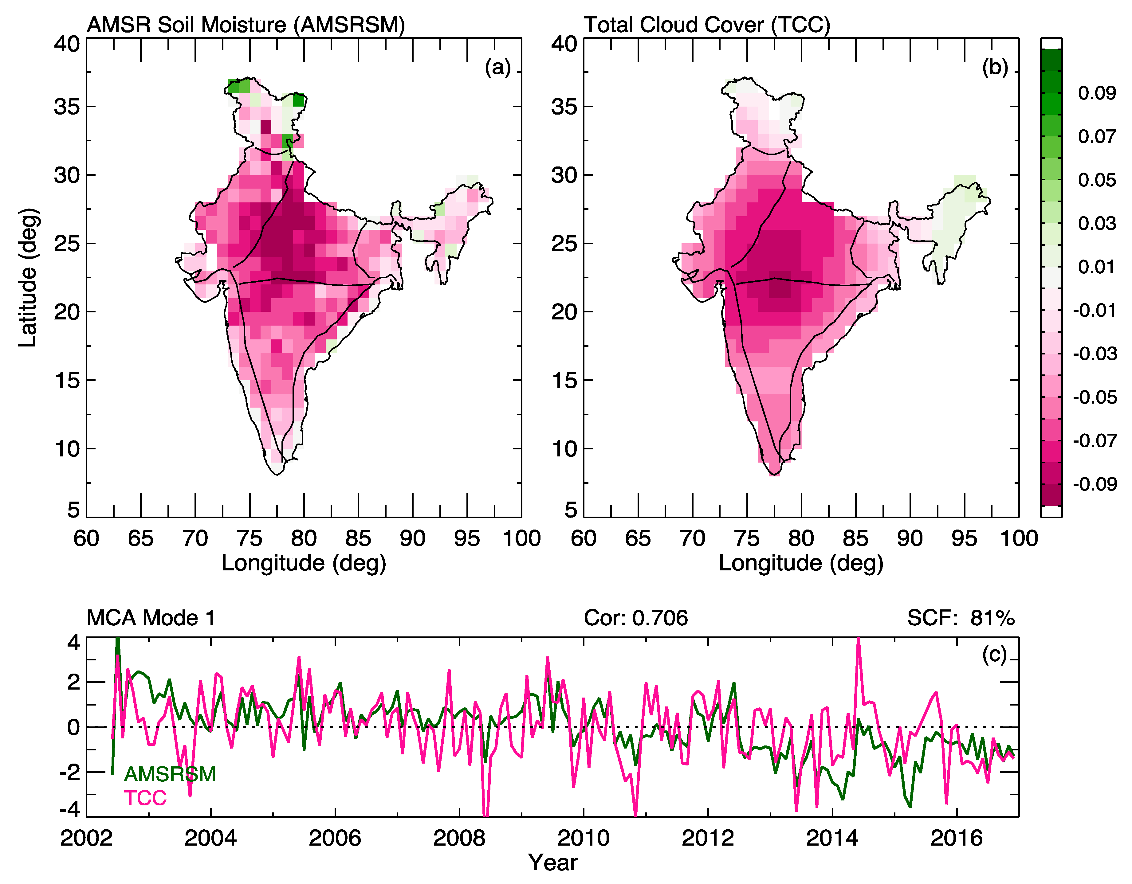
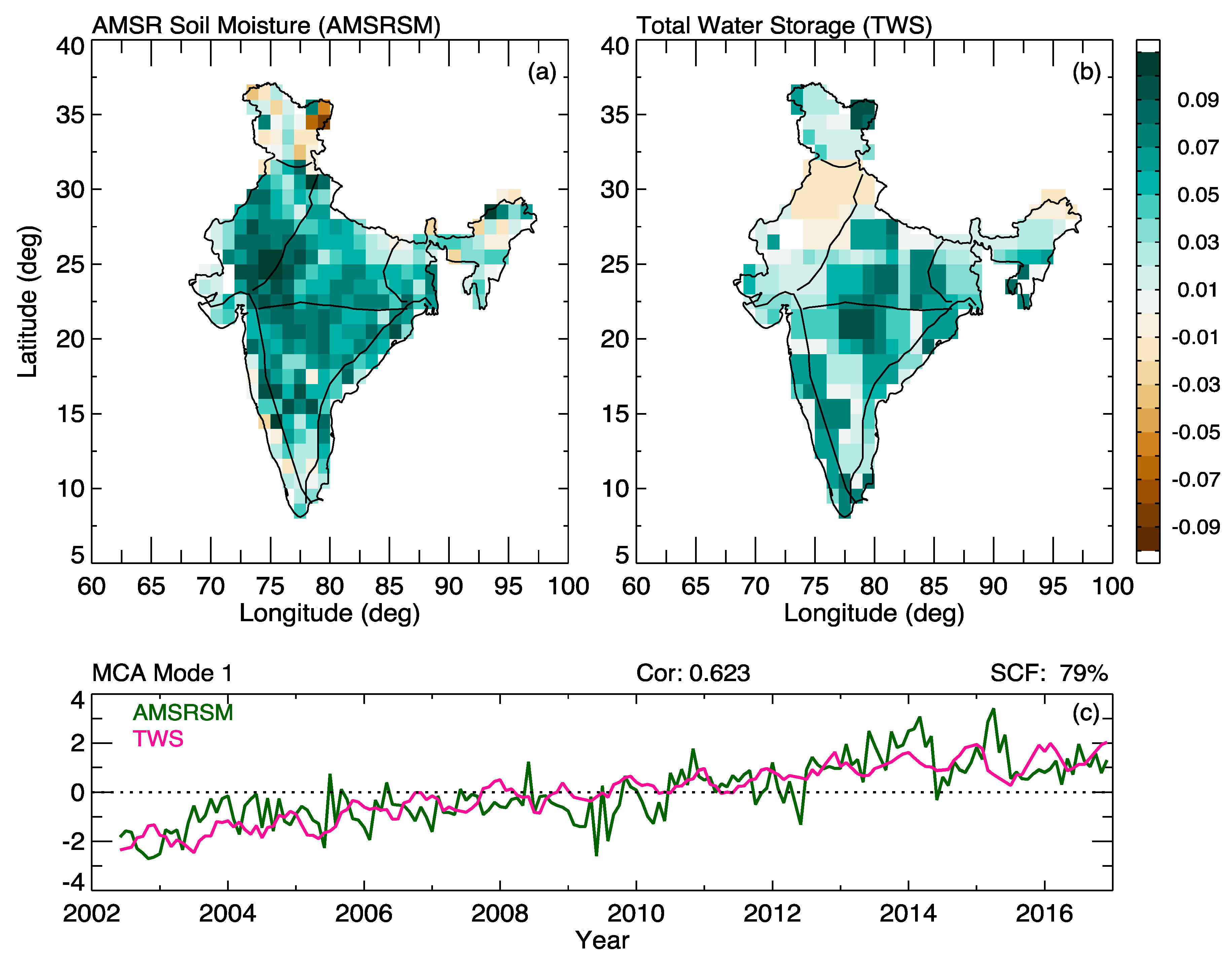
4.6. Relation Between TCC, TWS and SM

Figure 6 and Figure 7 show the first leading modes of covariance between SM and TCC, and SM and TWS for the period of 2006–2016. In Figure 6, the SM pattern tends to be zonally elongated from the Northwest to the Interior Peninsula. The SM covariance anomalies match those of TCC. The maximum variance of SM concentrated over central India is closely associated with total cloud events in that region (Figure 6a,b), which shows a strong similarity between the two variables. It suggests that a large increase in cloud cover can reduce the surface air temperature and increase the soil moisture. The SCF between SM and TCC is about 81%. The time series of AMSRSM and TCC show clear decreasing trends. The decreasing trends may be linked to ENSO (El Nino Southern Oscillation) variation. However, TCC feedback remains a source of uncertainly in global climate change Intergovernmental Panel on Climate Change (IPCC 2007 [55]). Rao et al. [56] observed decreasing trends in total cloud cover in many regions throughout India from 1951 to 2000. TCC and TWS variability has a statistically significant impact on SM over several regions in India. It is clear that the higher correlations, the bigger the influence of TCC on evapotranspiration; indeed, the highest values can be found in monsoon and post-monsoon followed by the winter and summer. About 60% of the world is covered by clouds, and the influence of clouds on both the water balance and global radiation budget, even small variations, can alter the climate response [57,58]. The spatial patterns of variance for SM and TWS are consistent, with the exception of the northwest, northeast, and west coast regions, where TWS shows negative variances but where SM still has positive variances. The first mode of MCA yields a squared covariance factor of about 79% between the SM and TWS. The time series of SM and TWS show significant increasing trends with a positive correlation of about 0.62, suggesting that the soil moisture variability is the main driver of the regional change in the water balance. TWS changes reflect the balance or imbalance of water fluxes (precipitation, evapotranspiration, and runoff) and are strongly affected by regional climate conditions. Furthermore, the interannual and decadal climate variability caused by large-scale ocean–atmosphere interactions might influence moisture advection, rainfall, and eventually TWS changes at long-term timescales [59].
The cumulative SCF across MCA modes from SM and PR, TEM, TCC, and TWS as well as the correlation between the time series obtained from each mode are shown in Figure 8. The first two leading modes account for most of the variation, which account for 56%, 10% (PR), 87%, 5% (TEM), 81%, 10% (TCC), and 79%, 9% (TWS) of the SCF, respectively. Significance levels were estimated at each mode using a moving block bootstrap procedure as described by Wilks [57]. The significant modes are shaded in red in Figure 8. The SCF explained by the first four modes exceeds 95% significance.
The four leading modes explain about 97%, 97%, 78%, and 95% of the SCF for SM–TCC, SM–TEM, SM–PR, and SM–TWS, respectively. The rest of the MCA modes only explain approximately 5% of the squared covariance, with the exception of SM–PR modes. The first four leading modes represent the major characteristics of SM and other fields (PR, TEM, TCC, and TWS) in India. The correlation coefficients between AMSRSM and the variables are 0.65 (PR), −0.72 (TEM), 0.71 (TCC), and 0.62 (TWS) for the first leading mode. The correlation coefficients decrease as the mode increase, which indicates a teleconnection between SM–PR, SM–TWS and SM–TCC. There is an anti-correlation with surface temperature. SM is indirectly related to the surface temperature, because increasing surface temperatures leads to a decreasing soil moisture due to evaporation.

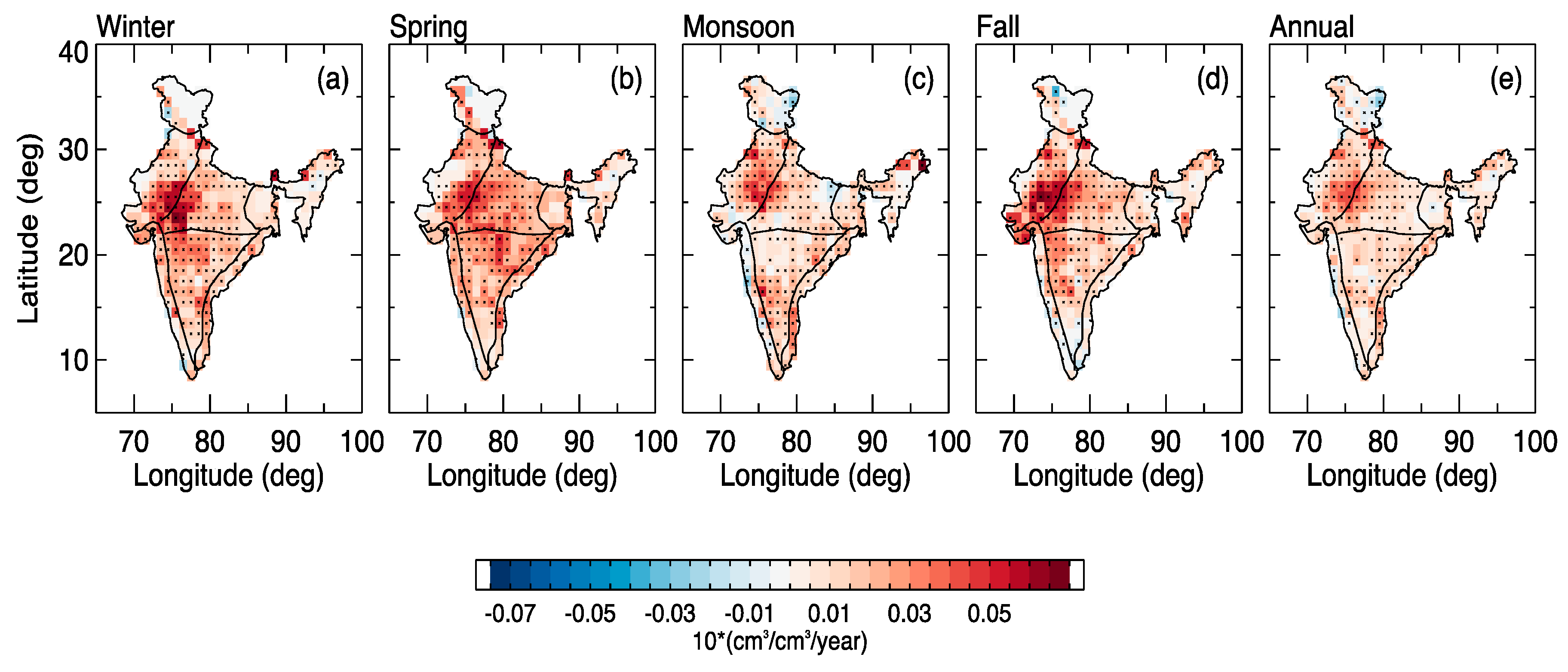
4.7. Spatial Soil Moisture Trends

Next, seasonal (a–d) and annual (e) SM trends were analyzed, with the results shown in Figure 9. Robust regression analysis was utilized to obtain the seasonal and annual SM trends for each grid cell throughout India during the period from June 2002 to April 2017. The statistical significance of the trends was calculated by using the Monte Carlo test as described in Allen and Smith [58] and marked as asterisks where the trends are statistically significant at the 95% confidence level. In all seasons, there is an increasing SM trend in most regions. Seasonal SM exhibits a positive trend, which is particularly pronounced in the northwestern region, and a moderate trend in several other regions. However, decreasing trends (−0.01 to −0.025 cm3/cm3 per decade) appear in the Western Himalayas and southern India. Therefore, there is clear evidence that there are large precipitation variations, especially in north central and interior peninsula regions due to monsoon rainfall. The decreasing trends may be due to the southeastern monsoon. The rainfall is high over the eastern part and decreases northwestward across the zone and near the northwestern boundary. As the monsoon continues, the air moisture content is reduced and the monsoon precipitation gradually decreases from east to west [60]. The central part of India is characterized by the presence of a large area with positive SM trends that are statistically significant (95%) over winter, spring, and fall seasons. The positive trends vary between 0.03 to 0.05 cm3/cm3 per decade.
The fact that increasing or decreasing soil moisture trends may have an adverse effect on food grain yield points towards the existence of a potentially linear or nonlinear relationship between SM and better food grain yield. Rajeevan and Nayak [59] have reported increasing trends in annual mean soil moisture in 15 out of 27 stations in India during the period of 1991–2013. There were significantly increasing trends in north, central, and northeast India as well as on the west coast. They stated that in situ SM datasets are costly, labor intensive, and not extensively quality-controlled. Nevertheless, relative surface atmospheric moisture studies in India conducted by Jaswal and Koppar [61] have also reported significantly increasing trends of specific humidity during summer and winter as well as annual time frames, especially over northwest, central, and southeast regions of India. Rajeevan and Nayak [59] found positive soil moisture trends over 15 different meteorological stations in India during the period 1991–2012.
Figure 10 shows the monthly variations and the linear trend of the AMSR and SMAP soil moisture in Indian for the periods June 2002–April 2017 and Mar 2015–April 2017. The monthly means in the figure clearly show the interannual variability of AMSR soil moisture. It is noteworthy that the monthly SM time series of AMSR and SMAP are correlated with each other, although they exhibit some small differences in their year-to-year variability. The monthly mean values across all of India have a moderate standard deviation ranging from -0.085 to 0.20 cm3/cm3 towards the end of the observation. The blue-shaded region indicates the internal regional variability of the soil moisture. The maximum standard deviation is seen August and September, indicating a high degree of uncertainty, which may be due to the year to year variation of summer monsoon. The results show a positive trend of 0.016 cm3/cm3 per decade for the entire period of AMSR observations for all of India. The more positive trends are found in the northwest and north central regions.

5. Conclusions

This study explored the spatial distribution, characteristics, and temporal variability of soil moisture on monthly, seasonal, and annual temporal scales using AMSR and SMAP satellite observations. The spatiotemporal coherency between soil moisture and geophysical fields (PR, TEM, TCC, and TWS) were examined using the powerful tool of Maximum Covariance Analysis (MCA). In addition, trends were estimated using robust regression with a 95% confidence level for annual and seasonal (winter, spring, monsoon, and fall) time frames. The trends indicate the increase or decrease of soil moisture in India on regional scales, which are essential for a better understanding of agricultural yields. The most important findings of our analysis are summarized as follows:
Firstly, the characteristics of satellite-observed soil moisture in India were presented using 15 years of data. The mean seasonal soil moisture from AMSR shows a maximum value of about 0.22 cm3/cm3 over the northeast region followed by the East Coast (0.21 cm3/cm3). The monthly mean values of AMSR and SMAP soil moisture show a reasonably good agreement. However, the spatial distributions of annual and seasonal soil moisture show some discrepancies between AMSR and SMAP in some regions (West Coast and Western Himalayas). The relative SM difference over the seven regions in India shows that AMSR is higher than SMAP over the east coast in winter (20.41%), but lower over the Interior Peninsula in the monsoon season (−7.34%).
The normalized time series of different observations (SM, TWS, and PR) all clearly show drought years in 2002, 2009, and 2014, as well as an excess of water in the year 2006. The MCA method is a powerful technique that identifies spatial patterns of maximum covariance between two fields. These results indicate that the spatial and temporal patterns of SM and surface–atmosphere fields (PR, TEM, TCC, and TWS) agree well. The first MCA mode explains about 56%, 87%, 81%, and 79% of the squared covariance between SM–PR, SM–TEM, SM–TCC, and SM–TWS, respectively, with the corresponding time series having correlation coefficients of 0.65, −0.72, 0.71, and 0.62. These results indicate strong teleconnection patterns associated with soil moisture and land surface–atmosphere parameters.
The annual and seasonal trends were computed at each grid cell (1° × 1°) for the period June 2002–April 2017. It is worth mentioning here that the positive trends are obtained for most regions on annual and seasonal scales (for all seasons) throughout India. The hilly regions, both in the northeast and the west coast of India, all exhibit small negative trends, but these are only in small regions in northern and southern parts of India. The regional moisture budget shows that changes in precipitable water and precipitation efficiency vary temporally and spatially in India. The maximum positive trend occurs in the northwest and north central regions of India in all seasons. Moderate positive trends for the annual scale are observed over northwest and north central regions. In addition, the trends were estimated using monthly means of soil moisture throughout India, revealing an increasing trend of about 0.0158 cm3/cm3 per dec from 2002 to 2017. The outcomes acquired in this trend analysis provide evidence of significant overall increase in SM content throughout India. Positive trends in SM indicate favorability for irrigation. However, some regions show small SM trends, which are more useful for single-cropping. The two crop-growing seasons, the Kharif (May–October) and the Rabi (October–April) were identified to have a high importance for agricultural production in India. In the Rabi period, increased temperatures may have profound implications for crop yields as well as fewer requirements for irrigation, especially in northwestern India [8]. This research is directly applicable to seasonal water management for accounting the water budgets (recharge, runoff, evapotranspiration). Understanding the changes and variability in runoff, evapotranspiration, precipitation, and soil moisture under retrospective and projected climate in the key crop-growing seasons is of utmost importance.
These satellite measurements provide valuable insights into the spatial and temporal characteristics of soil moisture in India, given the parse nature of ground-based measurements. Long-term observations of regional characteristics are beneficial for a better understanding of crop cultivation and agricultural yield, and ultimately boosting the economy of the country. High-resolution datasets of soil moisture are crucial for a better understanding of the future across various regions of India.

Author Contributions

Data curation, G.A., E.C., S.C., G.B. and S.V.B.R.; Funding acquisition, I.V.; Writing—original draft, and analysis, K.P.; Writing—review & editing, Y.M.

Acknowledgments

We acknowledge all groups who contributed the datasets that supported this work. The standard AMSR-2 soil moisture was obtained from NASA (Goddard Earth Sciences Data Information Services Center) data archive. Authors also wish to thank the ECMWF, SMAP, IMD, and CRU people for providing the datasets. We also thank the JPL team for providing their GRACE datasets.

Conflicts of Interest

The authors declare no conflict of interest.

References

  1. Seneviratne, S.I.; Corti, T.; Davin, E.L.; Hirschi, M.; Jaeger, E.B.; Lehner, I.; Orlowsky, B.; Teuling, A.J. Investigating soil moisture climate interactions in a changing climate: A review. Earth Sci. Rev. 2010, 99, 125–161. [Google Scholar] [CrossRef]
  2. GCOS-138. Implementation Plan for the Global Observing System for Climate in support of the UNFCCC-2010 Update; World Meteorological Organization: Geneva, Switzerland, 2010. [Google Scholar]
  3. Koster, R.D.; Suarez, M.J. The relative contributions of land and ocean processes to precipitation variability. J. Geophys. Res. 1995, 100, 13775–13790. [Google Scholar] [CrossRef]
  4. Liu, Y. Prediction of monthly-seasonal precipitation using coupled SVD patterns between soil moisture and subsequent precipitation. Geophys. Res. Lett. 2003, 30, 1827. [Google Scholar] [CrossRef]
  5. Jiang, Y.; Fu, P.; Weng, Q. Assessing the impacts of Urbanization-associated land use/cover change on land surface temperature and surface moisture. Remote Sens. 2015, 7, 4880–4898. [Google Scholar] [CrossRef]
  6. Huang, J.; van den Dool, H.M.; Georgakakos, P.K. Analysis of model calculated soil moisture over the United States (1991–1993) and applications to long-rangetemperature forecasts. J. Clim. 1996, 9, 1350–1362. [Google Scholar] [CrossRef]
  7. Wang, W.Q.; Kumar, A. A GCM assessment of atmospheric seasonal predictability associated with soil moisture anomalies over North America. J. Geophys. Res. 1998, 103, 28637–28646. [Google Scholar] [CrossRef]
  8. Mishra, V.; Shah, R.; Thrasher, B. Soil moisture droughts under the retrospective and projected climate in India. J. Hydrometeorol. 2014. [Google Scholar] [CrossRef]
  9. Shukla, J.; Mintz, Y. Influence of land-surface evapotranspiration on the Earth’s climate. Science 2015, 215, 1498–1501. [Google Scholar] [CrossRef]
  10. Asharaf, S.; Dobler, A.; Ahrens, B. Soil moisture-precipitation feedback processes in the Indian summer monsoon season. J. Hydrometoerology 2012. [Google Scholar] [CrossRef]
  11. Verikoden, H.; Revadekar, J.V. Relation between the rainfall and soil moisture during different phases of Indian monsoon. Pure Appl. Geophys. 2018, 175, 1187–1196. [Google Scholar] [CrossRef]
  12. Kantharao, B.; Rakesh, V. Observational evidence for the relationship between spring soil moisture and June rainfall over the Indian region. Theor. Appl. Climatol. 2018, 132, 835–849. [Google Scholar] [CrossRef]
  13. Raman, S.; Mohanty, U.C.; Reddy, N.C.; Alpaty, K.; Madala, R.V. Numerical simulation of the sensitivity of summer monsoon circulation and rainfall over India to land-surface processes. Pure Appl. Geophys. 1998, 152, 781–809. [Google Scholar] [CrossRef]
  14. Dirmeyer, P.A.; Dolman, J.; Sato, N. The pilot phase of the Global Soil Witness Project. Bull. Am. Meteorol. Soc. 1999, 80, 851–878. [Google Scholar] [CrossRef]
  15. Koster, R.D.; Dirmeyer, P.A.; Guo, Z.; Bonan, G.; Chan, E.; Cox, P.; Gordon, C.T.; Kanae, S.; Kowalczyk, E.; Lawrence, D.; et al. Regions of strong coupling between soil moisture and precipitation. Science 2004, 305, 1138–1140. [Google Scholar] [CrossRef] [PubMed]
  16. Dorigo, W.; de Jeu, R.; Chung, D.; Parinussa, R.; Liu, Y.; Wagner, W.; Fernandez-Prieto, D. Evaluating global trends (1998–2010) in harmonized multi-satellite surface soil moisture. Geophys. Res. Lett. 2012, 39, L18405. [Google Scholar] [CrossRef]
  17. Pariussa, R.M.; de Jeu, R.A.M.; van der Schalie, R.; Crow, W.T.; Lei, F.; Holmes, T.R.H. A Quasi-Global approach to improve day-time satellite surface soil moisture anomalies through the land surface temperature input. Climate 2016, 4, 50. [Google Scholar] [CrossRef]
  18. Liu, Y.; Zhao, W.; Wang, L.; Zhang, X.; Daryanto, S.; Fang, X. Spatial variations of soil moisture under Caragana Korshinskii Korn from different precipitation zones: Field based analysis in the Loess Plateau, China. Forests 2016, 7, 31. [Google Scholar] [CrossRef]
  19. Tiwari, V.M.; Wahr, J.; Swenson, J. Dwindling groundwater resources in northern India, from satellite gravity observations. Geo. Phys. Res. Lett. 2009, 36, L18401. [Google Scholar] [CrossRef]
  20. Njoku, E.G.; Chan, S.K. Vegetation and surface roughness effects on AMSR-E land observations. Rem. Sen. Environ. 2006, 100, 190–199. [Google Scholar] [CrossRef]
  21. Owe, M.; De Jeu, R.A.M.; Holmes, T.R.H. Multi-sensor historical climatology of satellite-derived global land surface moisture. J. Geophys. Res. 2008, 113, R01002. [Google Scholar] [CrossRef]
  22. Jones, L.A. Synthesis of Satellite Microwave Observations for Monitoring Global Land-Atmosphere CO2 Exchange. Ph.D. Thesis, College of Forestry and Conservation, Missoula, MT, USA, 2016. [Google Scholar]
  23. Du, J.; Kimball, J.S.; Jones, L.A.; Kim, Y.; Glassy, J.; Watts, J.D. A global satellite environmental data record derived from AMSR-E and AMSR2 microwave Earth observations. Earth Syst. Sci. 2017, 9, 791–808. [Google Scholar] [CrossRef]
  24. Entekhabi, D.; Njoku, E.G.; O’Neill, P.E.; Kelogg, K.H.; Crow, W.T.; Edelstein, W.N.; Entin, J.K.; Goodman, S.D.; Jackson, T.J.; Johnson, J.; et al. The Soil Moisture Active Passive (SMAP) mission. Proc. IEEE 2010, 98, 704–716. [Google Scholar] [CrossRef]
  25. Pan, M.; Cai, X.; Chaney, N.W.; Wood, E.F. An initial assessment of SMAP soil moisture retrievals using high-resolution model simulations and in situ observations. Geophys. Res. Lett. 2016. [Google Scholar] [CrossRef]
  26. Zeng, J.; Chen, K.S.; Chen, Q. A preliminary evaluation of the SMAP radiometer soil moisture product over United States and Europe using ground-based measurements. IEEE Trans. Geosci. Remote Sens. 2016, 54, 4929–4940. [Google Scholar] [CrossRef]
  27. Colliander, A.; Jackson, T.J.; Bindlish, R.; Chan, S.; Das, N.; Kim, S.B.; Cosh, M.H.; Dunbar, R.S.; Dang, L.; Pashaian, L.; et al. Validation of SMAP surface soil moisture products with core validation sites. Remote Sens. Environ. 2017, 191, 215–231. [Google Scholar] [CrossRef]
  28. Kim, H.; Parinussa, R.; Konings, A.G.; Wagner, W.; Cosh, M.H.; Lakshmi, V.; Zohaib, M.; Choi, M. Global-scale assessment and combination os SMAP with ASCAT (active) and AMSR2 (passive) soil moisture products. Remote Sens. Environ. 2018, 204, 260–275. [Google Scholar] [CrossRef]
  29. Wahr, J.; Molenaar, M.; Bryan, F. Time-variability of the Earth’s gravity field: Hydrological and oceanic effects and their possible detection using GRACE. J. Geophys. Res. 1998, 103, 30205–30230. [Google Scholar] [CrossRef]
  30. Swenson, S.; Wahr, J. Methods for inferring regional surface-mass anomalies from Gravity Recovery and Climate Experiment (GRACE) measurements of time-variable gravity. J. Geophys. Res. 2002, 107, 2193. [Google Scholar] [CrossRef]
  31. Rodell, M.; Famiglietti, J.S. An analysis of terrestrial water storage variations in Illinois with implications for the Gravity Recovery and Climate Experiment A(GRACE). Wat. Resour. Res. 2001, 37, 1327–1339. [Google Scholar] [CrossRef]
  32. Wahr, J.; Zhong, S. Computations of the viscoelastic response of a 3-D compressible Earth to surface loading: An application to glacial isostatic adjustment in Antarctica and Canada. Geophys. J. Int. 2013, 192, 557–572. [Google Scholar]
  33. Wiese, D.N.; Landerer, F.W.; Watkins, M.M. Quantifying and reducing leakage errors in the JPL RL05M GRACE mascon solution. J. Geophys. Res. 2016. [Google Scholar] [CrossRef]
  34. Rajeevan, M.; Bhate, J.; Kale, J.D.; Lal, B. High resolution daily gridded rainfall data for the Indian region: Analysis of break and active monsoon spells. Curr. Sci. 2006, 91, 296–306. [Google Scholar]
  35. Kishore, P.; Jyothi, S.; Basha, G.; Rao, S.V.B.; Rajeevan, M.; Velicogna, I.; Sutterley, T.C. Precipitation climatology over India: Validation with observations and reanalysis datasets and spatial trends. Clim Dyn. 2015. [Google Scholar] [CrossRef]
  36. Dee, D.P.; Uppala, S.M.; Simmons, A.J.; Berrisford, P.; Poli, P.; Kobayashi, S.; Andrae, U.; Balmaseda, M.A.; Balsamo, G.; Bauer, D.P.; et al. The ERA-Interim reanalysis: Configuration and performance of the data assimilation system. Quart. J. Roy. Meteor. Soc. 2011, 137, 553–597. [Google Scholar] [CrossRef]
  37. Von Storch, H.; Zwiers, F.W. Statistical analysis in Climate Research; Cambridge University Press: Cambridge, UK, 1999; p. 494. [Google Scholar]
  38. Wallace, J.M.; Smith, C.; Bretherton, C.S. Singular value decomposition of wintertime sea surface temperature and 500 mb height anomalies. J. Clim. 1992, 5, 561–576. [Google Scholar] [CrossRef]
  39. Holland, P.E.; Welsch, R.E. Robust regression using iteratively reweighted least-squares. Commun. Stat. 1997, A6, 813–827. [Google Scholar] [CrossRef]
  40. Miosso, C.J.; von Borries, R.; Argaez, M.; Velazquez, L.; Quintero, C.; Potes, C.M. Compressive sensing reconstruction with prior information by iteratively reweighted least-squares. IEEE Trans. Signal Process. 2009, 57, 2424. [Google Scholar] [CrossRef]
  41. Mann, H.B. Nonparametric tests against trend. Econometrica 1945, 13, 245–259. [Google Scholar] [CrossRef]
  42. Kendall, M. Rank Correlation Measure; Charles Griffin: London, UK, 1975. [Google Scholar]
  43. Anusha, S.; Anandakumar, K.; Manish, R.; Thara, P. Evaluation of soil moisture data products over Indian region and analysis of spatiotemporal characteristics with respect to monsoon rainfall. J. Hydrol. 2016, 542, 47–62. [Google Scholar]
  44. Unnikrishnan, C.K.; Rajeevan, M.; Vijayabhaskara Rao, S.; Manoj, K. Development of a high resolution land surface dataset for the south Asian monsoon region. Curr. Sci. 2013, 105, 1235–1246. [Google Scholar]
  45. Cleveland, W.S.; Devlin, S.J. Locally weighted regression: An approach to regression analysis by local fitting. J. Am. Stat. Assoc. 1988, 83, 596–610. [Google Scholar] [CrossRef]
  46. Krishnamurthy, V.; Shukla, J. Intra-seasonal and inter-annual variability of rainfall over India. J. Clim. 2000, 13, 4366–4377. [Google Scholar] [CrossRef]
  47. Krishnamurthy, V.; Shukla, J. Seasonal persistence and propagation of intraseasonal patterns over the Indian summer monsoon region. Clim. Dyn. 2008, 30, 353–369. [Google Scholar] [CrossRef]
  48. Neena, J.M.; Suhas, E.; Goswami, B.N. Leading role of internal dynamics in the 2009 Indian summer monsoon drought. J. Geophys. Res. 2011, 116. [Google Scholar] [CrossRef]
  49. Bhat, G.S. The Indian drought of 2002- a sub-seasonal phenomenon? Q. J. R. Meteorol. Soc. 2006, 132, 2583–2602. [Google Scholar] [CrossRef]
  50. Jung, M.; Reichstein, M.; Ciais, P.; Seneviratne, S.I.; Sheffield, J.; Goulden, M.L.; Bonan, G.; Cescatti, A.; Chen, J.; De Jeu, R.; et al. Recent decline in the global land evapotranspiration trend due to limited moisture supply. Nature 2010, 467, 951–954. [Google Scholar] [CrossRef] [PubMed]
  51. Douville, H.; Chauvin, F.; Brooqua, H. Influence of soil moisture on the Asia and African monsoons. Part 1: Mean monsoon and daily precipitation. J. Clim. 2001, 14, 2381–2404. [Google Scholar] [CrossRef]
  52. Orlowsky, B.; Seneviratne, S.I. Statistical analysis of land-atmosphere feedbacks nd their possible pitfall. J. Clim. 2010, 23, 3918–3932. [Google Scholar] [CrossRef]
  53. Basha, G.; Kishore, P.; Venkat Ratnam, M.; Jayaraman, A.; Amir, A.K.; Taha, B.; Ouarda, M.J.; Velicogna, I. Historical and projected surface temperature over India during the 20th and 21st century. Nat. Sci. Rep. 2017, 7, 2987. [Google Scholar] [CrossRef]
  54. Feng, H.; Liu, Y. Combined effects of precipitation and air temperature on soil moisture in different land covers in a humid basins. J. Hydrol. 2015, 531, 1129–1140. [Google Scholar] [CrossRef]
  55. IPCC-AR4, 2007. Climate Change 2007, The Scientific Basis, Contribution of Workshop Group-I to the Fourth Assessment Report of Intergovernmental Panel on Climate Change (IPCC); Cambridge University Press: Cambridge, UK, 2007. [Google Scholar]
  56. Rao, G.S.P.; Jaswal, A.K.; Kumar, M.S. Effects of urbanization on meteorological parameters. Mausam 2004, 55, 429–440. [Google Scholar]
  57. Wilks, D.S. Resampling hypothesis tests for autocorrelated fileds. J. Clim. 1997, 10, 65–82. [Google Scholar] [CrossRef]
  58. Allen, M.R.; Smith, L.A. Monte Carlo SSA: Detecting irregular oscillations in the presence of colored noise. J. Clim. 1996, 9, 3373–3403. [Google Scholar] [CrossRef]
  59. Rajeevan, M.N.; Nayak, S. Observed Climate Variability and Change Over the Indian Region; Springer Geology: Singapore, 2017. [Google Scholar]
  60. He, L.; Chen, J.M.; Liu, J.; Belair, S.; Luo, X. Assessment of SMAP soil moisture for global simulations of gross primary production. J. Geophys. Res. 2017. [Google Scholar] [CrossRef]
  61. Jaswal, A.K.; Koppar, A.L. Recent climatology and trends in surface humidity over India for 1969–2007. Mausam 2011, 62, 145–162. [Google Scholar]
Figure 1. Spatial monthly climatology of soil moisture observed by AMSR over India for the period June 2002–April 2017. Seven different regions are indicated in the first panel: East coast (EC), Interior Peninsula (IP), North central (NC), North east (NE), North west (NW), West coast (WC), Western Himalayas (WH).
Remotesensing 11 00335 g001
Figure 2. Seasonal and annual climatological soil moisture from SMAP (top panels) and AMSR (bottom panels) in India from March 2015 to April 2017.
Remotesensing 11 00335 g002
Figure 3. Time series (normalized units) of soil moisture (AMSR, SMAP, and ERA), precipitation (IMD), and total water storage (GRACE) in India. The vertical gray bars indicate drought periods and the light blue bar represents a period of excess of water.
Remotesensing 11 00335 g003
Figure 4. Spatial patterns of the first MCA mode associated with (a) AMSR soil moisture (AMSRSM) and (b) IMD precipitation (PR) during the period 2006–2016. (c) The corresponding covariance coefficients associated with AMSR soil moisture (green curve) and precipitation (pink curve). The squared coefficient factor (SCF) and correlation coefficients are indicated on the top of the plot.
Remotesensing 11 00335 g004
Figure 5. Spatial patterns of the first MCA mode associated with (a) AMSR soil moisture and (b) CRU temperature during the period 2006–2016. (c) The corresponding covariance coefficients associated with AMSR soil moisture (green curve) and temperature (pink curve). The squared coefficient factor (SCF) and correlation coefficients are indicated on the top of the plot.
Remotesensing 11 00335 g005
Figure 6. Spatial patterns of the first MCA mode associated with (a) AMSR soil moisture and (b) total cloud cover (TCC) during the period 2006–2016. (c) The corresponding covariance coefficients associated with AMSR soil moisture (green curve) and TCC (pink curve). The squared coefficient factor (SCF) and correlation coefficients are indicated on the top of the plot.
Remotesensing 11 00335 g006
Figure 7. Spatial patterns of the first MCA mode associated with (a) AMSR soil moisture (AMSRSM) and (b) total water storage (TWS) during the period 2006–2016. (c) The corresponding covariance coefficients associated with AMSR soil moisture (green curve) and TWS (pink curve). The squared coefficient factor (SCF) and correlation coefficients are indicated on the top of the plot.
Remotesensing 11 00335 g007
Figure 8. The cumulative squared covariance coefficient (SCF) percentage and correlation coefficients as a function of MCA mode between (a) AMSR soil moisture (AMSRSM) and precipitation (PR), (b) AMSR soil moisture (AMSRSM) and temperature (TEM), (c) AMSR soil moisture (AMSRSM) and total cloud cover (TCC), and (d) AMSR soil moisture (AMSRSM) and total water storage (TWS).
Remotesensing 11 00335 g008
Figure 9. Spatial distribution of AMSR soil moisture trends for (a) winter, (b) spring, (c) monsoon, (d) fall, and (e) annual from June 2002 to April 2017. Solid black marks indicate regions where the trends are significant at the 95% confidence level based on the Mann–Kendall test.
Remotesensing 11 00335 g009
Figure 10. Monthly time series of AMSR soil moisture from June 2002 to April 2017. SMAP soil moisture soil moisture was also plotted for the period Mar 2015 to April 2017. Robust regression analysis was performed at the 95% confidence level to obtain the trend, which is shown by the dotted line. Shaded areas represent ±2 standard deviations associated with the mean monthly soil moisture.
Remotesensing 11 00335 g010
Table 1. Seasonal and annual mean soil moisture (cm3/cm3) and their standard deviations observed by AMSR and SMAP datasets over seven homogeneous regions in India.
AMSR (March 2015–April 2017)
RegionWinter (DJF)Spring (MAM)Monsoon (JJAS)Fall (SO)Annual
East coast (EC)0.188 (0.025)0.154 (0.069)0.206 (0.039)0.155 (0.076)0.201 (0.039)
Interior Peninsula (IP)0.178 (0.032)0.148 (0.029)0.196 (0.027)0.203 (0.027)0.178 (0.026)
North Central (NC)0.193 (0.031)0.151 (0.032)0.192 (0.025)0.202 (0.025)0.181 (0.026)
North east (NE)0.202 (0.045)0.198 (0.037)0.218 (0.038)0.205 (0.030)0.206 (0.033)
North west (NW)0.125 (0.032)0.101 (0.035)0.141 (0.042)0.135 (0.047)0.126 (0.061)
West coast (WC)0.180 (0.045)0.166 (0.050)0.202 (0.049)0.200 (0.047)0.185 (0.046)
Western Himalaya (WH)0.188 (0.025)0.154 (0.069)0.206 (0.039)0.155 (0.076)0.201 (0.039)
SMAP (March 2015–April 2017)
East coast (EC)0.119 (0.065)0.125 (0.063)0.168 (0.105)0.137 (0.085)0.133 (0.078)
Interior Peninsula (IP)0.148 (0.052)0.138 (0.044)0.198 (0.078)0.173 (0.057)0.160 (0.059)
North central (NC)0.135 (0.067)0.107 (0.041)0.194 (0.062)0.139 (0.064)0.147 (0.049)
North east (NE)0.139 (0.092)0.143 (0.103)0.148 (0.093)0.169 (0.103)0.141 (0.091)
North west (NW)0.083 (0.032)0.072 (0.041)0.127 (0.048)0.091 (0.050)0.095 (0.051)
West coast (WC)0.126 (0.074)0.108 (0.060)0.164 (0.094)0.144 (0.084)0.133 (0.077)
Western Himalaya (WH)0.088 (0.064)0.069 (0.03)0.052 (0.034)0.059 (0.050)0.050 (0.036)

