1. Introduction
Over the last two decades, ocean remote sensing data has benefited from numerous remote earth observation missions. These satellites measured and transmitted data about several ocean properties, such as sea surface height, sea surface temperature, ocean color, ocean current, sea ice, etc. This has helped building big databases of valuable information and represents a major opportunity for the interplay of ideas between the ocean remote sensing community and the data science community. Exploring machine learning methods in general and non-parametric methods in particular is now feasible and is increasingly drawing the attention of many researchers [
1,
2].
More specifically, analog forecasting [
3] which is among the earliest statistical methods explored in geoscience benefits from recent advances in data science. In short, analog forecasting is based on the assumption that the future state of a system can be predicted throughout the successors of past (or simulated) similar situations (called analogs). The amount of currently available remote sensing and simulation data offers analog methods a great opportunity to catch up their early promises. Several recent works involving applications of analog forecasting methods in geoscience fields contribute in the revival of these methods, recent applications comprise the prediction of soil moisture anomalies [
4], the prediction of sea-ice anomalies [
5], rainfall nowcasting [
6], numerical weather prediction [
7,
8,
9], etc. One may also cite methodological developments such as dynamically-adapted kernels [
10] and novel parameter estimation schemes [
11]. Importantly, analog strategies have recently been extended to address data assimilation issues within the so-called analog data assimilation (AnDA) [
12,
13], where the dynamical model is stated as an analog forecasting model and combined to state-of-the-art stochastic assimilation procedures such as Ensemble Kalman filters.
Producing time-continuous and gridded maps of Sea Surface Height (SSH) is a major challenge in ocean remote sensing with important consequences on several scientific fields from weather and climate forecasting to operational needs for fisheries management and marine operations (e.g., [
14]). The reference gridded SSH product commonly used in the literature is distributed by Copernicus Marine Environment Monitoring Service (CMEMS) (formerly distributed by AVISO+). This product relies on the interpolation of irregularly-spaced along-track data using an Optimal Interpolation (OI) method [
15,
16]. While OI is relevant for the retrieval of horizontal scales of SSH fields up to ≈100 km, the prescribed covariance priors lead to smoothing out finer-scales. Typically, horizontal scales from a few tens of kilometers to ≈100 km may be poorly resolved by OI-derived SSH fields, while they may be partially revealed by along-track altimetric data. This has led to a variety of research studies to improve the reconstruction of the altimetric fields. One may cite both methodological alternatives to OI, for instance locally-adapted convolutional models [
17] and variational assimilation schemes using model-driven dynamical priors [
18], as well as studies exploring the synergy between different sea surface tracers, especially the synergy between SSH and SST (Sea Surface Temperature) fields and Surface Quasi-Geostrophic dynamics [
17,
19,
20,
21,
22,
23].
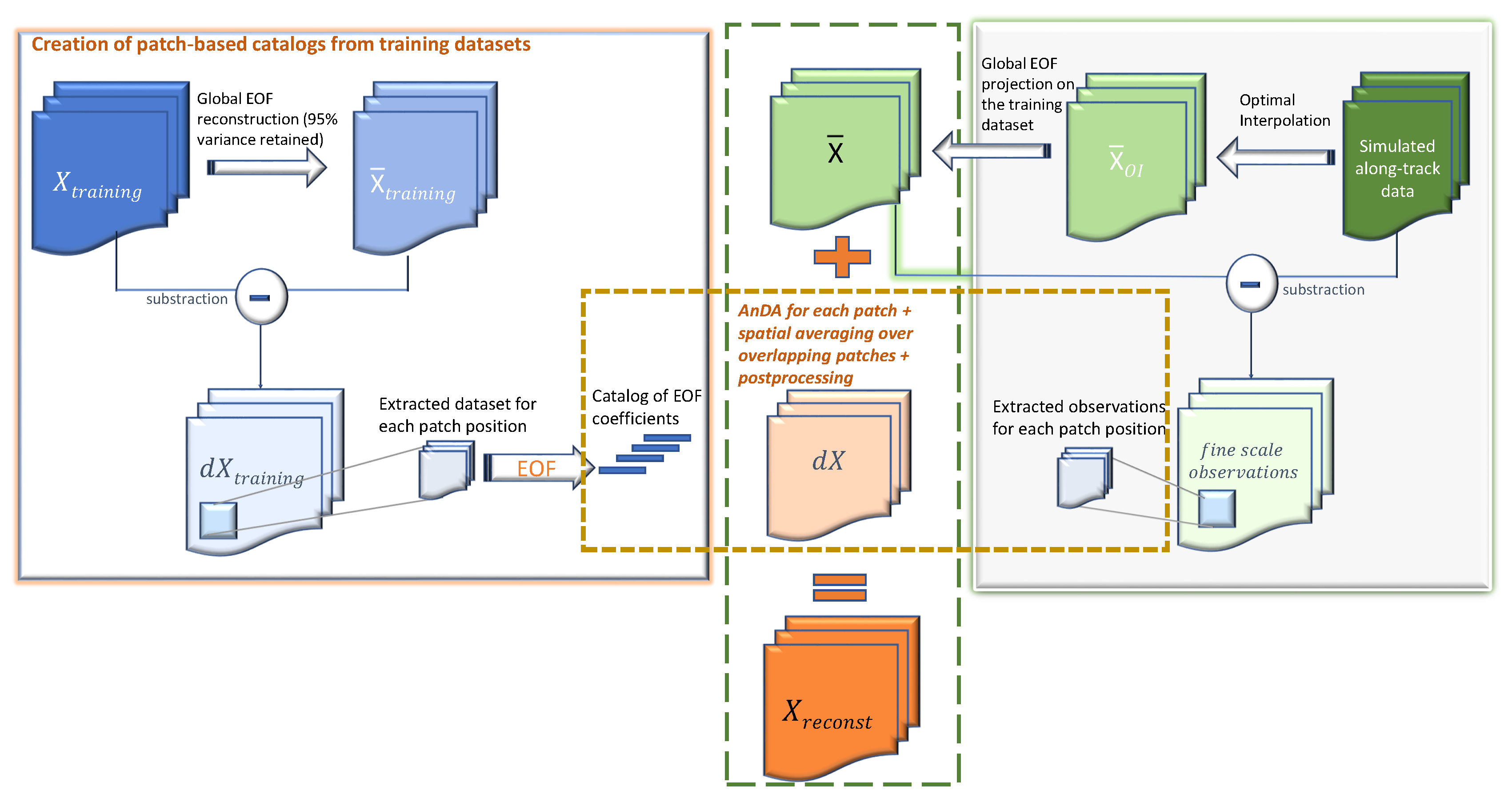
In this work, we build upon our recent advances in analog data assimilation and its application to high-dimensional fields. While the works in [
12,
13] presented the AnDA framework by combining the analog forecasting method and stochastic filtering, these works have only shown applications to geophysical toy models. It was not until the work in [
24] that the AnDA methodology was applied to realistic high dimensional fields, namely, Sea Surface Temperature (SST). Dealing with the curse of dimensionality is a critical challenge, in [
24] we have shown that the use of patch-based representations (a patch is a term used by the image processing community to refer to smaller image parts of a given global image [
25]) combined with EOF-based representations (EOF stands for Empirical Orthogonal Function, a classic dimensionality reduction technique also known as Principal Component Analysis (PCA)) leads to a computationally-efficient interpolation of missing data in SST maps outperforming classical OI-based interpolation schemes. Another development in AnDA applied to high dimensional fields was the introduction of conditional and physically-derived operators [
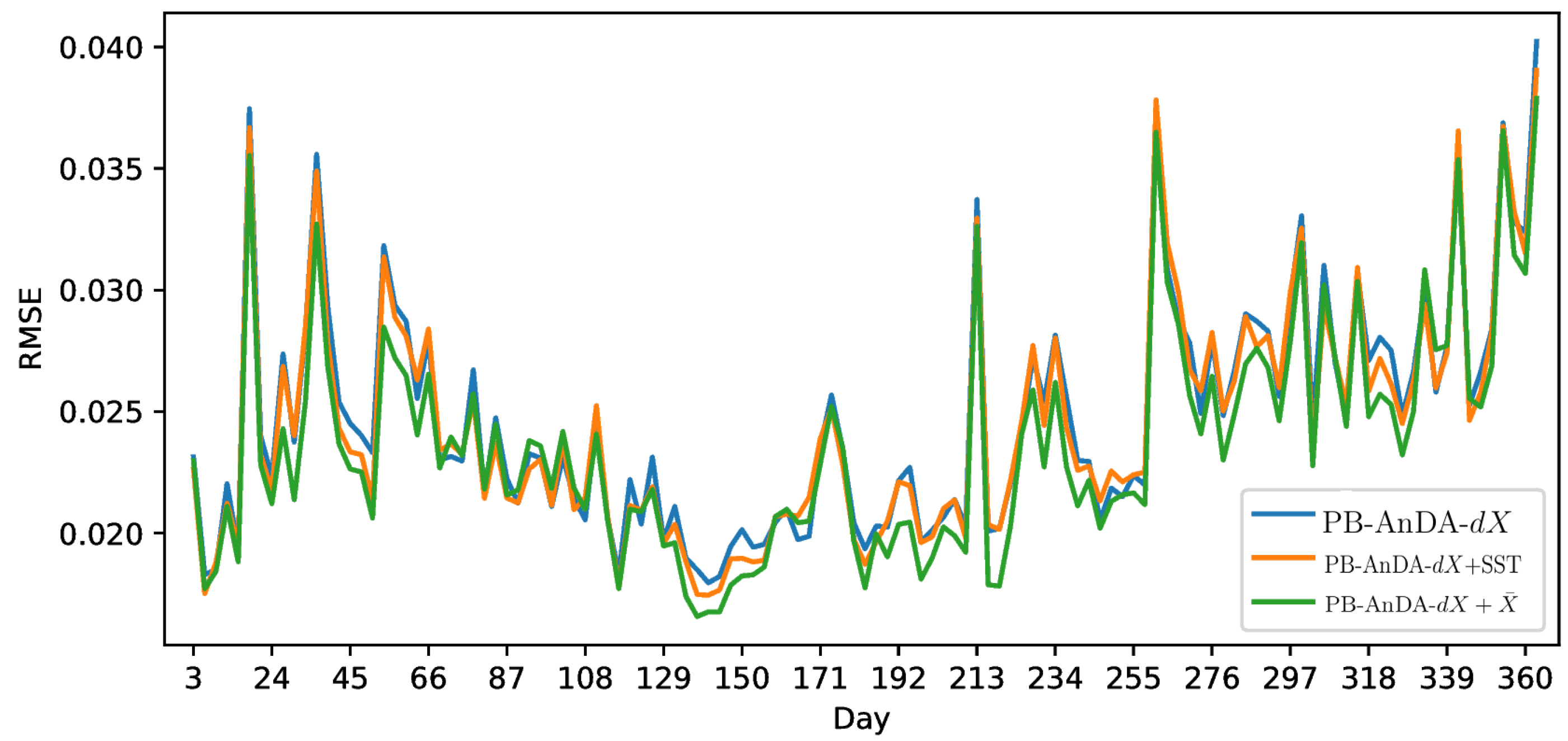
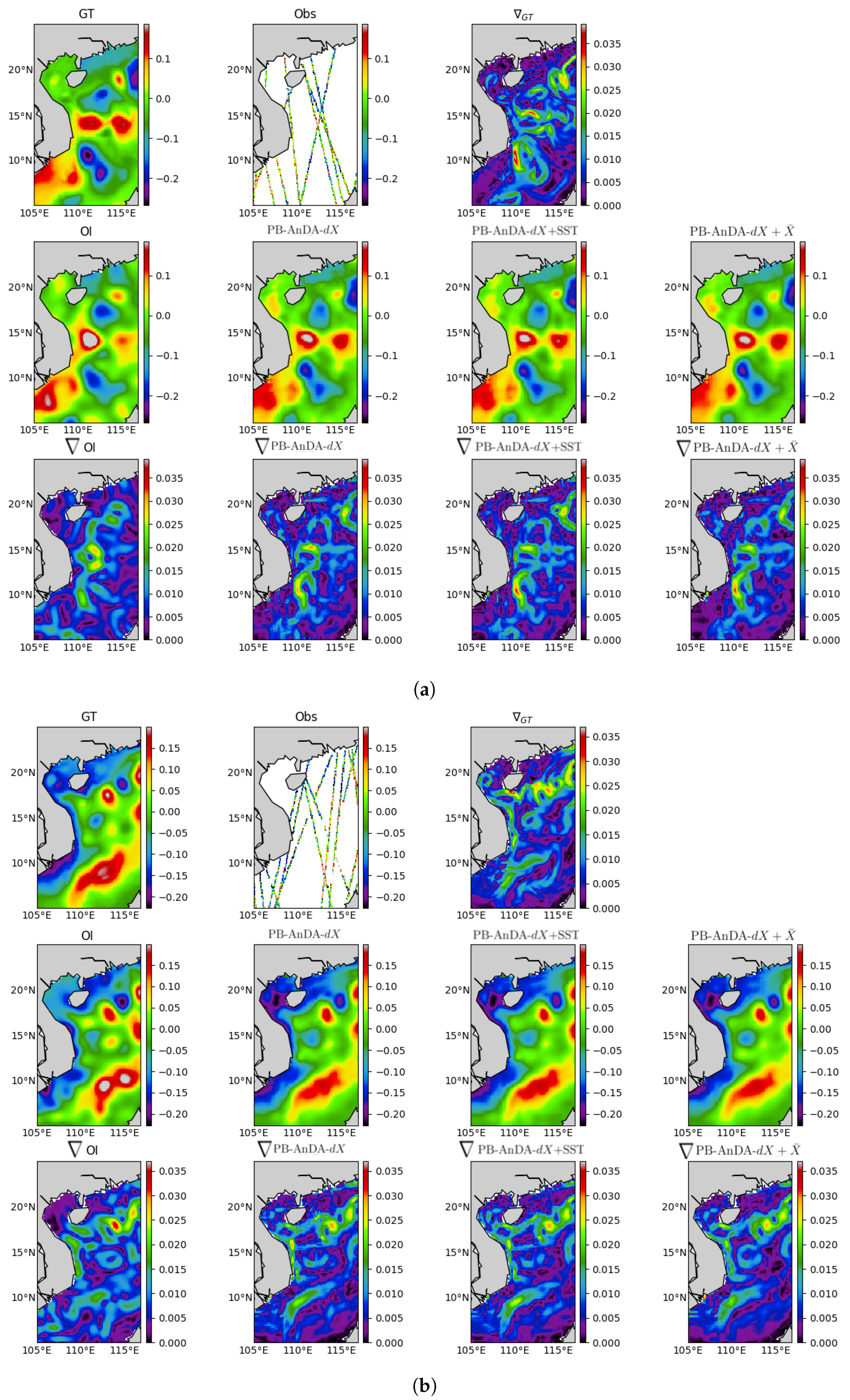
26], where the analog forecasting operators account for the theoretical studies relating to synergies between ocean variables (e.g., SSH and SST) and those highlighting the importance of inter-scale dependencies. In this paper, we make use of these previously developed methodologies and tools and apply the AnDA to Sea Level Anomaly fields. The contribution of this work is two-fold: (i) Confronting AnDA to the reconstruction of an ocean tracer with scarce observations compared to SST (due to the nature of the available altimeters); (ii) designing an Observation System Simulation Experiment (OSSE) based on numerical simulation data to build the archived datasets used for the analog search; (iii) Reconstructing Sea Level Anomaly (SLA) by using SST or large scale SLA as auxiliary variables embedded in the analog regression techniques as shown in
Section 4.
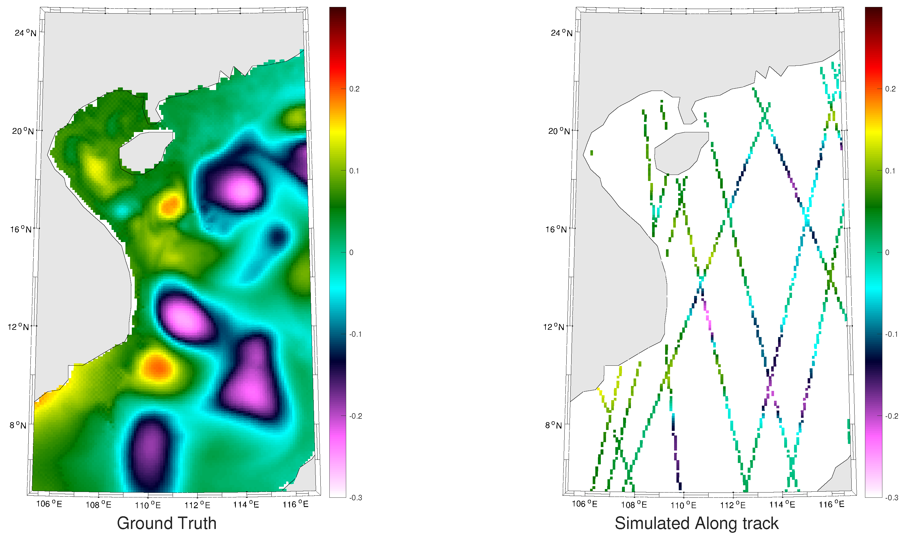
Using OFES (Ocean General Circulation Model (OGCM) for the Earth Simulation) numerical simulations [
27,
28], we design an Observation System Simulation Experiment (OSSE) for a case-study in the South China Sea using real along-track sampling patterns of spaceborne altimeters. Several particular mesoscale variation patterns characterizing this region were studied in the literature, we refer the reader to [
29] and references therein. We also note that our method is not region specific and can be applied to any region of interest . Using the resulting groundtruthed dataset, we perform a qualitative and quantitative evaluation of the proposed scheme, including comparisons to state-of-the-art schemes.
The remainder of the paper is organized as follows:
Section 2 presents the different datasets used in this paper to design an OSSE,
Section 3 gives insights on the classical methods used for mapping SLA from along track data,
Section 4 introduces the proposed analog data assimilation model. Experimental settings are detailed in
Section 5 and results for the considered OSSE are shown in
Section 6.
Section 7 further discusses the key aspects of this work.
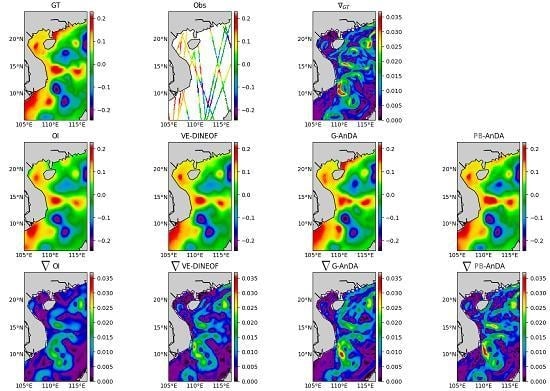
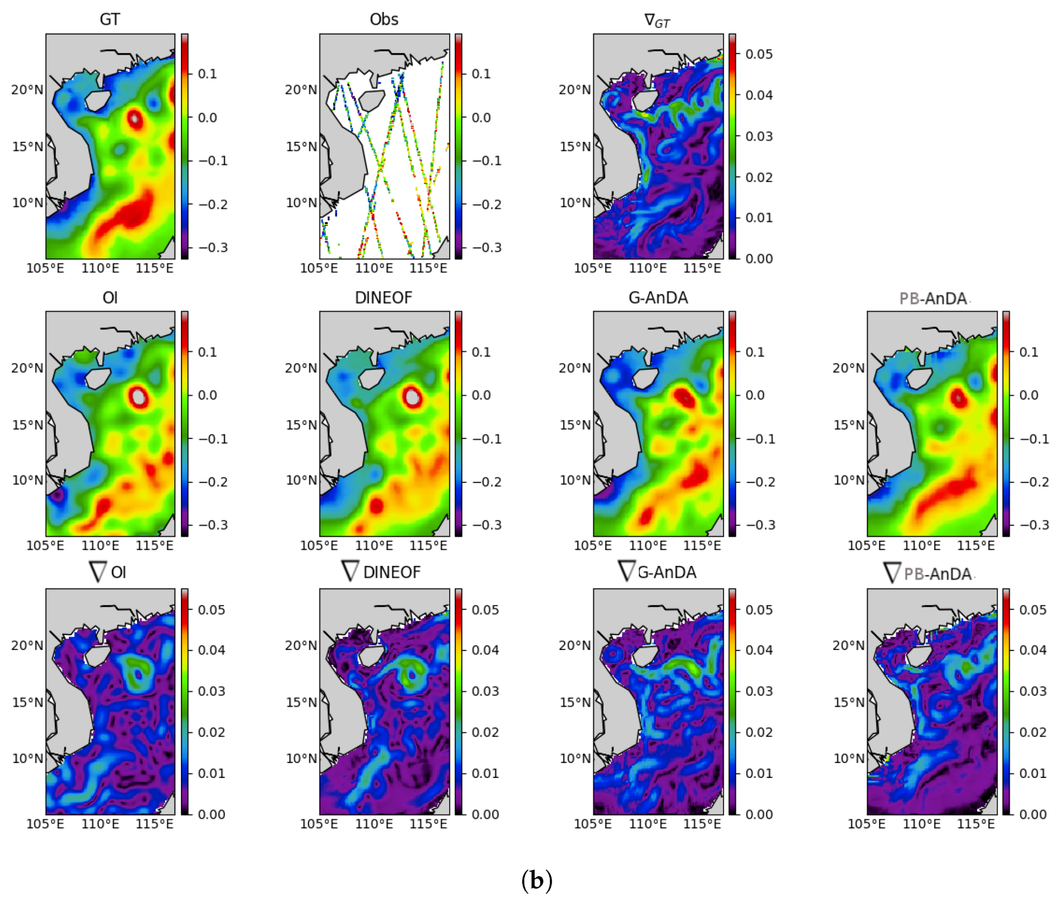
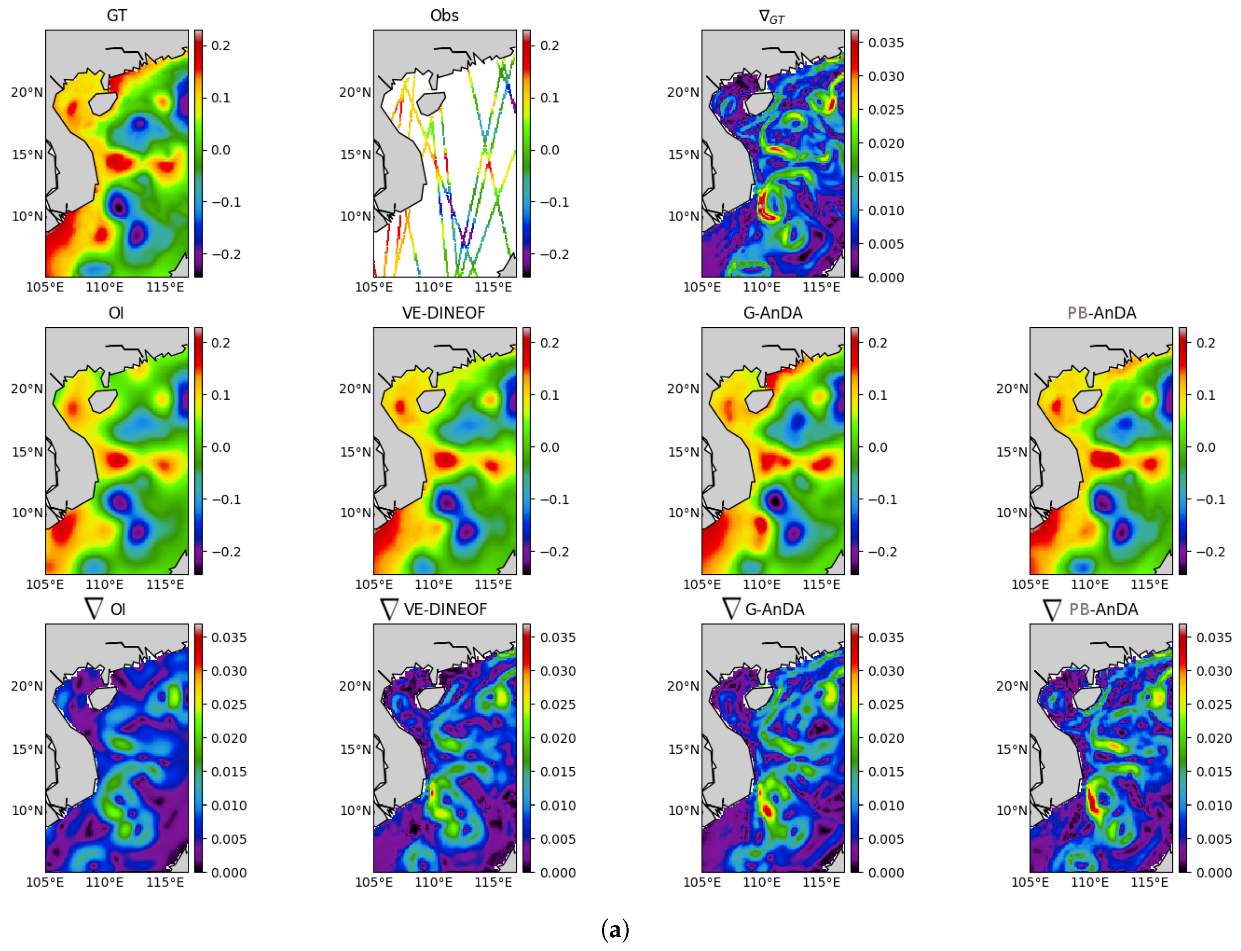
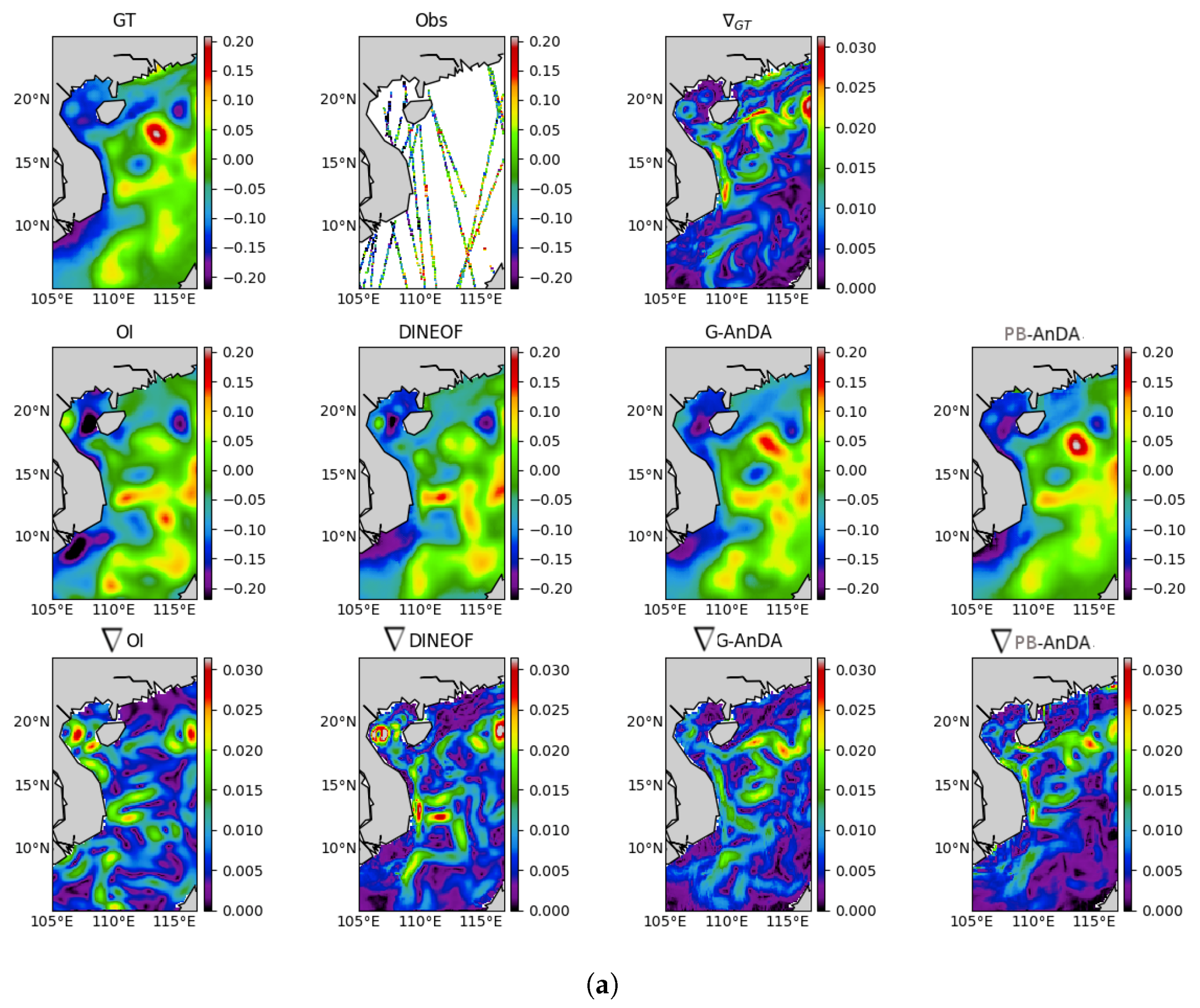
5. Experimental Setting
We detail below the parameter setting of the models evaluated in the reported experiments, including the proposed PB-AnDA scheme:
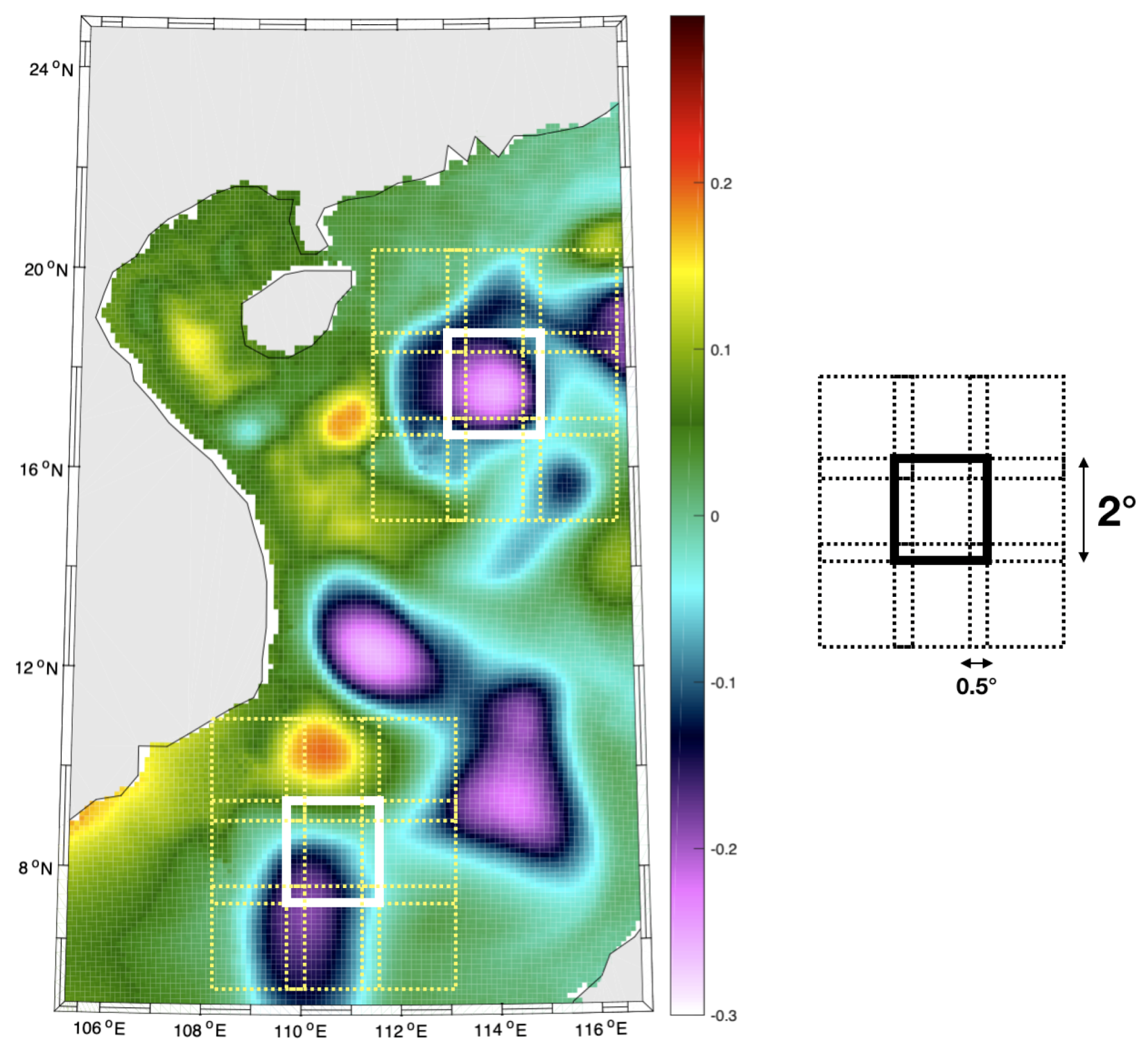
PB-AnDA: We consider patches with 15-dimensional EOF decompositions (), which typically accounts for 99% of the data variance for the considered dataset. The postprocessing step exploits patches and a 15-dimensional EOF decomposition. Regarding the parametrization of the AnEnKS procedure, we experimentally cross-validated the number of nearest neighbors K to 50, the number of ensemble members to 100 and the observation covariance error in Equation (8) is considered to be diagonal and m.
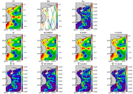
Optimal Interpolation: We apply an Optimal Interpolation to the processed along-track data. It provides the low-resolution component for the proposed PB-AnDA model and a model-driven reference for evaluation purposes. The background field is a null field. We use a Gaussian covariance model with a spatial correlation length of 100 km and a temporal correlation length of 15 days (±5 timesteps since our data is 3-daily). These choices result from a cross-validation experiment.
VE-DINEOF: We apply a second state-of-the-art interpolation scheme using a data-driven strategy solely based on EOF decompositions, namely VE-DINEOF [
36]. Using an iterative reconstruction scheme, VE-DINEOF starts by filling the missing data with a first guess, here along-track pseudo-observation field for along-track data positions and
for missing data positions. For each iteration, the resulting field is projected on the most significant EOF components calculated from the clean catalog data, then missing data positions are updated using pixels from the reconstructed new field. We run this iterative process until convergence. To make this algorithm comparable to the proposed PB-AnDA setting, we perform the reconstruction for each patch position then regroup the results as in PB-AnDA.
G-AnDA: With a view to evaluating the relevance of the patch-based decomposition, we also apply AnDA at the region scale, referred to as G-AnDA. It relies on an EOF-based decomposition of the detail field . We use 150 EOF components, which accounts for more than 99% of the total variance of the SSH dataset. From cross-validation experiments, the associated AnEnKS procedure relies on a locally-linear analog forecasting model with analogs, ensemble members and a diagonal observation covariance similar to as in PB-AnDA.
The patch-based experiments were run on Teralab infrastructure using a multi-core virtual machine (30 CPUs, 64G of RAM). We used the Python toolbox for patch-based analog data assimilation [
24] (available at
github.com/rfablet/PB_ANDA). Optimal Interpolation was implemented on Matlab using [
36]. Throughout the experiments, two metrics are used to assess the performance of the considered interpolation methods: (i) Daily and mean Root Mean Square Error (RMSE) series between the reconstructed SLA fields
X and the groundtruthed ones; (ii) daily and mean correlation coefficient between the fine-scale component
of the reconstructed SLA fields and of the groundtruthed ones. These two metrics allow a good evaluation on image reconstruction capabilities and are widely used in missing data interpolation literature [
38,
39].
7. Discussion
Analog data assimilation can be regarded as a means to fuse ocean models and satellite-derived data. We regard this study as a proof-of-concept, which opens research avenues as well as new directions for operational oceanography. Our results advocate for complementary experiments at the global scale or in different ocean regions for a variety of dynamical situations with a view to further evaluating the relevance of the proposed analog assimilation framework. Such experiments should evaluate the sensitivity of the assimilation with respect to the size of the catalog. The scaling up to the global ocean also suggests investigating computationally-efficient implementation of the analog data assimilation. In this respect, the proposed patch-based framework intrinsically ensures high parallelization performance. From a methodological point of view, a relative weakness of the analog forecasting models (9) may be their low physical interpretation compared with physically-derived priors [
18]. The combination of such physically-derived parameterizations to data-driven strategies appear to be a promising research direction. While we considered an OSSE to evaluate the proposed scheme, future work will investigate applications to real satellite-derived datasets, including the use of independent observation data such as surface drifters’ track data to further assess the performance of the proposed algorithm.
The analog method is at the heart of this work as it is appealing by its implementation ease and its intuitive strategy, but it must not be seen as the only data-driven method adapted to the framework we presented. As long as a data-driven forecasting operator can be derived, other data-driven methods can be investigated [
41,
42]. One promising path is the use of neural networks, as they sparked off a series of breakthroughs in other fields [
42,
43,
44,
45,
46]. While neural network based approaches can lead to better performances due to their superior regressing capabilities, two clear advantages of adopting analog methods are the fact that they do not need a time consuming training phase and that analog methods are easy to understand and interpret compared to black-box approaches such as neural networks.
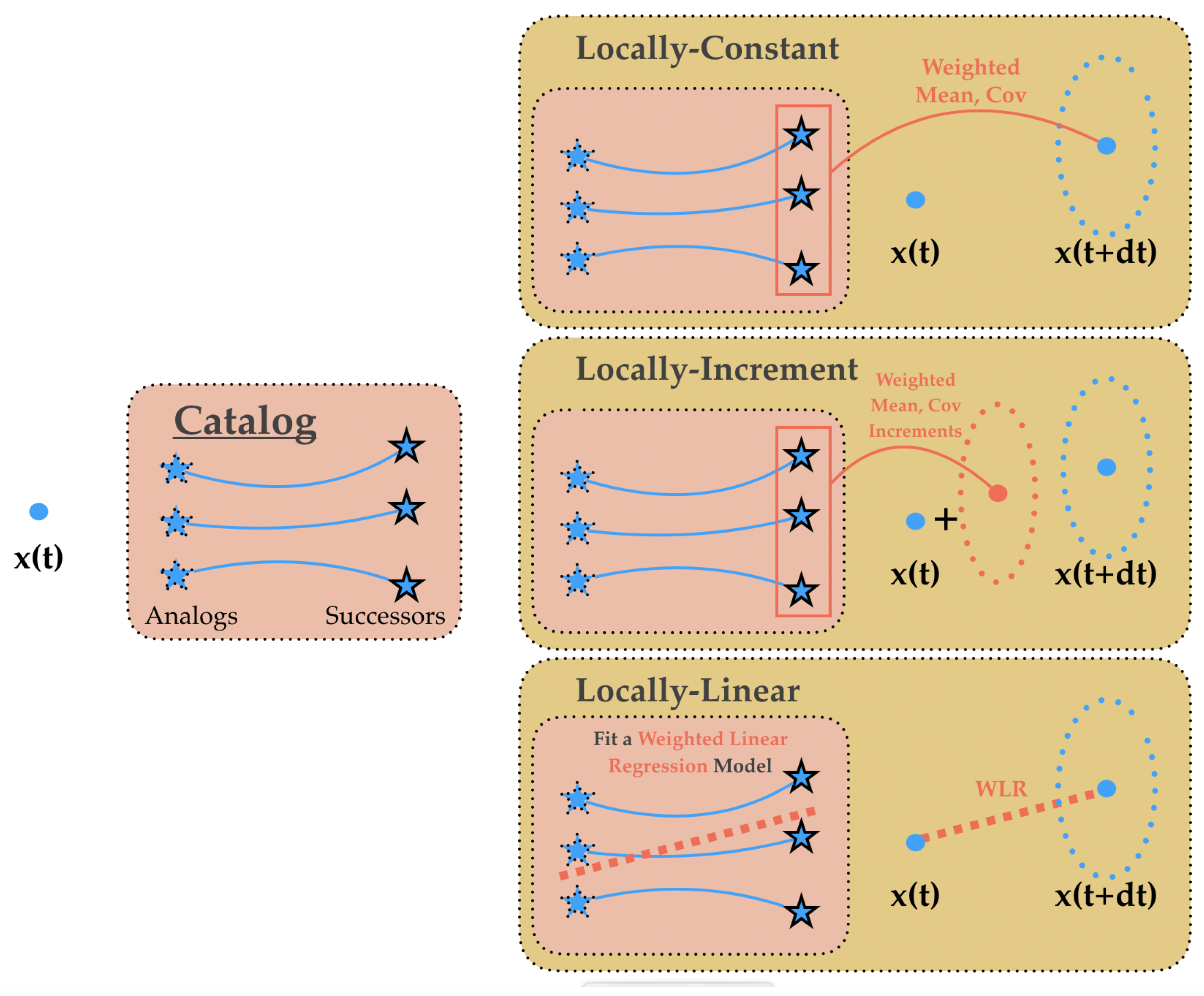
The Analog Data Assimilation method as used in this work relies on several hyperparameters, assumptions and design choices. These considerations are discussed in the following:
In this work, we used all the available data for the creation of the catalog, we expect that a rich dataset is important in increasing the likelihood of finding good analogs, yet a more thorough study is needed to assess the impact of reducing the temporal resolution of the dataset versus reducing the amount of the total available data. To compensate the computational impact of using a large dataset for the search for analogs, we used the FLANN (Fast Library for Approximate Nearest Neighbors) library as in [
26]. This method makes use of tree-indexing techniques and is suitable for this kind of high dimensional applications [
47].
While we used a conditional Gaussian distribution in Equation (9), another alternative is the use of a conditional multinomial distribution. This resorts to sampling one of the analogs’ successors as the forecast. Adopting this alternative would mean that we rely strongly on the archived catalog, so that forecasts of each ensemble member are actual elements of the catalog. This reduces the ability of the model to generate a rich variability of forecast scenes as done by the conditional Gaussian distribution.
While we used a Gaussian kernel in Equation (10), other alternatives include cone kernels [
10] which are more adapted to finding analogs in time series. The performance of our algorithm was slightly improved at the expense of more time execution and an additional hyperparameter to tune empirically, and we decided to prioritize simpler and efficient kernels. Regarding the scale parameter, the median was chosen due to its robustness to outliers.
Although the AnEnKS was used in this work, a possible alternative is the use of an analog based Particle Smoother which drops Gaussian assumptions, however techniques based on particle filters need more ensemble members than their Ensemble Kalman Filter counterparts, thus causing a considerable increase in computational demands which was impractical for our application.
We encourage the reader to refer to the discussion section in [
24] for more insights about the rationale behind the use of patch-based representations and EOF-based dimensionality reduction.
Through the experiments conducted in this work, it was shown that the best performance was always reached using the locally-linear analog operator, which is in line with our previous findings [
13,
24]. An explanation for the superiority of this approach is that it better approximates locally the true dynamical model [
48].
Beyond along-track altimeter data as considered in this study, future missions such as SWOT (NASA/CNES) promise an unprecedented coverage around the globe. More specifically, the large swath is expected to provide a large number of data, urging for the inspection of the potential improvements that this new mission will bring compared to classical along-track data. In the context of analog data assimilation, the interest of SWOT data may be two-fold. First, regarding observation model (8), SWOT mission will both significantly increase the number of available observation data and enable the definition of more complex observation models exploiting for instance velocity-based or vorticity-based criterion. Second, SWOT data might also be used to build representative patch-level catalogs of exemplars. Future work should investigate these two directions using simulated SWOT test-beds [
49].
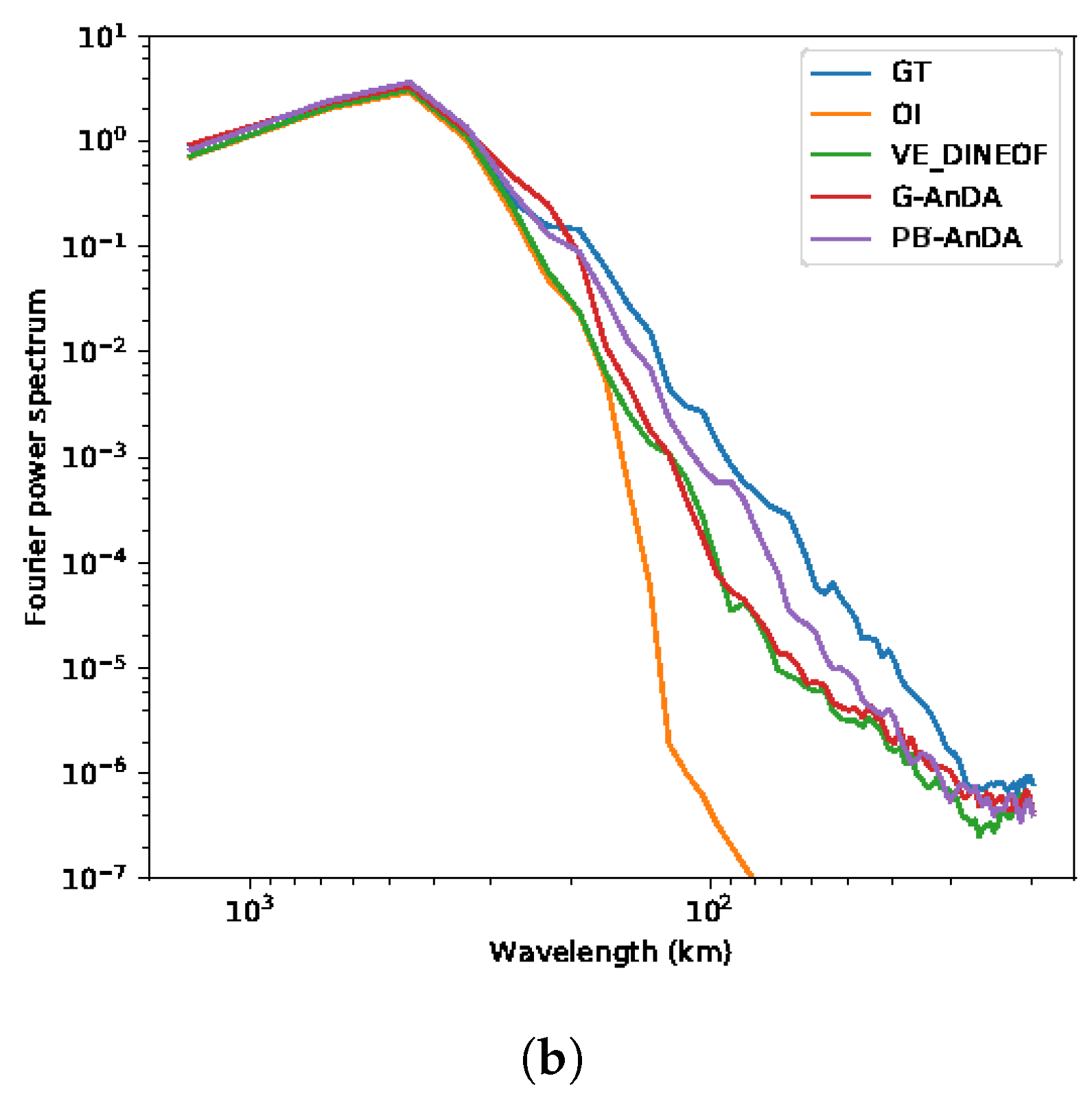
9. Conclusions
This work sheds light on the opportunities that data science methods are offering to improve altimetry in the era of big data. Assuming the availability of high-resolution numerical simulations, we show that Analog Data Assimilation (AnDA) can outperform the Optimal Interpolation method and retrieve smoothed out structures resulting from the sole use of OI both with idealized noise-free and more realistic noisy observations for the considered case study. Importantly, the reported experiments point out the relevance for combining OI for larger scales (above 100 km) whereas the proposed patch-based analog setting successfully applies to the finer-scale range below 100 km. This is in agreement with the recent application of the analog data assimilation to the reconstruction of cloud-free SST fields [
24]. We also demonstrate that AnDA can embed complementary variables in a simple manner through the regression variables used in the locally-linear analog forecasting operator. In agreement with our recent analysis [
17], we demonstrate that the additional use of large-scale SLA information may further improve the reconstruction performance for fine-scale structures.
We may state here the limitations of the present work and possible research avenues for the future. The experiments presented in this work were conducted on a numerical simulation derived dataset. A major future work direction would be then to apply the same procedure on real satellite-derived SLA contaminated with more complex noise models, then investigate the contribution of the use of numerical simulation datasets as catalogs. As combining multi-source datsets can also be challenging when using auxiliary variables relationships with SLA, an interesting experiment for example would be constructing a catalog with real SST observations combined with numerical simulation SLA datasets.
More efforts should be directed to assess the quality of the catalogs (spatio-temporal resolution, total years of measurements to consider, occurence of rare events, etc.). Besides, building a good catalog can represent an opportunity for the use of neural networks based methods, and confronting these powerful regressors to our method is a promising future step. We also note that PB-AnDA can be a relevant candidate for the interpolation of other geophysical variables (e.g., Sea Surface Salinity, Chlorophyll concentrations, etc.) under the condition that they verify the set of assumptions made in this work.

 ,
, 


