Continuous Wavelet Analysis of Leaf Reflectance Improves Classification Accuracy of Mangrove Species

 , ,
, ,
Abstract
1. Introduction
2. Materials and Methods
2.1. Field Sample
2.2. Leaf Reflectance Measurement and Spectra Preprocessing
2.3. Continuous Wavelet Analysis of Leaf Reflectance
2.4. Establishment of Mangrove Species Classification Model
2.4.1. Sample Subset Partition
2.4.2. Feature Extraction
2.4.3. Random Forests Classification
2.5. Evaluation of Classification Model Performance

3. Results
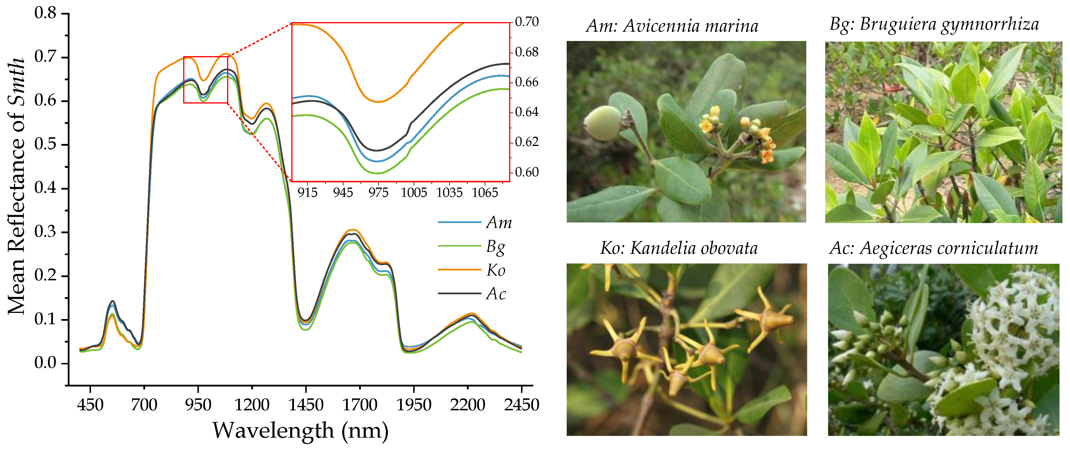
3.1. Mean Reflectance and Wavelet Power Spectra of Mangrove Leaf
3.2. Performance of Classification Models with Reflectance, Derivative and Wavelet Power Spectra
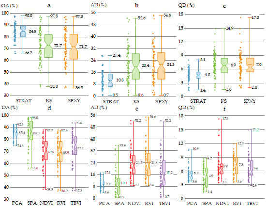
3.3. Performance of Models with Different Sample Subset Partition Methods
3.4. Performance of Classification Models with Different Feature Extraction Methods
4. Discussion
4.1. Continuous Wavelet Analysis for Mangrove Species Classification
4.2. Impact of Sample Subset Partition and Feature Extraction on Classification Accuracy
4.3. Taxonomically Comparing the Accuracy of Mangrove Species Classification
5. Conclusions
- 1)
- Regardless of the effect of sample subset partition and feature extraction methods on the performance of mangrove species classification, CWA with suitable scales has great potential to improve the classification accuracy.
- 2)
- The STRAT method combined with PCA or SPA methods is recommended to improve classification performance.
- 3)
- Compared with the original reflectance spectra, the derivative spectra can significantly improve the classification accuracy.
Supplementary Materials
Author Contributions
Funding
Acknowledgments
Conflicts of Interest
References
- Tam, N.F.Y.; Wong, Y.S. Mangrove soils in removing pollutants from municipal wastewater of different salinities. J. Environ. Qual. 1999, 28, 556–564. [Google Scholar] [CrossRef]
- Murdiyarso, D.; Purbopuspito, J.; Kauffman, J.B.; Warren, M.W.; Sasmito, S.D.; Donato, D.C.; Manuri, S.; Krisnawati, H.; Taberima, S.; Kurnianto, S. The potential of Indonesian mangrove forests for global climate change mitigation. Nat. Clim. Chang. 2015, 5, 1089–1092. [Google Scholar] [CrossRef]
- Mao, L.M.; Zhang, Y.L.; Bi, H. Modern pollen deposits in coastal mangrove swamps from northern Hainan Island, China. J. Coast. Res. 2006, 22, 1423. [Google Scholar] [CrossRef]
- Lugo, A.E.; Snedaker, S.C. The ecology of mangroves. Annu. Rev. Ecol. Syst. 1974, 5, 39–64. [Google Scholar] [CrossRef]
- Jia, M.M.; Liu, M.Y.; Wang, Z.M.; Mao, D.H.; Ren, C.Y.; Cui, H.S. Evaluating the Effectiveness of Conservation on Mangroves: A Remote Sensing-Based Comparison for Two Adjacent Protected Areas in Shenzhen and Hong Kong, China. Remote Sens. 2016, 8, 627. [Google Scholar] [CrossRef]
- Chakravortty, S.; Li, J.; Plaza, A. A Technique for Subpixel Analysis of Dynamic Mangrove Ecosystems with Time-Series Hyperspectral Image Data. IEEE J. Sel. Top. Appl. Earth Obs. Remote Sens. 2018, 11, 1244–1252. [Google Scholar] [CrossRef]
- Richter, R.; Reu, B.; Wirth, C.; Doktor, D.; Vohland, M. The use of airborne hyperspectral data for tree species classification in a species-rich Central European forest area. Int. J. Appl. Earth Obs. Geoinf. 2016, 52, 464–474. [Google Scholar] [CrossRef]
- Wang, D.; Wan, B.; Qiu, P.; Su, Y.; Guo, Q.; Wang, R.; Sun, F.; Wu, X. Evaluating the Performance of Sentinel-2, Landsat 8 and Pléiades-1 in Mapping Mangrove Extent and Species. Remote Sens. 2018, 10, 1468. [Google Scholar] [CrossRef]
- Cao, J.J.; Leng, W.C.; Liu, K.; Liu, L.; He, Z.; Zhu, Y.H. Object-Based Mangrove Species Classification Using Unmanned Aerial Vehicle Hyperspectral Images and Digital Surface Models. Remote Sens. 2018, 10, 89. [Google Scholar] [CrossRef]
- Kuenzer, C.; Bluemel, A.; Gebhardt, S.; Quoc, T.V.; Dech, S. Remote Sensing of Mangrove Ecosystems: A Review. Remote Sens. 2011, 3, 878–928. [Google Scholar] [CrossRef]
- Bullock, E.L.; Fagherazzi, S.; Nardin, W.; Vo-Luong, P.; Nguyen, P.; Woodcock, C.E. Temporal patterns in species zonation in a mangrove forest in the Mekong Delta, Vietnam, using a time series of Landsat imagery. Cont. Shelf Res. 2017, 147, 144–154. [Google Scholar] [CrossRef]
- Heumann, B.W. Satellite remote sensing of mangrove forests: Recent advances and future opportunities. Prog. Phys. Geogr. 2011, 35, 87–108. [Google Scholar] [CrossRef]
- Hauser, L.T.; Vu, G.N.; Nguyen, B.A.; Dade, E.; Nguyen, H.M.; Nguyen, T.T.Q.; Le, T.Q.; Vu, L.H.; Tong, A.T.H.; Pham, H.V. Uncovering the spatio-temporal dynamics of land cover change and fragmentation of mangroves in the Ca Mau peninsula, Vietnam using multi-temporal SPOT satellite imagery (2004–2013). Appl. Geogr. 2017, 86, 197–207. [Google Scholar] [CrossRef]
- Neukermans, G.; Dahdouh-Guebas, F.; Kairo, J.G.; Koedam, N. Mangrove species and stand mapping in GAzi bay (Kenya) using Quickbird satellite imagery. J. Spat. Sci. 2008, 53, 75–86. [Google Scholar] [CrossRef]
- Xin, H.; Liangpei, Z.; Le, W. Evaluation of Morphological Texture Features for Mangrove Forest Mapping and Species Discrimination Using Multispectral IKONOS Imagery. IEEE Geosci. Remote Sens. Lett. 2009, 6, 393–397. [Google Scholar] [CrossRef]
- Heenkenda, M.K.; Joyce, K.E.; Maier, S.W.; Bartolo, R. Mangrove Species Identification: Comparing WorldView-2 with Aerial Photographs. Remote Sens. 2014, 6, 6064–6088. [Google Scholar] [CrossRef]
- Wang, T.; Zhang, H.; Lin, H.; Fang, C. Textural–spectral feature-based species classification of mangroves in Mai Po Nature Reserve from Worldview-3 imagery. Remote Sens. 2015, 8, 24. [Google Scholar] [CrossRef]
- Wang, D.; Wan, B.; Qiu, P.; Su, Y.; Guo, Q.; Wu, X. Artificial Mangrove Species Mapping Using Pléiades-1: An Evaluation of Pixel-Based and Object-Based Classifications with Selected Machine Learning Algorithms. Remote Sens. 2018, 10, 294. [Google Scholar] [CrossRef]
- Govender, M.; Chetty, K.; Naiken, V.; Bulcock, H. A comparison of satellite hyperspectral and multispectral remote sensing imagery for improved classification and mapping of vegetation. Water SA 2008, 34, 147–154. [Google Scholar]
- Wang, L.; Sousa, W.P. Distinguishing mangrove species with laboratory measurements of hyperspectral leaf reflectance. Int. J. Remote Sens. 2009, 30, 1267–1281. [Google Scholar] [CrossRef]
- Prasad, K.A.; Gnanappazham, L. Multiple statistical approaches for the discrimination of mangrove species ofRhizophoraceaeusing transformed field and laboratory hyperspectral data. Geocarto Int. 2015, 31, 891–912. [Google Scholar] [CrossRef]
- Manjunath, K.R.; Kumar, T.; Kundu, N.; Panigrahy, S. Discrimination of mangrove species and mudflat classes using in situ hyperspectral data: A case study of Indian Sundarbans. GISci. Remote Sens. 2013, 50, 400–417. [Google Scholar] [CrossRef]
- Zhang, C.H.; Kovacs, J.M.; Liu, Y.L.; Flores-Verdugo, F.; Flores-de-Santiago, F. Separating Mangrove Species and Conditions Using Laboratory Hyperspectral Data: A Case Study of a Degraded Mangrove Forest of the Mexican Pacific. Remote Sens. 2014, 6, 11673–11688. [Google Scholar] [CrossRef]
- Jia, M.; Zhang, Y.; Wang, Z.; Song, K.; Ren, C. Mapping the distribution of mangrove species in the Core Zone of Mai Po Marshes Nature Reserve, Hong Kong, using hyperspectral data and high-resolution data. Int. J. Appl. Earth Obs. Geoinf. 2014, 33, 226–231. [Google Scholar] [CrossRef]
- Wong, F.K.K.; Fung, T. Combining EO-1 Hyperion and Envisat ASAR data for mangrove species classification in Mai Po Ramsar Site, Hong Kong. Int. J. Remote Sens. 2014, 35, 7828–7856. [Google Scholar] [CrossRef]
- Held, A.; Ticehurst, C.; Lymburner, L.; Williams, N. High resolution mapping of tropical mangrove ecosystems using hyperspectral and radar remote sensing. Int. J. Remote Sens. 2010, 24, 2739–2759. [Google Scholar] [CrossRef]
- Hirano, A.; Madden, M.; Welch, R. Hyperspectral image data for mapping wetland vegetation. Wetlands 2003, 23, 436–448. [Google Scholar] [CrossRef]
- Kamal, M.; Phinn, S. Hyperspectral Data for Mangrove Species Mapping: A Comparison of Pixel-Based and Object-Based Approach. Remote Sens. 2011, 3, 2222–2242. [Google Scholar] [CrossRef]
- Vaglio Laurin, G.; Puletti, N.; Hawthorne, W.; Liesenberg, V.; Corona, P.; Papale, D.; Chen, Q.; Valentini, R. Discrimination of tropical forest types, dominant species, and mapping of functional guilds by hyperspectral and simulated multispectral Sentinel-2 data. Remote Sens. Environ. 2016, 176, 163–176. [Google Scholar] [CrossRef]
- Liu, L.X.; Coops, N.C.; Aven, N.W.; Pang, Y. Mapping urban tree species using integrated airborne hyperspectral and LiDAR remote sensing data. Remote Sens. Environ. 2017, 200, 170–182. [Google Scholar] [CrossRef]
- Sankey, T.; Donager, J.; McVay, J.; Sankey, J.B. UAV lidar and hyperspectral fusion for forest monitoring in the southwestern USA. Remote Sens. Environ. 2017, 195, 30–43. [Google Scholar] [CrossRef]
- Sankey, T.T.; McVay, J.; Swetnam, T.L.; McClaran, M.P.; Heilman, P.; Nichols, M. UAV hyperspectral and lidar data and their fusion for arid and semi-arid land vegetation monitoring. Remote Sens. Ecol. Conserv. 2018, 4, 20–33. [Google Scholar] [CrossRef]
- Melgani, F.; Bruzzone, L. Classification of hyperspectral remote sensing images with support vector machines. IEEE Trans. Geosci. Remote Sens. 2004, 42, 1778–1790. [Google Scholar] [CrossRef]
- Shen, X.; Cao, L. Tree-Species Classification in Subtropical Forests Using Airborne Hyperspectral and LiDAR Data. Remote Sens. 2017, 9, 1180. [Google Scholar] [CrossRef]
- Shen, X.; Cao, L.; Chen, D.; Sun, Y.; Wang, G.B.; Ruan, H.H. Prediction of Forest Structural Parameters Using Airborne Full-Waveform LiDAR and Hyperspectral Data in Subtropical Forests. Remote Sens. 2018, 10, 1729. [Google Scholar] [CrossRef]
- Zhang, N.; Zhang, X.L.; Yang, G.J.; Zhu, C.H.; Huo, L.N.; Feng, H.K. Assessment of defoliation during the Dendrolimus tabulaeformis Tsai et Liu disaster outbreak using UAV-based hyperspectral images. Remote Sens. Environ. 2018, 217, 323–339. [Google Scholar] [CrossRef]
- Chen, W.R.; Yun, Y.H.; Wen, M.; Lu, H.M.; Zhang, Z.M.; Liang, Y.Z. Representative subset selection and outlier detection via isolation forest. Anal. Methods 2016, 8, 7225–7231. [Google Scholar] [CrossRef]
- Lin, Z.D.; Wang, Y.B.; Wang, R.J.; Wang, L.S.; Lu, C.P.; Zhang, Z.Y.; Song, L.T.; Liu, Y. Improvements of the Vis-Nirs Model in the Prediction of Soil Organic Matter Content Using Spectral Pretreatments, Sample Selection, and Wavelength Optimization. J. Appl. Spectrosc. 2017, 84, 529–534. [Google Scholar] [CrossRef]
- Guzmán Q., J.A.; Rivard, B.; Sánchez-Azofeifa, G.A. Discrimination of liana and tree leaves from a Neotropical Dry Forest using visible-near infrared and longwave infrared reflectance spectra. Remote Sens. Environ. 2018, 219, 135–144. [Google Scholar] [CrossRef]
- Li, D.; Wang, X.; Zheng, H.; Zhou, K.; Yao, X.; Tian, Y.; Zhu, Y.; Cao, W.; Cheng, T. Estimation of area- and mass-based leaf nitrogen contents of wheat and rice crops from water-removed spectra using continuous wavelet analysis. Plant Methods 2018, 14, 76. [Google Scholar] [CrossRef]
- Shi, Y.; Huang, W.; González-Moreno, P.; Luke, B.; Dong, Y.; Zheng, Q.; Ma, H.; Liu, L. Wavelet-Based Rust Spectral Feature Set (WRSFs): A Novel Spectral Feature Set Based on Continuous Wavelet Transformation for Tracking Progressive Host–Pathogen Interaction of Yellow Rust on Wheat. Remote Sens. 2018, 10, 525. [Google Scholar] [CrossRef]
- Cheng, T.; Rivard, B.; Sanchez-Azofeifa, A.G.; Feret, J.B.; Jacquemoud, S.; Ustin, S.L. Deriving leaf mass per area (LMA) from foliar reflectance across a variety of plant species using continuous wavelet analysis. ISPRS-J. Photogramm. Remote Sens. 2014, 87, 28–38. [Google Scholar] [CrossRef]
- Cheng, T.; Riano, D.; Ustin, S.L. Detecting diurnal and seasonal variation in canopy water content of nut tree orchards from airborne imaging spectroscopy data using continuous wavelet analysis. Remote Sens. Environ. 2014, 143, 39–53. [Google Scholar] [CrossRef]
- Ali, A.M.; Skidmore, A.K.; Darvishzadeh, R.; van Duren, I.; Holzwarth, S.; Mueller, J. Retrieval of forest leaf functional traits from HySpex imagery using radiative transfer models and continuous wavelet analysis. ISPRS-J. Photogramm. Remote Sens. 2016, 122, 68–80. [Google Scholar] [CrossRef]
- Gross, J.W.; Heumann, B.W. Can flowers provide better spectral discrimination between herbaceous wetland species than leaves? Remote Sens. Lett 2014, 5, 892–901. [Google Scholar] [CrossRef]
- Harrison, D.; Rivard, B.; Sanchez-Azofeifa, A. Classification of tree species based on longwave hyperspectral data from leaves, a case study for a tropical dry forest. Int. J. Appl. Earth Obs. Geoinf. 2018, 66, 93–105. [Google Scholar] [CrossRef]
- Flores-De-Santiago, F.; Kovacs, J.M.; Flores-Verdugo, F. Seasonal changes in leaf chlorophyll a content and morphology in a sub-tropical mangrove forest of the Mexican Pacific. Mar. Ecol.-Prog. Ser. 2012, 444, 57–68. [Google Scholar] [CrossRef]
- Wang, J.J.; Cui, L.J.; Gao, W.X.; Shi, T.Z.; Chen, Y.Y.; Gao, Y. Prediction of low heavy metal concentrations in agricultural soils using visible and near-infrared reflectance spectroscopy. Geoderma 2014, 216, 1–9. [Google Scholar] [CrossRef]
- Holden, H.; LeDrew, E. Spectral Discrimination of Healthy and Non-Healthy Corals Based on Cluster Analysis, Principal Components Analysis, and Derivative Spectroscopy. Remote Sens. Environ. 1998, 65, 217–224. [Google Scholar] [CrossRef]
- Abdel-Rahman, E.M.; Ahmed, F.B.; van den Berg, M. Estimation of sugarcane leaf nitrogen concentration using in situ spectroscopy. Int. J. Appl. Earth Obs. Geoinf. 2010, 12, S52–S57. [Google Scholar] [CrossRef]
- Bruce, L.M.; Morgan, C.; Larsen, S. Automated detection of subpixel hyperspectral targets with continuous and discrete wavelet transforms. IEEE Trans. Geosci. Remote Sens. 2001, 39, 2217–2226. [Google Scholar] [CrossRef]
- Mallat, S.G. A Theory for Multiresolution Signal Decomposition—The Wavelet Representation. IEEE Trans. Pattern Anal. Mach. Intell. 1989, 11, 674–693. [Google Scholar] [CrossRef]
- Blackburn, G.A.; Ferwerda, J.G. Retrieval of chlorophyll concentration from leaf reflectance spectra using wavelet analysis. Remote Sens. Environ. 2008, 112, 1614–1632. [Google Scholar] [CrossRef]
- Cheng, T.; Rivard, B.; Sanchez-Azofeifa, A. Spectroscopic determination of leaf water content using continuous wavelet analysis. Remote Sens. Environ. 2011, 115, 659–670. [Google Scholar] [CrossRef]
- Mallat, S. Zero-Crossings of a Wavelet Transform. IEEE Trans. Inf. Theory 1991, 37, 1019–1033. [Google Scholar] [CrossRef]
- Bruce, L.M.; Li, J. Wavelets for computationally efficient hyperspectral derivative analysis. IEEE Trans. Geosci. Remote Sens. 2001, 39, 1540–1546. [Google Scholar] [CrossRef]
- Miller, J.R.; Hare, E.W.; Wu, J. Quantitative Characterization of the Vegetation Red Edge Reflectance. 1. An Inverted-Gaussian Reflectance Model. Int. J. Remote Sens. 1990, 11, 1755–1773. [Google Scholar] [CrossRef]
- Torrence, C.; Compo, G.P. A practical guide to wavelet analysis. Bull Amer Meteorol Soc 1998, 79, 61–78. [Google Scholar] [CrossRef]
- Rivard, B.; Feng, J.; Gallie, A.; Sanchez-Azofeifa, A. Continuous wavelets for the improved use of spectral libraries and hyperspectral data. Remote Sens. Environ. 2008, 112, 2850–2862. [Google Scholar] [CrossRef]
- Du, P.; Kibbe, W.A.; Lin, S.M. Improved peak detection in mass spectrum by incorporating continuous wavelet transform-based pattern matching. Bioinformatics 2006, 22, 2059–2065. [Google Scholar] [CrossRef]
- Cheng, T.; Rivard, B.; Sanchez-Azofeifa, G.A.; Feng, J.; Calvo-Polanco, M. Continuous wavelet analysis for the detection of green attack damage due to mountain pine beetle infestation. Remote Sens. Environ. 2010, 114, 899–910. [Google Scholar] [CrossRef]
- Roth, K.L.; Dennison, P.E.; Roberts, D.A. Comparing endmember selection techniques for accurate mapping of plant species and land cover using imaging spectrometer data. Remote Sens. Environ. 2012, 127, 139–152. [Google Scholar] [CrossRef]
- Lyons, M.B.; Keith, D.A.; Phinn, S.R.; Mason, T.J.; Elith, J. A comparison of resampling methods for remote sensing classification and accuracy assessment. Remote Sens. Environ. 2018, 208, 145–153. [Google Scholar] [CrossRef]
- Kennard, R.W.; Stone, L.A. Computer Aided Design of Experiments. Technometrics 1969, 11, 137. [Google Scholar] [CrossRef]
- Galvao, R.K.; Araujo, M.C.; Jose, G.E.; Pontes, M.J.; Silva, E.C.; Saldanha, T.C. A method for calibration and validation subset partitioning. Talanta 2005, 67, 736–740. [Google Scholar] [CrossRef] [PubMed]
- Prospere, K.; McLaren, K.; Wilson, B. Plant Species Discrimination in a Tropical Wetland Using In Situ Hyperspectral Data. Remote Sens. 2014, 6, 8494–8523. [Google Scholar] [CrossRef]
- Cliff, N. The Eigenvalues-Greater-Than-One Rule and the Reliability of Components. Psychol. Bull. 1988, 103, 276–279. [Google Scholar] [CrossRef]
- Araujo, M.C.U.; Saldanha, T.C.B.; Galvao, R.K.H.; Yoneyama, T.; Chame, H.C.; Visani, V. The successive projections algorithm for variable selection in spectroscopic multicomponent analysis. Chemom. Intell. Lab. Syst. 2001, 57, 65–73. [Google Scholar] [CrossRef]
- Thenkabail, P.S.; Smith, R.B.; Pauw, E.D. Hyperspectral Vegetation Indices and Their Relationships with Agricultural Crop Characteristics. Remote Sens. Environ. 2000, 71, 158–182. [Google Scholar] [CrossRef]
- Rouse, J.W., Jr.; Haas, R.H.; Schell, J.A.; Deering, D.W. Monitoring the Vernal Advancement and Retrogradation (Green Wave Effect) of Natural Vegetation; Texas A&M University: College Station, TX, USA, 1973; pp. 1–137. [Google Scholar]
- Pearson, R.L.; Miller, L.D. Remote mapping of standing crop biomass for estimation of the productivity of the shortgrass prairie. Proc. Remote Sens. Environ. 1972, 8, 1355. [Google Scholar]
- Pacheco-Labrador, J.; Gonzalez-Cascon, R.; Martin, M.P.; Riano, D. Understanding the optical responses of leaf nitrogen in Mediterranean Holm oak (Quercus ilex) using field spectroscopy. Int. J. Appl. Earth Obs. Geoinf. 2014, 26, 105–118. [Google Scholar] [CrossRef]
- Breiman, L.I.; Friedman, J.H.; Olshen, R.A.; Stone, C.J. Classification and Regression Trees (CART). Encycl. Ecol. 1984, 40, 582–588. [Google Scholar]
- Ismail, R.; Mutanga, O.; Kumar, L. Modeling the Potential Distribution of Pine Forests Susceptible to Sirex Noctilio Infestations in Mpumalanga, South Africa. Trans. Gis 2010, 14, 709–726. [Google Scholar] [CrossRef]
- Breiman, L. Random forests. Mach. Learn. 2001, 45, 5–32. [Google Scholar] [CrossRef]
- Grossmann, E.; Ohmann, J.; Kagan, J.; May, H.; Gregory, M. Mapping ecological systems with a random foret model: Tradeoffs between errors and bias. Gap Anal. Bull. 2010, 17, 16–22. [Google Scholar]
- Lawrence, R.L.; Wood, S.D.; Sheley, R.L. Mapping invasive plants using hyperspectral imagery and Breiman Cutler classifications (RandomForest). Remote Sens. Environ. 2006, 100, 356–362. [Google Scholar] [CrossRef]
- Dahinden, C. An improved Random Forests approach with application to the performance prediction challenge datasets. Hands Pattern Recognit. 2011, 1, 223–230. [Google Scholar]
- Nishii, R.; Tanaka, S. Accuracy and inaccuracy assessments in land-cover classification. IEEE Trans. Geosci. Remote Sens. 1999, 37, 491–498. [Google Scholar] [CrossRef]
- Pontius, R.G., Jr.; Millones, M. Death to Kappa: Birth of quantity disagreement and allocation disagreement for accuracy assessment. Int. J. Remote Sens. 2011, 32, 4407–4429. [Google Scholar]
- Nurmemet, I.; Ghulam, A.; Tiyip, T.; Elkadiri, R.; Ding, J.L.; Maimaitiyiming, M.; Abliz, A.; Sawut, M.; Zhang, F.; Abliz, A.; et al. Monitoring Soil Salinization in Keriya River Basin, Northwestern China Using Passive Reflective and Active Microwave Remote Sensing Data. Remote Sens. 2015, 7, 8803–8829. [Google Scholar] [CrossRef]
- Li, D.; Cheng, T.; Zhou, K.; Zheng, H.B.; Yao, X.; Tian, Y.C.; Zhu, Y.; Cao, W.X. WREP: A wavelet-based technique for extracting the red edge position from reflectance spectra for estimating leaf and canopy chlorophyll contents of cereal crops. ISPRS-J. Photogramm. Remote Sens. 2017, 129, 103–117. [Google Scholar] [CrossRef]
- Zhan, X.Y.; Zhao, N.; Lin, Z.Z.; Wu, Z.S.; Yuan, R.J.; Qiao, Y.J. Effect of Algorithms for Calibration Set Selection on Quantitatively Determining Asiaticoside Content in Centella Total Glucosides by Near Infrared Spectroscopy. Spectrosc. Spectr. Anal. 2014, 34, 3267–3272. [Google Scholar] [CrossRef]
- Thenkabail, P.S.; Lyon, J.G. Hyperspectral Remote Sensing of Vegetation; CRC Press: Boca Raton, FL, USA, 2016. [Google Scholar]
- Thenkabail, P.S.; Enclona, E.A.; Ashton, M.S.; Van Der Meer, B. Accuracy assessments of hyperspectral waveband performance for vegetation analysis applications. Remote Sens. Environ. 2004, 91, 354–376. [Google Scholar] [CrossRef]
- Curran, P.J. Remote-Sensing of Foliar Chemistry. Remote Sens. Environ. 1989, 30, 271–278. [Google Scholar] [CrossRef]
- Asner, G.P.; Martin, R.E. Canopy phylogenetic, chemical and spectral assembly in a lowland Amazonian forest. New Phytol. 2011, 189, 999–1012. [Google Scholar] [CrossRef]
- Kiang, N.Y.; Siefert, J.; Govindjee; Blankenship, R.E. Spectral signatures of photosynthesis. I. Review of Earth organisms. Astrobiology 2007, 7, 222–251. [Google Scholar] [CrossRef]
- Piiroinen, R.; Heiskanen, J.; Mottus, M.; Pellikka, P. Classification of crops across heterogeneous agricultural landscape in Kenya using AisaEAGLE imaging spectroscopy data. Int. J. Appl. Earth Obs. Geoinf. 2015, 39, 1–8. [Google Scholar] [CrossRef]


| Time | Sampling Location | Sample Size | Species |
|---|---|---|---|
| 2017.01 | Futian national mangrove nature reserve, Shenzhen | 47 | Am; Bg; Ko |
| 2017.04 | Shankou national mangrove nature reserve, Beihai | 19 | Ac; Bg; Ko |
| Dangjiang Town, Beihai | 22 | Ac; Ko | |
| Gaoqiao mangrove nature reserve, Zhanjiang | 56 | Ac; Bg; Ko | |
| Shatian Town, Beihai | 23 | Ac; Am | |
| Beihai coastal national wetland park, Beihai | 24 | Am; Ko | |
| 2017.10 | Futian national mangrove nature reserve, Shenzhen | 51 | Am; Ko |
| 2018.05 | Gaoqiao mangrove nature reserve, Zhanjiang | 59 | Ac; Bg; Ko |
| Spectra | Smth | Smth_1 | Smth_2 | Smth_4 | Smth_8 | Smth_16 | Smth_32 | Smth_64 | Smth_128 |
|---|---|---|---|---|---|---|---|---|---|
| Num_Comps | 5 | 5 | 7 | 7 | 6 | 6 | 6 | 5 | 5 |
| Explained (%) | 99.16 | 93.55 | 92.73 | 95.52 | 96.14 | 97.30 | 97.58 | 96.76 | 98.59 |
| Spectra | Der | Der_1 | Der_2 | Der_4 | Der_8 | Der_16 | Der_32 | Der_64 | Der_128 |
| Num_Comps | 6 | 13 | 12 | 9 | 6 | 4 | 5 | 5 | 5 |
| Explained (%) | 96.01 | 84.90 | 84.65 | 91.79 | 96.12 | 96.40 | 97.57 | 97.73 | 98.56 |
| Spectra | Number of Models | OA (%) | AD (%) | QD (%) | |||||||||
|---|---|---|---|---|---|---|---|---|---|---|---|---|---|
| Max | Min | Mean | SD | Max | Min | Mean | SD | Max | Min | Mean | SD | ||
| Smth | 15 | 86.3 | 52.8 | 68.5 | 11.6 | 39.3 | 8.4 | 24.4 | 10.8 | 8.8 | 5.4 | 7.2 | 1.0 |
| Smth_1 | 15 | 88.0 | 56.9 | 69.9 | 10.6 | 36.0 | 6.5 | 22.7 | 9.2 | 11.0 | 5.4 | 7.4 | 1.9 |
| Smth_2 | 15 | 91.1 | 65.2 | 77.7 | 9.3 | 28.3 | 4.3 | 16.0 | 7.9 | 9.9 | 4.6 | 6.3 | 1.8 |
| Smth_4 | 15 | 97.1 | 76.3 | 87.0 | 7.0 | 17.4 | 0.8 | 8.4 | 5.1 | 10.8 | 2.1 | 4.6 | 2.4 |
| Smth_8 | 15 | 97.6 | 72.5 | 84.7 | 8.6 | 20.5 | 0.9 | 10.5 | 6.8 | 8.7 | 1.6 | 4.7 | 1.9 |
| Smth_16 | 15 | 92.3 | 71.0 | 82.5 | 7.6 | 23.4 | 3.6 | 12.5 | 6.4 | 7.8 | 3.5 | 5.1 | 1.4 |
| Smth_32 | 15 | 89.9 | 61.8 | 76.4 | 10.1 | 31.2 | 5.3 | 17.7 | 9.3 | 8.7 | 4.6 | 5.9 | 1.1 |
| Smth_64 | 15 | 89.8 | 57.3 | 74.7 | 11.1 | 29.5 | 5.4 | 17.5 | 8.3 | 17.3 | 4.8 | 7.8 | 3.6 |
| Smth_128 | 15 | 86.5 | 48.7 | 67.0 | 13.2 | 42.4 | 8.7 | 24.7 | 10.9 | 14.9 | 4.9 | 8.3 | 3.0 |
| Der | 15 | 93.0 | 69.6 | 81.9 | 8.9 | 24.2 | 3.7 | 13.0 | 7.4 | 8.9 | 3.0 | 5.0 | 1.7 |
| Der_1 | 15 | 84.1 | 36.9 | 57.3 | 17.0 | 54.6 | 7.8 | 34.3 | 16.6 | 10.8 | 5.5 | 8.4 | 1.6 |
| Der_2 | 15 | 88.7 | 55.0 | 70.0 | 11.4 | 37.6 | 4.7 | 22.7 | 10.7 | 9.8 | 4.4 | 7.3 | 1.5 |
| Der_4 | 15 | 97.3 | 61.1 | 79.9 | 12.6 | 30.5 | 1.0 | 15.2 | 10.7 | 9.0 | 1.8 | 5.0 | 2.1 |
| Der_8 | 15 | 98.0 | 70.7 | 85.6 | 8.5 | 21.2 | 0.5 | 10.1 | 6.8 | 8.2 | 1.4 | 4.4 | 1.8 |
| Der_16 | 15 | 96.8 | 67.2 | 82.2 | 9.6 | 25.8 | 1.2 | 12.9 | 7.9 | 8.1 | 2.0 | 5.0 | 1.8 |
| Der_32 | 15 | 91.2 | 61.8 | 80.7 | 8.8 | 28.0 | 4.4 | 13.4 | 7.1 | 10.2 | 4.0 | 5.9 | 2.1 |
| Der_64 | 15 | 88.3 | 66.0 | 75.5 | 7.8 | 26.9 | 6.6 | 18.2 | 7.1 | 9.0 | 4.9 | 6.3 | 1.0 |
| Der_128 | 15 | 86.5 | 54.5 | 71.6 | 11.5 | 36.1 | 7.6 | 20.5 | 9.4 | 13.8 | 5.2 | 7.8 | 2.5 |
| Sum | 270 | ||||||||||||
| Wavebands Selected by SPA | Wavebands Selected by VIs | |
|---|---|---|
| Wavelength (nm) | 405; 685; 690; 695; 700; 705; 710; 715; 720; 725; 730; 735; 745; 800; 1145; 1650; 1655; 1730; 1875; 1885; 1890; 2245; 2320; 2450 | 405; 515; 605; 685; 690; 695; 700; 715; 730; 745; 765; 800; 855; 1385; 1390; 1620; 1650; 1655; 1695; 1730; 1740; 1870; 1945; 1970; 2185; 2235; 2245; 2250; 2255; 2260; 2320; 2450 |
© 2019 by the authors. Licensee MDPI, Basel, Switzerland. This article is an open access article distributed under the terms and conditions of the Creative Commons Attribution (CC BY) license (http://creativecommons.org/licenses/by/4.0/).
Share and Cite
Xu, Y.; Wang, J.; Xia, A.; Zhang, K.; Dong, X.; Wu, K.; Wu, G. Continuous Wavelet Analysis of Leaf Reflectance Improves Classification Accuracy of Mangrove Species. Remote Sens. 2019, 11, 254. https://doi.org/10.3390/rs11030254
Xu Y, Wang J, Xia A, Zhang K, Dong X, Wu K, Wu G. Continuous Wavelet Analysis of Leaf Reflectance Improves Classification Accuracy of Mangrove Species. Remote Sensing. 2019; 11(3):254. https://doi.org/10.3390/rs11030254
Chicago/Turabian StyleXu, Yi, Junjie Wang, Anquan Xia, Kangyong Zhang, Xuanyan Dong, Kaipeng Wu, and Guofeng Wu. 2019. "Continuous Wavelet Analysis of Leaf Reflectance Improves Classification Accuracy of Mangrove Species" Remote Sensing 11, no. 3: 254. https://doi.org/10.3390/rs11030254
APA StyleXu, Y., Wang, J., Xia, A., Zhang, K., Dong, X., Wu, K., & Wu, G. (2019). Continuous Wavelet Analysis of Leaf Reflectance Improves Classification Accuracy of Mangrove Species. Remote Sensing, 11(3), 254. https://doi.org/10.3390/rs11030254