Assessment of Level-3 Gridded Global Precipitation Mission (GPM) Products Over Oceans

Abstract

The performance of Level-3 gridded Global Precipitation Mission (GPM)-based precipitation products (IMERG, Integrated Multi-satellite Retrievals for GPM) is assessed against two references over oceans: the OceanRAIN dataset, derived from oceanic shipboard disdrometers, and a satellite-based radar product (the Level-3 Dual-frequency Precipitation Radar, 3DPRD). Daily IMERG products (early, late, final) and microwave-only (MW) and Infrared-only (IR) precipitation components are evaluated at four different spatial resolutions (0.5°, 1°, 2°, and 3°) during a 3-year study period (March 2014–February 2017). Their performance is assessed based on both categorical and continuous performance metrics, including correlation coefficient, probability of detection, success ratio, bias, and root mean square error (RMSE). A triple collocation analysis (TCA) is also presented to further investigate the performance of these satellite-based products. Overall, the IMERG products show an underestimation with respect to OceanRAIN. Rain events in OceanRAIN are correctly detected by all IMERG products ~80% of the times. IR estimates show relatively large errors and low correlations with OceanRAIN compared to the other products. On the other hand, the MW component performs better than other products in terms of both categorical and continuous statistics. TCA reveals that 3DPRD performs consistently better than OceanRAIN in terms of RMSE and coefficient of determination at all spatial resolutions. This work is part of a larger effort to validate GPM products over nontraditional regions such as oceans.

1. Introduction

Global precipitation data play a key role across numerous applications such as hazard mitigation, terrestrial hydrology, climate change studies, as well as agriculture and irrigation practices [1,2,3,4]. The National Aeronautics and Space Administration (NASA) and the Japan Aerospace Exploration Agency (JAXA) launched the Global Precipitation Measurement (GPM) mission in 2014, which carries an advanced radar (Dual-frequency Precipitation Radar; DPR) and a radiometer system (GPM Microwave Imager, GMI) to measure global precipitation from space [5]. Certain geographical locations, such as oceans and impervious terrain regions, entirely depend on satellite measurements as the only source of precipitation information [6] and the Integrated Multi-satellite Retrievals for GPM (IMERG) products represent the state-of-the-art product for global precipitation estimation. The IMERG algorithm fuses information from several satellite-based microwave and infrared precipitation estimates, as well as ground gauge information.

The measurement and validation of oceanic precipitation are vital for understanding the global water cycle, as most of the global precipitation occurs over oceans [7]. Due to the scarcity of surface measurements over oceans, satellite-based precipitation observations often represent the only source of information. It is critical to characterize errors associated with these products, as these errors may lead to erroneous conclusions in many applications, e.g., fresh water budgets, currents, cyclones and hurricanes propagation, and El Niño-Southern Oscillation (ENSO) cycle predictions. The GPM Ground Validation (GV) group utilizes reference data obtained from multiple sources, including radar networks and ground-based measurements to validate satellite precipitation measurements [8]. However, validating satellite products over oceans is more challenging because of their inaccessibility and geographical extent (~75% of earth’s surface). Past efforts have used weather radars situated on islands and coastlines [9]. Over the years, rain gauge measurements onboard cruise, merchant, and research ships have been used to estimate oceanic precipitation in addition to tropical buoy gauge arrays and manual observations from voluntary observation ships [10,11,12]. Rain gauges mounted on buoys take point measurements with high temporal resolution, but are easily influenced by wind speed, which can lead to erroneous estimates. In contrast, satellite precipitation estimates have relatively high spatial coverage but lower temporal resolution [13].

Thanks to the launch of the Tropical Rainfall Measurement Mission (TRMM) in 1997 and GPM in 2014, satellite precipitation products have provided useful information on oceanic precipitation quantification and patterns. Bowman [14] and Serra and McPhaden [15,16] compared TRMM-based precipitation retrievals against rain gauge data from ocean buoys in the Pacific and Atlantic Oceans. These studies highlighted the uncertainties associated with an area-averaged and a point measurement-based comparison. In order to fill this gap, scientific groups, such as the International Precipitation Working Group (IPWG) and the GPM GV group, have pressed the need for improved and robust oceanic precipitation surface measurements and associated errors [17]. OceanRAIN (Ocean Rainfall and Ice-phase precipitation measurement Network) is an effort to provide high quality along-track shipboard precipitation data for surface validation over global oceans [18]. IMERG V03 has been evaluated against OceanRAIN precipitation and showed an underestimation of shallow tropical rainfall [19]. Another recent study used OceanRAIN precipitation data for evaluating the HOAPS (Hamburg Ocean Atmosphere Parameters and fluxes from Satellite data) precipitation product across the Atlantic Ocean [20]. This study highlighted that the differences between HOAPS and OceanRAIN are governed by the point-to-area (along track-pixel) effect rather than the precipitation regime itself. Although some efforts have been done in this direction, there is still a need for more evaluation of satellite-based products (particularly their most recent versions) over oceans.

The overall objective of this study is to investigate and better understand how the latest Version 05 of the IMERG products and components performs across oceans at different spatial resolutions. As there is no reference that is continuously available both in time and space over oceans, IMERG products are evaluated against the OceanRAIN precipitation dataset and the Level-3 DPR product, 3DPRD. This work assesses all products at the daily temporal resolution and at four different spatial resolutions, i.e., 0.5°, 1°, 2° and 3°. The GPM GV group lays special emphasis on validation studies in “nontraditional” regions like oceans and this study fits well within this wider effort. The datasets and methodology used in this study are presented in Section 2. Results are described in Section 3 and discussed in Section 4, whereas Section 5 summarizes the main conclusions and presents future research directions.

2. Materials and Methods

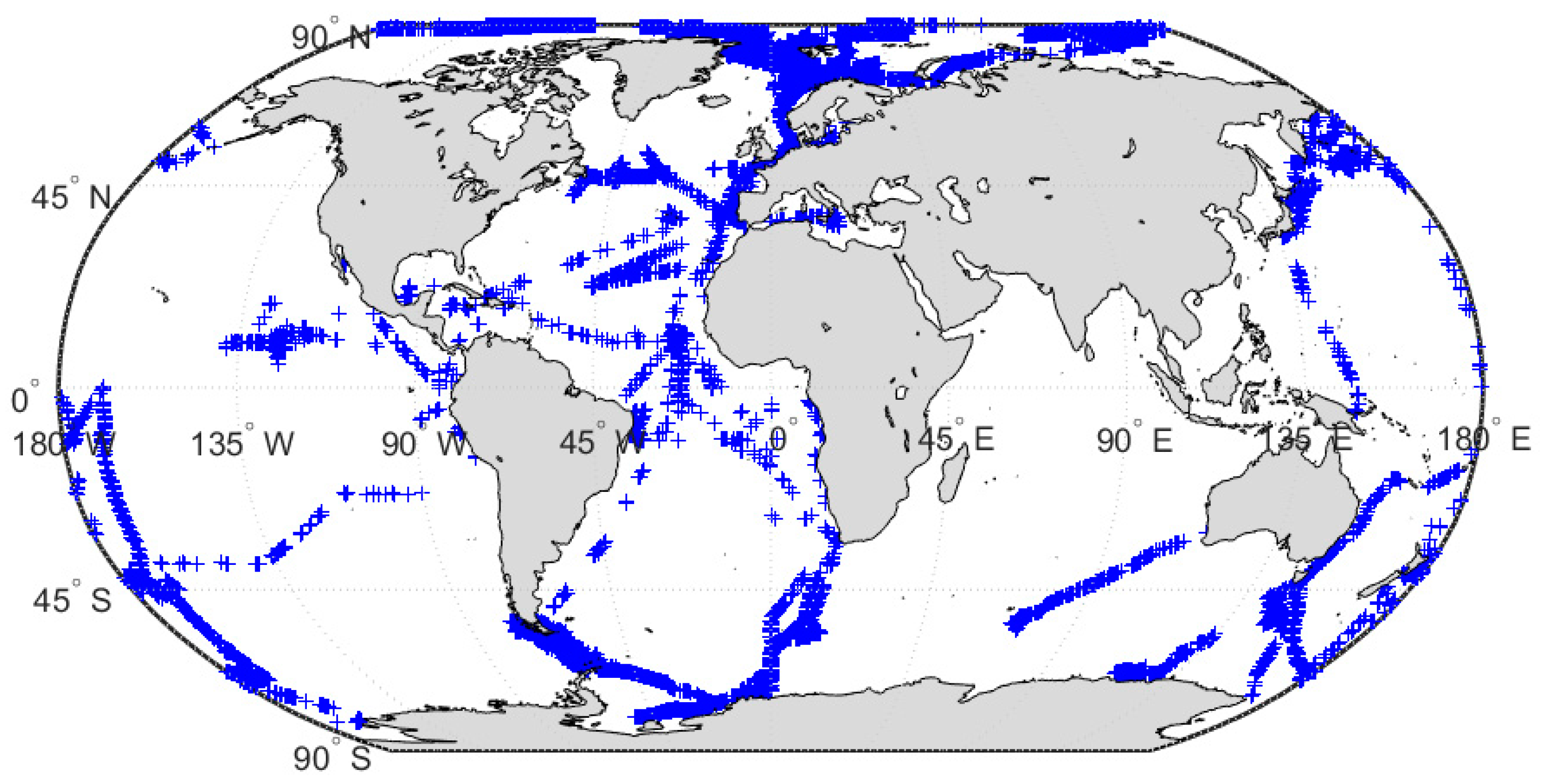
2.1. Data

IMERG fuses information from multiple sources, including satellite microwave and infrared precipitation estimates and ground gauge information. The IMERG algorithm uses several passive microwave (PMW) sensors to assemble and intercalibrate precipitation estimates. However, due to the limited sampling of PMW sensors on low-earth-orbit platforms, the gaps are filled by MW-adjusted IR estimates. As IMERG products are provided at 30 min temporal resolution, MW retrievals are obtained either from calibrated conical-scan microwave radiometer or cross-track-scan microwave retrieval, essentially from the one that is closer to the half-hour window. IR estimates are provided by various sensors (refer to [21] for more details). The IMERG algorithm is run twice in near-real time and once after monthly gauge data become available to generate the following multi-satellite products: (i) early, available ~4 h after the observation time allowing quick assessment for flood and landslide forecasts; (ii) late, available ~12 h after the observation time, mainly for agricultural applications like drought monitoring, crop yield forecasts, and crop production; and (iii) final, available ~2 months after observation for research applications. The data fields are provided by the NASA Precipitation Processing System (PPS) as global Level-3 gridded precipitation estimates (mm·h⁻¹) at the spatial/temporal resolution of 0.1°/30 min. In this study, the following data fields archived in each IMERG file are used: precipcal for the early, late, and final merged products, HQprecipitation for the MW component, and IRprecipitation for the IR component.

The GPM core satellite carries the dual-frequency precipitation radar operating at Ku-band (13.6 GHz) and Ka-band (35.5 GHz). DPR provides measurements that are spaced at ~5 km, over 245 km (at Ku-band) and 120 km (at Ka-band) wide swaths. The attenuation and loss of the radar signal along with precipitation phase still influence DPR observations, as in the TRMM Precipitation Radar [22,23,24,25], but these issues are addressed in the Level-2 DPR algorithm. The Level-3 DPR algorithm performs a spatial and temporal statistical processing to generate gridded products that cover the whole globe and are available at multiple temporal (hourly, daily and monthly) and spatial (0.25° and 0.50°) resolutions. In this work, the daily Level-3 product 3DPRD is used at its native spatial resolution of 0.25° and with a spatial coverage from 67° S to 67° N and from 180° W to 180° E. The data archived in the GRID/precipRateESurfMean data field are utilized in this study. IMERG uses Level-2 PMW precipitation retrievals trained by the 2BCMB (GMI+DPR) combined algorithm. For interpreting reflectivity profiles from DPR reflectivity observations, 2BCMB uses a different approach than the DPR algorithm to interpret the reflectivity profiles. Moreover, several levels of processing from the 2BCMB estimates to the Level-2 PMW, which adopts a Bayesian retrieval algorithm, to IMERG guarantees that the IMERG product is different from the 2BCMB precipitation on a scene-by-scene basis, although their long-term means will look similar as a result of the intercalibration [26].

Several research vessels (RV) have gathered precipitation data along with auxiliary atmospheric data as part of the OceanRAIN initiative over the Pacific and Atlantic Oceans since 2010. The mainstay of OceanRAIN is an optical disdrometer (the Eigenbrodt ODM470) coupled with an anemometer and a precipitation detector. The measuring volume is illuminated evenly along the cross section by an infrared light diode. The ODM470 records the light extinction caused by the passing hydrometeor in terms of activation voltage which is proportional to the cross-sectional area of the hydrometeor [27]. To obtain the particle size distribution, the hydrometeors are counted in a 60 s window and sorted in a bin size ranging from 0.04 mm to 22 mm. A particle size distribution is then used to derive precipitation phase, intensity, accumulation, and precipitation occurrence. Moreover, the installation height of ODM470 on RVs assures minimal splashing water effect on the measurements. Further details regarding the instrument and the OceanRAIN dataset can be found in Klepp et al. [28]. Figure 1 shows the ship tracks of the RVs collecting precipitation data during the 3-year study period (March 2014–February 2017).

Information regarding the sample size of precipitation data collected by each RV is presented in

Table 1. Data collected by each research vessel (RV) during the 3-year study period (March 2014–Feb 2017).

RV ID	Sample Size	# Cases with Rain > 0 mm·h−1	Time Series
Sonne-II	60,168	58,083	Nov 2014–Jan 2015
Roger	10,763	8469	Aug–Sep 2014
Polastern	445,635	233,349	Mar 2014–Oct 2016
Meteor	20,299	19,358	Mar 201–Mar 2016
Maria	27,083	23,954	Mar–Jun 2014
Investigator	54,814	32,671	Jan 2016–Feb 2017
World	4879	3860	Jan–Feb 2017
TOTAL	623,641	379,744	Mar 2014–Feb 2017

. The temporal resolution of the data is 1 min. The ODM470 instrument used in OceanRAIN can measure very light precipitation (from 0.01 mm·h⁻¹ to 0.09 mm·h⁻¹) unlike common gauges. As highlighted in Klepp et al. [29], when an insignificant number of particles is recorded, the measurement is flagged and assigned a value of 0.00 mm·h⁻¹. Moreover, to avoid unrealistic spikes, quality control is maintained through routine visual inspections. Seven RVs have acquired OceanRAIN data during the three years of analysis. Polastern has the longest time series and thus collected the largest numbers of samples, whereas World spans over two months only and shows the smallest sample size. Measurements from all RVs are merged together to facilitate the comparison with the IMERG products/components, resulting in a total of 623,641 samples over the 3-year period. Considering rain rates larger than 0 mm·h⁻¹, the sample size reduces to 379,744 during the same study period. IMERG, DPR, and OceanRAIN data are all matched to the daily temporal scale and to a regular cartesian grid at four different spatial resolutions (0.5°, 1°, 2° and 3°).

2.2. Spatio-Temporal Data Alignment

IMERG (both merged products and components), DPR, and OceanRAIN data have different native resolutions. Moreover, OceanRAIN data are not gridded, which also necessitates a spatial alignment to a common grid. IMERG (native resolution = 0.1°) and 3DPRD (native resolution = 0.25°) are mapped to a common 0.5° cartesian grid through simple spatial averaging. Then, all OceanRAIN measurements falling within each 0.5° grid box are averaged together. Both IMERG and OceanRAIN datasets are averaged temporally for every day during the 3-year study period to match the daily resolution of 3DPRD.

In order to investigate the impact of spatial resolution (i.e., grid box size) on our analysis, daily IMERG and 3DPRD data are upscaled to coarser resolutions (1°, 2°, and 3°) and compared to the OceanRAIN data. IMERG, 3DPRD, and OceanRAIN at these resolutions are generated by spatially averaging all the valid observations (including zeros) available within each grid box. Statistical metrics for the three collocated products are thus computed at a total of four spatial resolutions (0.5°, 1°, 2° and 3°) and at the daily time scale.

2.3. Performance Analysis

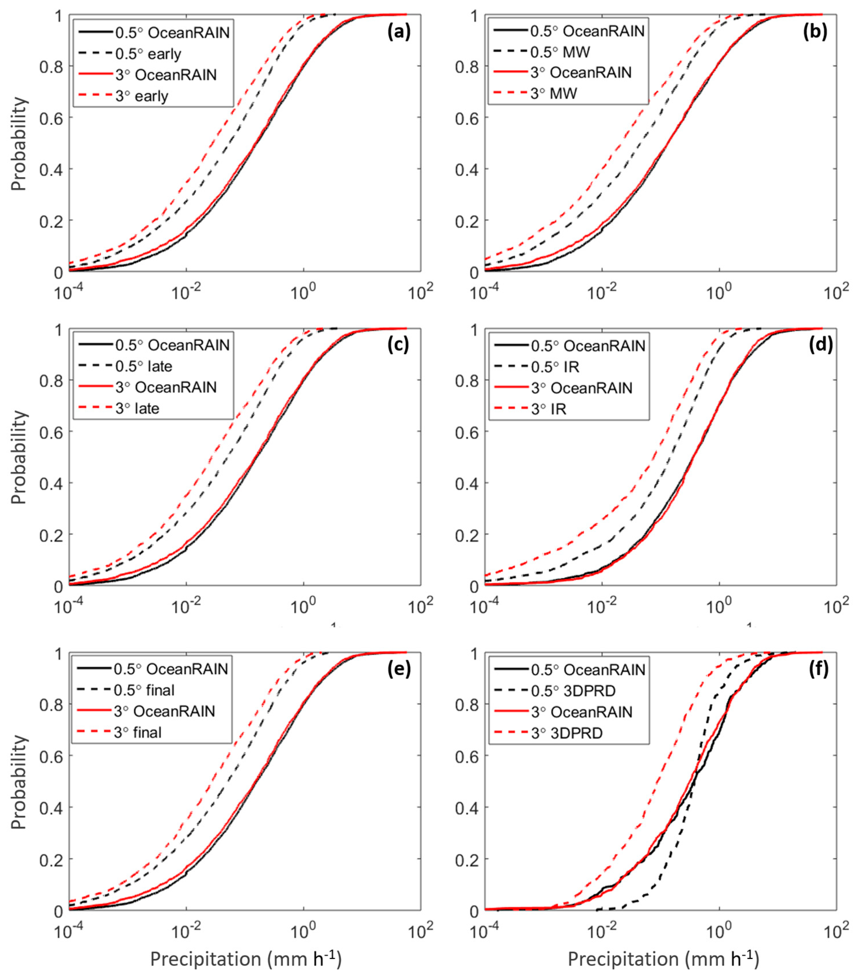
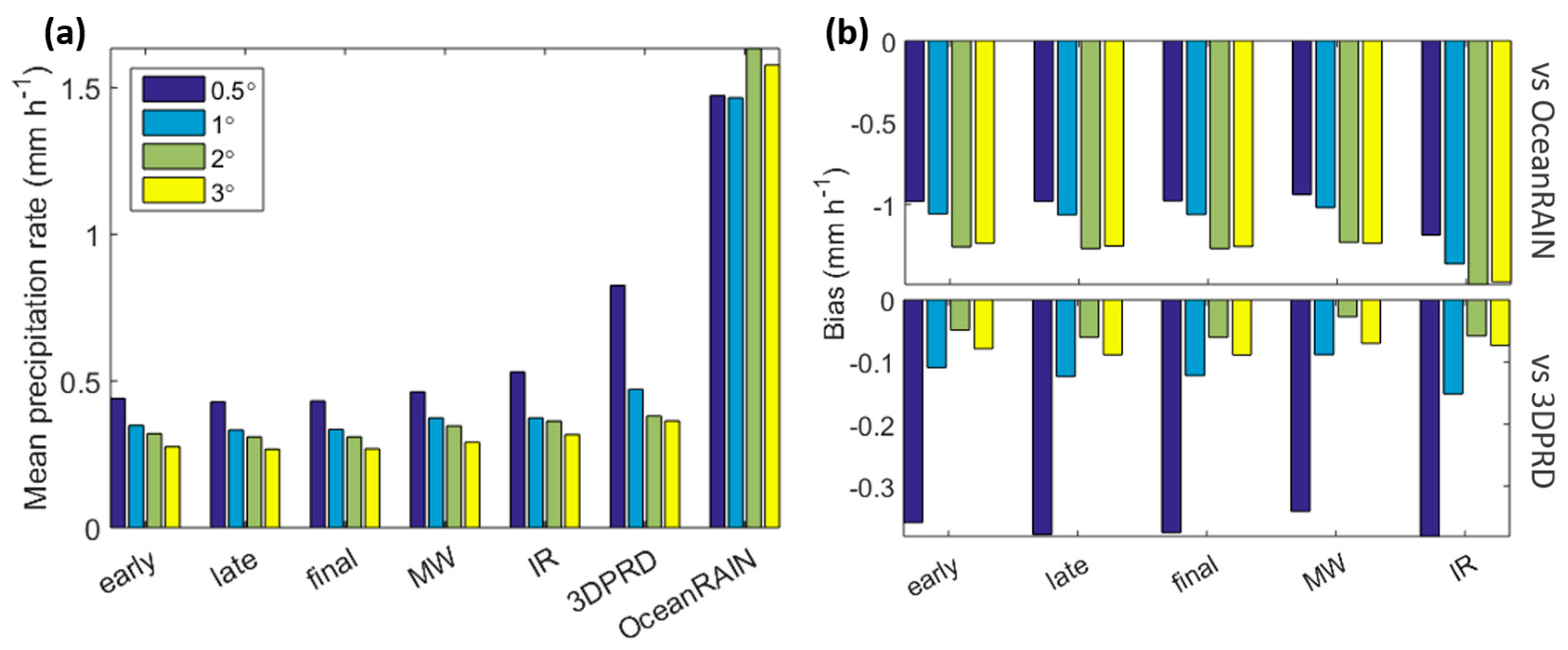
Categorical and continuous statistics allow characterization of systematic and random errors, which are both critical to evaluate and further improve precipitation retrieval algorithms, for instance through bias adjustment techniques. Both categorical and continuous statistics are used to assess the performance of the IMERG products/components against two references, i.e., OceanRAIN and 3DPRD. The rationale behind the use of two different reference datasets consists in the fact that over oceans there is no ideal benchmark for evaluating precipitation products that is continuously available both in time and space. A rain/no-rain threshold of 0.01 mm·h⁻¹ is used to compute categorical and continuous statistics. Categorical statistics include probability of detection (POD), success ratio (SR), critical success index (CSI), and the hit bias. Among the continuous statistics, correlation coefficient (CC), standard deviation (SD), and the root mean-square error (RMSE) are considered. Definitions and equations for each metric are reported in Appendix A, together with the contingency table on which the categorical statistics are based. All error metrics are computed at the daily scale for the four spatial resolutions.

Triple collocation is an alternative method for assessing the quality of a product without assuming a reference and the random errors are computed against an unknown truth [30,31,32,33,34,35,36]. This technique has been widely used in precipitation studies, although some studies showed that TCA is highly sensitive to its input configurations, including scale differences, time span under observation, and measurement triplets [37,38,39]. The method proposed by McColl et al. [31] is applied here to estimate RMSE and R² values of a specific precipitation product with the truth defined as:

$$X_i=X_i^{\prime }+{\epsilon }_i={\alpha }_i+{\beta }_{i}t+{\epsilon }_i$$

(1)

where $X_i(i\in \{1, 2, 3\})$ represents collocated measurement systems linearly related to the true value t with additive random errors ${\epsilon }_i$, whereas ${\alpha }_i$ and ${\beta }_i$ represent the least square intercepts and slopes, respectively. Assuming that the errors from each system have (i) zero mean, (ii) are mutually uncorrelated ($\mathrm{Cov}\left({\epsilon }_i, {\epsilon }_j\right)=0, i\ne j$), and (iii) orthogonal with respect to t ($\mathrm{Cov}({\epsilon }_i, t)$), the RMSE and coefficient of determination (R²) are computed as follows:

$$RMSE=\left[\begin{array}{c}\sqrt{Q_{11}-\frac{Q_{12}{Q}_{13}}{Q_{23}}}\\ \sqrt{Q_{22}-\frac{Q_{12}{Q}_{23}}{Q_{13}}}\\ \sqrt{Q_{33}-\frac{Q_{12}{Q}_{23}}{Q_{12}}}\end{array}\right]$$

(2)

$$R^2=\left[\begin{array}{c}\frac{Q_{12}{Q}_{13}}{Q_{11}{Q}_{23}}\\ \frac{Q_{12}{Q}_{23}}{Q_{13}{Q}_{22}}\\ \frac{Q_{13}{Q}_{23}}{Q_{12}{Q}_{33}}\end{array}\right]$$

(3)

where $Q_{ij}=\mathrm{Cov}\left(X_i, X_j\right)$ and Cov represents the covariance matrix.

We applied TCA by aggregating daily data at different spatial resolutions (0.5°, 1°, 2° and 3°) over the 3-year period and by selecting instances when and where all three datasets have precipitation rates ≥ 0.01 mm·h⁻¹. TCA is applied to the following triplets of precipitation products: (1) early-3DPRD-OceanRAIN (Triplet A); (2) late-3DPRD-OceanRAIN (Triplet B); (3) final-3DPRD-OceanRAIN (Triplet C); (4) MW-3DPRD-OceanRAIN (Triplet D); and (5) IR-3DPRD-OceanRAIN (Triplet E). R² and the RMSE are then computed for each triplet.

3. Results

As a first step to investigate the datasets considered in this study, the probability density functions (PDFs) of each of the six daily precipitation products at 0.5°, 1°, 2° and 3° spatial resolutions are investigated (Figure 2). At the finer scale (0.5°), 3DPRD demonstrates a sharp distribution concentrated around small precipitation rates (<0.01 mm·h⁻¹), whereas IR reveals the most uniform distribution among all datasets. The MW component and the merged products have all similar distributions that are close to the one of OceanRAIN. Coarser resolutions result in flatter 3DPRD distributions that get closer to the other IMERG products. In the IR distributions, the density of low precipitation rates becomes larger at coarser resolutions. Other IMERG products maintain similar distributions when moving from finer to coarser resolutions, except for IMERG early, which flattens out significantly at 3°. The distribution of OceanRAIN is similar across the four resolutions, albeit slight variations at small rain rates (<0.01 mm·h⁻¹).

In order to further investigate the performance of the satellite-based precipitation products with respect to the ground reference, cumulative distribution functions (CDFs) of daily IMERG products and 3DPRD are compared to the CDF of OceanRAIN at 0.5° and 3° resolutions (Figure 3). All IMERG products and components show an overall underestimation with respect to OceanRAIN, both at finer and coarser spatial resolutions. This underestimation increases when moving from the finer to the coarser resolution. When analyzing the CDF of 3DPRD at 0.5°, we observe an overestimation of precipitation rates ranging between 0.01 mm·h⁻¹ and 0.9 mm·h⁻¹ and an underestimation at larger rain rates. However, at the coarser resolution, 3DPRD consistently underestimates the reference, similarly to the other satellite-based products.

As mentioned above, the performance of the IMERG products and components is further investigated against two different references: OceanRAIN and 3DPRD. The performance metrics considered in this work are illustrated in Figure 4 and Figure 5 in terms of performance and Taylor diagrams [40,41]. The performance diagram displays categorical statistics such as probability of detection (POD), success ratio (SR), critical success index (CSI), and hit bias. The upper right corner of the diagram represents the perfect score with POD, SR, CSI and hit bias approaching 1. Both performance and Taylor’s diagrams are presented at the four different resolutions: 0.5° (a–b); 1° (c–d); 2° (e–f); and 3° (g–h) for each one of the five IMERG precipitation products. The left panels in each Figure present results for OceanRAIN as reference, whereas the right panels show 3DPRD as the reference.

By analyzing the performance diagrams in Figure 4, we observe that, overall, IR is the only product whose statistics are markedly different from the other products, which are closely packed together in the diagrams. POD is just below 0.80 for all IMERG products except for IR, which has a POD slightly greater than 0.80 with OceanRAIN as reference. This suggests that all products have a good ability of detecting precipitation (i.e., ~80% of the times that OceanRAIN detects rain, the satellite product agrees). SR on the other hand is the lowest for IR (~0.55) and higher for other products (~0.65). Likewise, the hit bias and CSI are respectively around 1.50 and 0.50 for IR and 1.30 and 0.55 for the other products at 0.5° resolution, when compared to OceanRAIN. The performance metrics show minimal changes with spatial resolutions: SR and CSI exhibit slight improvements at coarser resolutions, whereas POD and hit bias do not show any dependence on the spatial scale.

By analyzing the performance diagrams with 3DPRD as reference (presented in the right panels in Figure 4), we observe that the POD is much lower (0.35–0.65) than in the previous case (when OceanRAIN was taken as benchmark) and that it shows larger variability across different spatial resolutions. However, the SR is not influenced by changes in the spatial resolution and ranges between 0.70 and 0.80 for all products. CSI and the hit bias also manifest improvement at coarser spatial resolutions with values increasing from 0.35 to 0.55 for CSI and from 0.50 to 0.85 for the hit bias. CSI may not always be a reliable indicator because of its dependence on frequency of events. Specifically, it may increase with resolution because of its inherent bias with event frequency. However, CSI is a valid indicator of the relative performance of various algorithms [42]. Interestingly, the difference in performance between IR and other IMERG products follow a very similar pattern for both references.

The Taylor diagrams in Figure 5 present continuous statistics such as correlation (CC), normalized standard deviation (SD), and root-mean square error (RMSE), where RMSE is expressed as a function of CC and SD. A normalized version of the Taylor diagrams, in which the SD and RMSE are normalized by the standard deviation of the reference, is considered here to provide a better measure of the relative performances of the satellite-based precipitation products [41]. The perfect scores are 0 for RMSE and 1 for CC and SD. Similarly to the categorical scores, continuous statistics are computed at four different resolutions: 0.5° (a–b); 1° (c–d); 2° (e–f); and 3° (g–h) spatial resolutions. The left panels correspond to OceanRAIN taken as the reference, whereas the right panels consider 3DPRD as the reference. At 0.5°, the correlation coefficient between all the IMERG products and OceanRAIN is 0.20, except for the IR component, which exhibits minimal CC (0.05). CC doubles for all the products at 1° spatial resolution (5c), including IR, depicting a CC of 0.4. RMSE follows a very similar trend as CC with changing resolutions. Specifically, RMSE shows the lowest values at 1° (0.80), whereas it is 1 for the other resolutions. At 0.5° and 1° SD is 0.25 for all IMERG products and decreases to 0.1 at 2° and 3° resolutions. Overall, the continuous statistics for all IMERG products appear to converge at a single value at 2° and 3°.

Continuous statistics with 3DPRD used as a reference exhibit more pronounced variability at coarser spatial scales. CC changes from 0.40 at 0.5° and 1° resolutions to 0.45 at 2°, and to 0.30 at 3° resolution. RMSE shows values of 0.80 at 0.5° and 2° resolutions and of 1 at 1° and 3° resolutions for all IMERG products. SD moves closer to the reference value (SD = 1) as the spatial resolution goes up from 0.35 (at 0.5°) to 0.75 (at 2°), but it falls back to 0.50 at 3°. Among all IMERG products, the MW estimates exhibit the best continuous statistics when evaluated against 3DPRD.

Since the categorical and continuous statistics do not provide a definitive answer to what reference should be used to evaluate the IMERG products and components, a triple collocation analysis is adopted here as an alternative method to investigate random errors associated with the products of interest.

Table 2. RMSE (in mm·h⁻¹) and R² from TCA for five precipitation product triplets at four spatial resolutions (0.5°, 1°, 2°, 3°).

Triplet ID	Products	RMSE (mm·h−1) 0.5°, 1°, 2°, 3°	R2 0.5°, 1°, 2°, 3°
A	early	0.35, 0.30, 0.22, 0.21	0.50, 0.45, 0.67, 0.53
	3DPRD	1.05, 0.50, 0.40, 0.53	0.32, 0.37, 0.36, 0.19
	OceanRAIN	2.15, 1.61, 3.20, 2.88	0.07, 0.38, 0.05, 0.08
B	late	0.33, 0.29, 0.22, 0.21	0.48, 0.43, 0.62, 0.50
	3DPRD	1.07, 0.49, 0.40, 0.53	0.27, 0.40, 0.38, 0.20
	OceanRAIN	2.14, 1.64, 3.18, 2.88	0.08, 0.35, 0.05, 0.08
C	final	0.32, 0.28, 0.23, 0.20	0.50, 0.43, 0.61,0.51
	3DPRD	1.09, 0.49, 0.40, 0.52	0.26, 0.40, 0.37, 0.21
	OceanRAIN	2.12, 1.62, 3.22, 2.90	0.08, 0.35, 0.05, 0.07
D	MW	0.36, 0.32, 0.24, 0.22	0.62, 0.47, 0.71, 0.53
	3DPRD	1.02, 0.49, 0.40, 0.53	0.37, 0.42, 0.37, 0.19
	OceanRAIN	2.21, 1.68, 3.32, 2.92	0.06, 0.33, 0.05, 0.08
E	IR	0.59, 0.38, 0.29, 0.23	0.04, 0.31, 0.63, 0.48
	3DPRD	1.86, 0.61, 0.48, 0.61	0.01, 0.31, 0.31, 0.12
	OceanRAIN	2.62, 1.87, 3.84, 3.26	0.00, 0.37, 0.04, 0.09

summarizes the TCA results for the five triplets for each one of the IMERG products and components, when 3DPRD and OceanRAIN are used as the other two measurements. The RMSE and R² values obtained from TCA are compared at the four spatial resolutions. Among the three precipitation measurements in each triplet, the IMERG products consistently exhibit the higher correlations and lower RMSE values.

Figure 6a presents mean values of all precipitation products at four spatial resolutions along the study time series, whereas Figure 6b shows the overall bias (mm·h⁻¹) of each satellite product, defined as follows:

$$Bias={\mathsf{\mu }}_{\mathrm{Sat}}-{\mathsf{\mu }}_{Ref}$$

(4)

where μ_Ref is the mean precipitation of either OceanRAIN (top panel) or 3DPRD (bottom panel), and μ_Sat represents the mean precipitation of each IMERG product/component. Precipitation mean values and biases are computed for collocated products using a threshold of 0.01 mm·h⁻¹.

The precipitation mean of all satellite products decreases when moving to coarser resolutions (from 0.5° to 3°), likely due to the inclusion of more pixels where no precipitation occurs. However, this is not the case for OceanRAIN, since not as many more observations as in the case of the gridded products are included when increasing resolution. In terms of bias, all IMERG products show larger bias when OceanRAIN is used as a reference as opposed to 3DPRD, which is expected due to the inherent different nature of satellite-based retrievals and track-based observations. For the same reason, biases between the IMERG products and OceanRAIN tend to increase when resolution gets coarser, whereas IMERG biases with respect to 3DPRD decrease with coarser resolution because of the smoothing effect of the spatial aggregation. This is a critical point that should be considered when choosing a satellite-based reference versus a track-based one for evaluating IMERG products over oceans.

TCA also allows us to compare the two references used in the previous analyses against an unknown truth. 3DPRD consistently outperforms OceanRAIN in terms of both R² and RMSE at all spatial resolutions. A comparison across the spatial resolutions reveals a very interesting pattern, that is, R² values are consistently higher for 3DPRD, as already anticipated by the Taylor diagrams. In terms of RMSE, mean values for OceanRAIN across all the triplets are 2.25 mm·h⁻¹, 1.68 mm·h⁻¹, 3.35 mm·h⁻¹, and 2.97 mm·h⁻¹ at 0.50°, 1°, 2° and 3° resolution, respectively. Mean RMSE value for 3DPRD across all the triplets are 1.22 mm·h⁻¹ (0.50°), 0.52 mm·h⁻¹ (1°), 2.08 mm·h⁻¹ (2°) and 0.54 mm·h⁻¹ (3°).

In terms of triplets that consider IMERG products and components, Triplets A-D show comparable performances in terms of both RMSE and R², with Triplet D (the one including the MW component) showing the lowest RMSE and the largest R² and Triplet E (the one including the IR component) showing the worst performance at all spatial resolutions. It is worth noting that the TCA assumption of linear dependence among the datasets is not met for the 0.50° resolution for the IR component, which leads to R² values close to 0 for all the measurements in Triplet E.

4. Discussion

More than 75% of the global rain occurs over oceans, thus necessitating reliable measurements over oceans for better understanding global atmospheric and hydrological processes. The launch of precipitation-focused satellite missions (i.e., TRMM and GPM) in the past few decades has provided the opportunity to estimate precipitation at fine spatial/temporal resolutions over oceans, where surface observations are sparse and often influenced by wind speed and direction and by the stability of the measuring platform [8]. Nevertheless, the true capability of these satellite precipitation estimates over oceans is closely linked to the quantification of the uncertainties associated with them.

In this context, this study assesses the performance of the latest V05 IMERG products and components over oceans. Two independent references (OceanRAIN and 3DPRD) are used to evaluate the products at four spatial resolutions and daily temporal scale over a 3-year study period. All IMERG products show comparable precipitation distributions, except for the IR estimates. An overall underestimation by all IMERG products and 3DPRD against the OceanRAIN is observed for the analysis period, which corroborates results from other studies where moored buoys were used as a reference to evaluate satellite rainfall estimates [13]. Precipitation rates lower than 0.1 mm·h⁻¹ dominate the distributions in all products and are more pronounced in 3DPRD estimates. The OceanRAIN PDF appears to migrate closer to the IR PDF as we move to coarser resolutions, which can be attributed to the IR sampling. Specifically, IR has good sampling and despite the noise, the IR mean should converge to the mean of the MW with sufficient spatial/temporal averaging, which could be the case here. The reader should note that the IR field provided in the half hour IMERG file may not have been the one used in the merger with that half hour’s satellite estimates. In IMERG versions 03 through 05, the next half hour’s IR is used to merge with the current half hour’s satellite estimates since it tends to exhibit the highest correlation.

The performance of IMERG products and components is assessed by using a plethora of statistical metrics to provide a comprehensive analysis of their associated uncertainty and errors. Among all products, IR estimates perform worst in terms of CC, SD, and RMSE. However, in terms of POD, the IR component tends to depict slightly improved values as compared to other IMERG products against both references. The IMERG products follow IR in terms of rain detection because IR is the only high-frequency observation contributing to the IMERG algorithm, whereas the MW component is obtained from either calibrated conical-scan microwave radiometer retrievals or cross-track-scan microwave sounder retrievals, whichever is closer to the half-hour window. The IR-based product is estimated indirectly via cloud top temperature measurements. Oceans are commonly characterized by dense cloud cover over tropical and temperate regions [43]. The increased POD for IR estimates could be attributed to the fact that the data collected by RVs are mostly in the tropical and temperate regions typically receiving more convective rainfall, which is well detected by IR sensors [44]. On the contrary, the MW component performs better than the other components in terms of both categorical and continuous statistics, which is in line with past studies conducted using buoys as a reference [13,45]. As this study does not distinguish the Pacific Ocean from the Atlantic Ocean, the performance over a specific region cannot be inferred. However, previous studies suggest inconsistencies in POD, SR, CC, and RMSE for satellite estimates across the western and eastern Pacific and Atlantic Oceans [45,46,47].

3DPRD has the potential to be a very useful reference because of its global availability at all times as opposed to OceanRAIN that provides very limited spatio-temporal measurements. In general, while performance metrics are slightly better when OceanRAIN is used as reference to evaluate the IMERG products, the continuous statistics are clearly better when 3DPRD is adopted. This may be attributed to the similar nature of satellite-based products and to the pixel-to-pixel comparison (with respect to the point-to-pixel comparison used in the OceanRain analysis). Although the along-track averaged precipitation of OceanRAIN provides better representation of the areal extent of satellite measurements, the track-to-area difference could be minimized by statistical adjustments as proposed by Burdanowitz et al. [20]. Overall, this does not point to a conclusive evidence as to which reference (OceanRAIN or 3DPRD) should be used for validating the IMERG products. Thus, using an unknown truth-based analysis, such as TCA, is the recommended approach to evaluate random errors associated with satellite-based products over oceans. Theoretically, TCA provides error variance without assuming one of the observations as ground truth. The main assumption of TCA is that three products have mutually independent errors. The results are biased to some extent when two remotely sensed observations are used in the triplets. TCA shows a similar picture in terms of the relative performance of the IMERG products and components with respect to each other as observed in other performance metrics (e.g., RMSE, SD, and CC). Among all products analyzed here, IMERG final shows the lowest RMSE with respect to the truth, followed by late, early, MW, IR, 3DPRD, and OceanRAIN. The R² is relatively higher for the IMERG products/components than the one of 3DPRD and OceanRAIN. In TCA, the performance of OceanRAIN is better at 1° resolution compared to other resolutions. However, the satellite-based products do not show this behavior. This can possibly be attributed to the influence of track-to-area averaging, i.e., the areal nature of satellite products vs the track structure of OceanRAIN. This is an interesting point that should be investigated further in future studies.

TCA clearly confirms that 3DPRD performs consistently better than OceanRAIN, as also shown by the continuous error metrics. Khan et al. [48] demonstrated that IR estimates are affected by the largest systematic and random errors over land compared to the other IMERG products and components and their improvement could be critical to enhance the merged products. The findings over ocean also point to larger errors in IR estimates over oceans, thus providing an opportunity to improve the merged products also over oceans.

Using OceanRAIN as a reference for evaluating GPM-based products has its own limitations. First, although OceanRAIN data are available since 2010, only a few years overlap with the GPM mission. Second, measurements are spatially sparse and sample sizes are small at coarser temporal resolutions. At this point mapping errors spatially is not possible because of the short length of the time series, but additional validation analysis should be performed when longer time series of OceanRAIN and GPM estimates will be available. A rain/no-rain threshold value is set to 0.01 mm·h⁻¹ for computing categorical and continuous statistics. This threshold may not be ideal for evaluating satellite products at their native resolutions, as it is below the minimum detection limit of most spaceborne instruments. However, a higher threshold would result in a reduced sample size, consequently resulting in less robust conclusions. Future work should investigate the impact of this threshold on the validation analysis.

5. Conclusions

This study evaluates the performance of Level-3 GPM gridded products over oceans using 3DPRD and OceanRAIN as potential references. Similarly, this methodology could be applied to other new generation satellite-based precipitation products, such as the Global Satellite Mapping of Precipitation (GSMaP) product by JAXA [49]. The quasi-global availability of DPR-based measurements makes it a unique reference where and when a surface-based reference is not available. Moreover, compared to passive remote sensors such as passive microwave and infrared sensors, DPR offers more accurate precipitation estimates. IR estimates exhibit margin for improvement over oceans, which in turn could lead to reduction in errors in the merged products. Future extension of this work could include alternate independent precipitation datasets such as buoys and model reanalysis for the TCA. Future studies should investigate error sources and attempt to separate error components (systematic and random), which is extremely important to implement improvements in satellite precipitation algorithms.

References

1. Hong, Y.; Adler, R.F.; Negri, A.; Huffman, G.J. Flood and landslide applications of near real-time satellite rainfall products. Nat. Hazards 2007, 43, 285–294. [Google Scholar] [CrossRef] [Green Version]
2. Hossain, F.; Anagnostou, E.N. Assessment of current passive-microwave- and infrared-based satellite rainfall remote sensing for flood prediction. J. Geophys. Res. Atmos. 2004, 109, D07102. [Google Scholar] [CrossRef]
3. Johnson, G.E.; Achutuni, V.R.; Thiruvengadachari, S.; Kogan, F. The Role of NOAA Satellite Data in Drought Early Warning and Monitoring: Selected Case Studies. In Drought Assessment, Management, and Planning: Theory and Case Studies; Natural Resource Management and Policy; Springer: Boston, MA, USA, 1993; pp. 31–47. ISBN 978-1-4613-6416-0. [Google Scholar]
4. Krajewski, W.F.; Anderson, M.C.; Eichinger, W.E.; Entekhabi, D.; Hornbuckle, B.K.; Houser, P.R.; Katul, G.G.; Kustas, W.P.; Norman, J.M.; Peters-Lidard, C. A remote sensing observatory for hydrologic sciences: A genesis for scaling to continental hydrology. Water Resour. Res. 2006, 42. [Google Scholar] [CrossRef] [Green Version]
5. Hou, A.Y.; Kakar, R.K.; Neeck, S.; Azarbarzin, A.A.; Kummerow, C.D.; Kojima, M.; Oki, R.; Nakamura, K.; Iguchi, T. The global precipitation measurement mission. Bull. Am. Meteorol. Soc. 2014, 95, 701–722. [Google Scholar] [CrossRef]
6. Kidd, C.; Becker, A.; Huffman, G.J.; Muller, C.L.; Joe, P.; Skofronick-Jackson, G.; Kirschbaum, D.B. So, how much of the Earth’s surface is covered by rain gauges? Bull. Am. Meteorol. Soc. 2017, 98, 69–78. [Google Scholar] [CrossRef]
7. Bumke, K.; Fennig, K.; Strehz, A.; Mecking, R.; Schröder, M. HOAPS precipitation validation with ship-borne rain gauge measurements over the Baltic Sea. Tellus Dyn. Meteorol. Oceanogr. 2012, 64, 18486. [Google Scholar] [CrossRef]
8. Skofronick-Jackson, G.; Kirschbaum, D.; Petersen, W.; Huffman, G.; Kidd, C.; Stocker, E.; Kakar, R. The Global Precipitation Measurement (GPM) mission’s scientific achievements and societal contributions: Reviewing four years of advanced rain and snow observations. Q. J. R. Meteorol. Soc. 2018, 144, 27–48. [Google Scholar] [CrossRef]
9. Anagnostou, E.N.; Krajewski, W.F.; Smith, J. Uncertainty quantification of mean-areal radar-rainfall estimates. J. Atmos. Ocean. Technol. 1999, 16, 206–215. [Google Scholar] [CrossRef]
10. Kent, E.; Hall, A.D.; Leader, V.T.T. The voluntary observing ship (VOS) scheme. In Proceedings of the 2010 AGU Ocean Sciences Meeting, Portland, OR, USA, 22–26 February 2010; American Geophysical Union: Washington, DC, USA. [Google Scholar]
11. Smith, S.R.; Rettig, J.; Rolph, J.; Hu, J.; Kent, E.C.; Schulz, E.; Verein, R.; Rutz, S.; Paver, C. The data management system for the Shipboard Automated Meteorological and Oceanographic System (SAMOS) initiative. In Proceedings of the OceanObs’ 09: Sustained Ocean Observations and Information for Society Conference, Venice, Italy, 21–25 September 2009; Volume 2. [Google Scholar]
12. Hayes, S.P.; Mangum, L.J.; Picaut, J.; Sumi, A.; Takeuchi, K. TOGA-TAO: A moored array for real-time measurements in the tropical Pacific Ocean. Bull. Am. Meteorol. Soc. 1991, 72, 339–347. [Google Scholar] [CrossRef]
13. Serra, Y.L. Precipitation measurements from the Tropical Moored Array: A review and look ahead. Q. J. R. Meteorol. Soc. 2018, 144, 221–234. [Google Scholar] [CrossRef]
14. Bowman, K.P. Comparison of TRMM precipitation retrievals with rain gauge data from ocean buoys. J. Clim. 2005, 18, 178–190. [Google Scholar] [CrossRef]
15. Serra, Y.L.; McPhaden, M.J. In situ observations of diurnal variability in rainfall over the tropical Pacific and Atlantic Oceans. J. Clim. 2004, 17, 3496–3509. [Google Scholar] [CrossRef]
16. Serra, Y.L.; McPhaden, M.J. Multiple time-and space-scale comparisons of ATLAS buoy rain gauge measurements with TRMM satellite precipitation measurements. J. Appl. Meteorol. 2003, 42, 1045–1059. [Google Scholar] [CrossRef]
17. Levizzani, V.; Kidd, C.; Aonashi, K.; Bennartz, R.; Ferraro, R.R.; Huffman, G.J.; Roca, R.; Turk, F.J.; Wang, N.-Y. The activities of the International Precipitation Working Group. Q. J. R. Meteorol. Soc. 2018, 144, 3–15. [Google Scholar] [CrossRef]
18. Klepp, C. The oceanic shipboard precipitation measurement network for surface validation—OceanRAIN. Atmos. Res. 2015, 163, 74–90. [Google Scholar] [CrossRef]
19. Kucera, P.; Klepp, C. Validation of High Resolution IMERG Satellite Precipitation over the Global Oceans using OceanRAIN. In Proceedings of the EGU General Assembly Conference Abstracts, Vienna, Austria, 23–28 April 2017; Volume 19, p. 11794. [Google Scholar]
20. Burdanowitz, J.; Klepp, C.; Bakan, S.; Buehler, S.A. Towards an along-track validation of HOAPS precipitation using OceanRAIN optical disdrometer data over the Atlantic Ocean. Q. J. R. Meteorol. Soc. 2018, 144, 235–254. [Google Scholar] [CrossRef]
21. Huffman, G.J.; Bolvin, D.T.; Braithwaite, D.; Hsu, K.; Joyce, R.; Xie, P.; Yoo, S.-H. NASA Global Precipitation Measurement (GPM) Integrated Multi-Satellite Retrievals for GPM (IMERG); Algorithm Theoretical Basis Document (ATBD) Version 4.5; NASA: Greenbelt, MD, USA, 2015; 30p.
22. Iguchi, T.; Kozu, T.; Meneghini, R.; Awaka, J.; Okamoto, K. Rain-profiling algorithm for the TRMM precipitation radar. J. Appl. Meteorol. 2000, 39, 2038–2052. [Google Scholar] [CrossRef]
23. Iguchi, T.; Kozu, T.; Kwiatkowski, J.; Meneghini, R.; Awaka, J.; Okamoto, K. ’ichi Uncertainties in the rain profiling algorithm for the TRMM precipitation radar. J. Meteorol. Soc. Jpn. Ser. II 2009, 87, 1–30. [Google Scholar] [CrossRef]
24. Wolff, D.B.; Fisher, B.L. Comparisons of instantaneous TRMM ground validation and satellite rain-rate estimates at different spatial scales. J. Appl. Meteorol. Climatol. 2008, 47, 2215–2237. [Google Scholar] [CrossRef]
25. Yang, S.; Olson, W.S.; Wang, J.-J.; Bell, T.L.; Smith, E.A.; Kummerow, C.D. Precipitation and latent heating distributions from satellite passive microwave radiometry. Part II: Evaluation of estimates using independent data. J. Appl. Meteorol. Climatol. 2006, 45, 721–739. [Google Scholar] [CrossRef]
26. Petersen, W.; Kirstetter, P.; Wolff, D.; Kidd, C.; Tokay, A.; Chandrasekar, V.; Gatlin, P.; Tan, J.; Grecu, M.; Huffman, G. GPM Level 1 Science Requirements: Science and Performance Viewed from the Ground. In Proceedings of the 8th International Precipitation Working Group Workshop, Bologna, Italy, 3–7 October 2016. [Google Scholar]
27. Lempio, G.E.; Bumke, K. Measurements of solid precipitation with an optical disdrometer. Int. BALTEX Secr. Publ. Ser. 2007, 38, 123–124. [Google Scholar] [CrossRef]
28. Klepp, C.; Michel, S.; Protat, A.; Burdanowitz, J.; Albern, N.; Louf, V.; Bakan, S.; Dahl, A.; Thiele, T. Ocean Rainfall and Ice-Phase Precipitation Measurement Network—OceanRAIN-M; World Data Center for Climate (WDCC) at DKRZ: Hamburg, Germany, 2017. [Google Scholar]
29. Klepp, C.; Michel, S.; Protat, A.; Burdanowitz, J.; Albern, N.; Kähnert, M.; Dahl, A.; Louf, V.; Bakan, S.; Buehler, S.A. OceanRAIN, a new in-situ shipboard global ocean surface-reference dataset of all water cycle components. Sci. Data 2018, 5, 180122. [Google Scholar] [CrossRef] [PubMed]
30. Roebeling, R.A.; Wolters, E.L.A.; Meirink, J.F.; Leijnse, H. Triple collocation of summer precipitation retrievals from SEVIRI over Europe with gridded rain gauge and weather radar data. J. Hydrometeorol. 2012, 13, 1552–1566. [Google Scholar] [CrossRef]
31. McColl, K.A.; Vogelzang, J.; Konings, A.G.; Entekhabi, D.; Piles, M.; Stoffelen, A. Extended triple collocation: Estimating errors and correlation coefficients with respect to an unknown target. Geophys. Res. Lett. 2014, 41, 6229–6236. [Google Scholar] [CrossRef] [Green Version]
32. Alemohammad, S.H.; McColl, K.A.; Konings, A.G.; Entekhabi, D.; Stoffelen, A. Characterization of precipitation product errors across the United States using multiplicative triple collocation. Hydrol. Earth Syst. Sci. 2015, 19, 3489–3503. [Google Scholar] [CrossRef] [Green Version]
33. Stoffelen, A. Toward the true near-surface wind speed: Error modeling and calibration using triple collocation. J. Geophys. Res. Oceans 1998, 103, 7755–7766. [Google Scholar] [CrossRef] [Green Version]
34. Gruber, A.; Su, C.-H.; Zwieback, S.; Crow, W.; Dorigo, W.; Wagner, W. Recent advances in (soil moisture) triple collocation analysis. Int. J. Appl. Earth Obs. Geoinf. 2016, 45, 200–211. [Google Scholar] [CrossRef]
35. Chakraborty, A.; Kumar, R.; Stoffelen, A. Validation of ocean surface winds from the OCEANSAT-2 scatterometer using triple collocation. Remote Sens. Lett. 2013, 4, 84–93. [Google Scholar] [CrossRef]
36. Dorigo, W.; Scipal, K.; Parinussa, R.M.; Liu, Y.Y.; Wagner, W.; De Jeu, R.A.; Naeimi, V. Error Characterisation of Global Active and Passive Microwave Soil Moisture Data Sets. Hydrol. Earth Syst. Sci. 2010, 14, 2605–2616. [Google Scholar] [CrossRef]
37. Loew, A.; Schlenz, F. A dynamic approach for evaluating coarse scale satellite soil moisture products. Hydrol. Earth Syst. Sci. 2011, 15, 75–90. [Google Scholar] [CrossRef] [Green Version]
38. Zwieback, S.; Scipal, K.; Dorigo, W.; Wagner, W. Structural and statistical properties of the collocation technique for error characterization. Nonlinear Process. Geophys. 2012, 19, 69–80. [Google Scholar] [CrossRef] [Green Version]
39. Massari, C.; Crow, W.; Brocca, L. An assessment of the performance of global rainfall estimates without ground-based observations. Hydrol. Earth Syst. Sci. 2017, 21, 4347–4361. [Google Scholar] [CrossRef] [Green Version]
40. Roebber, P.J. Visualizing multiple measures of forecast quality. Weather Forecast. 2009, 24, 601–608. [Google Scholar] [CrossRef]
41. Taylor, K.E. Summarizing multiple aspects of model performance in a single diagram. J. Geophys. Res. Atmos. 2001, 106, 7183–7192. [Google Scholar] [CrossRef] [Green Version]
42. Schaefer, J.T. The critical success index as an indicator of warning skill. Weather Forecast. 1990, 5, 570–575. [Google Scholar] [CrossRef]
43. NASA GISS: Science Briefs: Cloud Climatology: Distribution and Character of Clouds. Available online: https://www.giss.nasa.gov/research/briefs/rossow_01/distrib.html (accessed on 16 November 2018).
44. Adler, R.F.; Negri, A.J. A satellite infrared technique to estimate tropical convective and stratiform rainfall. J. Appl. Meteorol. 1988, 27, 30–51. [Google Scholar] [CrossRef]
45. Sapiano, M.R.P.; Arkin, P.A. An intercomparison and validation of high-resolution satellite precipitation estimates with 3-hourly gauge data. J. Hydrometeorol. 2009, 10, 149–166. [Google Scholar] [CrossRef]
46. Huffman, G.J.; Bolvin, D.T.; Nelkin, E.J.; Wolff, D.B.; Adler, R.F.; Gu, G.; Hong, Y.; Bowman, K.P.; Stocker, E.F. The TRMM multisatellite precipitation analysis (TMPA): Quasi-global, multiyear, combined-sensor precipitation estimates at fine scales. J. Hydrometeorol. 2007, 8, 38–55. [Google Scholar] [CrossRef]
47. Kidd, C.; Huffman, G. Global precipitation measurement. Meteorol. Appl. 2011, 18, 334–353. [Google Scholar] [CrossRef] [Green Version]
48. Khan, S.; Maggioni, V.; Kirstetter, P.-E. Investigating the Potential of Using Satellite-Based Precipitation Radars as Reference for Evaluating Multisatellite Merged Products. J. Geophys. Res. Atmos. 2018, 123, 8646–8660. [Google Scholar] [CrossRef]
49. Kubota, T.; Shige, S.; Hashizume, H.; Aonashi, K.; Takahashi, N.; Seto, S.; Hirose, M.; Takayabu, Y.N.; Ushio, T.; Nakagawa, K. Global precipitation map using satellite-borne microwave radiometers by the GSMaP project: Production and validation. IEEE Trans. Geosci. Remote Sens. 2007, 45, 2259–2275. [Google Scholar] [CrossRef]
Figure 1. Ship tracks of OceanRAIN across the Pacific and Atlantic Oceans during March 2014–February 2017 (blue crosses correspond to 8030 unique locations).
Remotesensing 11 00255 g001
Figure 2. Probability density functions of GPM precipitation products and OceanRAIN precipitation over the Pacific and Atlantic Oceans during March 2014–February 2017 at (a) 0.5°, (b) 1°, (c) 2°, and (d) 3° spatial resolution.
Remotesensing 11 00255 g002
Figure 3. Cumulative distribution functions of OceanRAIN and (a) IMERG early; (b) MW; (c) IMERG late; (d) IR; (e) IMERG final and (f) 3DPRD) at 0.5° (black) and 3° (red) spatial resolution during the study period. Precipitation rates on the x-axis are shown in logarithmic scale. Dashed lines correspond to satellite products, whereas solid lines correspond to OceanRAIN.
Remotesensing 11 00255 g003
Figure 4. Performance diagrams for the IMERG products vs. OceanRAIN (a,c,e,g) and vs. 3DPRD (b,d,f,h) at 0.5° (a,b), 1° (c,d), 2° (e,f), and 3° (g,h) spatial resolutions. Circles represent Probability of Detection (POD) and Success Ratio (SR) for different regions, ‘+’ indicates variance, dotted lines correspond to hit bias, and solid curves to Critical Success Index (CSI) values.
Remotesensing 11 00255 g004
Figure 5. Taylor diagrams for the IMERG products vs. OceanRAIN (a,c,e,g) and vs. 3DPRD (b,d,f,h) at 0.5° (a,b), 1° (c,d), 2° (e,f), and 3° (g,h) spatial resolutions. Standard deviation (SD dotted blue curves), RMSE (solid gray curves), and correlation (CC radial dotted black lines) are normalized with respect to the reference data. REF indicates the OceanRAIN/3DPRD-based reference metrics (with itself), i.e., SD and CC of 1 and RMSE of 0.
Remotesensing 11 00255 g005
Figure 6. (a) Mean precipitation rate (mm·h−1) for all precipitation products and (b) bias of the IMERG products against OceanRAIN (top panel) and 3DPRD (bottom panel) during the study period.
Remotesensing 11 00255 g006