Abstract
A new all-weather land surface temperature (LST) product derived at the Satellite Application Facility on Land Surface Analysis (LSA-SAF) is presented. It is the first all-weather LST product based on visible and infrared observations combining clear-sky LST retrieved from the Spinning Enhanced Visible and Infrared Imager on Meteosat Second Generation (MSG/SEVIRI) infrared (IR) measurements with LST estimated with a land surface energy balance (EB) model to fill gaps caused by clouds. The EB model solves the surface energy balance mostly using products derived at LSA-SAF. The new product is compared with in situ observations made at 3 dedicated validation stations, and with a microwave (MW)-based LST product derived from Advanced Microwave Scanning Radiometer-Earth Observing System (AMSR-E) measurements. The validation against in-situ LST indicates an accuracy of the new product between -0.8 K and 1.1 K and a precision between 1.0 K and 1.4 K, generally showing a better performance than the MW product. The EB model shows some limitations concerning the representation of the LST diurnal cycle. Comparisons with MW LST generally show higher LST of the new product over desert areas, and lower LST over tropical regions. Several other imagers provide suitable measurements for implementing the proposed methodology, which offers the potential to obtain a global, nearly gap-free LST product.
1. Introduction
Land surface temperature (LST) translates the response of land surface to environmental factors and constrains the energy exchanges at the land–atmosphere interface [1,2,3]. It is an essential variable for computing longwave surface-emitted radiation, as well as for estimating turbulent fluxes of latent and sensible heat; in some regions, the amplitude of the diurnal cycle of LST is strongly correlated to soil moisture [4,5]. One of the benefits of LST is that it may be observed by remote sensors on-board polar orbiting and geostationary platforms, ensuring global coverage with very good temporal sampling, especially in the case of geostationary platforms [6]. The availability of long-term satellite data records is now providing unique opportunities to derive climate-related information from satellite-derived LST, particularly its diurnal cycle, and in regions with sparse surface station data coverage. This motivated the inclusion of LST in the list of essential climate variables [7], which underlines its relevance for climate applications. In an attempt to increase the use of LST for climate-related studies, Good [8] explored relationships of LST and near-surface (2 m) air temperature over a number of standard weather stations worldwide. LST is also useful for assessing and improving parameters in surface schemes of numerical weather prediction (NWP) and Earth system models to provide more accurate surface and near-surface diagnostics [9,10,11]. It has been recognized that land surface models often struggle to correctly represent clear sky skin temperature (), particularly regarding its diurnal amplitude over arid and semi-arid regions with an underestimation of daytime and a small overestimation of night–time values [10,11,12,13]. Johannsen et al. [11] showed that inaccuracies in the representation of vegetation cover could largely explain the biases observed over the Iberian Peninsula. However, it is unclear if other factors could be contributing to the observed bias. Alternative causes include: 1) a misrepresentation of surface processes and land-atmosphere interactions in surface schemes and 2) inaccuracies in the main forcing variables and surface parameters (e.g. radiative fluxes and soil moisture).
The main limitation of LST products based on infrared (IR) remote-sensing measurements is that they can only be retrieved under clear sky conditions [14]. An example of such products is the operational LST product retrieved from the Spinning Enhanced Visible and Infrared Imager on Meteosat Second Generation (MSG/SEVIRI) by the Satellite Application Facility on Land Surface Analysis (LSA-SAF, http://lsa-saf.eumetsat.int) which has been available since 2004 [15]. The LSA-SAF standard LST product is based on a generalized split-window algorithm [16] and has been extensively validated against independent sources, including in situ observations [15,17,18,19,20].
There have been some attempts to provide all-weather LST products, mostly using (1) statistical and interpolation methods (2) products based on microwave (MW) measurements and (3) surface energy balance (EB) methods [21]. The first kind of methodologies usually rely on ancillary information such as land cover, elevation, day of year, a diurnal cycle model, or data from another sensor [22,23]. However, they generally provide LST estimates corresponding to clear sky situations and, therefore, are affected by the so-called clear-sky bias [24]. MW products are more common since there have been multiple operational MW instruments for decades, allowing the production of long-term data records. The most used instrument for these retrievals has been the Advanced Microwave Scanning Radiometer-Earth Observing System (AMSR-E) [21,25,26,27,28,29,30,31], but MW LST products have also been derived for the Special Sensor Microwave Imager (SSM/I) [32,33,34,35,36] and even for the Microwave Imager on Tropical Rainfall Measurement Mission (TRMM) [37]. Nonetheless, those products have their own issues, mostly related to inherent difficulties associated to the properties of MW radiation [25], as well as their currently low temporal and spatial sampling. The sensing depth of microwave radiation depends on the characteristics of the soil, most notably: composition, moisture content, or vegetation cover and characteristics [35,38,39,40,41]. In contrast to IR LST, derived from the emitted radiation emanating from the top micrometers of the soil, the MW LST corresponds to radiation integrated over a transmissive surface, which can be of the order of a few centimeters for dry soils [39,41]. Furthermore, moist surfaces and snow pack pose challenges to the determination of surface emissivity in those spectral regions [42,43]. The retrieval itself is more affected by uncertainties in this parameter because, contrary to IR observations where the emitted radiance is proportional to , in the MW spectral region there is a linear dependency to temperature [25]. When compared to IR estimates under clear sky conditions, MW often presents significant differences, which may be 2 K or larger [26]. MW measurements are relatively insensitive to clouds, although they may be affected by ice particles inside deep convective clouds, since these scatter MW radiation (especially higher frequencies). Synergies between clear-sky thermal IR data with MW for cloudy sky have recently been proposed with promising results. For example, Andre et al. [44] combined Moderate Resolution Imaging Spectroradiometer (MODIS) and SSM/I brightness temperatures over the circumpolar Arctic and reported root mean squared differences (RMSDs) of 2 K when comparing their retrievals to five experimental sites of the EU-PAGE21 project (https://www.page21.eu/). Since MODIS and SSM/I do not have the same overpass times, they were synchronized by fitting a diurnal cycle model derived using ERA-Interim data [45]. Duan et al. [21] proposed a retrieval scheme using AMSR-E together with MODIS (both of which are onboard Aqua), and showed performances of about 4 K for cloudy scenes, when compared to 4 in situ stations over the Heihe River Basin in China. In order to reduce the uncertainty in merged MW and TIR LST, Zhang et al. [46] developed a pixel-based method that fully utilizes the spatial interrelationships between neighboring temperatures and merges the two LST types in the temporal and spatial domains. By applying their approach to AMSR-E/AMSR2 and MODIS LST over a study area in China, they generated an 11-year data record of 1-km daily all-weather LST, which had an accuracy of 1.29–2.71 K compared to in situ LST obtained over diverse land surfaces [46].
The third methodology to derive LST estimates under cloudy conditions, i.e. surface EB-based methods, is somewhat less popular as it tends to be computationally more demanding and requires additional ancillary data, which makes it harder to implement operationally. Jin and Dickinson [47] proposed an algorithm using LST information from neighboring clear-sky pixels together with sensible, latent and longwave fluxes, which were parameterized as a function of skin temperature. The method was applied to data collected during the First International Satellite Land Surface Climatology Project (ISLSCP) Field Experiment (FIFE) and the Boreal Ecosystem-Atmosphere Study (BOREAS) (https://www.gewex.org/data-sets-international-satellite-land-surface-climatology-project-islscp/). The estimation of the fluxes required meteorological information, which was obtained from nearby meteorological weather stations. Once the fluxes were determined, skin temperature was estimated by solving the surface EB equation. This method assumes that cloudy skin temperature can be estimated by adjusting a corresponding clear-sky value to the different radiative and flux inputs induced by the cloud. The method was extended to MSG/SEVIRI retrievals by Lu et al. [48], taking advantage of the high temporal sampling of the sensor. However, the method relies on estimates of solar radiation and, therefore, is limited to daytime scenes; furthermore, it also depends on the availability of nearby meteorological weather station information, which limits its global applicability. Leng et al. [49] also developed an EB model, which was used to estimate evapotranspiration over all-sky conditions. In the cloudy-sky component of their scheme, surface net radiation is estimated as a function of the incoming shortwave radiation and surface albedo. Fraction of vegetation cover was used to parameterize soil heat flux. However, the method was not specifically devoted to LST estimation.
Although LST was the first product to be released by the LSA-SAF, the service now encompasses a wide range of satellite-based quantities over land surfaces [50], such as emissivity [51], albedo [52], radiative fluxes [53], vegetation state [54,55,56], actual evapotranspiration (ET) [57] and reference evapotranspiration [58], and fire-related variables [59,60,61]. To produce ET, the surface EB for each MSG/SEVIRI pixel is solved using an algorithm derived from the surface scheme used operationally by the European Center for Medium-range Weather Forecast (ECMWF), namely the Tiled ECMWF Scheme for Surface Exchanges over Land with revised hydrology (H-TESSEL) [62,63,64,65] and slightly modified [66]. As further detailed below, the model makes use of remote-sensing data (mainly from MSG/SEVIRI and from the Advanced Scatterometer, ASCAT) to maximum extent: amongst others, the model outputs (LST and surface turbulent fluxes) are strongly constrained by remote-sensing surface albedo, leaf area index, incoming radiation fluxes, and soil moisture. Some of the inputs are not available as satellite products and, therefore, obtained from global numerical weather forecasts (ECMWF, in this case). Since the model produces a skin temperature as a byproduct, and some of the aforementioned applications would benefit from an all-weather LST product, a new LSA-SAF product was developed using this skin temperature to fill in gaps caused by clouds in the standard IR-based LST product (LSA-001). The rationale for this approach is to maintain level 2 LST estimates for clear-sky pixels, while adding higher level LST estimates over cloudy pixels, i.e. LST values estimated with the surface energy balance model, which relies as much as possible on LSA-SAF products. This will be the first operational all-weather LST product that uses a surface EB model constrained by visible and infrared observations to extend a standard IR LST product to cloudy pixels.
Here we describe the methodology to derive the new all-weather LST product. The approach is applied to MSG/SEVIRI observations, thereby laying the ground for the first all-weather LST product to be generated by the LSA-SAF. Section 2 describes the LSA-SAF all-weather LST, the AMSR-E LST and the in situ LST datasets and provides a brief description of the algorithms used to derive them. In Section 3 an inter-comparison between the different datasets used in this work is performed, namely between IR LST and EB model skin temperature in clear sky situations (Section 3.1), IR/EB model surface temperature datasets, and in situ (3 stations; focus on the representation of the diurnal cycle, see Section 3.2). Furthermore, the proposed all-weather IR/energy-balance LST is compared with the MW-based LST product in terms of spatial coherence and dependence on land cover (shown in Section 3.3). A general discussion of the results is presented in Section 4 while Section 5 provides some final conclusions.
2. Methodology and Datasets
2.1. Satellite Application Facility on Land Surface Analysis (LSA-SAF) All-Weather Land Surface Temperature (LST)
The product proposed here consists of half-hourly retrievals of LST for every MSG/SEVIRI land pixel, regardless of cloud coverage. The product will be made available through the LSA-SAF portal (http://lsa-saf.eumetsat.int/) in near real time and will be distributed in HDF5 (Hierarchical Data Format) format, similarly to the remaining LSA-SAF products. A product quality flag will provide information about the cloud cover and other relevant information impacting the retrieval (depending if the pixel was considered cloudy or clear sky), such as quality of the emissivity estimates, high total water vapour amounts or satellite viewing angles.
For the entire year of 2010, a set of all-weather LST was generated for the MSG/SEVIRI pixels used in the colocations with in situ stations. For the purpose of spatial comparisons, full-disk retrievals for 10 days in January and 10 days in July 2010 were produced, encompassing Europe, Africa and part of South America (Figure 1). This particular period was chosen for validation and inter-comparison purposes, because the corresponding in situ and MW datasets were already available. The wide area being covered ensures representativeness of the environmental conditions within those months, while the choice of months allows investigating differences between dry and rainy seasons. The all-weather LST dataset consists of a combination of LSA-SAF standard LST product derived from thermal IR brightness temperatures, and cloudy sky estimates obtained with the surface energy balance (EB) model. The former is made available by the LSA-SAF at the temporal and spatial resolution of MSG/SEVIRI (15 min; 3-km sample distance at nadir) from 2004 onwards. The latter follows the new approach, which is described in Section 2.1.2, and has been generated at full MSG/SEVIRI spatial resolution but with temporal sampling reduced to 30-minutes (corresponding to the LSA-SAF EB model temporal resolution). Since the time-slot shown in Figure 1 corresponds to a daytime retrieval over the MSG/SEVIRI disk, cloudy regions (masked in the standard operational LST product) appear generally as colder regions, when compared to the neighboring pixel. The most striking feature of the new product is the nearly full coverage of the MSG/SEVIRI disk.
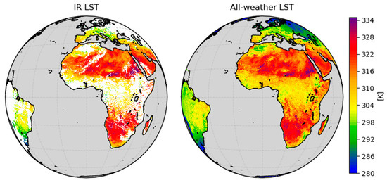
Figure 1.
Example the standard Satellite Application Facility on Land Surface Analysis (LSA-SAF) infrared (IR) land surface temperature (LST) product based on the Spinning Enhanced Visible and Infrared Imager on Meteosat Second Generation (MSG/SEVIRI) measurements (left), compared to the corresponding all-weather LST counterpart (right). Data from 29 Sep 2016 1100UTC.
2.1.1. Clear Sky
The standard IR-based LSA-SAF LST product is only generated for clear-sky pixels, as clouds are opaque to infrared radiation. There are several empirical algorithms to retrieve LST from remote sensing data described in the literature [14,67,68]. The operational LST produced by the LSA-SAF uses a generalized split-windows algorithm specifically tuned to MSG/SEVIRI [16,19,69]:
where TIR1 and TIR2 are the top-of-atmosphere brightness temperatures in the split-window channels (10.8 and 12.0µm for MSG/SEVIRI), ε and Δε are their surface emissivity average and difference, respectively; and Ai, Bi and C are model coefficients. These coefficients are determined a priori by class of viewing zenith angle (VZA) and total column water vapor (TCWV). ε is estimated with the vegetation cover method [51], where the effective emissivity for each pixel is calculated as an average between the vegetation and the bare soil emissivities ( and , respectively) weighted by the fraction of vegetation cover (FVC) within the pixel, also provided by the LSA-SAF:
Values of and are taken from pre-computed lookup tables, where these values, together with an estimation of their uncertainty, are available per land cover type and per channel. These were estimated through the convolution of spectral emissivities available from published libraries (e.g., [70]) and MSG/SEVIRI channel response functions, considering a set of natural and man-made materials that are most common within typical land-cover types. A full description of the methodology, and lookup tables may be found in [19,51,71]. It should be noted that Equation (2) can be extended easily to the case of mixed pixels with water (or snow) and vegetated (or bare ground) surfaces. However, given the limitations in the estimation of FVC in those cases, we consider a climatological FVC when snow is detected ( is set to a “snow” value), while all cases where more than half of the pixel is covered by coastal or inland water are treated as “pure” water pixels (FVC set to 0 and is set to a “water” value).
2.1.2. Cloudy Sky
For cloudy pixels, a surface EB model approach is used to derive surface temperature. In order to provide estimates of evapotranspiration, the surface energy balance is solved every 30 min using the LSA-SAF ET v2 algorithm (see respective Algorithm Theoretical Basis Document ATBD available from http://lsa-saf.eumetsat.int/). A brief description of this EB model is given below; a more complete description may be found in [57,72,73,74]. A schematic representation of the model is provided in Figure 2.
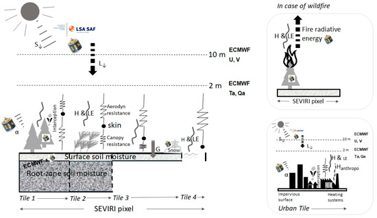
Figure 2.
LSA-SAF surface energy balance model. Over each tile the model is solved for a variety of inputs including downwelling radiative fluxes (, ), surface albedo (), vegetation properties (all from LSA-SAF), surface and root zone soil moisture (hydrology SAF) and near surface meteorological variables from ECMWF (, , and ). Separate schemes are used for wildfire and urban tiles. All quantities obtained from satellite have an MSG icon next to them. The related definitions are provided in the main text.
Each MSG/SEVIRI pixel is considered to be composed of homogeneous tiles corresponding to different surface types, e.g. bare soil, several classes of low and high vegetation, water, snow, rocks and urban surfaces. The surface energy balance is solved for each tile i separately:
where is net radiation, is sensible heat, is latent heat and is ground heat flux for the i-th tile of within a pixel. All these terms are parameterized as a function of several other variables and the reader is referred to the product ATBD for the specific details. The fraction of each tile within a MSG/SEVIRI pixel and its respective parameters are determined from the ECOCLIMAP-II database [75,76].
Net radiation () is determined for each tile from the shortwave and longwave fluxes at the surface:
where is (pixel) surface albedo, is (pixel) broad-band infrared emissivity, and are the (pixel) downward shortwave and longwave fluxes at the surface, respectively, is the Stefan–Boltzmann constant and is the skin temperature of the i-th tile. Skin temperature is also involved in the estimation of latent and sensible heat fluxes, which are obtained using a resistance approach, combining the effects of: (1) the stomatal aperture, modeled using the canopy resistance , conditioned by environmental stress, which in turn depends on factors such as the LAI, , unfrozen soil water content and atmospheric water pressure deficit, as well as plant physiological characteristics; and (2) the aerodynamic resistance , which depends on the stability of the atmosphere and turbulence intensity. Thus, sensible heat flux is given by:
where is air density, is the specific heat of dry air at constant pressure, and are skin and air temperatures (at tile and pixel level, respectively), is the acceleration of gravity and is the height at which air temperature is estimated (2 m). Latent heat flux is given by:
where is the latent heat of vaporization and and are the specific humidity and the specific humidity at saturation, respectively. Finally, the heat flux into the ground () is parameterized as a function of net radiation and LAI. Skin temperature and turbulent heat fluxes are adjusted iteratively to meet the surface energy balance, given the prescribed satellite and numerical weather prediction model inputs.
Land surface parameterization schemes similar to the one that is used here have been widely used to represent surface fluxes at various spatial and temporal scales in numerical prediction models (e.g., [62,63,64,65]). In contrast to these, the model is run at SEVIRI pixel scale exploiting as much as possible inputs derived from satellite observations, most of them retrieved by LSA-SAF from MSG/SEVIRI observations. These include incoming radiation at the surface, namely shortwave and longwave downward radiation fluxes [50,53,77,78], albedo [52], and vegetation related parameters such as the LAI [50].
For pixels with active fires, identified using LSA-SAF fire radiative power [60], the skin temperature is not estimated. A snow mask is also used (MSG/SEVIRI-based distributed by the Hydrology SAF, H-SAF; http://h-saf.eumetsat.int) for the identification of non-permanent snow pixels. The clear-sky 15-minute LST is itself used to help inferring the soil moisture content in arid in semi-arid regions, where the morning heating rate of the surface relates to soil moisture [5,79,80]. The information on soil moisture is further complemented with H -SAF soil moisture data (product identifier H14 SSM, also known as SM-DAS-2; [81]), based on observations made by the Advanced SCATterometer (ASCAT) on board Metop satellites. Near- surface meteorological fields such as 2 m air temperature and specific humidity, surface pressure and wind speed at 10 m are retrieved from the latest available ECMWF operational forecasts (up to 24 hours) and resampled to the MSG/SEVIRI grid. The ECMWF data are available hourly and the set of fields closest in time to SEVIRI observations is used. The forecasts (current operational model has a horizontal resolution of about 9 km) are bi-linearly interpolated to the SEVIRI geostationary projection; air temperature is further corrected using a constant lapse rate to account for differences between model and pixel topography.
The surface energy balance is solved under all-sky conditions and, therefore, skin temperature is also produced for all weather conditions. There are very few situations for which the model does not converge after a sufficiently large number of iterations (it stops after 100 iterations). In these cases, the model does not provide a valid skin temperature value. In all other cases (except for active fire pixels as stated above), EB model skin temperature is used to fill the cloudy pixels in the clear sky LST product.
2.2. Microwave-Based Advanced Microwave Scanning Radiometer-Earth Observing System (AMSR-E) LST
An alternative approach to obtain LST under all-sky conditions consists in the use of microwave observations, as these are nearly unaffected by clouds. MW LST data used here corresponds to the dataset developed by Jimenez et al. [25], where a neural-network approach is applied to brightness temperatures measured by the AMSR-E instrument on-board Aqua satellite at 18.7, 23.8, 36.5 and 89.0 GHz. The effective mean resolution of the product is 12 km (footprint size of the 36.5 GHz channel), but information from the channels with larger footprints also affects the retrieval. The AMSR-E LST is produced twice-daily for almost all weather conditions at equator crossing times of 1:30 AM/PM.
For this dataset, several limitations have been identified by Jimenez et al. [25]: (1) less reliable retrievals can occur in regions where the emissivity can depart from the assumed climatological value such as surfaces with very low emissivity, potentially flooded areas, snow/ice surfaces with changing conditions (e.g., melting), and coastal pixels; (2) the radiation reaching the sensor may include emissions from subsurface layers, specially over dry sandy areas; and (3) the ice phase of deep convective clouds may scatter microwave radiation.. The latter conditions are flagged by looking for cloud scattering signals in the 89 GHz channel.
Ermida et al. [26] performed comparisons of clear-sky LSTs for AMSR-E and MODIS and a few geostationary sensors. They found good agreement between MW and IR estimates, except in arid and semi-arid regions, where differences of up to 6–7 K were reported, and in snow covered areas, where LST differences may reach 20 K. The main advantage of the AMSR-E dataset compared to the MODIS counterpart is its much larger frequency of successful retrievals: the authors showed that for frequently cloudy pixels, the increase in coverage in AMSR-E compared to MODIS exceeds 250%.
Based on comparisons made against a training database used to calibrate the neural network algorithm, Jiménez et al. [25] reported an expected precision of 2.8 K or better for almost 75% of the global land surface. A comparison with in situ stations spread across a wide range of biomes and climates showed a RMSD of around 4 K, which is larger than that reported for MODIS (around 2.4 K), but with nearly 3 times more sampling due to its ability to measure LST even under cloudy conditions.
For the purpose of comparison with MSG/SEVIRI-based all-weather LST, we consider LST derived from AMSR-E [25] for the whole year of 2010.
2.3. In Situ LST
The LST estimates from the LSA-SAF MSG/SEVIRI (level-2) product are routinely validated against dedicated in situ stations, equipped with upward and downward looking longwave radiometers, the “KT15.85 IIP” produced by Heitronics GmbH, Wiesbaden, Germany. This type of instrument measures thermal infrared radiance in the 9.6 – 11.5 µm interval with a 0.03 °C resolution and ±0.3 °C accuracy over the corresponding temperature range. In this work, data from three permanent LST validation stations operated by Karlsruhe Institute of Technology (KIT) are used. These are located within the MSG/SEVIRI disk (Figure 3): Évora (Mediterranean, Portugal), Kalahari (Steppe, Namibia) and Gobabeb (Desert, Namibia). This study considers all data collected by stations dedicated to LST validation for this period over the MSG/SEVIRI disk. Due to the relatively large pixel size, stations need to be located in large homogeneous landscapes, where in situ “point-measurement” (e.g. covering an area of 10 m2) are representative of the about 25 km2 corresponding to the MSG/SEVIRI pixel scale.
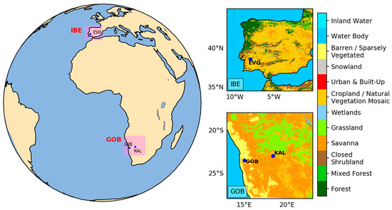
Figure 3.
Locations of the dedicated LST validation stations used in this study. The colors in the right-hand plots represent the land cover types from the International Geosphere-Biosphere Programme (IGBP) database [86].
The in situ LST (here referred to as ) is estimated from the measured upward radiance corrected for the downward radiation reflected by the surface and local surface emissivity [17,18,20,82]:
In (7), surface emissivity is either estimated from the corresponding value for the 10.8 µm MSG/SEVIRI channel, combining vegetation and bare ground emissivities of the land cover attributed to the pixel containing the station, or set to a constant value, e.g. at the Gobabeb desert site [83,84]. Surface temperature is then derived with the inverse Planck function, at the central wavelength of the radiometer response function (:
where , , and is the center wavelength of the downward looking radiometer.
Evora is located within an oak tree woodland, where temperature contrasts between tree canopies and the sunlit and shaded understory may be high, especially during the dry summer season. Such contrasts may lead to significant directional effects that should be taken into account when upscaling the in situ measurements to pixel scale [18,85]. Following Ermida et al. [18], Evora in situ LST is upscaled using a geometric model to simulate the satellite-viewed fractions of tree canopy and sunlit and shaded ground, taking into account the illumination and viewing geometries and a typical tree shape for the region. These fractions are then used in combination with the available measurements of tree canopy, sunlit ground and air temperatures (used as proxy for shaded ground temperature) to estimate the LST as would be retrieved by the satellite. However, it must be stressed that while MSG/SEVIRI IR LSTs are retrieved directly from the measured thermal emissions at a given viewing geometry, EB estimates correspond to an average of tile skin temperature, which assumes tile fractions based on the ECOCLIMAP-II database and disregards any shadowing effects. Therefore, the correction method developed by Ermida et al. [18] is only applied to the in situ clear sky values used for the validation of clear sky LST values retrieved via the split-windows algorithm. The validation of EB skin temperature makes use of in situ observations upscaled using known fractions of tree canopies/open ground around the station. Clear sky pixels over the station sites are identified using the MSG/SEVIRI cloud mask. For Gobabeb and Kalahari no such corrections are needed since there are very few surface elements casting shadows.
A summary of all the datasets used in this study is provided in Table 1.

Table 1.
Characteristics of the products used in this study. All datasets are available for the full year of 2010, except the energy balance (EB) model ; for the latter, full disk retrievals were performed for 10 days in January and 10 days in July; for the full year, retrievals every 30 min were performed for the pixels matched with the in situ stations.
2.4. Statistical Metrics
In this study, for the comparison with in situ data, we use robust statistics recommended by the Committee on Earth Observation Satellites Working Group (CEOS) on Calibration and Validation-Land Product Validation (LPV) Subgroup for validation of Land Surface Temperature Products [82,87]. The median error, , which is a measure of the accuracy is given by:
where stands for satellite LST and represents in situ LST. The median of the absolute residuals, , reports on precision and is given by:
Finally, an estimate of total uncertainty is given by root-mean-square-difference, RMSD:
where represents the sample size.
For the comparison of satellite datasets, the traditional average (bias) and standard deviation (STD) of LST differences are used instead of the robust metrics.
3. Results
3.1. Infrared (IR) and Energy Balance (EB) Model Comparison in Clear Sky Situations
Figure 4 shows a direct comparison between EB model skin temperature and IR LST (over clear sky scenes). Such comparisons for clear sky cases, while taking into account uncertainty in IR LST, are helpful in providing insights into model capabilities and weaknesses. This is important for future model improvements, in particular over areas where in situ observed data used for model calibration are scarce. The mean differences were computed using the full 10-day period processed for January and July 2010, respectively, but accounting only with cases where both EB skin temperature and IR LST are simultaneously available. Daytime and nighttime cases were analyzed separately, averaging half-hourly timeslots between 00:00UTC and 02:30UTC for nighttime and between 12:00UTC and 14:30UTC for daytime. In general, the results in Figure 4 are similar to those found in previous comparison studies between model skin temperature and satellite LST [10,11,88,89]. Namely, they show a tendency for model surface temperatures to have a lower daily amplitude, particularly over arid and semi-arid regions – see the strong negative daytime bias of −4 to −7 K over the Iberian Peninsula in July, of −2 K to −4 K over part/most of Northern Africa in July/January and of −1 K to −5 K in Southern Africa in January. The nighttime bias over the same areas/months suggests that model surface temperature stays warmer than IR LST, also in agreement with the aforementioned model comparisons, although the results presented here show a higher level of detail. Indeed, here we run an EB model at high spatial resolution (MSG/SEVIRI pixel scale) and force it with a combination of satellite and ECMWF data, which may contribute to the differences in the results. The information contained in Figure 4 is complemented by Figure 5, which shows the corresponding histograms of the instantaneous differences for the same period and area. Daytime differences show a positively skewed distribution, i.e. for January (July) 1.7% (6.3%) of the datapoints are above 10 K, while only 1.2% (0.9%) are below –10 K. The mode of both distributions (January and July) is −1.5 K (for 1 K histogram bins). Since the frequency of larger positive differences in July increases, the absolute median difference decreases from 1.2 K (negative) in January to 0.0 K in July. During nighttime, these larger differences are less frequent and the distributions are less skewed. For January (July) only 0.4% (0.9%) of the differences exceed 10 K, while 0.2% (0.1%) have values below –10 K. Furthermore, for January the negative bias is reduced ( = –0.3 K), while it is slightly positive ( = 0.6 K) for July.
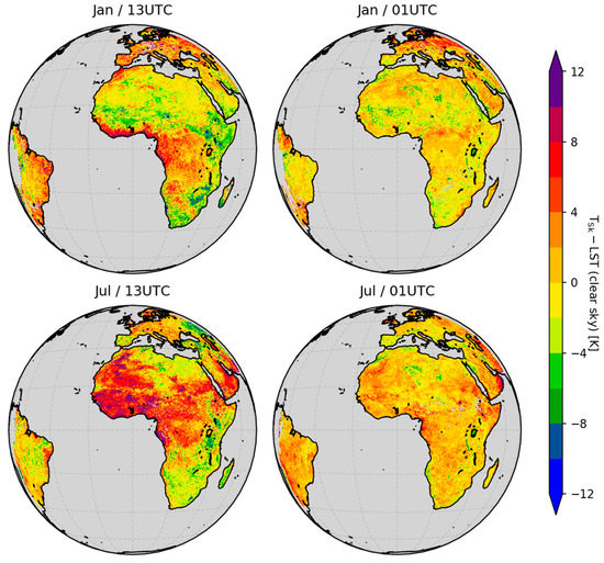
Figure 4.
Mean difference between EB model skin temperature () and IR LST (clear sky only), as minus LST. Data averaged over a 2 h 30 period around the time indicated in each plot, and averaged over 10 days for January and 10 days for July 2010.
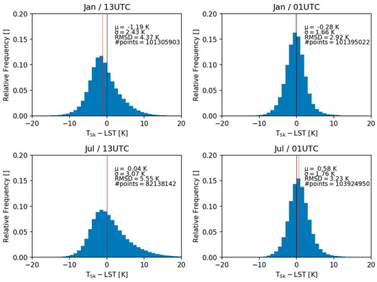
Figure 5.
Histograms of the instantaneous clear sky differences of in Figure 4 (units: K). The red dashed line denotes the median difference. Also indicated are the values of the median difference, , the median of the absolute residuals, , the root mean squared difference (RMSD) and the number of pixels used in the comparison.
Areas with frequent cloud cover (see e.g., the tropics, mid-latitudes winter) tend to exhibit a clear positive bias, which needs to be further investigated. Figure S1 shows the number of data points used to compute the median differences in Figure 4. Over some of the aforementioned regions (e.g., Central Africa in July, where the Intertropical Convergence Zone lies) the number of EB versus IR LST matchups decreases significantly, with large areas with less than 6 matchups. There, IR LST is more prone to cloud contamination, which may contribute to the observed positive bias.
Possible reasons for the observed discrepancies are discussed in Section 4. Note that clear-sky EB model skin temperature is not used in the proposed all-weather LST product. Comparisons were also performed using the full month of July of 2018 (since all the inputs were readily available for that period) and the obtained patterns are very similar to those shown in Figure 4 (not shown), with exception of a reduced positive bias over West Africa at 13UTC. This reduction could be related to the higher sampling available for the comparison. This confirms the systematic character of these biases and the need for further model improvements.
3.2. IR and EB Model In Situ Comparisons
3.2.1. Time Series
To illustrate the general behavior of the different products, Figure 6 provides time-series of the various LST datasets for Evora (in situ with and without directional correction, IR split-window LST, all-weather EB model and AMSR-E LST), for a spring (23 March–7 April 2010) and summer (7–22 August 2010) period. The area surrounding Evora station experiences strong seasonal (and inter-annual) vegetation variability as the understory grows and desiccates. This introduces some emissivity variability as well as significant temperature contrasts between surface elements, particularly during summer. A correction that accounts for directional effects was introduced in order to improve comparisons with MSG/SEVIRI level 2 clear-sky LST estimates [18,90]. The adjusted time series (shown in green) show differences to the original in situ estimate up to 2 K, with lower LST values around the daily maximum for the periods shown. This is plausible since the non-adjusted in situ values correspond to a composite of sunlit ground and tree canopy temperatures and do not include the fraction of shaded areas observed by MSG/SEVIRI.
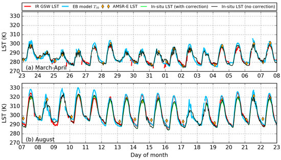
Figure 6.
LST products over Evora station: IR clear-sky LST (red line), EB model (all-weather) (blue line), in situ LST without directional correction (black line), in situ LST with directional correction to MSG/SEVIRI viewing angle (in green) and AMSR-E LST (yellow diamonds). Spring is characterized by mild temperatures and high soil moisture (top panel), and summer is characterized by warm temperatures and low soil moisture (bottom panel).
The IR LST follows the in situ curve quite closely, with some negative differences for partly cloudy days (these differences are quantified below). The EB model skin temperature seems to ‘overshoot’ at the daily maximum by a few degrees, whereas at nighttime it gets cooler than in situ observations for some days (e.g., 2–3 Apr, 12–13 Aug), and warmer for others (e.g., 9–10 Aug). Regarding the AMSR-E all-weather LST product, at nighttime in August there is a clear overestimation of in situ LSTs. At daytime these differences are reduced, i.e. AMSR-E LST does not show the overshooting behavior of EB model and of IR LST (see days 7, 13–16, 19–20 and 22 of August). Note that some days (e.g. 27 or 29 of March) do not show any AMSR-E values, which is due to the fact that the closest measurement was too far from the station (i.e. more than 12 km away). AMSR-E revisiting time is generally between 1 to 2 days.
In Figure 7 the EB model skin temperature (separated into clear sky and cloudy sky cases) is evaluated against in situ estimates for the 3 stations, as well as the IR LST (for clear sky only) and the derived all-weather LST product i.e., IR LST (clear sky) + EB (cloudy sky). The matchups are performed using the nearest neighbor of the station, except for Gobabeb, where a specific pixel in the vicinity of the station, the so-called Tidbit01 location, was used to avoid the effect of the sand dunes surrounding the station [17,20]. Each plot of Figure 7 contains the summary statistics described in Section 2.4, and global summary statistics are shown in Table 2. All datasets are sampled in 30 min frequency for the matchups. Colocations are only possible when all datasets are available. If any of the inputs for the IR LST and EB models are unavailable at the time of the processing, or are of low quality, all-weather LST cannot be obtained. In situ stations also contain missing data.
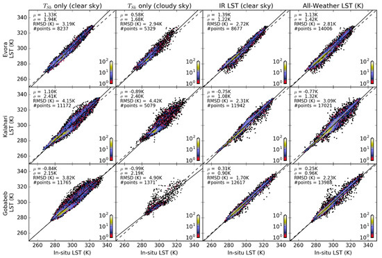
Figure 7.
Scatterplots comparing the various LST estimates and matched-up in situ LST. Left to right column: clear-sky EB model skin temperature, cloudy-sky EB model skin temperature, IR LST (clear-sky) and all-weather LST product (IR LST + Cloudy Sky EB model skin temperature). Top to bottom row: Evora, Kalahari, Gobabeb. Also shown are summary (robust) statistics: median difference (), median absolute deviation (), root-mean-square differences (RMSD), and number of matchups (#points). Colors denote data point density, computed over a 100 × 100 grid. Axes are common to all panels.
Table 2.
Overall average summary statistics (each in situ station was weighted by its number of available observations for each case), for the skin temperature (clear-sky and cloudy sky), for the IR LST and for the all-weather LST (IR LST for clear sky + EB Skin Temperature for cloudy sky).
The comparison of clear sky EB model and IR LST statistics complements the results shown in Figure 4, and shows that the IR LST outperforms the EB model for all stations, both in terms of accuracy, precision and uncertainty, supporting its use for clear sky cases in the all-weather LST product. The clear sky RMSD may be up to 2 K higher than that obtained for the IR LST, with larger differences for Kalahari and Gobabeb stations. Considering the cloudy cases, the estimated bias was found to range between –1.0 K and +0.6 K, close or below what was found for and IR LST clear sky cases, while the RMSD ranged between 2.9 and 4.9 K. The latter value was obtained for the desert site in Gobabeb, where the frequency of cloudy cases is the lowest (less than 13%). It should be noted that cloudy LST scatter plots of the desert stations show higher dispersion of the points for higher values of LST. This indicates that these observations are likely performed under broken clouds, which may lead to discrepancies between point measurements and the pixel scale estimates.
The all-weather product (IR split-window LST for clear sky + EB model skin temperature for cloudy cases, right column in Figure 7) shows statistics that are well within the acceptable range for LST products (see overall statistics in Table 2), with a mean accuracy of 0.1 K, precision of 1.2 K, and a RMSD of 2.7 K. These values are only slightly worse than the standard IR LST retrieval (whose statistics for 2010 are: 0.2 K accuracy, 1.1 K precision and 2.2 K uncertainty). For Evora and Kalahari stations, the new all-weather product increases the number of available samples by around 60% compared to IR LST.
3.2.2. Median Diurnal Cycle of Error
Figure 8 shows the diurnal cycle of the median of the differences between the IR LST and the EB model skin temperature and the corresponding in situ, for each station and season (December, January and February—DJF; March, April and May—MAM; June, July and August—JJA; September, October and November—SON). The IR LST itself shows a somewhat pronounced error in diurnal cycle, reaching generally lower values (often negative) at nighttime and larger (positive) during daytime, when spatial heterogeneity becomes larger and directional effects become non-negligible. For example, in MAM over Kalahari, satellite IR LST overestimates in situ LST by about 3.5 K at daytime and underestimates it at nighttime by about 1.2 K. The clear sky component of the EB model, shows a somewhat similar behavior, but with larger amplitudes and, in some cases, with large phase differences (i.e. its maximum is reached earlier in the diurnal cycle, when compared to other estimates). This is more pronounced for Kalahari and Gobabeb stations. For Kalahari in DJF the model overestimates in situ surface temperature by about 6 K in the early morning, whereas for IR LST the largest differences are found around noon. This is consistent with the larger dynamic LST range at that time of day. Over these three stations, the results suggest that the model struggles to reproduce in situ surface temperature for drier seasons/locations, e.g. for Evora in Winter (DJF) the differences are smaller than in Summer (JJA), when the landscape surrounding the station is much drier.
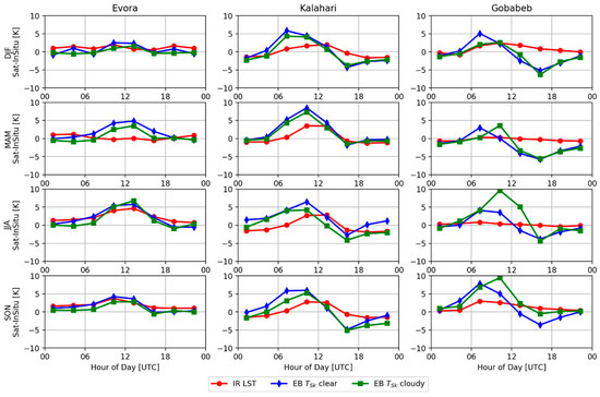
Figure 8.
Diurnal cycle of the median differences between satellite and in situ surface temperature estimates (K) for each station and season (December, January and February—DJF, April and May—MAM, June, July and August—JJA and September, October and November—SON). IR LST is represented in red, and the clear (cloudy) sky cases of EB skin temperature are represented in blue (green). Values were averaged over 3h. Axes is common to all panels.
Regarding the cloudy sky (EB model) , the signal is somewhat different in Kalahari and Gobabeb, suggesting that it is caused by different factors, including the diurnal sampling of cloudy conditions (e.g., Gobabeb has frequent morning fog but almost no clouds in the afternoon). The bias usually changes sign in the late afternoon, with almost all cases showing a more or less negative median difference. These may be partly explained by the occasional presence of opaque convective clouds, which directly affect the inputs of the EB model such as the shortwave and longwave surface radiative fluxes. During the early morning, the model generally overestimates the in situ values by a few degrees. These comparisons are currently being used to tune the EB model in terms of its internal parameterizations, in order to improve the representation of the amplitude and the phase of the signal, which could lead to improvements of other variables obtained from the EB model (such as surface turbulent fluxes).
3.3. Comparison to AMSR-E
3.3.1. In Situ Comparisons
The full year of 2010 LST retrievals from AMSR-E LST was compared with both the IR LST + EB model All-Weather LST product and with in situ LST data from the aforementioned stations. The AMSR-E estimates used here were already validated against in situ [25] and independent measurements over clear sky pixels [26]. The purpose of this section is to assess the quality of the new all-weather LST product by comparing it to the performance of an alternative product.
Data from the 3 sources were carefully collocated in order to ensure similar sampling between MSG/in situ and AMSR-E/in situ comparisons. For all AMSR-E swaths in 2010, the closest pixel to the station was determined and only considered if its distance was less than 5 km. Then the in situ value closest in time (i.e. 30 s or less apart) was determined. To ensure similar sampling, the closest MSG/SEVIRI-based all-weather LST value (i.e. at most 7.5 min and 5 km apart) is determined and collocated to its in situ counterpart in the same way. If any of the collocated values are invalid, then all of them are disregarded. This way, the same sampling in the comparisons is ensured, with similar MSG/SEVIRI and AMSR-E observation conditions.
Figure 9 shows both all-weather LST products plotted against the corresponding in situ LST from each station. Due to the much lower number of AMSR-E observations, the number of matchups is much smaller than in Section 3.2. The scatterplots were separated into clear/cloudy and day/night cases and the results are summarized in Table 3. The EB+IR-based product presents accuracies between –0.4 and +1.5 K, while the corresponding values for the MW LST lie between –4.4 and +1.1 K. The MW LST accuracy index is largest at Gobabeb (indicating larger differences to in situ), presenting negative values for both day and night-time. Although the reasons for the poorer comparison over Gobabeb for all cases in Figure 9 are still unclear, it may be due to 1) contamination of the retrieval by the nearby sand dunes, particularly considering the spatially coarser AMSR-E pixels; 2) the sensitivity of the MW signal to the subsurface, particularly in dry soils, while the in situ LST represents skin temperatures [41]. For Kalahari, the median error of the IR+EB LST is relatively low, but when results are separated into day and night retrievals, they show a positive bias of around 3.5 K at daytime and a negative bias of –1.5 K (–2.5 K) for clear-sky (cloudy) cases. It must be taken into account that Aqua’s afternoon overpass time corresponds to the time of day at which the errors are higher (see Figure 8). The values of the AMSR-E estimates are less precise than the MSG/SEVIRI-based all-weather LST, most likely due to the larger AMSR-E pixel size, which makes the in situ value less representative of the satellite observations. The RMSDs are comparable for Evora, but for Kalahari and Gobabeb the AMSR-E RMSD increases by about 0.8 K and 3.0 K with respect to MSG/SEVIRI estimates.
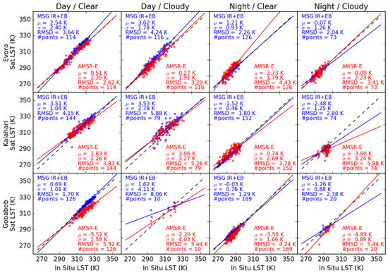
Figure 9.
Energy balance (EB) + infrared (IR) based all-weather LST (blue) and microwave (MW)-based all-weather LST (red) against in situ LST estimates, for Aqua satellite overpasses at the three stations (rows). Axes are common to all panels.
Table 3.
Summary statistics for the point comparisons of the MSG/SEVIRI IR+EB and AMSR-E products with collocated in situ estimates from 3 stations.
3.3.2. Spatial Comparisons
In order to provide a more thorough evaluation of the new product against independent all-weather LST estimates, AMSR-E retrievals for the days mentioned in Section 2.1 (i.e. 10 days in January and 10 days in July 2010) were collocated with MSG/SEVIRI over a 0.15° regular grid, which is approximately the resolution of AMSR-E retrievals. Lower quality estimates of the AMSR-E LST product (described in Section 2.2) were identified using its quality flags and then removed. Again, the closest MSG/SEVIRI retrieval in time was used (if available), with time differences of up to 7.5 minutes.
Figure 10 shows the median differences (calculated over January 2010 in the top row, and July in the bottom row) between MSG/SEVIRI-based and AMSR-E based all-weather LST products. The retrievals were further separated into day and night-times and cloudy and clear-sky. The central part of Africa is widely covered by clouds and shows an area of positive differences (i.e. MSG/SEVIRI warmer than AMSR-E), which is more pronounced in daytime; this area moves northward following the mean location of the ITCZ in July. In the July cloudy case, the southern Sahel shows a high positive median difference that stands out during nighttime, which may be related to unusually cold AMSR-E LST from convective cloud contamination or wet soils due to rain events or flooding, which would lower emissivity. This effect may actually affect MW estimates everywhere, when soil moistening due to rain or flooding happens. Over desert areas, median differences are generally negative, with some smaller areas of positive differences. At daytime, any biases due to MW sub-surface emission are likely to be positive, i.e., AMSR-E LST being colder because emission originates from typically colder sub-surface layers, so other factors should be responsible for the observed differences. The uncertainty of MSG/SEVIRI based LST also tends to be higher in those regions, mainly because under dry atmospheres the sensitivity of the IR LST retrieval algorithm to uncertainty in surface emissivity is large (e.g., [19]). These results are in general agreement with the clear sky-only comparisons of Ermida et al. [26].
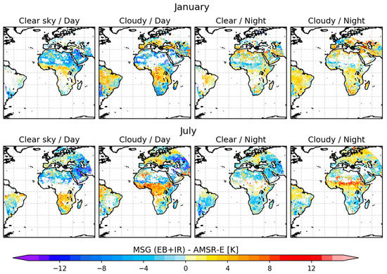
Figure 10.
Median differences between MSG/SEVIRI and AMSR-E based LST estimates for (left) daytime clear sky (center-left) daytime cloudy (center-right) nighttime clear sky (right) night-time cloudy. All AMSR-E quality flags were applied. Data from January 2010 (top row) and July 2010 (bottom row). Missing values are shown in white.
Table 4 summarizes the statistics of these comparisons, separated into clear and cloudy cases, day and night, for January and July. The clear and cloudy statistics are comparable especially in terms of RMSD (smaller during nighttime). The bias is generally negative in the clear sky cases (except in January, night-time case). Moreover, it is larger during daytime for the clear sky cases; and larger in the nighttime for cloudy cases, which could be due to lower reliability of the cloud mask as visible channels are not available.
Table 4.
Summary statistics for the MSG/SEVIRI AMSR-E all-weather LST differences, for clear sky versus cloudy sky pixels, separated into day and night retrievals, for the whole MSG/SEVIRI disk. All AMSR-E quality flags were applied. Data from January 2010 (top) and July 2010 (bottom).
In Figure 11 the MSG/SEVIRI–AMSR-E differences are analyzed by land-cover type, for January and July, separated into day/nighttime and for clear/cloudy conditions. Land-cover types from the IGBP database [86] were aggregated into more general classes to simplify the analysis (forest, mixed forest, closed shrub lands, savannas, grass lands, permanent wetlands, croplands and newly vegetated areas, urban, snow and ice, barren, open water and inland water). This dataset was re-projected to the regular grid used to perform the comparisons and the most frequent land cover class for each grid point is considered. Due to re-gridding and land cover class aggregation, some differences between the land cover used in the processing of each dataset may be present.
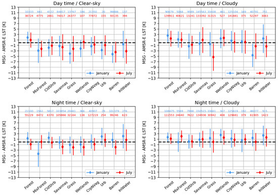
Figure 11.
Comparison between MSG/SEVIRI-based and AMSR-E all-weather LST products by land-cover type. The top row shows the values for daytime and the bottom values for nighttime. Results for clear sky (left columns) and cloudy pixels (right column). Blue indicates for January and red the corresponding values for July; whiskers represents , and numbers indicate the available matchups.
For clear-sky pixels, the daytime bias is negative for all land cover classes (in January and July), except forests and wetlands (in July). Classes with significant seasonal variability of vegetation (e.g. grasslands) show larger differences in the statistics between January and July, possibly due to differences in how surface emissivity is taken into account in the retrieval algorithms. However, other factors may play a role, namely a larger spatial heterogeneity often experienced by those land-cover types (e.g., closed shrubs, grass) during the dry season, which may increase directional effects and lower representativeness. Standard deviations are in general larger for the July case, except for mixed forest. Different seasons may be mixed up within each land class/month, as contributing pixels may originate from very different geographic areas within the MSG/SEVIRI disk. For the cloudy case, daytime biases are generally smaller in magnitude and show positive and negative signals depending on land cover class and month. Over grasslands and barren soils, there are very large differences between the two periods. This could be an artifact produced by poor detection of deep convection by AMSR-E and/or by MSG/SEVIRI. The majority of those pixels is located over or south of the Sahel, which experiences a pronounced seasonal cycle affecting both surface and atmospheric conditions. Under the influence of the ITCZ (July in this area) there are frequent deep convective clouds, not always properly flagged, which produce large amounts of precipitation. These in turn may also affect surface emissivity, particularly in the case of the MW product. Large areas of positive bias are also found north of the Caspian and Black seas (cf. Figure 10), at the edge of the MSG/SEVIRI disk, particularly for cloudy cases. These regions are also characterized by frequent continental convection, especially in the afternoon.
The night-time bias for clear sky cases shows some dependence on season, although in general MSG/SEVIRI is colder than AMSR-E. The standard deviations are somewhat smaller than those for the daytime case, as expected. The night-time cloudy cases show a different picture, with IR+EB model LST being warmer than AMSR-E for all land covers.
4. Discussion
The proposed all-weather LST, based primarily on MSG/SEVIRI observations, represents a considerable leap forward, since it overcomes one of the main limitations of IR products, namely missing LST for cloudy scenes. One of its advantages is that any remote-sensing imager capable of providing the inputs to the EB model as well as the IR LST estimates for clear sky sky is suitable for the proposed product. This is the case for most imagers on current geostationary satellites (e.g. the Geostationary Operational Environmental Satellite (GOES)-R operated by the National Oceanic and Atmospheric Administration (NOAA), Himawari operated by the Japan Meteorological Agency, or MSG/SEVIRI Indian Ocean Coverage, operated by the European Organisation for the Exploitation of Meteorological Satellites – EUMETSAT) and polar orbiters (e.g. the Visible Infrared Imaging Radiometer Suite – VIIRS – operated by National Aeronautics and Space Administration (NASA)/NOAA, MODIS operated by NASA, MetOp operated by EUMETSAT, Sentinel-3 operated by the European Space Agency).
For clear skies, a standard retrieval methodology for IR sensors with two adjacent channels in the split-window region of the electromagnetic spectrum is used. Since this is a well-established method, its performance and limitations are well known and documented in the literature [17,19,69,91,92]. Figure 6 and Figure 7 show that this methodology usually performs well in clear sky situations. Furthermore, IR LST provides a better representation of the diurnal cycle in terms of its amplitude and phase.
Although the LST retrieval in cloudy sky cases uses a diagnostic model of the surface energy balance, the main forcing is provided by products generated from observations of the same sensor (MSG/SEVIRI), which constrain the physical model to produce more realistic LST estimates than schemes forced with inputs from an atmospheric model. The comparison of the EB model skin temperature with IR LST for clear sky cases (Figure 4) revealed some of the caveats that one might expect from such products. Apart from differences in cloud classification in the two datasets (discussed below), high aerosol loads (which are generally not well-accounted for) may also introduce errors into IR LST, and also into estimates of short-wave (and to a lesser extent long-wave) incoming radiation. It is known that aerosol loads are often underestimated (e.g., [93]), as is the case over northwest Africa in July (lower left panel in Figure 4). This explains the high positive bias at daytime: the underestimation of aerosol loads may actually lead to an underestimation of IR LST (attenuation of IR radiances not properly accounted for) and to an over-estimation of skin temperature (essentially due to overestimating solar radiation).
There are many other factors that may explain differences between clear sky EB LST and IR LST, ranging from model parameters (e.g., land cover, associated emissivity and roughness values) and model inputs (both ECMWF and satellite) to algorithm differences. Relatively large diurnal cycles of EB LST over inland waters (see positive/negative daytime/night-time bias over Lakes Victoria or Malawi, in Figure 4), which could be due to a too simplistic representation of lakes, e.g. by not considering mixing within a lake’s upper layers [94]. The relative simplicity of IR LST retrieval compared to EB LST estimation also allows a better understanding of error sources and their propagation to LST values. All these factors sustain the option to use a combination of IR LST and the EB model skin temperature to generate an all-weather LST by the LSA-SAF.
The validation of the EB skin temperatures estimated under cloudy conditions with in situ observations yielded somewhat better summary statistics than for clear-sky conditions, except for Gobabeb, which has significantly fewer clouds than Kalahari or Evora. Furthermore, when IR-based LST and EB are blended into an all-weather LST, the RMSDs against in situ data range between 2.2 and 3.1 K, which corresponds to an increase of 0.1 to 0.8 K compared to the RMSD of the clear sky IR LST. It is worth noting that the accuracy (bias) of the two LST products is considerably better than 2 K for clear skies as well as for cloudy skies. Moreover, the RMSD is only slightly above 2.5 K, the threshold value of the Climate Monitoring-SAF LST climate data record [95]. Guillevic et al. [82] proposed tighter thresholds of 1 K for both precision and uncertainty for an LST product to be useful for climate applications. However, existing LST products rarely achieve this target accuracy and it is also difficult to identify reference measurements with equally low uncertainties (e.g., [17,92]). The RMSD value of the proposed method (2.7 K) is slightly higher than that of the IR LST equivalent (2.2 K), therefore still being useful for a variety of weather and climate applications.
The comparison with in situ LST from 3 validation stations showed that the EB model skin temperature presents larger errors during mid-day, sometimes with a change of sign, particularly for the two African stations (Figure 8). The exact reasons still need to be identified, and will help to improve the model. Furthermore, factors such as precipitation, cloud type and amount also complicate the retrieval of the model inputs, thereby increasing their uncertainty. Problems in the representation of surface parameters in numerical models have already been acknowledged in the literature [9,10].
Downward short- and long-wave radiative fluxes may be estimated from satellite observations, mainly through their cloud signatures. Within the LSA-SAF, these are estimated every 30-minutes from MSG/SEVIRI measurements on a pixel-by-pixel basis. The respective algorithms described in Geiger et al. [53] and in Trigo et al. [50] make use of bulk parameterization schemes combined with information on cloud cover and type. When validated against 6 in situ stations spread across the MSG disk, the biases of LSA-SAF Downwelling Surface Shortwave and Longwave Flux products mostly within the target accuracy of 10% [50,53,77]. Furthermore, the two fluxes form a consistent dataset derived from the same source data, where errors in cloud amount and type tend to partially compensate each other [50,77].
One of the main (and harder to account for) sources of uncertainty in any LST retrieval is the presence of undetected clouds [96], which usually introduce negative biases into IR LST products. If the cloud mask algorithm fails to detect a cloudy or partly cloudy pixel, the cloud top temperature instead of the surface temperature is measured (or a mix of the two), which then causes the observed negative biases. This is likely to happen near cloud edges or under broken cloud, which may explain some of the large positive median differences observed for clear-sky LST in Figure 4, since these occur over areas where sampling is reduced due to increased cloud coverage. Comparing Figure 4 and Figure S1, this seems to be the case for Europe and South-Central Africa in January and for Central Africa, Eastern Brazil and Central Europe in July. Cloud contaminated pixels may affect spatial aggregation, e.g. when upscaling MSG/SEVIRI all-weather LST and AMSR-E LST to a common grid. Over partly cloudy areas this can, therefore, increase the bias between two satellite products. Cloud contamination can also affect comparisons between satellite and in situ data, since it impacts the representativeness of radiometric in situ measurements at the satellite pixel scale and, therefore, increases the dispersion in scatterplots. In the EB model, under overcast situations, thermal balance should be more easily reached, and directional effects are less important [97]. The simulation of clouds in numerical models, particularly those overlapping in time and space with those identified at satellite pixel scale is challenging. The impact of differences in cloud classification on mismatches between ECMWF model screen variables and MSG/SEVIRI radiation fluxes, as well as their impact on the estimation of turbulent fluxes and skin temperature, is not yet well known. However, the errors in the downward short- and long-wave fluxes tend to partially compensate for each other. Nevertheless, it should be noted that comparisons over areas where cloud frequency is high (e.g. as in Figure 4) are less robust, since the number of (clear sky) matchups is necessarily much lower. Overall, the errors due to cloudy sky situations are acceptable especially considering the increase in the number of available satellite LST data.
The validation of land surface products is usually performed against in situ estimates and against alternative estimates of the same variable retrieved from other sensors, mainly for consistency verification. Therefore, we used LST derived from AMSR-E as an alternative remote-sensing all-weather product to illustrate the regimes under which the retrieval is less certain and to assess the consistency between the two products derived with very different methodologies/observations. This is particularly interesting since the AMSR-E LST product is also quite recent. Although it was already compared against in situ [25], and IR LST from other sensors [26], the comparison of AMSR-E LST with the EB model LST extends the previous comparison to cloudy sky cases over large geographical areas. As described in [25], MW LST has its own issues, which need to be accounted for in any comparison with IR skin temperature. The quality of the AMSR-E product may be affected by situations that lead to variations of surface emissivities in the MW window, namely flooded surfaces and moist regions such as permanent wetlands, snow and ice or coastal areas, as well as by MW penetration depth. The expected deep convection impact on the MW retrievals was also noticed in this study. Failure to detect such situations impacted some of the comparisons, but it was also useful to discuss possible retrieval deficiencies in both AMSR-E and all-weather LST products. A more elaborate MW scheme to detect cloudy situations [98] is currently under development. Another factor to take into account is the 12 km resolution of AMSR-E, which is considerably coarser than MSG/SEVIRI resolution (3 km at nadir). This complicates comparisons with in situ LST even further, since over heterogeneous surfaces such point values become less representative with increasing pixel scale. One important advantage of the new IR + EB all-weather LST over existing MW products is its ability to finely sample the diurnal LST cycles.
5. Conclusions
Combining IR LST retrievals with skin temperatures obtained from an EB model yielded very promising results, particularly when compared to in situ LST obtained under all-sky conditions at three dedicated LST validation stations operated by the Karlsruhe Institute of Technology (Gobabeb and Kalahari stations, both in Namibia, and Evora, Portugal). The comparison of LST retrieved with the proposed method against in situ LST showed an overall accuracy between –0.8 K and 1.1 K, a precision between 1.0 K and 1.4 K and total uncertainty between 2.2. and 3.1 K, with some variations between stations associated with their representativeness on the satellite pixel scale. These statistics are within the range that is generally accepted for satellite IR LST products. In certain locations, the land surface model does not represent the LST diurnal cycle well (overestimation in the late morning and under-estimation in the late-afternoon/early-night in the dry season, particularly over areas with high seasonal vegetation variability). This behavior is currently under investigation and can hopefully be mitigated in future product versions.
The comparison of the IR+EB model all-weather LST and the AMSR-E LST against in situ LST showed that the former generally provides more accurate and precise LST estimates; an exception was station Evora, where AMSR-E showed a better accuracy (1.1 K for AMSR-E vs. 1.5 K for the IR + EB model product). To some extent this was expected, since AMSR-E has a considerably larger footprint than SEVIRI, and AMSR-E LST retrieval is physically more constrained. Compared to the AMSR-E product, the IR + EB model product provides a more detailed sampling of the diurnal LST cycle (since AMSR-E is onboard a polar orbiter). Spatial comparisons between both products showed that over moister areas, e.g. within the ITCZ, all-weather IR+EB model LSTs are generally warmer than AMSR-E LSTs, while over arid or semi-arid areas they are generally colder.
While the uncertainty budgets of IR-based LST have already been well studied in detail (see [19] for LSA-SAF standard LST product), such an exercise is still needed for the EB LST approach. The nature of the EB model and its larger variety of input data increase the complexity of error propagation for cloudy-sky LST estimates. However, such an exercise will help our understanding of the results presented here and will allow us to study the main sources of uncertainties in more detail and to identify aspects of the EB LST that can be improved. The main sources of uncertainty identified in this study are: cloud detection, the characterization of surface emissivity (mainly for IR retrieval), soil moisture information and surface net radiation (for the EB model). High aerosol loads affect both IR LST retrievals and various EB model inputs.
Finally, it should be stressed that the overall methodology is applicable to any remote-sensing imager capable of providing the inputs to the EB model as well as the IR LST estimates for clear sky situations. Thus, the presented method has the potential to provide a global, (nearly) gap-free all-weather LST product.
Supplementary Materials
The following are available online at https://www.mdpi.com/2072-4292/11/24/3044/s1, Figure S1: Number of data points used for the mean difference calculation, for each panel in Figure 4. White pixels denote no valid data points.
Author Contributions
J.P.A.M., I.F.T., N.G., F.G.-M. and A.A. developed the concept of the all-weather LST presented here and organized the results for the paper. J.P.A.M. wrote the first draft. C.J. and S.L.E. prepared the all-weather LST based on micro-wave observations. The in situ observations were obtained and up-scaled by F.-M.G., F.-S.O. and S.L.E. All authors contributed to the discussion of the results and final version of the article.
Funding
This work was performed within the framework of the LSA SAF (http://lsa-saf-eumetsat.int) project, funded by EUMETSAT.
Acknowledgments
The MSG/SEVIRI IR and EB model LST data were generated by the LSA SAF. The work at RMI has been funded by EUMETSAT and the European Space Agency through the PRODEX programme of the Belgian Science Policy. The AMSR-E/Aqua LST data was obtained through the GlobTemperature portal (http://data.globtemperature.info/). CJ acknowledges support from the European Space Agency (ESA) Data User Element (DUE) GlobTemperature project.
Conflicts of Interest
The authors declare no conflict of interest.
References
- Norman, J.M.; Becker, F. Terminology in thermal infrared remote sensing of natural surfaces. Agric. For. Meteorol. 1995, 77, 153–166. [Google Scholar] [CrossRef]
- Lakshmi, V. A simple surface temperature assimilation scheme for use in land surface models. Water Resour. Res. 2000, 36, 3687–3700. [Google Scholar] [CrossRef]
- Schmugge, T.J.; Becker, F. Remote Sensing Observations for the Monitoring of Land-Surface Fluxes and Water Budgets. In Land Surface Evaporation; Schmugge, T.J., André, J.C., Eds.; Springer: New York, NY, USA, 1991; pp. 337–347. ISBN 978-1-4612-3032-8. [Google Scholar]
- Caparrini, F.; Castelli, F.; Entekhabi, D. Variational estimation of soil and vegetation turbulent transfer and heat flux parameters from sequences of multisensor imagery. Water Resour. Res. 2004, 40, 1–15. [Google Scholar] [CrossRef]
- Ghilain, N.; Arboleda, A.; Batelaan, O.; Ardö, J.; Trigo, I.; Barrios, J.-M.; Gellens-Meulenberghs, F. A New Retrieval Algorithm for Soil Moisture Index from Thermal Infrared Sensor On-Board Geostationary Satellites over Europe and Africa and Its Validation. Remote Sens. 2019, 11, 1968. [Google Scholar] [CrossRef]
- Freitas, S.C.; Trigo, I.F.; Macedo, J.; Barroso, C.; Silva, R.; Perdigão, R. Land surface temperature from multiple geostationary satellites. Int. J. Remote Sens. 2013, 34, 3051–3068. [Google Scholar] [CrossRef]
- Bojinski, S.; Verstraete, M.; Peterson, T.C.; Richter, C.; Simmons, A.; Zemp, M. The concept of essential climate variables in support of climate research, applications, and policy. Bull. Am. Meteorol. Soc. 2014, 95, 1431–1443. [Google Scholar] [CrossRef]
- Good, E.J. An in situ-based analysis of the relationship between land surface “skin” and screen-level air temperatures. J. Geophys. Res. 2016, 121, 8801–8819. [Google Scholar] [CrossRef]
- Orth, R.; Dutra, E.; Trigo, I.F.; Balsamo, G. Advancing land surface model development with satellite-based Earth observations. Hydrol. Earth Syst. Sci. 2017, 21, 2483–2495. [Google Scholar] [CrossRef]
- Trigo, I.F.; Boussetta, S.; Viterbo, P.; Balsamo, G.; Beljaars, A.; Sandu, I. Comparison of model land skin temperature with remotely sensed estimates and assessment of surface-atmosphere coupling. J. Geophys. Res. Atmos. 2015, 120, 12096–12111. [Google Scholar] [CrossRef]
- Johannsen, F.; Ermida, S.; Martins, J.P.A.; Trigo, I.F.; Nogueira, M.; Dutra, E. Cold Bias of ERA5 Summertime Daily Maximum Land Surface Temperature over Iberian Peninsula. Remote Sens. 2019, 11, 2570. [Google Scholar] [CrossRef]
- Wang, A.; Barlage, M.; Zeng, X.; Draper, C.S. Comparison of land skin temperature from a land model, remote sensing, and in situ measurement. J. Geophys. Res. Atmos. 2014, 119, 3093–3106. [Google Scholar] [CrossRef]
- Trigo, I.F.; Viterbo, P. Clear-Sky Window Channel Radiances: A Comparison between Observations and the ECMWF Model. J. Appl. Meteorol. 2003, 42, 1463–1479. [Google Scholar] [CrossRef]
- Li, Z.-L.; Tang, B.-H.; Wu, H.; Ren, H.; Yan, G.; Wan, Z.; Trigo, I.F.; Sobrino, J.A. Satellite-derived land surface temperature: Current status and perspectives. Remote Sens. Environ. 2013, 131, 14–37. [Google Scholar] [CrossRef]
- Trigo, I.F.; Monteiro, I.T.; Olesen, F.; Kabsch, E. An assessment of remotely sensed land surface temperature. J. Geophys. Res. 2008, 113, 1–12. [Google Scholar] [CrossRef]
- Wan, Z.; Dozier, J. A Generalized Split-Window Algorithm for Retrieving Land-Surface Temperature from Space. IEEE Trans. Geosci. Remote Sens. 1996, 34, 892–905. [Google Scholar]
- Göttsche, F.M.; Olesen, F.S.; Trigo, I.F.; Bork-Unkelbach, A.; Martin, M.A. Long term validation of land surface temperature retrieved from MSG/SEVIRI with continuous in-situ measurements in Africa. Remote Sens. 2016, 8, 410. [Google Scholar] [CrossRef]
- Ermida, S.L.; Trigo, I.F.; DaCamara, C.C.; Göttsche, F.M.; Olesen, F.S.; Hulley, G. Validation of remotely sensed surface temperature over an oak woodland landscape-The problem of viewing and illumination geometries. Remote Sens. Environ. 2014, 148, 16–27. [Google Scholar] [CrossRef]
- Freitas, S.C.; Trigo, I.F.; Bioucas-dias, J.M.; Göttsche, F. Quantifying the Uncertainty of Land Surface Temperature Retrievals from SEVIRI/Meteosat. IEEE Trans. Geosci. Remote Sens. 2009, 48, 523–534. [Google Scholar] [CrossRef]
- Göttsche, F.M.; Olesen, F.S.; Bork-Unkelbach, A. Validation of land surface temperature derived from MSG/SEVIRI with in situ measurements at Gobabeb, Namibia. Int. J. Remote Sens. 2013, 34, 3069–3083. [Google Scholar] [CrossRef]
- Duan, S.B.; Li, Z.L.; Leng, P. A framework for the retrieval of all-weather land surface temperature at a high spatial resolution from polar-orbiting thermal infrared and passive microwave data. Remote Sens. Environ. 2017. [Google Scholar] [CrossRef]
- Crosson, W.L.; Al-Hamdan, M.Z.; Hemmings, S.N.J.; Wade, G.M. A daily merged MODIS Aqua-Terra land surface temperature data set for the conterminous United States. Remote Sens. Environ. 2012. [Google Scholar] [CrossRef]
- Zhang, X.; Wang, C.; Zhao, H.; Lu, Z. Retrievals of all-weather daytime land surface temperature from FengYun-2D data. Opt. Express 2017, 25, 27210. [Google Scholar] [CrossRef] [PubMed]
- Ermida, S.L.; Trigo, I.F.; DaCamara, C.C.; Jiménez, C.; Prigent, C. Quantifying the Clear-Sky Bias of Satellite Land Surface Temperature Using Microwave-Based Estimates. J. Geophys. Res. Atmos. 2019, 124, 844–857. [Google Scholar] [CrossRef]
- Jimenez, C.; Prigent, C.; Ermida, S.L.; Moncet, J.-L. Inversion of AMSR-E observations for land surface temperature estimation: 1. Methodology and evaluation with station temperature. J. Geophys. Res. Atmos. 2017, 122, 3330–3347. [Google Scholar] [CrossRef]
- Ermida, S.L.; Jimenez, C.; Prigent, C.; Trigo, I.F.; Dacamara, C.C. Inversion of AMSR-E observations for land surface temperature estimation: 2. Global comparison with infrared satellite temperature. J. Geophys. Res. Atmos. 2017, 122, 3348–3360. [Google Scholar] [CrossRef]
- Gao, H.; Fu, R.; Dickinson, R.E.; Juárez, R.I.N. A practical method for retrieving land surface temperature from AMSR-E over the amazon forest. IEEE Trans. Geosci. Remote Sens. 2008. [Google Scholar] [CrossRef]
- Holmes, T.R.H.; De Jeu, R.A.M.; Owe, M.; Dolman, A.J. Land surface temperature from Ka band (37 GHz) passive microwave observations. J. Geophys. Res. Atmos. 2009, 114. [Google Scholar] [CrossRef]
- Jang, K.; Kang, S.; Kimball, J.S.; Hong, S.Y. Retrievals of all-weather daily air temperature using MODIS and AMSR-E data. Remote Sens. 2014. [Google Scholar] [CrossRef]
- Zhao, E.; Gao, C.; Jiang, X.; Liu, Z. Land surface temperature retrieval from AMSR-E passive microwave data. Opt. Express 2017, 25, A940–A952. [Google Scholar] [CrossRef]
- Njoku, E.G.; Li, L. Retrieval of land surface parameters using passive microwave measurements at 6–18 GHz. IEEE Trans. Geosci. Remote Sens. 1999. [Google Scholar] [CrossRef]
- Aires, F.; Prigent, C.; Rossow, W.B.; Rothstein, M. A new neural network approach including first guess for retrieval of atmospheric water vapor, cloud liquid water path, surface temperature, and emissivities over land from satellite microwave observations. J. Geophys. Res. Atmos. 2001, 106, 14887–14907. [Google Scholar] [CrossRef]
- Basist, A.; Grody, N.C.; Peterson, T.C.; Williams, C.N. Using the Special Sensor Microwave/Imager to Monitor Land Surface Temperatures, Wetness, and Snow Cover. J. Appl. Meteorol. 2002. [Google Scholar] [CrossRef]
- Fily, M.; Royer, A.; Goïta, K.; Prigent, C. A simple retrieval method for land surface temperature and fraction of water surface determination from satellite microwave brightness temperatures in sub-arctic areas. Remote Sens. Environ. 2003. [Google Scholar] [CrossRef]
- Prigent, C.; Jimenez, C.; Aires, F. Toward “all weather” long record, and real-time land surface temperature retrievals from microwave satellite observations. J. Geophys. Res. Atmos. 2016, 121, 5699–5717. [Google Scholar] [CrossRef]
- Weng, F.; Grody, N.C. Physical retrieval of land surface temperature using the special sensor microwave imager. J. Geophys. Res. Atmos. 1998, 103, 8839–8848. [Google Scholar] [CrossRef]
- Wen, J. Determination of land surface temperature and soil moisture from Tropical Rainfall Measuring Mission/Microwave Imager remote sensing data. J. Geophys. Res. 2003. [Google Scholar] [CrossRef]
- Galantowicz, J.F.; Moncet, J.L.; Liang, P.; Lipton, A.E.; Uymin, G.; Prigent, C.; Grassotti, C. Subsurface emission effects in AMSR-E measurements: Implications for land surface microwave emissivity retrieval. J. Geophys. Res. Atmos. 2011, 116. [Google Scholar] [CrossRef]
- Holmes, T.R.H.; Crow, W.T.; Hain, C. Spatial patterns in timing of the diurnal temperature cycle. Hydrol. Earth Syst. Sci. 2013, 17, 3695–3706. [Google Scholar] [CrossRef]
- Prigent, C.; Rossow, W.B.; Matthews, E.; Marticorena, B. Microwave radiometric signatures of different surface types in deserts. J. Geophys. Res. Atmos. 1999, 104, 12147–12158. [Google Scholar] [CrossRef]
- Zhou, J.; Zhang, X.; Zhan, W.; Göttsche, F.M.; Liu, S.; Olesen, F.S.; Hu, W.; Dai, F. A Thermal Sampling Depth Correction Method for Land Surface Temperature Estimation from Satellite Passive Microwave Observation Over Barren Land. IEEE Trans. Geosci. Remote Sens. 2017, 55, 4743–4756. [Google Scholar] [CrossRef]
- Prigent, C.; Aires, F.; Rossow, W.B.; Robock, A. Sensitivity of satellite microwave and infrared observations to soil moisture at a global scale: Relationship of satellite observations to in situ soil moisture measurements. J. Geophys. Res. Atmos. 2005. [Google Scholar] [CrossRef]
- Cordisco, E.; Prigent, C.; Aires, F. Snow characterization at a global scale passive microwave satelite observations. J. Geophys. Res. Atmos. 2006, 111. [Google Scholar] [CrossRef]
- André, C.; Ottlé, C.; Royer, A.; Maignan, F. Land surface temperature retrieval over circumpolar Arctic using SSM/I-SSMIS and MODIS data. Remote Sens. Environ. 2015. [Google Scholar] [CrossRef]
- Dee, D.P.; Uppala, S.M.; Simmons, A.J.; Berrisford, P.; Poli, P.; Kobayashi, S.; Andrae, U.; Balmaseda, M.A.; Balsamo, G.; Bauer, P.; et al. The ERA-Interim reanalysis: Configuration and performance of the data assimilation system. Q. J. R. Meteorol. Soc. 2011, 137, 553–597. [Google Scholar] [CrossRef]
- Zhang, X.; Zhou, J.; Gottsche, F.-M.; Zhan, W.; Liu, S.; Cao, R. A Method Based on Temporal Component Decomposition for Estimating 1-km All-Weather Land Surface Temperature by Merging Satellite Thermal Infrared and Passive Microwave Observations. IEEE Trans. Geosci. Remote Sens. 2019, 1–22. [Google Scholar] [CrossRef]
- Jin, M.; Dickinson, R.E. A generalized algorithm for retrieving cloudy sky skin temperature from satellite thermal infrared radiances. J. Geophys. Res. Atmos. 2000. [Google Scholar] [CrossRef]
- Lu, L.; Venus, V.; Skidmore, A.; Wang, T.; Luo, G. Estimating land-surface temperature under clouds using MSG/SEVIRI observations. Int. J. Appl. Earth Obs. Geoinf. 2011, 13, 265–276. [Google Scholar] [CrossRef]
- Leng, P.; Li, Z.L.; Duan, S.B.; Tang, R.; Gao, M.F. A Method for Deriving All-Sky Evapotranspiration from the Synergistic Use of Remotely Sensed Images and Meteorological Data. J. Geophys. Res. Atmos. 2017. [Google Scholar] [CrossRef]
- Trigo, I.F.; Dacamara, C.C.; Viterbo, P.; Roujean, J.-L.; Olesen, F.; Barroso, C.; Camacho-de-Coca, F.; Carrer, D.; Freitas, S.C. The Satellite Application Facility for Land Surface Analysis. Int. J. Remote Sens. 2011, 32, 2725–2744. [Google Scholar] [CrossRef]
- Trigo, I.F.; Peres, L.F.; DaCamara, C.C.; Freitas, S.C. Thermal land surface emissivity retrieved from SEVIRI/Meteosat. IEEE Trans. Geosci. Remote Sens. 2008, 46, 307–315. [Google Scholar] [CrossRef]
- Geiger, B.; Carrer, D.; Franchistéguy, L.; Roujean, J.L.; Meurey, C. Land surface albedo derived on a daily basis from meteosat second generation observations. IEEE Trans. Geosci. Remote Sens. 2008, 46, 3841–3856. [Google Scholar] [CrossRef]
- Geiger, B.; Meurey, C.; Lajas, D.; Franchistéguy, L.; Carrer, D.; Roujean, J.L. Near real-time provision of downwelling shortwave radiation estimates derived from satellite observations. Meteorol. Appl. 2008, 15, 411–420. [Google Scholar] [CrossRef]
- Roujean, J.-L.; Lacaze, R. Global mapping of vegetation parameters from POLDER multiangular measurements for studies of surface-atmosphere interactions: A pragmatic method and its validation. J. Geophys. Res. 2002, 107, 4150. [Google Scholar] [CrossRef]
- Roujean, J.L.; Breon, F.M. Estimating PAR absorbed by vegetation from bidirectional reflectance measurements. Remote Sens. Environ. 1995, 51, 375–384. [Google Scholar] [CrossRef]
- García-Haro, F.J.; Sommer, S.; Kemper, T. A new tool for variable multiple endmember spectral mixture analysis (VMESMA). Int. J. Remote Sens. 2005, 26, 2135–2162. [Google Scholar] [CrossRef]
- Ghilain, N.; Arboleda, A.; Gellens-Meulenberghs, F. Evapotranspiration modelling at large scale using near-real time MSG SEVIRI derived data. Hydrol. Earth Syst. Sci. 2011, 15, 771–786. [Google Scholar] [CrossRef]
- De Bruin, H.A.R.; Trigo, I.F.; Bosveld, F.C.; Meirink, J.F. A Thermodynamically Based Model for Actual Evapotranspiration of an Extensive Grass Field Close to FAO Reference, Suitable for Remote Sensing Application. J. Hydrometeorol. 2016, 17, 1373–1382. [Google Scholar] [CrossRef]
- Amraoui, M.; DaCamara, C.C.; Pereira, J.M.C. Detection and monitoring of African vegetation fires using MSG-SEVIRI imagery. Remote Sens. Environ. 2010, 114, 1038–1052. [Google Scholar] [CrossRef]
- Wooster, M.J.; Roberts, G.; Freeborn, P.H.; Xu, W.; Govaerts, Y.; Beeby, R.; He, J.; Lattanzio, A.; Fisher, D.; Mullen, R. LSA SAF Meteosat FRP products-Part 1: Algorithms, product contents, and analysis. Atmos. Chem. Phys. 2015, 15, 13217–13239. [Google Scholar] [CrossRef]
- Roberts, G.; Wooster, M.J.; Xu, W.; Freeborn, P.H.; Morcrette, J.J.; Jones, L.; Benedetti, A.; Jiangping, H.; Fisher, D.; Kaiser, J.W. LSA SAF Meteosat FRP products-Part 2: Evaluation and demonstration for use in the Copernicus Atmosphere Monitoring Service (CAMS). Atmos. Chem. Phys. 2015, 15, 13241–13267. [Google Scholar] [CrossRef]
- Van den Hurk, B.J.J.M.; Viterbo, P.; Beljaars, A.C.M.; Betts, A.K. Offline Validation of the ERA40 Surface Scheme; Technical Memorandum: Shinfield Park, Reading, UK, 2000. [Google Scholar]
- Albergel, C.; Balsamo, G.; De Rosnay, P.; Muñoz-Sabater, J.; Boussetta, S. A bare ground evaporation revision in the ECMWF land-surface scheme: Evaluation of its impact using ground soil moisture and satellite microwave data. Hydrol. Earth Syst. Sci. 2012, 16, 3607–3620. [Google Scholar] [CrossRef]
- Balsamo, G.; Beljaars, A.; Scipal, K.; Viterbo, P.; van den Hurk, B.; Hirschi, M.; Betts, A.K. A Revised Hydrology for the ECMWF Model: Verification from Field Site to Terrestrial Water Storage and Impact in the Integrated Forecast System. J. Hydrometeorol. 2009, 10, 623–643. [Google Scholar] [CrossRef]
- Viterbo, P.; Beljaars, A.C.M. An improved land surface parameterization scheme in the ECMWF model and its validation. J. Clim. 1995, 8, 2716–2748. [Google Scholar] [CrossRef]
- Ghilain, N. Continental Scale Monitoring of Subdaily and Daily Evapotranspiration Enhanced by the Assimilation of Surface Soil Moisture Derived from Thermal Infrared Geostationary Data. In Satellite Soil Moisture Retrieval: Techniques and Applications; Elsevier Inc.: Amsterdam, The Netherlands, 2016; pp. 309–332. ISBN 9780128033890. [Google Scholar]
- Yu, Y.; Privette, J.L.; Pinheiro, A.C. Evaluation of Split-Window Land Surface Temperature Algorithms for Generating Climate Data Records. IEEE Trans. Geosci. Remote Sens. 2008, 46, 179–192. [Google Scholar] [CrossRef]
- Dash, P.; Göttsche, F.M.; Olesen, F.S.; Fischer, H. Land surface temperature and emissivity estimation from passive sensor data: Theory and practice-current trends. Int. J. Remote Sens. 2002, 23, 2563–2594. [Google Scholar] [CrossRef]
- Martins, J.P.; Trigo, I.; Bento, V.; da Camara, C. A Physically Constrained Calibration Database for Land Surface Temperature Using Infrared Retrieval Algorithms. Remote Sens. 2016, 8, 808. [Google Scholar] [CrossRef]
- Salisbury, J.W.; D’Aria, D.M. Emissivity of terrestrial materials in the 3–5 μm atmospheric window. Remote Sens. Environ. 1994. [Google Scholar] [CrossRef]
- Peres, L.F.; DaCamara, C.C. Land surface temperature and emissivity estimation based on the two-temperature method: Sensitivity analysis using simulated MSG/SEVIRI data. Remote Sens. Environ. 2004, 91, 377–389. [Google Scholar] [CrossRef]
- Ghilain, N.; Arboleda, A.; Sepulcre-Cantò, G.; Batelaan, O.; Ardö, J.; Gellens-Meulenberghs, F. Improving evapotranspiration in a land surface model using biophysical variables derived from MSG/SEVIRI satellite. Hydrol. Earth Syst. Sci. 2012, 16, 2567–2583. [Google Scholar] [CrossRef]
- Petropoulos, G.P.; Ireland, G.; Lamine, S.; Griffiths, H.M.; Ghilain, N.; Anagnostopoulos, V.; North, M.R.; Srivastava, P.K.; Georgopoulou, H. Operational evapotranspiration estimates from SEVIRI in support of sustainable water management. Int. J. Appl. Earth Obs. Geoinf. 2016. [Google Scholar] [CrossRef]
- Ghilain, N. Algorithm Theoretical Basis Document Meteosat Second Generation based products Instantaneous Evapotranspiration (MET v2), Daily Evapotranspiration (DMET v2), Surface Latent Heat Flux (LE), Surface Sensible Heat Flux (H); SAF/LAND/RMI/ATBD_ETv2HLE/1.1; Land Surface Analysis Satellite Application Facility: Lisbon, Portugal, 2016; Available online: http://lsa-saf.eumetsat.int/ (accessed on 13 December 2019).
- Faroux, S.; Kaptué Tchuenté, A.T.; Roujean, J.-L.; Masson, V.; Martin, E.; Le Moigne, P. ECOCLIMAP-II/Europe: A twofold database of ecosystems and surface parameters at 1 km resolution based on satellite information for use in land surface, meteorological and climate models. Geosci. Model. Dev. 2013, 6, 563–582. [Google Scholar] [CrossRef]
- Masson, V.; Champeaux, J.L.; Chauvin, F.; Meriguet, C.; Lacaze, R. A global database of land surface parameters at 1-km resolution in meteorological and climate models. J. Clim. 2003, 16, 1261–1282. [Google Scholar] [CrossRef]
- Carrer, D.; Lafont, S.; Roujean, J.-L.; Calvet, J.-C.; Meurey, C.; Le Moigne, P.; Trigo, I.F. Incoming Solar and Infrared Radiation Derived from METEOSAT: Impact on the Modeled Land Water and Energy Budget over France. J. Hydrometeorol. 2011. [Google Scholar] [CrossRef]
- Trigo, I.F.; Barroso, C.; Viterbo, P.; Freitas, S.C.; Monteiro, I.T. Estimation of downward long-wave radiation at the surface combining remotely sensed data and NWP data. J. Geophys. Res. Atmos. 2010, 115. [Google Scholar] [CrossRef]
- Lakshmi, V.; Jackson, T.J.; Zehrfuhs, D. Soil moisture-temperature relationships: Results from two field experiments. Hydrol. Process 2003, 17, 3041–3057. [Google Scholar] [CrossRef]
- Verstraeten, W.W.; Veroustraete, F.; Van Der Sande, C.J.; Grootaers, I.; Feyen, J. Soil moisture retrieval using thermal inertia, determined with visible and thermal spaceborne data, validated for European forests. Remote Sens. Environ. 2006, 101, 299–314. [Google Scholar] [CrossRef]
- Albergel, C.; de Rosnay, P.; Gruhier, C.; Muñoz-Sabater, J.; Hasenauer, S.; Isaksen, L.; Kerr, Y.; Wagner, W. Evaluation of remotely sensed and modelled soil moisture products using global ground-based in situ observations. Remote Sens. Environ. 2012, 118, 215–226. [Google Scholar] [CrossRef]
- Guillevic, P.; Göttsche, F.; Nickeson, J.; Hulley, G.; Ghent, D.; Yu, Y.; Trigo, I.; Hook, S.; Sobrino, J.A.; Remedios, J.; et al. Land Surface Temperature Product Validation Best Practice Protocol. Version 1.0. In Best Practice for Satellite-Derived Land Product Validation; Göttsche, F., Nickeson, J., Román, M., Eds.; Land Product Validation Subgroup (WGCV/CEOS); Internal Publication: Brussels, Belgium, 2017; p. 60. Available online: http://ceos.org/ourwork/lessons-learned-best-practices/ (accessed on 13 December 2019). [CrossRef]
- Göttsche, F.-M.; Hulley, G.C. Validation of six satellite-retrieved land surface emissivity products over two land cover types in a hyper-arid region. Remote Sens. Environ. 2012, 124, 149–158. [Google Scholar] [CrossRef]
- Masiello, G.; Serio, C.; Venafra, S.; Liuzzi, G.; Poutier, L.; Göttsche, F.-M.; Masiello, G.; Serio, C.; Venafra, S.; Liuzzi, G.; et al. Physical Retrieval of Land Surface Emissivity Spectra from Hyper-Spectral Infrared Observations and Validation with In Situ Measurements. Remote Sens. 2018, 10, 976. [Google Scholar] [CrossRef]
- Guillevic, P.C.; Bork-Unkelbach, A.; Gottsche, F.M.; Hulley, G.; Gastellu-Etchegorry, J.P.; Olesen, F.S.; Privette, J.L. Directional viewing effects on satellite land surface temperature products over sparse vegetation canopies-a multisensor analysis. IEEE Geosci. Remote Sens. Lett. 2013, 10, 1464–1468. [Google Scholar] [CrossRef]
- Belward, A.S. The IGBP-DIS Global 1km Land Cover Data Set (DISCover)–Proposal and Implementation Plans; IGBP-DIS Working Paper: Toulouse, France, 1996. [Google Scholar]
- Ghent, D.J.; Corlett, G.K.; Göttsche, F.M.; Remedios, J.J. Global Land Surface Temperature from the Along-Track Scanning Radiometers. J. Geophys. Res. Atmos. 2017, 122, 12167–12193. [Google Scholar] [CrossRef]
- Wan, Z. New refinements and validation of the collection-6 MODIS land-surface temperature/emissivity product. Remote Sens. Environ. 2014, 140, 36–45. [Google Scholar] [CrossRef]
- Zheng, W.; Wei, H.; Wang, Z.; Zeng, X.; Meng, J.; Ek, M.; Mitchell, K.; Derber, J. Improvement of daytime land surface skin temperature over arid regions in the NCEP GFS model and its impact on satellite data assimilation. J. Geophys. Res. Atmos. 2012, 117. [Google Scholar] [CrossRef]
- Ermida, S.L.; DaCamara, C.C.; Trigo, I.F.; Pires, A.C.; Ghent, D.; Remedios, J. Modelling directional effects on remotely sensed land surface temperature. Remote Sens. Environ. 2017, 190, 56–69. [Google Scholar] [CrossRef]
- Liu, Y.; Yu, Y.; Yu, P.; Göttsche, F.M.; Trigo, I.F. Quality assessment of S-NPP VIIRS land surface temperature product. Remote Sens. 2015, 7, 12215–12241. [Google Scholar] [CrossRef]
- Martin, M.A.; Ghent, D.; Pires, A.C.; Göttsche, F.-M.; Cermak, J.; Remedios, J.J.; Martin, M.A.; Ghent, D.; Pires, A.C.; Göttsche, F.-M.; et al. Comprehensive In Situ Validation of Five Satellite Land Surface Temperature Data Sets over Multiple Stations and Years. Remote Sens. 2019, 11, 479. [Google Scholar] [CrossRef]
- Ramanathan, V.; Crutzen, P.J.; Kiehl, J.T.; Rosenfeld, D. Atmosphere: Aerosols, climate, and the hydrological cycle. Science 2001, 294, 2119–2124. [Google Scholar] [CrossRef]
- Thiery, W.; Martynov, A.; Darchambeau, F.; Descy, J.P.; Plisnier, P.D.; Sushama, L.; Van Lipzig, N.P.M. Understanding the performance of the FLake model over two African Great Lakes. Geosci. Model. Dev. 2014, 7, 317–337. [Google Scholar] [CrossRef]
- Duguay-Tetzlaff, A.; Stöckli, R.; Bojanowski, J. Product User Manual Land Surface Temperature (LST); (SUMET) Ed. 1. Satellite Application Facility for Climate Monitoring, EUMETSAT: Darmstadt, Germany, (SAF/CM/MeteoSwiss/PUM/MET/LST); 2017. [Google Scholar]
- Bulgin, C.E.; Merchant, C.J.; Ghent, D.; Klüser, L.; Popp, T.; Poulsen, C.; Sogacheva, L. Quantifying uncertainty in satellite-retrieved land surface temperature from cloud detection errors. Remote Sens. 2018, 10, 616. [Google Scholar] [CrossRef]
- Prigent, C.; Aires, F.; Rossow, W. Land surface skin temperatures from a combined analysis of microwave and infrared satellite observations for an all-weather evaluation of the differences between air and skin temperatures. J. Geophys. Res. 2003. [Google Scholar] [CrossRef]
- Favrichon, S.; Prigent, C.; Jimenez, C.; Aires, F. Detecting cloud contamination in passive microwave satellite measurements over land. Atmos. Meas. Tech. 2019, 12, 1531–1543. [Google Scholar] [CrossRef]
© 2019 by the authors. Licensee MDPI, Basel, Switzerland. This article is an open access article distributed under the terms and conditions of the Creative Commons Attribution (CC BY) license (http://creativecommons.org/licenses/by/4.0/).