Article

Evaluation and Intercomparison of SMOS, Aquarius, and SMAP Sea Surface Salinity Products in the Arctic Ocean

1
Jet Propulsion Laboratory, California Institute of Technology, Pasadena, CA 91109, USA
2
Polar Science Center, Applied Physics Laboratory, University of Washington, Seattle, WA 98105, USA
3
Physical & Technological Oceanography Department, Barcelona Expert Center, Institut de Ciencies del Mar -CMIMA (CSIC), 08003 Barcelona, Spain
*
Author to whom correspondence should be addressed.
Remote Sens. 2019, 11(24), 3043; https://doi.org/10.3390/rs11243043
Submission received: 6 November 2019 / Revised: 9 December 2019 / Accepted: 10 December 2019 / Published: 17 December 2019
(This article belongs to the Section Ocean Remote Sensing)

Abstract

:
Salinity is a critical parameter in the Arctic Ocean, having potential implications for climate and weather. This study presents the first systematic analysis of 6 commonly used sea surface salinity (SSS) products from the National Aeronautics and Space Administration (NASA) Aquarius and Soil Moisture Active Passive (SMAP) satellites and the European Space Agency (ESA) Soil Moisture and Ocean Salinity (SMOS) mission, in terms of their consistency among one another and with in-situ data. Overall, the satellite SSS products provide a similar characterization of the time mean SSS large-scale patterns and are relatively consistent in depicting the regions with strong SSS temporal variability. When averaged over the Arctic Ocean, the SSS show an excellent consistency in describing the seasonal and interannual variations. Comparison of satellite SSS with in-situ salinity measurements along ship transects suggest that satellite SSS captures salinity gradients away from regions with significant sea-ice concentration. The root-mean square differences (RMSD) of satellite SSS with respect to in-situ measurements improves with increasing temperature, reflecting the limitation of L-band radiometric sensitivity to SSS in cold water. However, the satellite SSS biases with respect to the in-situ measurements do not show a consistent dependence on temperature. The results have significant implications for the calibration and validation of satellite SSS as well as for the modeling community and the design of future satellite missions.

Graphical Abstract

1. Introduction

Sea surface salinity (SSS) is a critical parameter in the Arctic Ocean for a variety of reasons, e.g., since its variation controls seawater density variations at cold temperatures [1,2]. SSS is essential to study Arctic and global ocean circulation, freshwater distribution and transports, mixing, water-mass formation, ocean heat content, biogeochemical cycles [3,4,5,6,7], sea-ice formation, and ice cover persistence [8], especially with the changes currently affecting the Arctic Ocean [9,10,11]. In turn, all these phenomena have implications for ocean–ice–atmosphere interactions and thus, climate and weather, including potential teleconnections with lower latitudes.
In-situ data are sparse in the Arctic basin, which limits our knowledge of salinity patterns in the Arctic Ocean. On the other hand, modeling tools have been widely used to study the Arctic Ocean. However, the lack of in-situ measurements makes it difficult to validate and constrain models. Recent advances in the observation of SSS from space offer the potential to provide measurements of the ice-free Arctic Ocean on synoptic (a few days) and longer time scales. The European Space Agency (ESA) Soil Moisture and Ocean Salinity (SMOS) mission [12,13] was launched in 2009 and has provided SSS data since then. The National Aeronautics and Space Administration (NASA) Aquarius/SAC-D mission was launched in 2011 and provided SSS data from mid-2011 until a hardware failure occurred mid-2015 [14]. Finally, the NASA Soil Moisture Active Passive (SMAP) mission [15] has provided SSS measurements since mid-2015. While SMAP has a spatial resolution of about 40 km and a 2–3-day temporal repeat, SMOS has a spatial resolution of about 45–50 km and 3-day repeat, while Aquarius has a lower spatial resolution of 100–150 km and a longer temporal repeat of 7 days.
All three SSS missions are based on L-band radiometry, which is a limitation at high latitudes due to the much lower sensitivity to salinity in cold waters [16], resulting in much larger uncertainties in polar oceans than at lower latitudes [16,17]. As shown in Reference [17], such sensitivity drops from 0.5 K/g of salt per kg of seawater to 0.3 K/g of salt per kg of seawater, when sea surface temperature (SST) decreases from 15 °C to 5 °C. However, Arctic SSS variability (both spatial and seasonal) is large [18], and therefore, L-band SSS may still have reasonable capability to detect significant Arctic changes. The paucity of in-situ salinity measurements in the ice-free Arctic Ocean presents a great challenge to the evaluation of satellite SSS in the Arctic Ocean. A few recent studies have attempted to assess the quality of several satellite SSS products compared with in-situ measurements. However, what is still lacking is a systematic evaluation of the full suite of commonly used satellite SSS products in the Arctic Ocean in terms of their consistency among one another and the consistency with in-situ data. The authors of Reference [19] performed a comparison of SMOS and Aquarius products with in-situ measurements and models for the north Atlantic region up to 80°N. They found a root mean square difference (RMSD) of 0.9. However, they did not perform any comparison inside the Arctic Basin. The authors of Reference [20] presented a comparison of three different Aquarius SSS products and one SMOS SSS product in the polar and subpolar oceans. When the products are compared with in-situ measurements, they found RMSD values ranging from 0.33 to 0.89. Overall, the products agree well, although with large biases of 1. Further, the majority of their in-situ data were in the subpolar oceans south of the Arctic Ocean. The authors of Reference [21] assessed the accuracy of only the SMAP SSS product produced by the Jet Propulsion Laboratory (JPL) in the Arctic Ocean through a comparative analysis with in-situ salinity data from Argo floats, ships, gliders, and in-field campaigns. Their results show a RMSD between in-situ and SMAP JPL SSS lower than 1.2 north of 65°N. The authors of Reference [22] presented a new method to retrieve SMOS SSS maps in the Arctic Ocean. They used an extensive database of Argo and thermosalinographs (TSG) data to assess the quality of their product dedicated to the Arctic Ocean. They found that the major features of interannual SSS variations observed by the TSG are also captured by SMOS. They also found a standard deviation of the difference between the new SMOS SSS maps and Argo SSS that ranges from 0.25 to 0.35. Finally, a recent study from Reference [23] assessed the quality of only two SMOS SSS products in the Arctic Ocean from 2011 to 2013 by comparing these products to in-situ data. They found that in the Beaufort Sea, the SMOS product dedicated to the Arctic has the smallest bias (about 0.6) and the smallest RMSD (2.6).
Several studies have demonstrated the potential scientific capabilities and applications for satellite SSS observations at high latitudes. The authors of Reference [24] studied the interannual variability of the Ob’ and Yenisei River plume dynamics using multi-satellite observations. Aquarius SSS and Aqua MODIS chlorophyll-a data for 2011–2014 permitted identification of the river plume and its extension. The authors of Reference [25] used SMOS SSS data along with ocean color data in the Beaufort Sea to discriminate freshwater sources and demonstrated that SSS estimates can be used to identify riverine freshwater plumes. More recently, the authors of Reference [21] demonstrated the capability of SMAP to capture interannual SSS variability in the Kara Sea associated with the Ob’ and Yenisei rivers. The increasing amount of studies using satellite SSS observations in the Arctic Ocean show the need to thoroughly assess the quality and the capability of satellite SSS measurements in this region.
To our knowledge, Reference [20] is the only study that compared several satellite SSS products with each other. However, they only compared satellite data with a few TSG transects within the Arctic Ocean, the majority of their in-situ data being in subpolar seas. This study also did not include any SMAP product and did not provide diagnostics, such as dependence on temperature and sea-ice concentration. The importance of SSS for Arctic Ocean research and the lack of a systematic evaluation of satellite SSS in the Arctic Ocean motivated the main objective of this study: to perform a systematic evaluation of the commonly used satellite SSS products from all available satellite SSS missions, both among the products and against a more extensive suite of in-situ measurements in the Arctic Ocean. A main goal is to quantify the strengths and limitations of satellite SSS on various spatial and time scales. Another goal is to provide feedback to the various satellite SSS teams so as to improve the retrievals and the consistency among different products.
The paper is organized as follows. In Section 2, we provide a description of the satellite and in-situ SSS datasets. The results of the intercomparison between the different satellite SSS observations and the comparison between satellite and in-situ salinity measurements are presented in Section 3. Finally, the findings and broader implications are discussed in Section 4.

2. Materials and Methods

Our study focuses on satellite SSS products in the Arctic. We use six different products from the three satellite missions that are or were delivering SSS measurements: the ESA SMOS, NASA/SAC-D Aquarius, and NASA SMAP missions. We also use a large amount of in-situ salinity data to compare with satellite SSS data.

2.1. Satellite Sea Surface Salinity (SSS) Data

In this analysis, we use 2 different SMOS products. First, we use the Level 3 debiaised version 3 SMOS SSS product produced by LOCEAN/IPSL (UMR CNRS/UPMC/IRD/MNHN) laboratory and ACRI-st company that participate in the Ocean Salinity Expertise Center (CECOS) of Centre Aval de Traitement des Donnees SMOS (CATDS), at IFREMER, Plouzané (France) [26]. The 9-day running mean maps on an EASE 25 km grid were provided from January 2010 to December 2017 every 4 days (https://www.catds.fr/Products/Available-products-from-CEC-OS/CEC-Locean-L3-Debiased-v3). In the following, this product is referred to as SMOS LOCEAN.
We also use the Level 3 version 2 SMOS SSS product from the Barcelona Expert Center (BEC) dedicated to high latitudes. This product consists of 9-day running mean, objectively analyzed, EASE NL 25 km resolution gridded SSS maps, produced daily from January 2011 to December 2017 and distributed by BEC [22] (http://bec.icm.csic.es/sss-arctic-product-version-2/). In the following, this product is referred to as SMOS BEC.
Two different Aquarius products are also used. We use the Level 3 version 5 Aquarius CAP SSS product from the Jet Propulsion Laboratory, with 7-day running means provided on a 1 × 1° daily grid [27] and distributed by NASA Physical Oceanography Distributed Active Archive Center (PO.DAAC) (https://podaac.jpl.nasa.gov/dataset/AQUARIUS_L3_SSS_CAP_7DAY_V5). In the following, this SSS product will be referred to as Aquarius CAP.
We also use the Level 3 version 5 Aquarius product, which is the official end-of-mission public data release from the Aquarius/SAC-D mission. This product consists of 7-day running mean SSS delivered on a 1 × 1° grid every day [28]. This SSS product is distributed by PO.DAAC (https://podaac.jpl.nasa.gov/dataset/AQUARIUS_L3_SSS_SMI_7DAY-RUNNINGMEAN_V5). In the following, this SSS product will be referred to as Aquarius.
Finally, we use two SSS products from the SMAP mission. The Level 3 version 4.2 SMAP SSS product distributed by the JPL is used here, with a 60 km spatial resolution and an 8-day running mean on a 0.25 × 0.25° daily grid [29], distributed by PO.DAAC (https://podaac.jpl.nasa.gov/dataset/SMAP_JPL_L3_SSS_CAP_8DAY-RUNNINGMEAN_V4). In the following, this product is referred to as SMAP JPL.
The Level 3 version 3.0 Remote Sensing Systems (RSS) SMAP SSS product is distributed by RSS. This 40 km 8-day running mean product is provided on a daily 0.25 × 0.25° grid [30] (https://podaac.jpl.nasa.gov/dataset/SMAP_RSS_L3_SSS_SMI_8DAY-RUNNINGMEAN_V3_40KM). In the following, this SSS product is referred to as SMAP RSS.
All the satellite products use the Meisner and Wentz dielectric constant model [31] in order to retrieve SSS, except SMOS LOCEAN, which uses the Klein and Swift model [32]. Therefore, this can be a source of differences at high latitudes.
The masking of pixels due to the presence of ice is handled differently for each SSS product. SSS retrievals are not only made in completely ice-free ocean, a small fraction of sea-ice is tolerated over the satellite footprint for the SSS retrieval. For SMOS LOCEAN, the ice mask is based on the dielectric constant and on the ECMWF SST. More details are provided in the SMOS ATBD (https://earth.esa.int/documents/10174/1854519/SMOS_L2OS-ATBD). The SMOS BEC product considers water pixels with a sea-ice concentration lower than 15% by using the EUMETSAT Ocean and Sea-ice Satellite Application Facility (OSI-SAF) sea-ice concentration product. For Aquarius and Aquarius CAP, ancillary 1/12° sea-ice concentration data from NOAA NCEP (https://polar.ncep.noaa.gov/seaice/index.html) are used. The sea-ice concentration is then integrated over the Aquarius satellite footprint and weighted by the antenna gain [33] to obtain an ice fraction. Then, pixels are flagged if the ice fraction exceeds 0.1% for Aquarius and 3% for Aquarius CAP. The Aquarius CAP product provides the ice fraction at each grid pixel whether there is an SSS retrieval or not. An equivalent method is used for SMAP RSS. The daily 0.25 × 0.25° AMSR-E/AMSR2 sea-ice concentration data (http://www.remss.com/missions/amsr/) give an ice flag in each cell (0 = no sea-ice detected, 1 = sea-ice detected). Then, it is integrated over the SMAP footprint and weighted by the antenna gain to give an ice fraction. Pixels are then flagged if the ice fraction exceeds 0.1%. The ice fraction data are provided at pixels where SMAP RSS SSS is retrieved. For SMAP JPL, the ice mask is based on 1/12° NOAA NCEP sea-ice concentration data that are regridded on a 0.5 × 0.5°. For each SMAP footprint, the nearest sea-ice concentration value is found and pixels with a sea-ice concentration exceeding 3% are flagged. The sea-ice concentration is provided at pixels where SMAP JPL SSS is retrieved. In the following, we will refer to the areas where SSS retrievals are performed according to each ice mask as “ice-free” ocean.

2.2. In-Situ Salinity Data

We use a large amount of in-situ data gathered in the Arctic Ocean over the period 2011–2018, as detailed below. In-situ data considered here are measurements of salinity and temperature.
In this study, we use the data from the Rabe database consisting of profiles made using conductivity/temperature/depth (CTD) probes, bottles, mechanical thermographs, and expendable thermographs. The data were collected by ships, ice-tethered profilers, profiling floats, and other platforms [34] (https://doi.pangaea.de/10.1594/PANGAEA.872931).
We also use in-situ data collected by Argo, drifter, animals, profilers, XBT, CTD, bottles, drifting buoys, and TSG at latitudes higher than 65°N, East of 45°E, and West of 45°W and in the Hudson Bay from 2011 to 2018. These data were retrieved from the Coriolis database [35] (http://www.coriolis.eu.org/Data-Products/Data-Delivery/Data-selection).
We use ship CTD data gathered in the Beaufort Sea, Eastern Arctic, Fram Strait, Barents Sea, and Davis Strait during the respective programs BGEP from Woods Hole Oceanographic Institution (WHOI) (http://www.whoi.edu/beaufortgyre/data), NABOS from University of Alaska Fairbanks (https://uaf-iarc.org/nabos/), Fram Strait from Norwegian Polar Institute (NPI) (http://www.npolar.no/en/projects/fram-strait-arctic-outflow-observatory.html), IMR Barents from Bjerknes Center of Climate Research (https://www.imr.no/en), and Davis Strait from the University of Washington. These data were gathered respectively over 2011–2017, 2013 and 2015, 2013–2018, 2013–2017, and 2011–2015.
Underway CTD data were gathered in the Beaufort and Chukchi Seas in 2015 through the program ONR SeaState. Airborne eXpendable Conductivity Temperature and Depth (AXCTD) data were gathered in the Chukchi and Beaufort Seas over 2012–2017 through the programs ALAMO from NOAA and SIZRS from the University of Washington. We also use glider data in the Beaufort Sea through the programs ONR MIZ and CANAPE/CABAGE from University of Washington in 2014, 2016, and 2017 (http://www.apl.washington.edu/project/project.php?id=miz; http://www.apl.washington.edu/arcticseastate; http://psc.apl.uw.edu/research/projects/sizrs/; http://iop.apl.washington.edu/projects/ds/html/program.html)
TSG data in the Beaufort, Chukchi, and Bering Seas were collected within the programs Ice Breaker Laurier from the Canadian Institute of Ocean Sciences (http://science.gc.ca/eic/site/063.nsf/eng/h_935CCA80.html) and Arctic Mix from the University of California, San Diego (http://icefloe.net/files/Sikuliaq%202015%20MacKinnon%20arcticmix_cruise_report_reduced.pdf) over the period 2013–2017. We also use TSG data from the Healy and GoSars cruises respectively, conducted in 2015 and 2013 in the Bering, Chukchi, Beaufort Seas, and central Arctic and in Greenland Sea. These data are distributed by the CLIVAR and Carbon Hydrographic Data Office (https://cchdo.ucsd.edu/search?bbox=-180,65,180,90). In-situ salinity data were also collected during the cruises Fleuraus in 2015, FNCM in 2016, FNFP in 2012, LaLouise in 2012, and Tara in 2013. These data are distributed by Global Ocean Surface Underway Data (GOSUD) hosted by Coriolis (http://www.coriolis.eu.org/Data-Products/Catalogue#/metadata/81117be9-7b90-4bab-9082-702301323028). Finally, we use TSG data collected in the Baffin Bay, Labrador Sea, Greenland Sea, Norwegian Sea, and North Atlantic Ocean from 2011 to 2017 and distributed by LEGOS (http://sss.sedoo.fr/#).
Surface-drifting buoy data were collected over 2013–2017 in the Beaufort and Chukchi Seas through the program UpTempo/WARM from the University of Washington and Old Dominion University (http://psc.apl.washington.edu/UpTempO/).
All in-situ data were binned within the upper 10 m at 1 m intervals centered on half-meter depths (i.e., from 0.5 m to 9.5 m). For example, the 5.5 m bin is an average of all the data available between 5 m, included, and 6 m, not included. Deeper values were discarded. In the following, we will refer to the average 0–10 m in-situ salinities as in-situ SSS.
We collocate each available in-situ observation with the closest satellite SSS measurements available, if any, within a time window of 1 day (+/-12 h) centered on the time of the in-situ measurement. With each satellite product having a different spatial resolution and grid resolution, the maximum distance between the in-situ measurement and the satellite observation varies. An in-situ measurement is collocated with the satellite value (if any) at the pixel the in-situ measurement “falls” into. Depending on the satellite product, the size of the pixel can be 0.25 × 0.25° (SMAP RSS and SMAP JPL), 1 × 1° (Aquarius and Aquarius CAP), or 25 km (SMOS LOCEAN and SMOS BEC). The evaluation process of satellite SSS against in-situ measurements is made complicated due to sampling errors. Indeed, there are inherent differences in the samplings (temporal and spatial) of satellite and in-situ. While in-situ measures salinity with 0–10 m depth in a single location and at a specific time, the satellite measures SSS in the top few centimeters of the ocean over 40–150 km (satellite footprint size), averaged over a week. Therefore, sampling errors due to near-surface stratification, sub-footprint variability, and temporal aliasing strongly impact satellite versus in-situ salinity intercomparisons [36,37].
In this study, we also used the World Ocean Atlas 13, updated in July 2019 (https://www.nodc.noaa.gov/OC5/woa18/). In particular we used the objectively analyzed annual mean salinity data at 0–5 m deep, gridded on a 0.25 × 0.25° grid [38].

3. Results

Figure 1a,b show the WOA13 annual mean and standard deviation salinity respectively, over the domain, the Arctic Ocean, on top of which are represented the areas of interest discussed in this study. We first compare several commonly used SSS products with each other in the Arctic Ocean to examine their consistency. As the satellite SSS from different missions cover different time periods, we separate the analysis into two periods: August 2011 to June 2015 (referred to as 2011–2015 hereafter for simplicity) that is common for Aquarius and SMOS data, and April 2015 to December 2017 (referred to as 2015–2017 hereafter for simplicity) that is common for SMOS and SMAP data. 
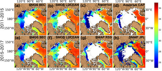
Figure 2 shows the spatial distribution of the time mean SSS during these two periods for the six satellite SSS products: SMOS BEC, SMOS LOCEAN, Aquarius, and Aquarius CAP for 2011–2015 and SMOS BEC, SMOS LOCEAN, SMAP RSS, and SMAP JPL for 2015–2017. This time mean is calculated with all the data available, whether there is one or several data available in a pixel through the whole period due to the presence of sea-ice for part of the year.
These maps show that the ice masks can be quite different among the products. In particular, the mask used in SMAP JPL data is more permissive than the other products (i.e., allowing SSS retrievals closer to ice edges). In contrast, the mask used in SMAP RSS is the most conservative among all products (i.e., excluding more SSS retrievals near ice edges). These maps also show the qualitative, large-scale consistency of the time-mean SSS fields among different SSS products and with the climatology salinity based on in-situ data from WOA13, as shown in Figure 1a. For example, the inflow of saltier Pacific waters through the Bering Strait separates the freshwater waters in the Beaufort Sea to the east and in the East Siberian Sea to the west. Both of these seas are significantly affected by river discharges. All products (except for Aquarius CAP) show a relatively sharp transition of higher salinity from the Barents Sea to lower salinity in the Kara and Laptev Seas. This reflects the influence of river discharge on the Kara and Laptev Seas and the intrusion of saltier subpolar North Atlantic waters through the Barents Sea (Aquarius CAP excluded the retrievals in the Kara Sea and Laptev Sea, so it does not show such a transition). In Baffin Bay, most products show lower SSS on western and northern parts because of Arctic Ocean outflow and river discharge, and higher salinity on the eastern and southern sides because of the intrusion of the saltier subpolar North Atlantic waters through the West Greenland Current. Despite the similarity in large-scale patterns discussed above, there are regional differences among the products. For example, SMOS LOCEAN retrievals are saltier in fresh regions, such as the Beaufort gyre, the Siberian shelf, and the Baffin Bay. The salty bias (higher than 36) observed along the east coast of Greenland is due to sea-ice contamination (personal communication from J. Boutin). Salty bias observed in SMOS LOCEAN could also be due to the use of a different dielectric constant model [39]. These differences will inform the retrieval teams to identify the underlying causes so as to improve the SSS retrievals at high latitudes.
The maps of temporal standard deviation (STD) of SSS for each of the two periods for the different products are presented in Figure 3. The standard deviation is calculated when at least 10 data values are available in a pixel through the whole period. In this figure, we chose different color scales for various products in order to visualize the spatial patterns. The temporal variability of SMOS BEC SSS is much smaller than those of other products. This is probably because in the SMOS BEC product, an objective analysis scheme with radii of 321 km, 267 km, and 175 km are applied [22]. This produces a smoothing which does not allow for capturing the small-scale variability. A new binned product is being developed at BEC under the ESA contract Arctic+, which aims at better capturing the SSS small-scale features. In contrast, the temporal variability of SMAP JPL SSS is much larger than those of other products, most likely due to the more permissive algorithm allowing retrievals near ice edges and land that are more subject to variability (e.g., runoff, sea-ice melt, and formation). However, most products, as well as the WOA13 product (Figure 1b), exhibit similar regions of high variability such as the Kara Sea, the Siberian shelf, near the mouth of the Mackenzie River, Baffin Bay, and Eastern Greenland, and the magnitudes of the STDs in these regions vary significantly among the products.
To examine consistency among different SSS products for the Arctic Ocean as a whole, we computed the monthly time series of average SSS within the Arctic Ocean (Figure 4a,b). The average was calculated for latitudes above 65°N over the ice-free ocean grid points that are common to all products for 2011–2015 (Figure 4a) and 2015–2017 (Figure 4b). These time series exhibit a seasonal cycle with minimum SSS during August–September every year (corresponding to the ice melt season) and maximum SSS during approximately December–June (corresponding to the ice freezing period). The time series also show the excellent consistency among different products at monthly time scales with regard to the interannual variation of minimum SSS: for example, the minimum SSS values during the falls of 2011 and 2012 are lower than those in 2013 and 2014. The minimum SSS values in 2017 are lower than those in 2015 and 2016. These differences do not particularly correlate with the Arctic-wide time series of September mean sea-ice extent (e.g., https://nsidc.org/arcticseaicenews/2019/09/arctic-sea-ice-reaches-second-lowest-minimum-in-satellite-record/), indicating that SSS responds to a variety of forcings from river discharge, sea-ice growth and melt, net precipitation, and ocean circulation, however this is beyond the scope of this study. The monthly spread among products (grey shadings) is about 0.43 to 0.5, which is 4 to 8 times smaller than the magnitude of the average seasonal cycle (2–4). Aquarius CAP is excluded from this figure as there is no retrieval in the Kara and Laptev Seas, affecting the seasonal and interannual variability. Therefore, the different SSS products have relatively good “signal-to-noise” ratio in representing the seasonal cycle and interannual variability of SSS averaged over the Arctic ice-free oceans.
We next compare each satellite SSS product with available in-situ data in the Arctic Ocean (Figure 5). Only observations that can be collocated with SSS satellite data (see Section 2.2 for the collocation method) are represented, i.e., there are no satellite SSS measurements retrieved under the ice, within 40 to 150 km from land (depending on the satellite product) or when sea-ice concentration or sea-ice fraction within a satellite footprint exceeds the threshold considered for each SSS product (see Data section). This map shows the striking sparseness of in-situ data in the Arctic Ocean. Over the 2011–2017 period, most of the Arctic Ocean was not sampled by in-situ instruments, only 40% of the Arctic Ocean sampled by SMAP JPL (above 65°N and considering SMAP JPL ice and land mask) has also been sampled by at least one in-situ instrument over 2011–2017. In most places sampled, the numbers of measurements are single digit, within these 40% of the area sampled, about 46% contain less than 10 in-situ observations. Some places in the Bering Strait, the Beaufort gyre, and the Barents Sea have about 50–100 measurements over the seven years. Baffin Bay and the northern Atlantic Ocean are regions that are routinely sampled with more than 500 measurements per 36 km grid cell over these seven years. The paucity of in-situ measurements poses a significant challenge to the evaluation of satellite SSS.
We first investigated the capability of satellite SSS to depict salinity gradients along TSG transects (Figure 6). We considered three different transects among the 98 transects collected. These three transects were the longest and the ones crossing the largest gradients within the two periods 2011–2015 and 2015–2017. The first transect corresponds to salinity measured all along the Arctic basin from the 19 May 2013, the second one from Denmark to northern Baffin Bay and back starting on the 31 July 2013 and the third one, also from Denmark to Baffin Bay and back, stating on the 1 June 2016. The sea-ice fraction or sea-ice concentration provided by the satellite SSS products along the transects are shown under each plot. In the three cases presented here, large gradients along the transects were well retrieved by the satellites when not contaminated by ice. Table 1 gathers all the statistics from each of the three transects. We computed in particular the correlations and the root mean square difference (RMSD) between each satellite product (when available) and in-situ measurement. Correlation coefficients are larger than 0.9 and RMSD values range from 0.2 to 2.7 for the first transect (Figure 6b, Table 1). Correlations are between 0.6 and 0.97 for the second transect and RMSD range from 0.4 to 1.4 (Figure 6d, Table 1). For the third and last transect, correlations are about 0.5 to 0.9 and RMSD range from 0.5 to 1.1 (Figure 6f, Table 1). RMSD values significantly drop for SMOS LOCEAN, SMOS BEC, and Aquarius when only considering ice fraction or sea-ice concentration values lower than 0.5% for the first transect, as well as for SMOS LOCEAN for the second and third transect (Table 1). The correlations are all significant with p-values lower than 0.05.
In the following, we compare each satellite SSS product with all the available in-situ data to examine their respective consistency with the in-situ data. Figure 7 shows the maps of RMSD between each satellite product and in-situ data per 1° bin as well as the scatter plot between each satellite SSS product and in-situ SSS. Because SMOS retrieved data from the whole study period 2011 to 2017, and because SMOS BEC provides daily data (with a 9-day running mean window), more colocations between in-situ and satellite are available for SMOS BEC (Figure 7a). SMOS LOCEAN on the other hand, only retrieves data every 4 days, so fewer colocations are available for SMOS LOCEAN than for SMOS BEC (Figure 7b). SMAP JPL is only available from 2015 to 2017 but has a relatively permissive ice mask, so more colocations are also available (Figure 7f). The RMSD between satellite and in-situ is generally larger in the Arctic Ocean than in the subpolar North Atlantic Ocean and Barents Sea, likely due to the larger gradients caused by runoff, sea-ice melting and formation, and sampling differences between in-situ and satellite observations, especially large in highly variability regions (Figure 7a–f; [36]). Also, the larger uncertainty of satellite SSS in the colder Arctic Ocean is a factor for larger differences between satellite and in-situ in the Arctic Ocean compared to the subpolar region.
The scatter plots between satellite and in-situ show that at salinities lower than 25, SMOS BEC and LOCEAN tend to overestimate SSS (Figure 2a,b,e,f; Figure 7g,h). Because of their less permissive ice masks, both Aquarius CAP and SMAP RSS do not retrieve as fresh SSS as other products (lower than 25) (Figure 7k). SMAP JPL tends to underestimate lower SSS significantly (lower than 25), this might be due to the contaminations by land and sea-ice signals (Figure 7l). From the scatter plots between each satellite SSS product and in-situ salinity, we compute the bias, RMSD, and correlations between satellite and in-situ SSS. We also compute the standard error by normalizing the standard deviation of each satellite product compared with in-situ observations by the square root of the number of samples. All the statistics are shown in Table 2. The bias between SMOS BEC and in-situ observations are relatively small compared to other products (0.08 against –0.1 to –0.6). RMSD is smaller for Aquarius CAP compared to other products, about 0.8 against 1.2 to 3.4 (Table 2). Correlation coefficients are large for all products, from 0.7 to 0.9, and are significant with p-values lower than 0.05. The standard error between satellite and in-situ is between 0.5 and 2.4. These statistics include both the uncertainties of satellite SSS and the effect of sampling differences between satellite SSS and in-situ measurements.
In order to better understand the impact of temperature and sea-ice on satellite SSS validation, in Figure 8a–f we show the average temperature (in color) per 1 × 1 bin of satellite against in-situ salinity. The largest observed differences between satellite and in-situ SSS are often associated with temperatures lower than 5 °C, especially for SMAP JPL, SMOS BEC, and SMOS LOCEAN. This shows (1) the retrieval errors in cold waters, but also (2) the impact of natural variability of SSS that is not well represented by the lack of ground truth measurements. Indeed, the SSS variability in the North Atlantic Ocean and Barents Sea where waters are warm and salty is lower compared to the higher variability in the Arctic basin, in fresh and cold waters, due to influences of runoff, ice melt, and formation. A similar analysis is done for sea-ice fraction (for Aquarius CAP and SMAP RSS) or sea-ice concentration (for SMAP JPL). In Figure 9a–c, we show the average sea-ice fraction or sea-ice concentration in percentage (color) per 1 × 1 bin of satellite against in-situ SSS. However, sea-ice fraction or concentration data are only available in Aquarius CAP, SMAP RSS, and SMAP JPL products. Because it allows more retrievals near ice edges and land, SMAP JPL exhibits the largest differences with in-situ, especially at fresher salinities. In Figure 9, we can see that the largest differences between satellite and in-situ SSS occur for larger sea-ice fraction or concentration (on average, for about 0.3% sea-ice fraction or concentration). In summary, the largest differences between in-situ and satellite are associated with lower temperature and larger sea-ice fraction or concentration.
To provide further quantitative information on the impacts of temperature and sea-ice fraction or concentration on the in-situ-satellite salinity comparisons, we analyzed the bias and RMSD between satellite and in-situ SSS as a function of the minimum temperature considered (Figure 10). There is no consistent decrease of bias as temperature increases, although two of the six products (Aquarius and SMOS LOCEAN) do have systematically lower biases as temperature increases (Figure 10a). However, there is a consistent reduction of RMSD across all products as temperature increases (Figure 10b). In other words, the STD decreases consistently as temperature increases. The implication is that biases in the satellite SSS are not necessarily related to the temperature dependence of L-band radiometric sensitivity to SSS. These results are informative to retrieval teams to investigate the factors influencing the biases. Also, increasing efforts should be dedicated to improve the dielectric constant models for cold waters.
We next investigated the relationships of biases and RMSD of the satellite SSS with maximum sea-ice fraction or concentration within the satellite footprint considered (Figure 11). As sea-ice fraction or concentration values are only available for SMAP JPL and Aquarius, we only considered these products. Note that sea-ice fraction values are also available for SMAP RSS; however, because SMAP RSS SSS are only retrieved when the sea-ice fraction within the satellite footprint is below 0.1%, we were not able to analyze the impact of the sea-ice contamination threshold on the comparison between SMAP RSS and in-situ SSS, the threshold being too low. For Aquarius CAP, RMSD between satellite and in-situ slightly increase from 0.5 to 1 with the sea-ice fraction threshold (Figure 11b), while the bias is constant (Figure 11a). For SMAP JPL, RMSD increase significantly above 0.5% of sea-ice concentration from 1.5 to 2.8 (Figure 11b), showing that considering SSS in pixels where there is more than 0.5% of sea-ice might not be reasonable. The bias however decreases from –0.7 to –0.4 (Figure 11a).

4. Discussion

Compared to previous studies, our in-situ database is much more extensive within the Arctic Ocean. In-situ data in other studies were generally biased more toward subpolar seas and the North Atlantic Ocean. One result of this new focus is that discrepancies between in-situ and satellite SSS are expected to be relatively large, owing to cold temperatures and ice contamination. In fact, we found satellite versus in-situ RMSD of 0.7–1.7 for SMOS and Aquarius, while References [19] and [20] found values generally lower than 1. Similarly, we found RMSD values of 1.5 and 3.3 for SMAP JPL and SMOS BEC matchups, while References [21] and [22] found values of 1.2 and 0.35. However, biases found in this study are between −0.6 and 0.5, which is comparable to 0.6 for SMOS in the Beaufort Sea found in Reference [23] and lower than 1, found in Reference [20] in subpolar seas.
Our study also underlines the challenges of evaluating satellite SSS, given the paucity of in-situ measurements. Enhancement of the in-situ observing system in the Arctic Ocean (e.g., Reference [40]) is important for improving satellite SSS for the Arctic Ocean. Improved satellite SSS in turn increases the sampling and coverage of the Arctic Ocean SSS field significantly, paving the way for an effective in-situ-satellite observing system for the Arctic Ocean. It is important to note that the statistics reported here for the comparison of the satellite SSS and in-situ measurements should not be interpreted as the uncertainties of the satellite SSS alone. This is because the statistics also include the effects of sampling differences between satellite SSS and in-situ measurements. Satellite SSS represent the averages within satellite footprints (ranging from about 40 km for SMOS and SMAP to 150 km for Aquarius), whereas in-situ measurements are point-wise. In regions with strong small-scale gradients (e.g., near river plumes and sea-ice edges), this difference in spatial sampling can cause significant apparent discrepancies between satellite SSS and in-situ measurements (e.g., Reference [36]). In the Arctic Ocean, where the dynamic scales are small compared with lower latitude oceans, the effect of spatial sampling differences could be further enhanced. Near-surface salinity stratification, that we have not explored in this study, can also cause differences between satellite SSS (representing the average over the top 1 cm of the ocean) and in-situ measurements (typically at the depths of meters) [36]. Unfortunately, there are insufficient in-situ salinity measurements in the upper few meters in the Arctic Ocean to examine the possible effect of the near-surface stratification. The sub-footprint horizontal SSS gradient and the vertical stratification of salinity in the Arctic Ocean are not well understood. Also, colocations between weekly satellite observations and instantaneous in-situ measurements are affected by temporal mismatch. A process experiment in the future may shed light on these processes, using, for example, a high-resolution model in which colocations with in-situ data are free from sampling differences.
Some consistent features observed by the satellite SSS products can be used to evaluate ocean and climate models, for instance, the seasonal and interannual variability of the SSS averaged over the ice-free Arctic Ocean. On the other hand, the discrepancies among different satellite SSS products provide guidance to users of the current generation of satellite SSS to evaluate the suitability of specific applications and the robustness of the results from such applications. Finally, our results provide important feedback to the satellite SSS retrieval teams to work collaboratively to improve the products (e.g., investigating the cause for and reducing the biases, sea-ice corrections). Indeed, more in-situ data are needed in order to better evaluate SSS products near sea-ice edges (1%–3% ice fraction up to 15%) during different seasons based on level 2 SSS data. A strategy within the different retrieval teams is needed to develop in-situ campaign in the Arctic to allow a more robust validation of satellite SSS products in the Arctic.

5. Conclusions

This study presented a systematic analysis of six commonly used satellite SSS products from three different satellite missions (SMOS, Aquarius, and SMAP), including two products from each of these missions. Overall, the satellite SSS products provide a similar characterization of the large-scale patterns of the time mean SSS (Figure 2). They are also relatively consistent in depicting the regions with strong temporal variability of SSS (Figure 3). When averaged over the Arctic Ocean, the satellite SSS show an excellent consistency in describing the seasonal and interannual variation of the SSS (Figure 4). In particular, the average spread among products for the Arctic-Ocean averages (0.4–0.5) were much lower than the magnitudes of the seasonal cycle (2–4). Comparison of satellite SSS with in-situ salinity measurements along TSG transects suggested that satellite SSS are able to capture the salinity gradient away from regions with significant sea-ice concentration (i.e., ice fraction or sea-ice concentration larger than 0.5%) (Figure 6, Table 1). Overall, the RMSD of satellite SSS with respect to available in-situ measurements in the Arctic Ocean improves with increasing temperature, which reflects the low sensitivity of L-band radiometry to SSS in cold waters (Figure 10). However, the lack of in-situ data to represent the higher natural variability of SSS in fresh and cold regions in the Arctic Ocean compared to the warm and salty regions of the Barents Sea has to be taken into consideration to interpret these results. On the other hand, the bias of satellite SSS with respect to in-situ measurements does not show a consistent dependence on temperature, suggesting that further investigation is needed to understand the causes of satellite SSS bias. More in-situ salinity measurements in the ice-free Arctic Ocean are clearly important to improve the assessment and retrievals of satellite SSS in the Arctic Ocean, especially in the upper meter. Moreover, an intercomparison of satellite SSS retrievals from different satellites using consistent ancillary data, such as sea ice mask, SST, and wind, as well as a dielectric model, would be very helpful in identifying the causes for the discrepancies of satellite SSS reported in this study.

Author Contributions

Conceptualization, S.F.; methodology, S.F., M.S. and W.T.; validation, S.F.; formal analysis, S.F.; investigation, S.F.; data curation, S.F. and M.S.; writing—original draft preparation, S.F.; writing—review and editing, T.L., M.S., W.T., E.O.; funding acquisition, T.L.

Funding

The research described in this paper was carried out at the Jet Propulsion Laboratory, California Institute of Technology, under a contract with NASA. This research was supported by a NASA grant. M. Steele was also supported by NASA grant 80NSSC18K0837, ONR grant N00014-17-1-2545, and NSF grant OPP-1751363.

Acknowledgments

We thank the following for in-situ observations: Andrey Proshutinksy and Richard Krishfield (Woods Hole Oceanographic Institute; WHOI) in collaboration with Fisheries and Oceans Canada at the Institute of Ocean Sciences for Beaufort Gyre Exploration Project ship CTD data (https://www.whoi.edu/beaufortgyre); Igor Polyakov (University of Alaska, Fairbanks) for ship CTD data (https://uaf-iarc.org/nabos/); Craig Lee and Luc Rainville (Applied Physics Laboratory; APL, University of Washington; UW) for glider CTD data from the ONR MIZ DRI project (http://www.apl.washington.edu/project/project.php?id=miz); Luc Rainville and Jim Thomson (APL/UW) for underway CTD data from the ONR Seastate DRI project (http://www.apl.washington.edu/arcticseastate); Craig Lee and Jason Gobat (APL/UW) for ship CTD data from the NSF Davis Strait project (http://iop.apl.washington.edu/projects/ds/html/program.html; NSF grant ARC1022472); Sarah Dewey and James Morison (Polar Science Center; PSC, APL/UW) for Air-expendable CTD data from the ONR SIZRS project http://psc.apl.uw.edu/research/projects/sizrs; Ignatius Rigor and Bonnie Light (PSC/APL/UW) and Victoria Hill (Old Dominion University) for temperature and salinity data from surface drifting buoys (http://iabp.apl.washington.edu; http://psc.apl.washington.edu/UpTempO/); Sarah Webster (APL/UW) and Lora Van Uffelen (University of Rhode Island) for glider CTD data from the ONR CANAPE/CABAGE DRI project (https://scripps.ucsd.edu/research/proposals/canada-basin-acoustic-propagation-experiment-canape); Kevin Wood (UW and NOAA/PMEL) and Steve Jayne (WHOI) for Alamo float CTD data from the NOAA Arctic Heat and ONR SODA DRI projects (https://www.pmel.noaa.gov/arctic-heat/data); Humfrey Melling (Institute for Ocean Sciences) for TSG data from the Canadian Program on Energy Research and Development’s Beaufort Marine Hazards project (http://science.gc.ca/eic/site/063.nsf/eng/h_935CCA80.html); Marion Alberty, Jennifer MacKinnon, and Matthew Alford (Scripps Institute of Oceanography), and John Mickett (APL/UW) for TSG data from the NSF Arctic Mix project (http://icefloe.net/files/Sikuliaq%202015%20MacKinnon%20arcticmix_cruise_report_reduced.pdf); Paul Dodd (Norwegian Polar Institute) for ship CTD data from the Fram Strait Arctic Ocean Outflow Observatory project (http://www.npolar.no/en/projects/fram-strait-arctic-outflow-observatory.html); and Sigrid Lind (Institute of Marine Research) for ship CTD data (https://www.imr.no/en). We also acknowledge the CLIVAR and Carbon Hydrographic Data Office for TSG data (https://cchdo.ucsd.edu/search?bbox=-180,65,180,90); the Global Ocean Surface Underway Data (GOSUD) hosted by Coriolis for TSG data (http://www.coriolis.eu.org/Data-Products/Catalogue#/metadata/81117be9-7b90-4bab-9082-702301323028); PANGAEA for the diverse data collected (https://doi.pangaea.de/10.1594/PANGAEA.872931); LEGOS for TSG data (http://sss.sedoo.fr/#); Coriolis center for diverse salinity in-situ data (http://www.coriolis.eu.org/Data-Products/Data-Delivery/Data-selection); the World Ocean Atlas 13 salinity data; CNES-IFREMER Centre Aval de Traitement des Données SMOS (CATDS) for the SMOS LOCEAN SSS data; the Barcelona Expert Center (BEC) for the SMOS BEC SSS dedicated to the high latitudes; the NASA Physical Oceanography Distributed Active Archive Center (PO.DAAC) for the Aquarius and SMAP SSS data.

Conflicts of Interest

The authors declare no conflict of interest. The funders had no role in the design of the study; in the collection, analyses, or interpretation of data; in the writing of the manuscript, or in the decision to publish the results.

References

  1. Aagaard, K.; Coachman, L.K.; Carmack, E. On the halocline of the Arctic Ocean. Deep Sea Res. Part A Oceanogr. Res. Pap. 1981, 28, 529–545. [Google Scholar] [CrossRef]
  2. Carmack, E.C. The alpha/beta ocean distinction: A perspective on freshwater fluxes, convection, nutrients and productivity in high-latitude seas. Deep Sea Res. Part II Top. Stud. Oceanogr. 2007, 54, 2578–2598. [Google Scholar] [CrossRef]
  3. Talley, L.D. Salinity patterns in the ocean. In Encyclopedia of Global Change. Volume: The Earth System: Physical and Chemical Dimensions of Global Environmental Change; MacCracken, M.C., Perry, J.S., Eds.; John Wiley & Sons, Ltd.: Chichester, UK, 2002; pp. 629–640. [Google Scholar]
  4. Solomon, S.; Qin, D.; Manning, M.; Marquis, L.; Averyt, K.; Tignor, M.M.B.; LeRoy Miller, H.; Chen, Z. IPCC Climate Change 2013: The Physical Science Basis. In Working Group 1 Contribution to the Fourth Assessment Report of the Intergovernmental Panel on Climate Change; Cambridge University Press: Cambridge, UK, 2013; p. 1535. [Google Scholar]
  5. Chen, X.Y.; Tung, K.-K. Varying planetary heat sink led to global-warming slowdown and acceleration. Science 2014, 345, 897–903. [Google Scholar] [CrossRef] [PubMed]
  6. Pivovarov, S.; Schlitzer, R.; Novikhin, A. River runoff influence on the water mass formation in the Kara Sea. In Siberian River Run-Off in the Kara Sea: Characterization, Quantification, Variability, and Environmental Significance; Elsevier: Amsterdam, The Netherlands, 2003; Volume 6, pp. 9–26. [Google Scholar]
  7. Li, W.K.; McLaughlin, F.A.; Lovejoy, C.; Carmack, E.C. Smallest algae thrive as the Arctic Ocean freshens. Science 2009, 326, 539. [Google Scholar] [CrossRef] [PubMed] [Green Version]
  8. Carmack, E.; Polyakov, I.; Padman, L.; Fer, I.; Hunke, E.; Hutchings, J.; Jackson, J.; Kelley, D.; Kwok, R.; Layton, C.; et al. Toward quantifying the increasing role of oceanic heat in sea-ice loss in the New Arctic. Bull. Am. Meteorol. Soc. 2015, 96, 2079–2105. [Google Scholar] [CrossRef]
  9. Polyakov, I.V.; Beszczynska, A.; Carmack, E.C.; Dmitrenko, I.A.; Fahrbach, E.; Frolov, I.E.; Gerdes, R.; Hansen, E.; Holfort, J.; Ivanov, V.V.; et al. One more step toward a warmer Arctic. Geophys. Res. Lett. 2005, 32, L17605. [Google Scholar] [CrossRef] [Green Version]
  10. Kwok, R.; Rothrock, D.A. Decline in Arctic sea-ice thickness from submarine and ICES at records: 1958–2008. Geophys. Res. Lett. 2009, 36, L15501. [Google Scholar] [CrossRef] [Green Version]
  11. McPhee, M.G.; Proshutinsky, A.; Morison, J.H.; Steele, M.; Alkire, M.B. Rapid change in freshwater content of the Arctic Ocean. Geophys. Res. Lett. 2009, 36, L10602. [Google Scholar] [CrossRef] [Green Version]
  12. Kerr, Y.H.; Waldteufel, P.; Wigneron, J.P.; Delwart, S.; Cabot, F.; Boutin, J.; Escorihuela, M.J.; Font, J.; Reul, N.; Gruhier, C.; et al. The SMOS mission: New tool for monitoring key elements of the global water cycle. Proc. IEEE 2010, 98, 666–687. [Google Scholar] [CrossRef] [Green Version]
  13. Mecklenburg, S.; Drusch, M.; Kerr, Y.; Font, J.; Martin-Neira, M.; Delwart, S.; Buenadicha, G.; Reul, N.; Daganzo-Eusebio, E.; Oliva, R.; et al. ESA’s Soil Moisture and Ocean Salinity Mission: Mission Performance and Operations. IEEE Trans. Geosci. Remote Sens. 2012, 50, 1354–1366. [Google Scholar] [CrossRef] [Green Version]
  14. Lagerloef, G.; Colomb, F.R.; Le Vine, D.; Wentz, F.; Yueh, S.; Ruf, C.; Lilly, J.; Gunn, J.; Chao, Y.; deCharon, A.; et al. The Aquarius/SAC-D mission—Designed to Meet the Salinity Remote Sensing Challenge. Oceanogr. Mag. 2008, 21, 68–81. [Google Scholar] [CrossRef] [Green Version]
  15. Entekhabi, D.; Das, N.; Yueh, S.; De Lannoy, G.; O’Neill, P.E.; Dunbar, R.S.; Kellogg, K.H.; Edelstein, W.N.; Allen, A.; Entin, J.K.; et al. SMAP Handbook. Jet Propulsion Laboratory Publ. 400-1567; p. 182. 2014. Available online: https://smap.jpl.nasa.gov/system/internal_resources/details/original/178_SMAP_Handbook_FINAL_1_JULY_2014_Web.pdf (accessed on 12 November 2019).
  16. Swift, C.; McIntosh, R. Considerations for microwave remote sensing of ocean-surface salinity. IEEE Trans. Geosci. Electron. 1983, 21, 480–491. [Google Scholar] [CrossRef]
  17. Yueh, S.; West, R.; Wilson, W.; Li, F.; Nghiem, S.; Rahmat-Samii, Y. Error sources and feasibility for microwave remote sensing of ocean surface salinity. IEEE Trans. Geosci. Remote Sens. 2001, 39, 1049–1059. [Google Scholar] [CrossRef] [Green Version]
  18. Carmack, E.; Winsor, P.; Williams, W. The contiguous panarctic riverine coastal domain: A unifying concept. Prog. Oceanogr. 2015, 139, 13–23. [Google Scholar] [CrossRef]
  19. Köhler, J.; Martins, M.S.; Serra, N.; Stammer, D. Quality assessment of spaceborne sea surface salinity observations over the northern North Atlantic. J. Geophys. Res. Oceans 2015, 120, 94–112. [Google Scholar] [CrossRef] [Green Version]
  20. Garcia-Eidell, C.; Comiso, J.C.; Dinnat, E.; Brucker, L. Satellite observed salinity distributions at high latitudes in the Northern Hemisphere: A comparison of four products. J. Geophys. Res. Ocean. 2017, 122, 7717–7736. [Google Scholar] [CrossRef] [Green Version]
  21. Tang, W.; Yueh, S.; Yang, D.; Fore, A.; Hayashi, A.; Lee, T.; Fournier, S.; Holt, B. The potential and challenges of using Soil Moisture Active Passive (SMAP) sea surface salinity to monitor Arctic Ocean freshwater changes. Remote Sens. 2018, 10, 869. [Google Scholar] [CrossRef] [Green Version]
  22. Olmedo, E.; Gabarró, C.; González-Gambau, V.; Martínez, J.; Ballabrera-Poy, J.; Turiel, A.; Portabella, M.; Fournier, S.; Lee, T. Seven years of SMOS sea surface salinity at high latitudes: Variability in Arctic and Sub-Arctic regions. Remote Sens. 2018, 10, 1772. [Google Scholar] [CrossRef] [Green Version]
  23. Xie, J.; Raj, R.P.; Bertino, L.; Samuelsen, A.; Wakamatsu, T. Evaluation of Arctic Ocean surface salinities from the Soil Moisture and Ocean Salinity (SMOS) mission against a regional reanalysis and in situ data. Ocean Sci. 2019, 15, 1191–1206. [Google Scholar] [CrossRef] [Green Version]
  24. Kubryakov, A.; Stanichny, S.; Zatsepin, A. River plume dynamics in the Kara Sea from altimetry-based lagrangian model, satellite salinity and chlorophyll data. Remote Sens. Environ. 2016, 176, 177–187. [Google Scholar] [CrossRef]
  25. Matsuoka, A.; Babin, M.; Devred, E.C. A new algorithm for discriminating water sources from space: A case study for the southern Beaufort Sea using MODIS ocean color and SMOS salinity data. Remote Sens. Environ. 2016, 184, 124–138. [Google Scholar] [CrossRef]
  26. Boutin, J.; Jean-Luc, V.; Dmitry, K. SMOS SSS L3 maps generated by CATDS CEC LOCEAN, debias V3.0. SEANOE. 2018. Available online: https://www.seanoe.org/data/00417/52804/ (accessed on 12 November 2019). [CrossRef]
  27. Yueh, S.H.; Tang, W.; Hayashi, A.K.; Lagerloef, G.S.E. L-band passive and active microwave geophysical model functions of ocean surface winds and applications to aquarius retrieval. IEEE Trans. Geosci. Remote Sens. 2014, 51, 4619–4632. [Google Scholar] [CrossRef]
  28. Lee, T.; Lagerloef, G.; Gierach, M.M.; Kao, H.Y.; Yueh, S.; Dohan, K. Aquarius reveals salinity structure of tropical instability waves. Geophys. Res. Lett. 2012, 39, 12610. [Google Scholar] [CrossRef]
  29. Fore, A.G.; Yueh, S.H.; Tang, W.; Stiles, B.W.; Hayashi, A.K. Combined active/passive retrievals of ocean vector wind and sea surface salinity with SMAP. IEEE Trans. Geosci. Remote Sens. 2016, 54, 7396–7404. [Google Scholar] [CrossRef]
  30. Meissner, T.; Wentz, F.; Le Vine, D. The salinity retrieval algorithms for the NASA Aquarius version 5 and SMAP version 3 releases. Remote Sens. 2018, 10, 1121. [Google Scholar] [CrossRef] [Green Version]
  31. Meissner, T.; Wentz, F. The complex dielectric constant of pure and sea water from microwave satellite observations. IEEE Trans. Geosci. Remote Sens. 2004, 42, 1836–1849. [Google Scholar] [CrossRef] [Green Version]
  32. Klein, L.; Swift, C. An improved model for the dielectric constant of sea water at microwave frequencies. IEEE Trans. Antennas Propag. 1977, AP-25, 104–111. [Google Scholar] [CrossRef]
  33. Dinnat, E.P.; Brucker, L. Improved sea-ice fraction characterization for L-band observations by the aquarius radiometers. IEEE Trans. Geosci. Remote Sens. 2016, 55, 1285–1304. [Google Scholar] [CrossRef]
  34. Behrendt, A.; Sumata, H.; Rabe, B.; Schauer, U. A Comprehensive, Quality-Controlled and Up-to-Date Data Set of Temperature and Salinity Data for the Arctic Mediterranean Sea (Version 1.0). PANGAEA. 2017. Available online: https://doi.pangaea.de/10.1594/PANGAEA.872931 (accessed on 12 November 2019). [CrossRef]
  35. Cabanes, C.; Grouazel, A.; von Schuckmann, K.; Hamon, M.; Turpin, V.; Coatanoan, C.; Paris, F.; Guinehut, C.; Boone, C.; Ferry, N.; et al. The CORA dataset: Validation and diagnostics of in-situ ocean temperature and salinity measurements. Ocean Sci. 2013, 9, 1–18. [Google Scholar] [CrossRef] [Green Version]
  36. Boutin, J.; Chao, Y.; Asher, W.E.; Delcroix, T.; Drucker, R.; Drushka, K.; Kolodziejczyk, N.; Lee, T.; Reul, N.; Reverdin, G.; et al. Satellite and in-situ salinity: Understanding near-surface stratification and subfootprint variability. Bull. Am. Meteorol. Soc. 2016, 97, 1391–1407. [Google Scholar] [CrossRef] [Green Version]
  37. Vinogradova, N.T.; Ponte, R.M. Assessing temporal aliasing in satellite-based salinity measurements. J. Atmos. Ocean. Technol. 2012, 29, 1391–1400. [Google Scholar] [CrossRef]
  38. Zweng, M.M.; Reagan, J.R.; Seidov, D.; Boyer, T.P.; Locarnini, R.A.; Garcia, H.E.; Mishonov, A.V.; Baranova, O.K.; Weathers, K.; Paver, C.R.; et al. World Ocean Atlas 2018, Volume 2: Salinity; Mishonov, A., Ed.; NOAA Atlas NESDIS: Silver Spring, MD, USA, 2018; Volume 82, p. 50.
  39. Dinnat, E.P.; Boutin, J.; Yin, X.; Le Vine, D.M. Inter-comparison of SMOS and aquarius sea surface salinity: Effects of the dielectric constant and vicarious calibration. In Proceedings of the 13th Specialist Meeting on Microwave Radiometry and Remote Sensing of the Environment (MicroRad), Pasadena, CA, USA, 24–27 March 2014; pp. 55–60. [Google Scholar]
  40. Lee, C.M.; Starkweather, S.; Eicken, H.; Timmermans, M.L.; Wilkinson, J.; Sandven, S.; Dukhovskoy, D.; Gerland, S.; Grebmeier, J.M.; Intrieri, J.; et al. A framework for the development, design and implementation of a sustained Arctic Ocean observing system. Front. Mar. Sci. 2019, 6, 451. [Google Scholar] [CrossRef] [Green Version]
Figure 1. (a) Annual mean of salinity from World Ocean Atlas 13, on top of which are represented the main areas of interest discussed in the study. (b) Standard deviation of the monthly mean of salinity from World Ocean Atlas 13, the main Arctic Rivers are shown on the map. A logarithmic scale is used for the standard deviation map (b).
Remotesensing 11 03043 g001
Figure 2. Annual mean of sea surface salinity (SSS) over (ad) 2011–2015 and (eh) 2015–2017 from (a,e) SMOS BEC, (b,f) SMOS LOCEAN, (c) Aquarius, (d) Aquarius CAP, (g) SMAP RSS, and (h) SMAP JPL.
Remotesensing 11 03043 g002
Figure 3. Annual standard deviation of SSS over (ad) 2011–2015 and (eh) 2015–2017 from (a,e) SMOS BEC, (b,f) SMOS LOCEAN, (c) Aquarius, (d) Aquarius CAP, (g) SMAP RSS, and (h) SMAP JPL. Note the different colorbar amplitudes (0–1.5 for SMOS BEC, 0–4 for SMOS LOCEAN, Aquarius, Aquarius CAP, and SMAP RSS, 0–10 for SMAP JPL).
Remotesensing 11 03043 g003
Figure 4. (a,b) Monthly time series of satellite sea surface salinity in the Arctic Basin over 65°N. The black dotted line represents the average over the SSS products available, the shading represents the spread of SSS products around the average. The spread is computed as the average of the standard deviation between two products.
Remotesensing 11 03043 g004
Figure 5. Number of in-situ observations from 2011 to 2017 available to colocate with satellite SSS observations within the upper 10 meters per 36 km grid cell (EASE36).
Remotesensing 11 03043 g005
Figure 6. (a,d,g) SMOS BEC SSS maps of 19 May 2013, 31 July 2013, and 1 June 2016 respectively, on top of which, represented as a black solid line, is the TSG transect trajectory starting on each of these days respectively. (b,e,h) SSS from in-situ (black), SMOS BEC (cyan), SMOS LOCEAN (red), Aquarius (green), Aquarius CAP (yellow), SMAP JPL (blue), and SMAP RSS (magenta) along the transect represented on the maps on the left. The ice fraction (in %) from Aquarius CAP, SMAP JPL, or SMAP RSS products along the transect are represented underneath each transect (c,f,i).
Remotesensing 11 03043 g006
Figure 7. (af) Maps of root mean square difference (RMSD) per 1° bin between in-situ observations and satellite SSS from (a) SMOS BEC, (b) SMOS LOCEAN, (c) Aquarius, (d) Aquarius CAP, (e) SMAP RSS, and (f) SMAP JPL. (gl) Scatter plots of satellite SSS ((g) SMOS BEC, (h) SMOS LOCEAN, (i) Aquarius, (j) Aquarius CAP, (k) SMAP RSS, and (l) SMAP JPL) against in-situ SSS per 1° bin factor for larger differences between satellite and in-situ in the Arctic Ocean compared to the subpolar region.
Remotesensing 11 03043 g007
Figure 8. Scatter plots of satellite SSS ((a) SMOS BEC, (b) SMOS LOCEAN, (c) Aquarius, (d) Aquarius CAP, (e) SMAP RSS, and (f) SMAP JPL) against in-situ salinity per 1° bin. The colors represent the mean temperature per 1 × 1.
Remotesensing 11 03043 g008
Figure 9. Scatter plots of satellite SSS ((a) Aquarius CAP, (b) SMAP RSS, and (c) SMAP JPL) against in-situ salinity per 1° bin. The colors represent the mean sea-ice fraction per 1 × 1. For better visualization, we used a logarithmic scale.
Remotesensing 11 03043 g009
Figure 10. (a) Bias and (b) RMSD between in-situ observations and satellite SSS of SMOS BEC (cyan), SMOS LOCEAN (red), Aquarius (green), Aquarius CAP (orange), SMAP RSS (magenta), and SMAP JPL (blue) per 1° bin as a function of the minimum temperature considered.
Remotesensing 11 03043 g010
Figure 11. (a) Bias and (b) RMSD between in-situ observations and satellite SSS of Aquarius CAP (orange) and SMAP JPL (blue) per 1° bin as a function of a maximum sea-ice concentration considered.
Remotesensing 11 03043 g011
Table 1. Root mean square difference (RMSD) and correlation coefficients between each satellite and in-situ salinity along each of the three transects represented in Figure 5. The RMSD values within parenthesis corresponds to the RMSD values when SSS values for which ice fraction is lower than 0.5% are considered. The p-value significance of the correlations is shown within parenthesis.
Transect 1Transect 2Transect 3
RMSD (Ice Fraction < 0.5%)Correlation (p-Value Significance)RMSD (Ice Fraction < 0.5%)Correlation (p-Value Significance)RMSD (Ice Fraction < 0.5%)Correlation (p-Value Significance)
SMOS LOCEAN2.06 (0.59)0.91 (<0.0001)1.47 (1.3)0.56 (<0.0001)1.13 (1.04)0.53 (<0.0001)
SMOS BEC1.63 (1.12)0.91 (<0.0001)0.78 (0.8)0.85 (<0.0001)1.02 (1.03)0.85 (<0.0001)
Aquarius2.71 (1.42)0.93 (<0.0001)0.61 (0.61)0.88 (<0.0001)N/AN/A
Aquarius CAP0.27 (0.27)0.97 (<0.0001)0.38 (0.38)0.97 (<0.0001)N/AN/A
SMAP JPLN/AN/AN/AN/A1.45 (1.43)0.80 (<0.0001)
SMAP RSSN/AN/AN/AN/A0.52 (0.52)0.88 (<0.0001)
Table 2. Bias, RMSD, correlation coefficients, and standard error between each satellite product and in situ SSS above 65°N.
BiasRMSDCorrelation (p-Value Significance)Standard Error
SMOS LOCEAN−0.611.700.88 (<0.0001)1.12
SMOS BEC0.081.510.91 (<0.0001)1.07
Aquarius0.561.630.91 (<0.0001)1.09
Aquarius CAP−0.240.770.95 (<0.0001)0.52
SMAP JPL−0.123.370.76 (<0.0001)2.38
SMAP RSS−0.161.200.93 (<0.0001)0.84

