An Object-Based Strategy for Improving the Accuracy of Spatiotemporal Satellite Imagery Fusion for Vegetation-Mapping Applications

Abstract

Spatiotemporal data fusion is a key technique for generating unified time-series images from various satellite platforms to support the mapping and monitoring of vegetation. However, the high similarity in the reflectance spectrum of different vegetation types brings an enormous challenge in the similar pixel selection procedure of spatiotemporal data fusion, which may lead to considerable uncertainties in the fusion. Here, we propose an object-based spatiotemporal data-fusion framework to replace the original similar pixel selection procedure with an object-restricted method to address this issue. The proposed framework can be applied to any spatiotemporal data-fusion algorithm based on similar pixels. In this study, we modified the spatial and temporal adaptive reflectance fusion model (STARFM), the enhanced spatial and temporal adaptive reflectance fusion model (ESTARFM) and the flexible spatiotemporal data-fusion model (FSDAF) using the proposed framework, and evaluated their performances in fusing Sentinel 2 and Landsat 8 images, Landsat 8 and Moderate-resolution Imaging Spectroradiometer (MODIS) images, and Sentinel 2 and MODIS images in a study site covered by grasslands, croplands, coniferous forests, and broadleaf forests. The results show that the proposed object-based framework can improve all three data-fusion algorithms significantly by delineating vegetation boundaries more clearly, and the improvements on FSDAF is the greatest among all three algorithms, which has an average decrease of 2.8% in relative root-mean-square error (rRMSE) in all sensor combinations. Moreover, the improvement on fusing Sentinel 2 and Landsat 8 images is more significant (an average decrease of 2.5% in rRMSE). By using the fused images generated from the proposed object-based framework, we can improve the vegetation mapping result by significantly reducing the “pepper-salt” effect. We believe that the proposed object-based framework has great potential to be used in generating time-series high-resolution remote-sensing data for vegetation mapping applications.

1. Introduction

Mapping the distribution and quantity of vegetation is critical for managing natural resources, preserving biodiversity, estimating vegetation carbon storage, and understanding the Earth’s energy balance [1]. Remote-sensing technology has been proven to be an efficient and economical tool for mapping vegetation types and cover at large spatial scales [2,3]. However, the spectral similarities among different land surface objects and different vegetation types have been a major factor influencing the accuracy of vegetation mapping [4]. Because vegetation phenology information provided by multi-temporal images with a finer spatial resolution is beneficial for improving vegetation mapping accuracy [5,6], the derivation and processing of multi-temporal remote-sensing data with a high spatial resolution have been an active research area in the field of vegetation mapping.

Given the tradeoff between spatial resolution and temporal revisiting cycles [7], current satellite images have either high spatial resolutions but low temporal resolutions (e.g., Landsat, Sentinel 2) or low spatial resolutions but high temporal resolutions (e.g., Moderate-resolution Imaging Spectroradiometer (MODIS), Sentinel-3). Moreover, cloud contaminations can further increase the fragmentation of satellite remote-sensing data [8]. Spatiotemporal data fusion, a methodology for fusing satellite images from two different sensors, has been developed to generate data with both high spatial and temporal resolutions [9]. Conventionally, in spatiotemporal data fusion, imagery with a high spatial resolution but low temporal resolution is called “fine imagery”, while imagery with a low spatial resolution but high temporal resolution is called “coarse imagery” [10], which is being followed in this study.

So far, many spatiotemporal data-fusion algorithms have been developed, and they can be generally divided into five categories (i.e., unmixed-based, weight function-based, Bayesian-based, learning-based, and hybrid methods) [11]. Nevertheless, most of these methods have a common key step, which is to find similar pixels from the fine imagery. These similar pixels from the fine imagery are used to predict the fused value and reduce the prediction uncertainty caused by noise [12]. For example, the spatial and temporal adaptive reflectance fusion model (STARFM) uses the spectral similarity and spatial distance as constrains to select similar pixels within a defined search window and predict the reflectance value of a target pixel by using the linear weighted method [13]. The enhanced spatial and temporal adaptive reflectance fusion model (ESTARFM) also uses spectral similarity to select initial similar pixels in two fine images acquired at different times, and further constrains the selection results by only using the similar pixels found in both images [12]. The flexible spatiotemporal data-fusion model (FSDAF) uses auxiliary land-cover classification information to help determine the similar pixels by ensuring they have the same land cover type as the target pixel [14]. The performance of all above-mentioned methods is highly influenced by the similar pixel selection accuracy since wrong similar pixels can lead to errors in the final spatiotemporal fusion results [15].

Currently, the similar pixel selection methods based on spectral similarity satisfy the requirements for applications such as land-cover mapping [16], since the spectral differences among different land cover types are observable. However, these methods may not perform well when they are used in vegetation-mapping applications. Differences in spectral reflectance are much smaller among vegetation types than among land cover types [2], and spectral similarity-based methods (e.g., STARFM and ESTARFM) may lead to many wrong similar pixels. These misidentified similar pixels may result in blurring effects at the boundaries among vegetation types in the fused images and, therefore, cause vegetation mapping errors. Moreover, the vegetation classification map required by the methods using auxiliary classification information (e.g., FSDAF) is not available in most applications. How to accurately identify similar pixels from fine imagery is still a challenging task for spatiotemporal fusion in vegetation mapping applications.

In addition to spectral information, image textures have been shown to be another useful type of information for vegetation mapping [17,18]. Different compositions of vegetation types may have significant differences in textures, which can help separating adjacent vegetation types [19,20]. The object-based image analysis (OBIA) method is one of the several approaches utilizing image textures [21]. OBIA incorporates texture information, spectral information and context structure to segment the image into homogeneous objects [22]. Each segmented object from OBIA can be treated as a thematic class, e.g., vegetation type, which provides a potential candidate pool for selecting similar pixels. Therefore, using the OBIA segmented objects as a constraint beyond spectral similarity might provide a more accurate set of similar pixels that have the same vegetation type as the target pixel. However, to the best of our knowledge, the effectiveness of OBIA in similar pixel selection has not yet been tested, although the consensus for advantages of OBIA has been achieved among numerous researchers.

This study describes and tests an object-based spatiotemporal data-fusion framework that uses an additional constraint for selecting similar pixels from segmented objects. To evaluate the proposed framework, we implemented the object-based improvement in the three widely used spatiotemporal data-fusion algorithms, i.e., STARFM, ESTARFM and FSDAF and tested their performance.

2. Methodology

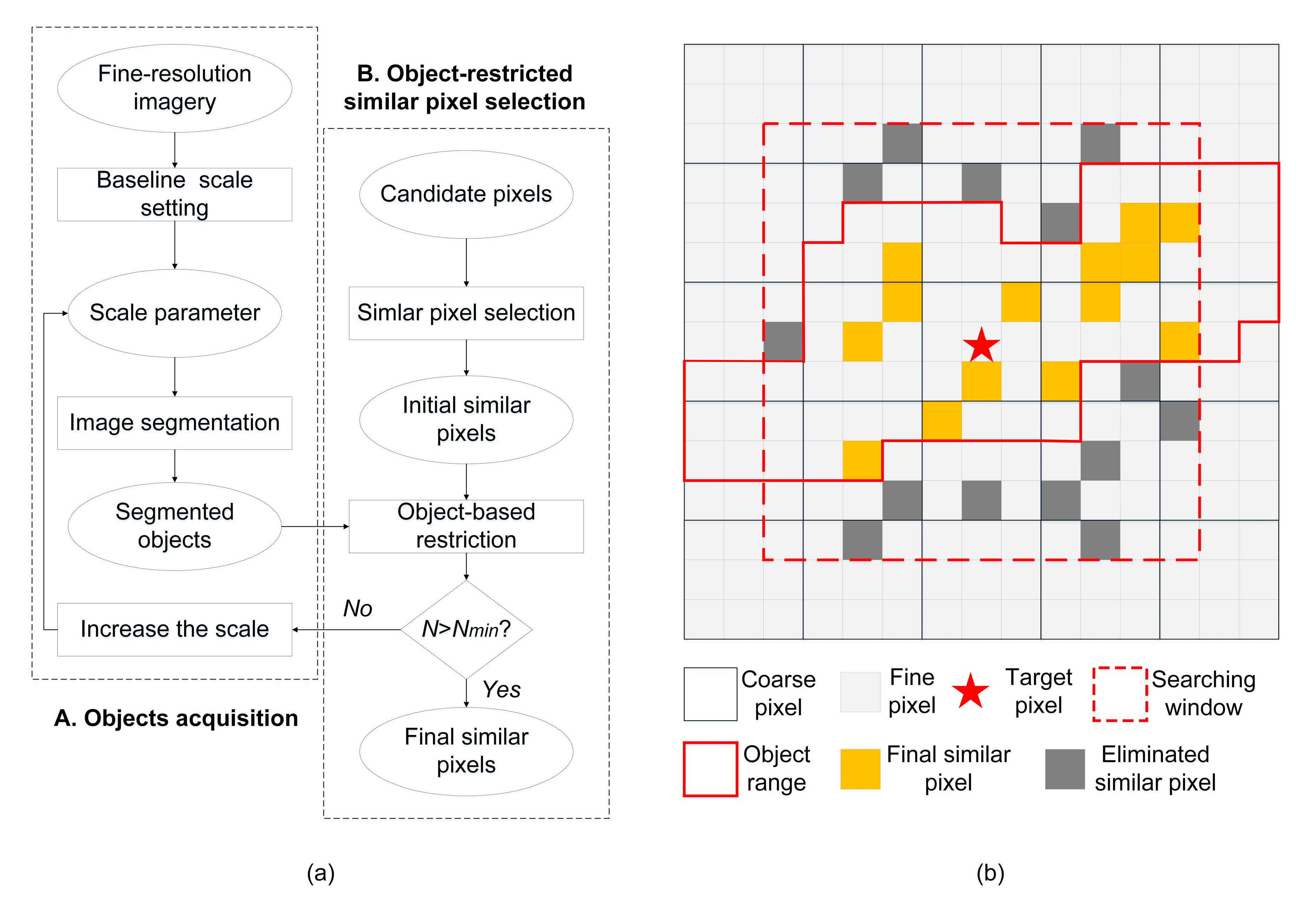
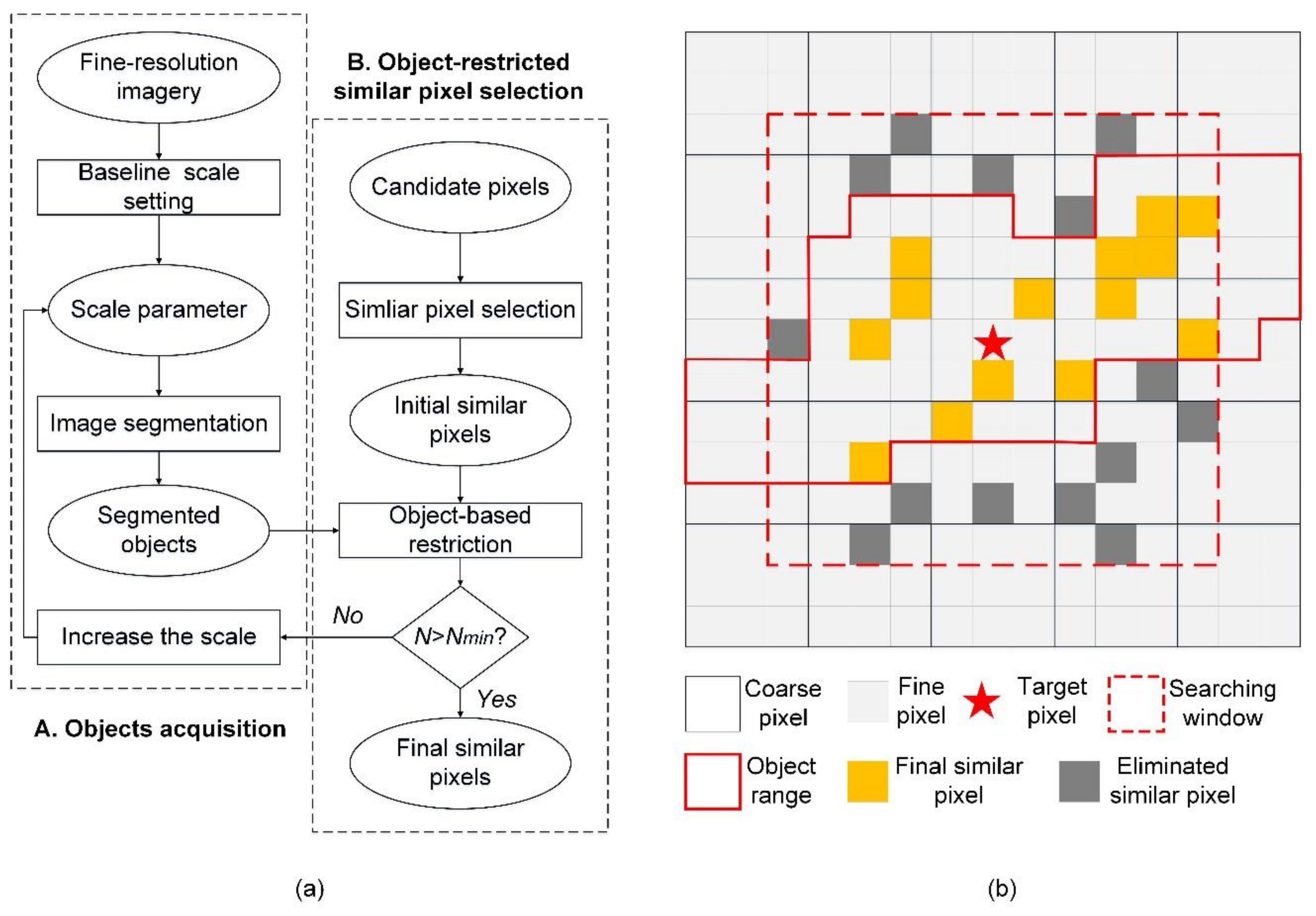
Although most current spatiotemporal fusion algorithms differ greatly in principle, they share the same four implementation steps: (i) initial prediction; (ii) selection of similar pixels; (iii) calculation of weighting coefficients of similar pixels; (iv) final prediction based on similar pixels. These steps can be described as follows: first, the value of each fine pixel is estimated at the predicted date through temporal/spatial dependence; next, pixels similar to each fine pixel are selected; then, the weight of each similar pixel is calculated based on the spectral/spatial distance; lastly, the weighted sum of similar pixels is used to predict the final value of each fine pixel. In this study, the proposed framework shares the same four steps mentioned above. To reduce the uncertainty brought by selecting the wrong similar pixels in step (ii), we integrated an object-restricted similar pixel selection method (Figure 1). Any spatiotemporal fusion algorithms sharing the same four steps described above (e.g., STARFM, ESTARFM and FSDAF) can use this framework by replacing step (ii) with the proposed method. Details of the object-restricted similar pixel selection process are introduced as follows.

Defining objects through image segmentation is the basis of the object-restricted similar pixel selection (Figure 1a). For the proposed framework, it is critical to set a suitable scale for the image segmentation process because too small a scale can lead to a small object size that might result in an insufficient number of similar pixels, and an excessively large scale might decrease the homogeneity within an object. To determine the optimal segmentation scale, this study uses the improved Estimation of Scale Parameter tool (ESP2) developed by Drăguţ et al. [23], an optimal scale selection method that can simultaneously minimize the intrasegment homogeneity and maximize the intersegment heterogeneity [24]. Three optimal segmentation scales, from small to large (i.e., Level 1, Level 2 and Level 3), are provided by the ESP2 tool, and the smallest optimal scale Level 1 is used as the baseline scale to start the similar pixel selection process.

With the determined baseline scale, the multiresolution segmentation method is used to segment the input fine image into objects. After segmentation, each pixel is exclusively assigned to an object and gets a corresponding object identification. The rule of the proposed object-restricted similar pixel selection can be described as follows:

$$\left\{\begin{array}{c}\left|F\left(x_i,y_j,b\right)-F\left(x_{w/2},y_{w/2},b\right)\right|\le T_s\\ O\left(x_i,y_j\right)-O\left(x_{w/2},y_{w/2}\right)=0\end{array}\right.$$

(1)

where F refers to the fine imagery at the input time; $b$ refers to the bth band; ($x_i,y_j$) indicates the locations of the candidate similar pixel within the search window; $w$ is the size of the search window; ($x_{w/2},y_{w/2}$) indicates the location of the target pixel, which is usually at the center of the search window; $T_s$ represents the principle used by the spatiotemporal fusion algorithm to determine if the candidate pixel is a similar pixel, which could be a threshold or a prerequisite (e.g., STARFM selects similar pixels with the smallest spectral difference from the target pixel); and O indicates the object identification. The proposed object-restricted similar pixel selection gives a further restriction to the location of similar pixels without any changes in the principle $T_s$. To be specific, if the given similar pixel is labeled with the same object identification as the target pixel, we can assume that it has the same thematic class, i.e., vegetation type in this study, as the target pixel, thus it will be retained after the object-based restriction. Otherwise, it will be removed from the set of similar pixels. As shown in Figure 1b, the similar pixels within the search window that are located outside the object are eliminated.

Although the smallest optimal scale provided by ESP2 tool can provide highly homogeneous similar pixels within an obtained object, it may also result in an insufficient number of similar pixels required by the spatiotemporal data-fusion algorithm (e.g., FSDAF recommends selecting more than 20 similar pixels). To resolve this issue, the proposed framework further iterates the similar pixel selection process by increasing the segmentation scale until enough similar pixels are found (Figure 1a). To be more specific, if enough similar pixels cannot be found, the next-level optimal scale (Level 2) provided by the ESP2 tool is used to segment the input fine images using the multiresolution segmentation method. The derived object(s) containing the pixel(s) are used to replace the original object(s) derived at the baseline scale. Then, the same similar pixel selection procedure described above is used to select similar pixels. If the number of similar pixels is still insufficient, the process is iterated again by replacing the segmentation scale with the Level 3 optimal scale. If the number of similar pixels is still insufficient, the object restriction process is replaced by only using the search window to find similar pixels.

3. Experiments

3.1. Test Algorithm Description

STARFM, ESTARFM and FSDAF are three widely used spatiotemporal data-fusion methods, and are usually considered as benchmarked methods to rectify the performance of spatiotemporal data fusion [25,26]. These three methods all rely on similar pixels within a search window for predicting the value of a target pixel, which can be improved by the proposed framework. In this study, we re-edited their pixel selection process using the proposed object-restricted similar pixel selection method to derive object-restricted STARFM (OSTARFM), object-restricted ESTARFM (OESTARFM), and object-restricted FSDAF (OFSDAF), following the methods described in Section 2. The performances of these object-restricted models were compared with the original algorithms to validate the proposed object-based spatiotemporal data-fusion framework.

The implementation of the proposed framework to specific spatiotemporal data fusion can be coordinated with the method of similar pixel selection used by the algorithm. There are two approaches for implementing the proposed framework: “restrict-then-select” and “select-then-restrict”. Specifically, “restrict-then-select” is restricting the shape and size of the search window to segmented objects before the similar pixel selection and thereby selecting the number and location of candidate pixels. In contrast, the “select-then-restrict” is restricting the selected similar pixels after similar pixel selection. For algorithms that select N candidate pixels with the minimum spectral distance as the similar pixel, such as STARFM and FSDAF, we used the “restrict-then-select” approach to implement the proposed framework. Since with the simple discrimination criterion of minimum spectral distance it is easy to select pixels outside the objects as similar pixels, using the “restrict-then-select” approach allows obtaining enough similar pixels. For algorithms that use thresholds to select similar pixels, such as ESTARFM, the result obtained through the “restrict-then-select” approach is the same as that through the “select-then-restrict” approach. However, the “select-then-restrict” approach uses less computational time than the “restrict-then-select” approach in the iterative selection of objects at different scales when the number of similar pixels is insufficient.

It should be noted that the FSDAF method requires a pre-classified vegetation map as a prerequisite for selecting the similar pixels. The selected similar pixels should have the same vegetation class as the targeted prediction pixel. In this study, we used the ISODATA (Iterative Self-Organizing Data Analysis Technique) algorithm to classify the study area into 6–10 classes from the input fine imagery based on pre-knowledge [27]. Moreover, considering the low vegetation mapping accuracy using unsupervised classification methods in complex vegetated environment, we further replaced the procedure of converting the temporal changes from coarse pixels to fine pixels by using segmented objects instead of vegetation classes in the OFSDAF method. The conversion principle can be found in [14], and is not described in detail here. It should be noted that this study focuses on the changes in performance of the STARFM, ESTARFM and FSDAF algorithms by using the proposed object-based strategy, rather than on comparing these algorithms. In addition, in this study, the original and improved fusion methods were tested under the same parameter setting.

3.2. Data

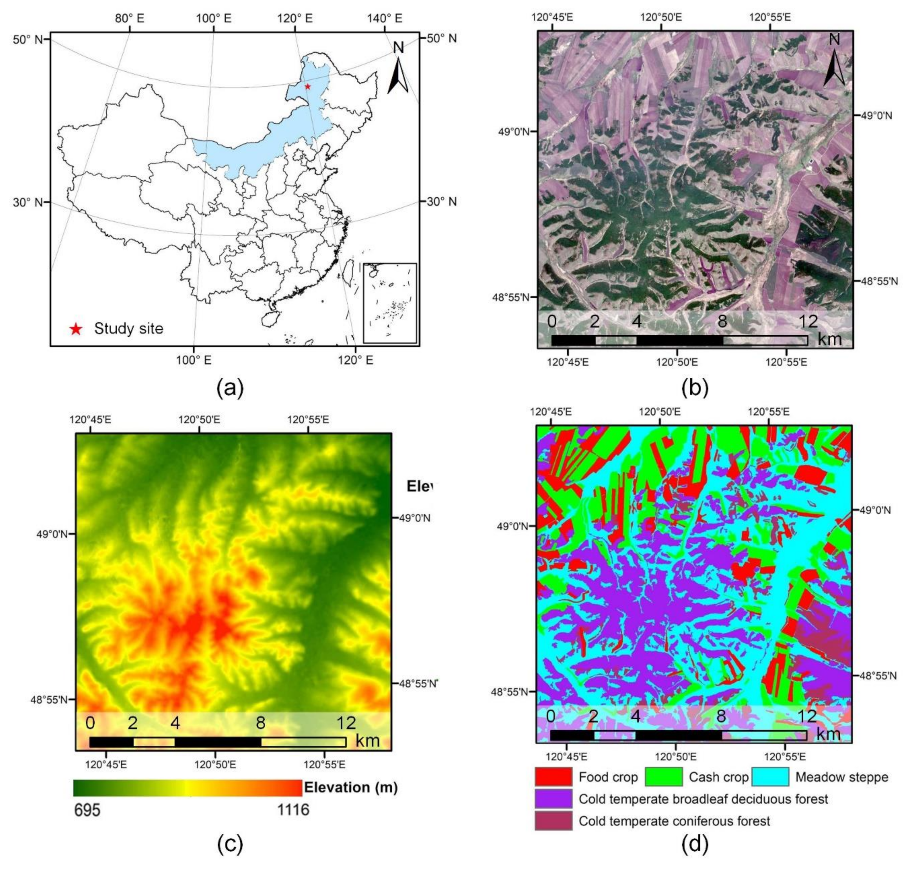
We selected a study area with high vegetation coverage in Tenihe Farm (49°33′N, 120°29′E), which is located in Hulunbuir, Inner Mongolia, China (Figure 2a). This region is characterized by a continental temperate semi-arid climate, with an average annual mean air temperature of −1.8 °C to 2.1 °C and an average annual total precipitation of 350–400 mm [28]. The growing season is from May to September. 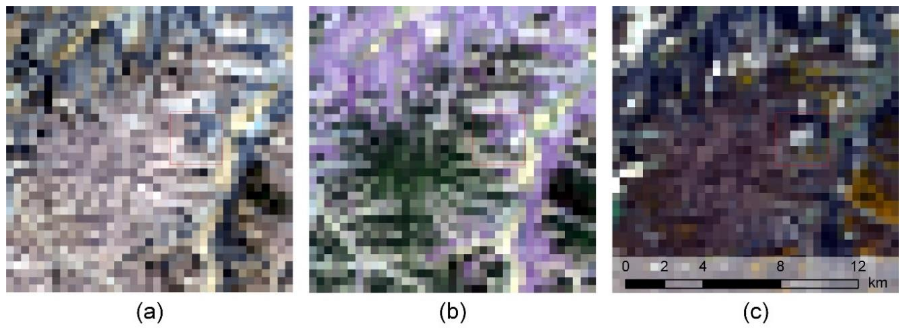For this study we chose a rectangular site of 18 km × 18 km, with UTM coordinates 50 N of the southeast and northwest vertexes (5,421,810, 773,070) and (5,439,810, 791,070), respectively (Figure 2b). The average elevation of the study site is about 850 m and the elevation of the central area is higher than the surrounding (Figure 2c). The study site is in the forest-steppe ecotone with both natural and planted vegetation. Vegetation types in the study area include food crops (e.g., wheat/Triticum aestivum Linn and corn/Zea mays L.), cash crops (e.g., beet/Beta vulgaris Linn., and canola/Brassica campestris L.), meadow steppes (e.g., Chinese leymus/Leymus chinensis (Trin.) and stipa/Stipa capillata Linn.), cold temperate broadleaf deciduous forests (e.g., birch/Betula platyphylla Suk. and aspen/Populus davidiana Dode) and cold temperate coniferous forests (e.g., larch/Larix gmelinii (Ruprecht) Kuzeneva.). Food crops and cash crops are located in the north and south of the study site, meadow steppes and cold temperate broadleaf deciduous forests are distributed in the central area of the study site, and cold temperate coniferous forests are mainly located in the southeastern area of the study site (Figure 2d). The complex and diverse vegetation composition provides an ideal condition for evaluating the performance of the proposed framework in vegetated areas.

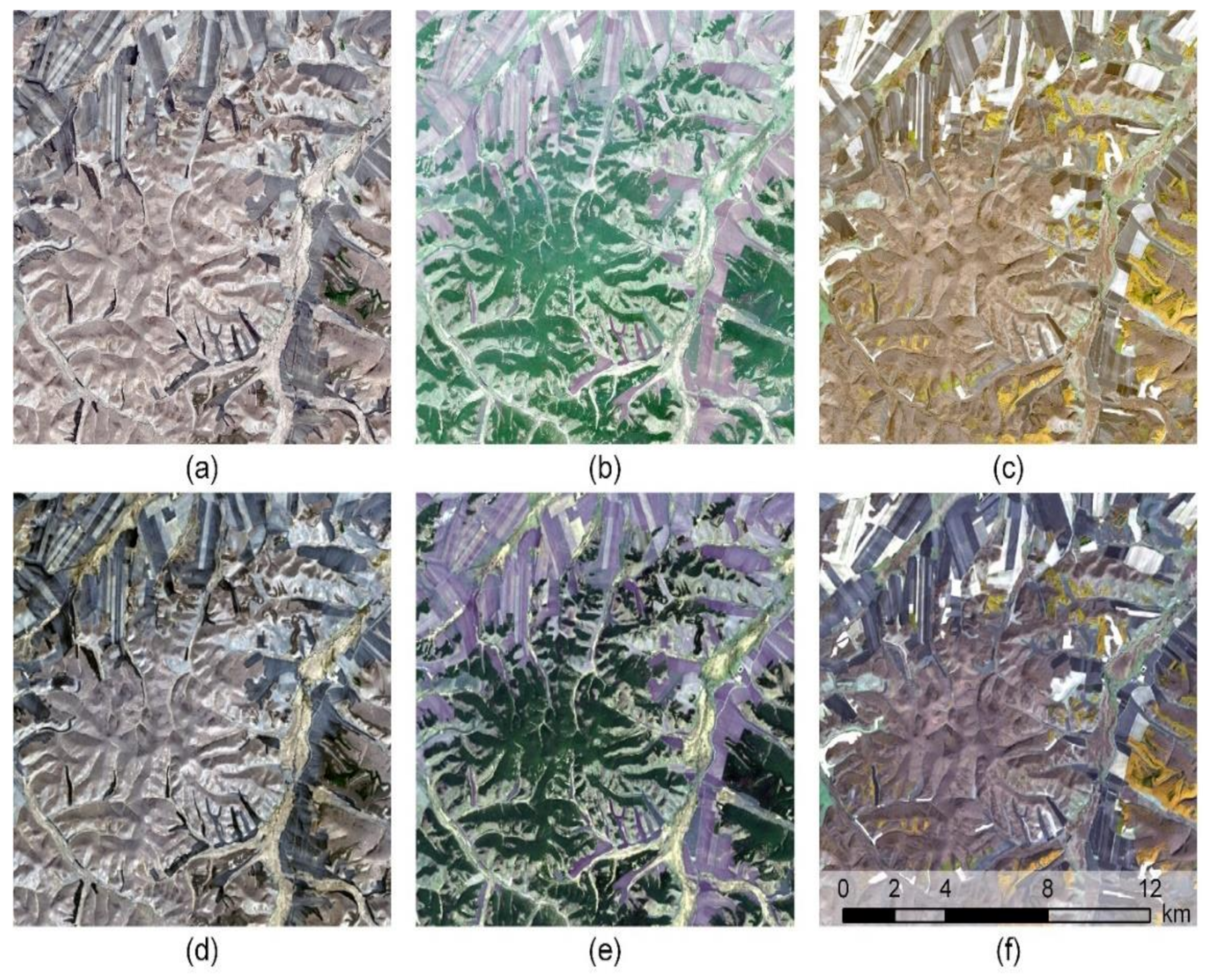
In this study, we used the 10 m resolution Sentinel 2 and 30 m resolution Landsat 8 data. As shown in Figure 3, three sets of cloud-free Sentinel 2 and Landsat 8 images (L1 products) covering the study area were obtained from the Copernicus Open Access Hub (https://scihub.copernicus.eu/) and the United States Geological Survey (USGS) websites (https://earthexplorer.usgs.gov/), respectively. Sentinel 2 images have four 10 m bands (band 2, 3, 4, 8), which were treated as the fine bands to fuse with the corresponding Landsat 8 bands (band 2, 3, 4, 5). Specifically, we employed the cloud-free Sentinel 2 image on 25 April 2018 (Figure 3a) and Landsat 8 images on 24 April 2018 and 26 May 2018 (Figure 3d,e) to predict a Sentinel-like imagery on 26 May 2018 using original and improved STARFM, ESTARFM and FSDAF (

Table 1. Acquisition dates and usages of the collected data. Note that MODIS represents for the Moderate-resolution Imaging Spectroradiometer and N/A represents that the corresponding image is not used in the fusion. The MODIS images here are resampled from Landsat 8.

Acquisition Date	Source	Data Usage
		Sentinel 2-Landsat 8 Fusion	Landsat 8-MODIS Fusion	Sentinel 2-MODIS Fusion
24 April 2018	Landsat 8	Input	Input	N/A
	MODIS	N/A	Input	Input
25 April 2018	Sentinel 2	Input	N/A	Input
26 May 2018	Landsat 8	Input	Reference	N/A
	MODIS	N/A	Input	Input
30 May 2018	Sentinel 2	Reference	N/A	Reference
1 October 2018	Landsat 8	Input	Input	N/A
	MODIS	N/A	Input	Input
2 October 2018	Sentinel-2	Input	N/A	Input

). These images were collected over a one-month timespan in the early growing season of the study site, during which we can clearly observe the vegetation phenological changes (Figure 3). Since the ESTARFM algorithm requires more than one input fine image, we further collected the Sentinel 2 imagery on 2 October 2018 (Figure 3c) and a Landsat 8 imagery on 1 October 2018 (Figure 3f). In October, the study site is at the end of the growing season, and most vegetation has experienced dramatic phenological changes compared with the beginning of the growing season in April.

All collected L1 Sentinel 2 and Landsat 8 data were preprocessed using the Sentinel Application Platform (SNAP) and Land Surface Reflectance Code (LaSRC) to convert to land-surface reflectance products, respectively. Then, all Landsat surface reflectance products were registered to the Sentinel 2 products using the Automated Registration and Orthorectification Package (AROP) [29]. Besides the aforementioned Sentinel 2 and Landsat 8 images, we further simulated a set of 480 m-resolution MODIS images by resampling the Landsat 8 images using the ENVI Software (Figure 4). This is a commonly used method for validating spatiotemporal data-fusion algorithms, because it can avoid the registration errors brought by real images [30]. The eCognition Developer 8.7 software was used to segment objects from the Sentinel 2 image on 25 April 2018 and the Landsat 8 image on 24 April 2018. The segmentation scales were set as the Level 1, Level 2 and Level 3 derived from the ESP 2 tool (with a step size is 1, 3 and 5) respectively. The segmented objects from the Sentinel 2 image were used as the inputs for the fusion between Sentinel 2 and Landsat 8 images and between Sentinel 2 and MODIS images, and those from Landsat 8 images were used as the inputs for the fusion between Landsat 8 and MODIS images.

3.3. Experimental Setup and Accuracy Assessment

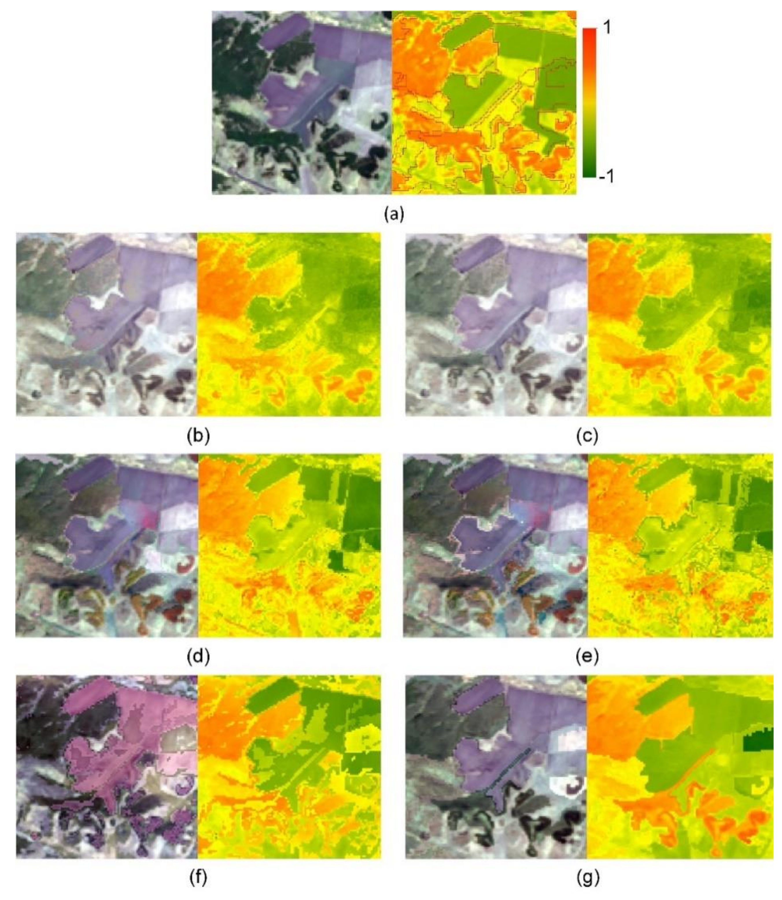
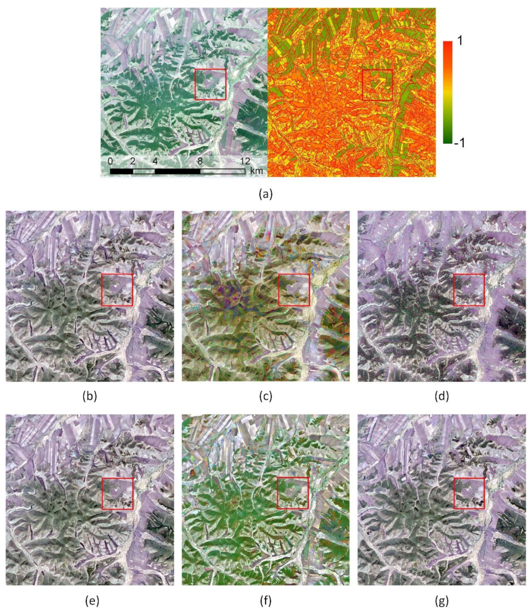
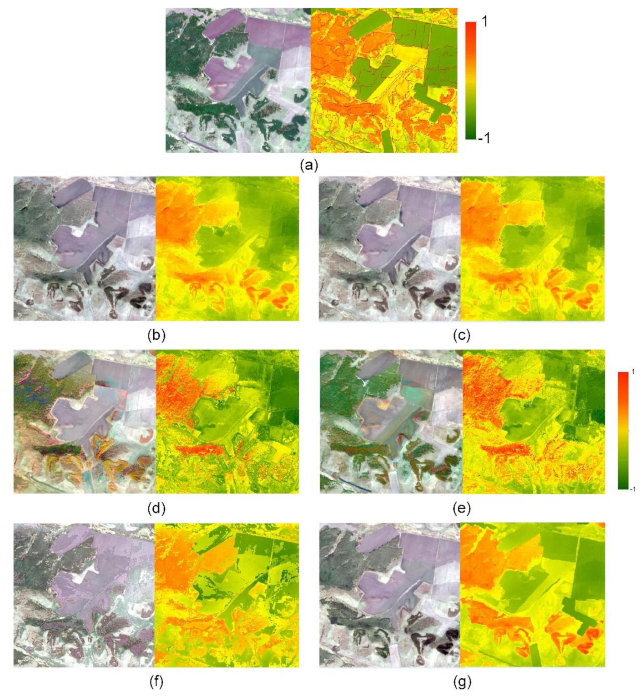
To validate the performance of the proposed framework in the fusion of different dataset combinations, we run the STARFM, ESTARFM, FSDAF, OSTARFM, OESTARFM, and OFSDAF algorithms to fuse the Sentinel 2 data with Landsat 8 data, fuse the Landsat data with MODIS data, and fuse the Sentinel 2 data with MODIS data, respectively. For each data-fusion experiment, the search window size for the similar pixel selection was determined by a trial-and-error method [31]. The window size was set as 4 × n + 1, where n was iteratively increased from 1 to 10 with a step 1. The window size generating the highest fusion accuracy was used to run the corresponding pair of original and object-based spatiotemporal data-fusion algorithms.

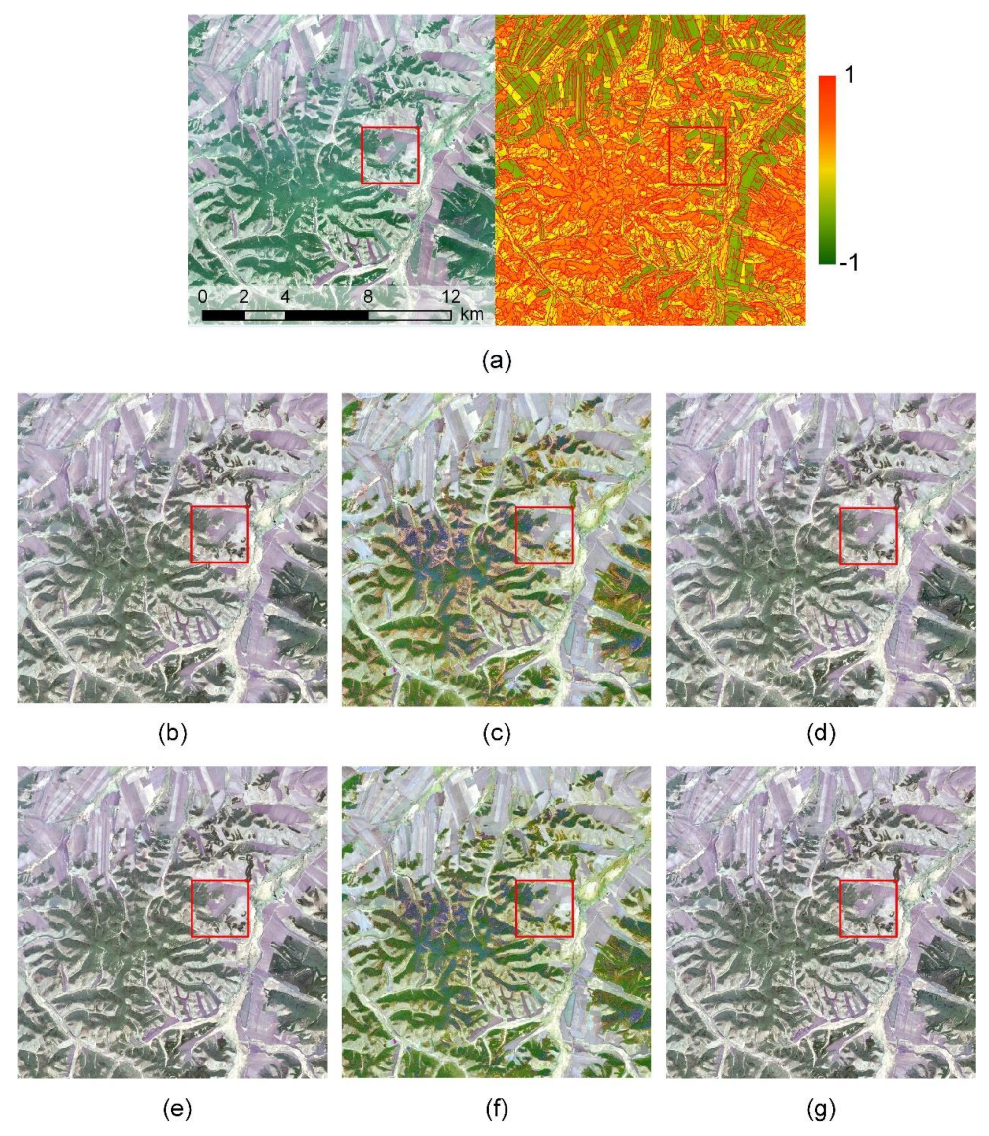
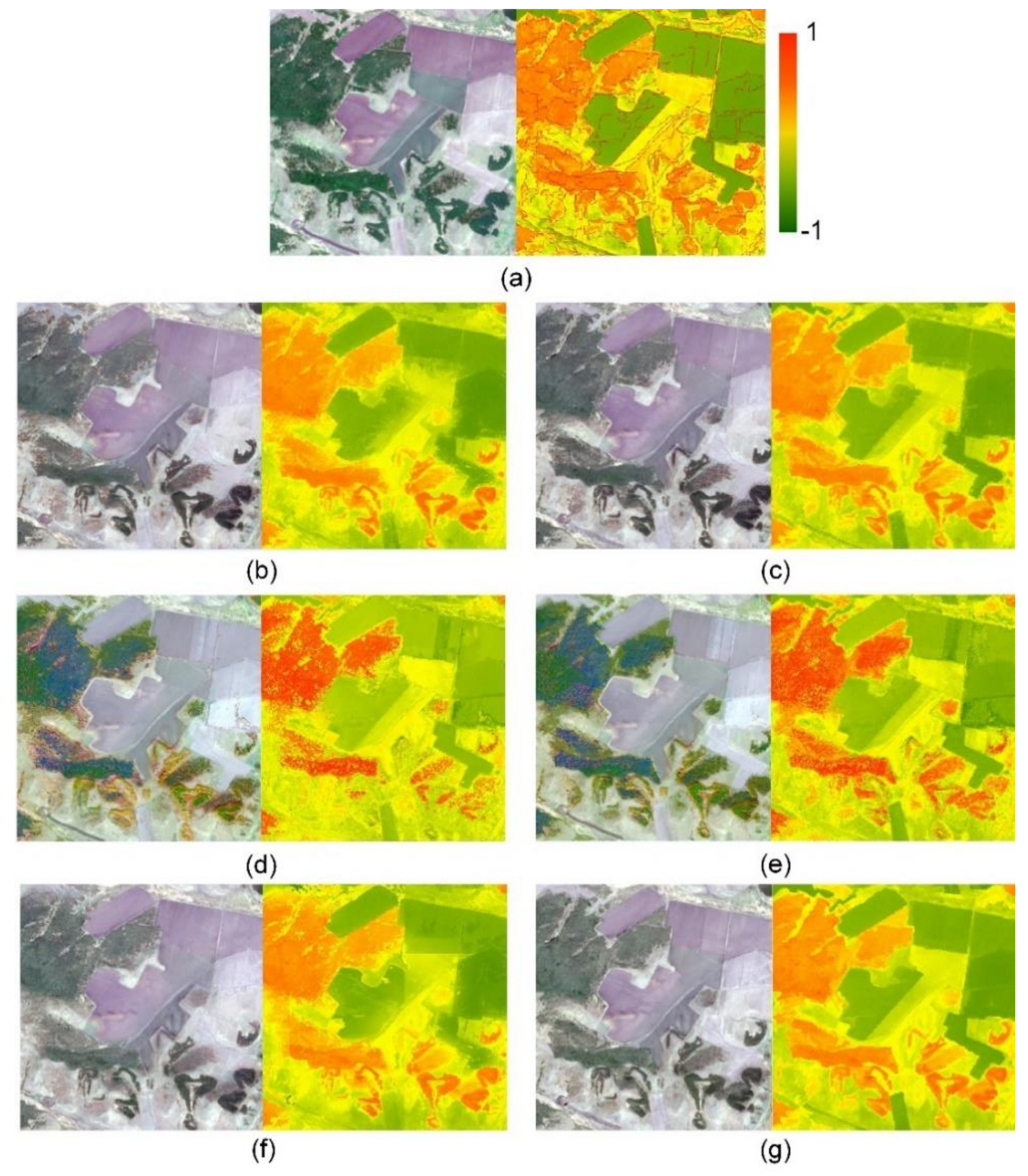
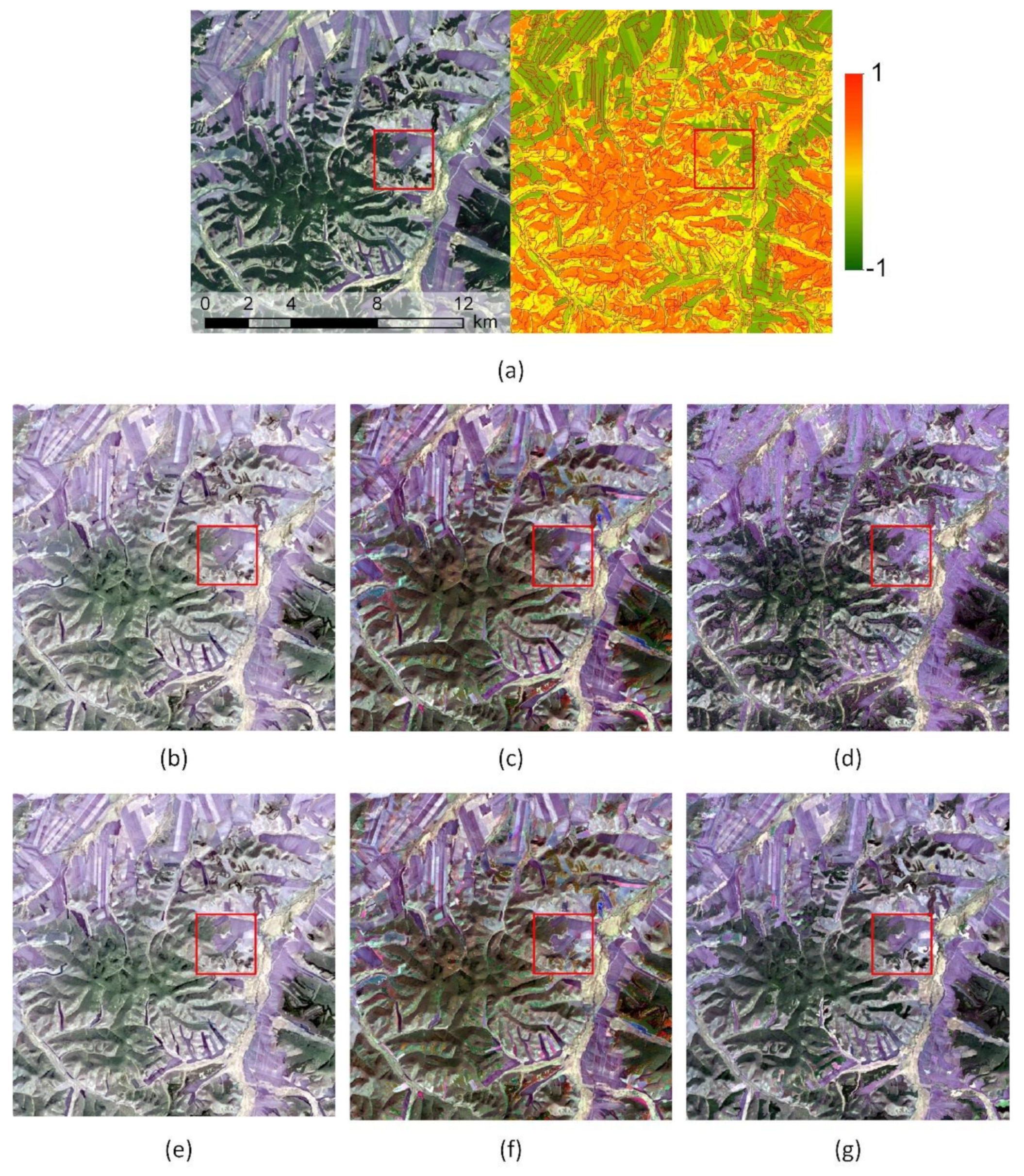
Each predicted image was visually compared to the observed image near the prediction date. Moreover, we calculated four statistics to evaluate quantitatively the fusion accuracy for each individual band (i.e., blue, green, red, and near-infrared/NIR) and normalized difference vegetation index (NDVI), namely the root-mean-square error (RMSE), relative RMSE (rRMSE), average absolute difference (AAD), and Pearson correlation coefficient (r). These four indices have been widely used in the previous studies [13,14]. RMSE and rRMSE provide a global description of the radiometric difference between the predicted imagery and the real reference imagery, AAD is used to measure the average bias for an individual prediction, and r indicates the linear correlation between predicted imagery and the reference imagery. The mathematic definitions of these indices are shown in Equations (2)–(5):

$$RMS{E}_j=\sqrt{\frac{{{\displaystyle \sum }}_{i=1}^N{\left(P_{ij}-Q_{ij}\right)}^2}{N}}$$

(2)

$$rRMS{E}_j=\frac{RMS{E}_j*100}{\overline{Q_j}}$$

(3)

$$r_j=\frac{{{\displaystyle \sum }}_{i=1}^N\left(P_{ij}-\overline{P_j}\right)\left(Q_{ij}-\overline{Q_j}\right)}{\sqrt{{{\displaystyle \sum }}_{i=1}^N{\left(P_{ij}-\overline{P_j}\right)}^2·{{\displaystyle \sum }}_{i=1}^N{\left(Q_{ij}-\overline{Q_j}\right)}^2}}$$

(4)

$$AA{D}_j=\frac{{{\displaystyle \sum }}_{i=1}^N\left|P_{ij}-Q_{ij}\right|}{N}$$

(5)

where N is the total number of pixels, and j indicates the $j\mathrm{th}$ band, and $P_{ij}$ and $Q_{ij}$ are the values of the $i\mathrm{th}$ pixel of $j\mathrm{th}$ band in the predicted imagery and observed reference imagery.

3.4. Vegetation Mapping and Accuracy Assessment

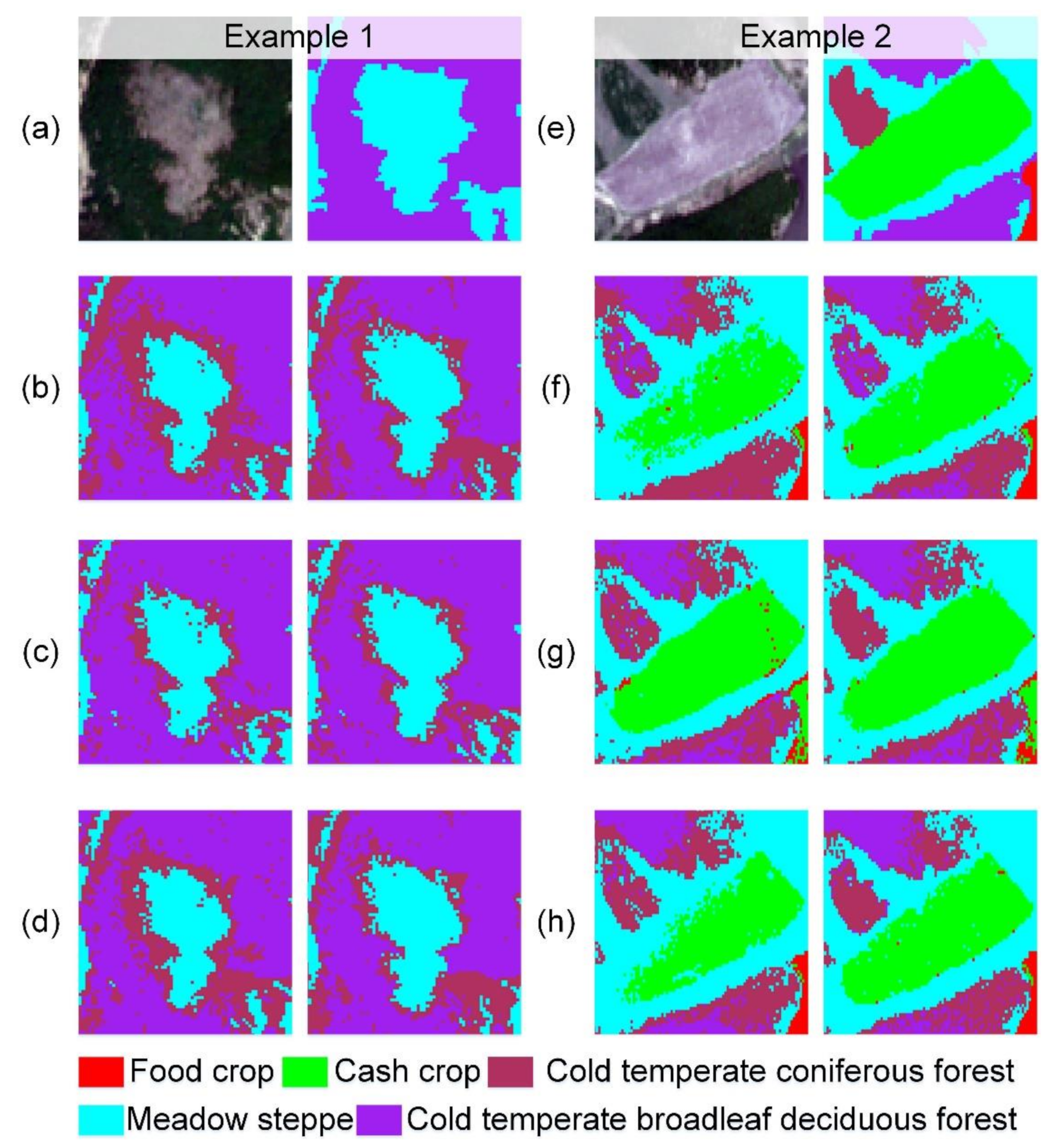
To test the potential of the proposed framework in vegetation mapping, we evaluated the performance differences on vegetation mapping using the fused Sentinel 2 images from both original and modified algorithms. The Support Vector Machine (SVM) algorithm was used to classify the study area into five vegetation types, which are food crops, cash crops, cold temperate coniferous forests, meadow steppes, and cold temperate broadleaf deciduous forests. The original Sentinel 2 image on 25 April 2018 and the fused Sentinel 2 image from Landsat 8 were used as the inputs of SVM classifier. The default SVM classifier with the radial basis function data on 26 May 2018 kernel type in the ENVI software was used here to perform all classifications.

The ground truth of vegetation map was created based on digitalization and validation process. First, we manually digitalized a vegetation map created by the local administration bureau. Then, all polygons within the digitalized map were surveyed in the field to validate its accuracy, and the final vegetation map include 572 polygons with a mean size of 0.623 km². This vector map was then converted to a raster file with a spatial resolution of 10 m. Two thirds of pixels in the ground-truth vegetation map were used as the training samples to train the SVM classifier to generate vegetation maps from the fused images. The remaining one third of pixels were used to evaluate the accuracy of the predicted vegetation maps. Two statistical parameters, i.e., overall accuracy and kappa coefficient, were calculated to assess the accuracy of each predicted vegetation map.

4. Results

4.1. Fusions Between Sentinel 2 and Landsat 8 Images

The three optimized segmentation scales derived from the ESP 2 tool were used for segmenting the Sentinel 2 image on 25 April 2018 are 84, 159 and 159. The same Level 2 and Level 3 optimal scales indicate that the study site displays considerable texture differences. The visual comparison among the three original spatiotemporal data-fusion algorithms shows that all the predicted images on 26 May 2018 have similar spatial patterns on the color ramp as the reference data and can capture the phenological changes of vegetation during the one-month timespan (Figure 5). The STARFM and FSDAF methods show similar fusion results (Figure 5b,d); while the ESTARFM method generates an image with significant color ramp differences (Figure 5c). All three methods generate a large amount of distorted and noisy pixels, especially at the edge between vegetation types, which can be more clearly seen in the NDVI maps (Figure 6b,d,f).

The overall visual patterns of the object-based methods are very close to the fusion results of the original methods (Figure 5). However, all three object-based methods can improve the fusion results by reducing the distortions and noises at the boundaries between vegetation types (Figure 6c,e,g). These visual findings are consistent with the quantitative analysis results. The RMSE, rRMSE and AAD for all three object-based methods decrease for all bands, and the r values all increase (

Table 2. Quantitative assessment of the six spatial and temporal fusion results between Sentinel 2 and Landsat 8 data. Noted that NIR, NDVI, RMSE, rRMSE, AAD and r represent near-infrared, normalized difference vegetation index, root-mean-square error, relative root-mean-square error, average absolute difference and Pearson correlation coefficient, respectively.

		STARFM	OSTARFM	ESTARFM	OESTARFM	FSDAF	OFSDAF
RMSE	B	0.0108	0.0103	0.0183	0.0181	0.0110	0.0108
	G	0.0109	0.0106	0.0165	0.0160	0.0111	0.0114
	R	0.0151	0.0131	0.0219	0.0186	0.0156	0.0143
	NIR	0.0323	0.0273	0.0649	0.0494	0.0326	0.0283
	NDVI	0.0822	0.0678	0.1610	0.1144	0.0899	0.0686
	Mean	0.0303	0.0258	0.0565	0.0433	0.0320	0.0267
rRMSE	B	21.0596	19.9351	35.4933	35.1258	21.4055	20.9133
	G	14.5538	14.1014	21.9743	21.3165	14.7869	15.2283
	R	19.6349	17.0154	28.5337	24.1865	20.3467	18.5621
	NIR	12.6713	10.7312	25.4851	19.3786	12.7864	11.1068
	NDVI	16.1035	13.3362	31.5283	22.4152	17.6032	13.4445
	Mean	16.8046	15.0239	28.6029	24.4845	17.3857	15.8510
r	B	0.8767	0.9029	0.8146	0.8429	0.8696	0.8903
	G	0.8684	0.8879	0.8194	0.8527	0.8586	0.8664
	R	0.8956	0.9270	0.7944	0.8600	0.8848	0.9138
	NIR	0.9133	0.9440	0.7033	0.8000	0.9118	0.9372
	NDVI	0.9445	0.9666	0.7974	0.8884	0.9296	0.9645
	Mean	0.8997	0.9257	0.7858	0.8488	0.8909	0.9144
AAD	B	0.0088	0.0084	0.0150	0.0150	0.0089	0.0087
	G	0.0088	0.0086	0.0134	0.0131	0.0089	0.0091
	R	0.0112	0.0097	0.0157	0.0135	0.0117	0.0107
	NIR	0.0237	0.0201	0.0462	0.0343	0.0241	0.0211
	NDVI	0.0627	0.0517	0.1096	0.0791	0.0679	0.0522
	Mean	0.0230	0.0197	0.0400	0.0310	0.0243	0.0204

). Specifically, the performance of the OSTARFM method is best in the three object-based methods, followed by the OFSDAF method and the OESTARFM method. Moreover, the improvements in the vegetation-related bands (e.g., red, NIR, and NDVI) are greater than in blue and green bands (Table 2). The average improvement of RMSE, rRMSE, r and AAD for the red bands of the three object-based methods are 0.0022, 2.9174%, 0.0420 and 0.0016 which are about 10, 9, 2 and 12 times better (smaller for RMSE, rRMSE and AAD, and larger for r) than the blue and green bands on average; those for the NIR bands of the three object-based methods are 0.0083, 3.2421%, 0.0509 and 0.0062, which are about 39, 10, 2 and 46 times better than the blue and green bands on average; and those for the NDVI bands of the three object-based methods are 0.0274, 5.3464%, 0.0493 and 0.0191, which are about 128, 16, 2 and 143 times better than the blue and green bands on average.

4.2. Fusions Between Landsat 8 and Moderate-Resolution Imaging Spectroradiometer (MODIS) Images

The three optimized segmentation scales derived from the ESP 2 tool for segmenting the Landsat 8 image on 24 April 2018 are 165, 219 and 219, respectively. The three original methods show strong differences in their fusion results, and those from the STARFM are the visually closest to the reference datasets (Figure 7a–d). The results from the ESTARFM method present considerable distortions (Figure 7b) and the results from the FSDAF method show a strong blurring effect at the edges between vegetation types (Figure 7c). In addition, all three methods generate a large amount of distorted and noisy pixels at the edges of different vegetation types (Figure 8b,d,f).

Similar to the fusion results between Sentinel 2 and Landsat 8 images, the object-based methods can improve the spatiotemporal data-fusion results by significantly reducing the distortions and noises and producing clearer vegetation boundaries than the corresponding original method (Figure 8). The RMSE, rRMSE, and AAD have a decrease of 0.0038, 1.6025% and 0.0032 for the three object-based method on average, and the r have an increase of 0.027 on average. The object-based methods have the most significant improving effect in the NIR and NDVI bands and the smallest improving effect on the green bands (

Table 3. Quantitative assessment of the fusion methods for Landsat 8 and Landsat-like MODIS data.

		STARFM	OSTARFM	ESTARFM	OESTARFM	FSDAF	OFSDAF
RMSE	B	0.0077	0.0069	0.0075	0.0075	0.0087	0.0074
	G	0.0078	0.0073	0.0080	0.0079	0.0080	0.0076
	R	0.0155	0.0141	0.0187	0.0196	0.0180	0.0153
	NIR	0.0282	0.0253	0.0498	0.0458	0.0330	0.0273
	NDVI	0.1096	0.0989	0.1332	0.1318	0.1326	0.1071
	Mean	0.0338	0.0305	0.0434	0.0425	0.0401	0.0329
rRMSE	B	18.9576	17.0260	18.4887	18.4586	21.2657	18.1318
	G	11.9878	11.2189	12.2045	12.1021	12.2244	11.6395
	R	22.0662	20.0732	26.7095	27.8927	25.6980	21.8137
	NIR	12.2192	10.9789	21.5547	19.8305	14.3097	11.8348
	NDVI	21.4210	19.3331	26.0284	25.7548	25.9235	20.9332
	Mean	17.3304	15.7260	20.9972	20.8077	19.8843	16.8706
r	B	0.8398	0.8730	0.8484	0.8487	0.7957	0.8586
	G	0.8582	0.8778	0.8472	0.8503	0.8432	0.8650
	R	0.8325	0.8636	0.7441	0.7290	0.7663	0.8412
	NIR	0.8947	0.9160	0.7264	0.7386	0.8600	0.9022
	NDVI	0.8671	0.8925	0.8022	0.8030	0.7960	0.8680
	Mean	0.8585	0.8846	0.7937	0.7939	0.8122	0.8670
AAD	B	0.0059	0.0052	0.0058	0.0057	0.0065	0.0054
	G	0.0059	0.0055	0.0060	0.0059	0.0061	0.0056
	R	0.0121	0.0109	0.0143	0.0147	0.0137	0.0113
	NIR	0.0202	0.0197	0.0375	0.0328	0.0246	0.0204
	NDVI	0.0861	0.0758	0.1028	0.1007	0.0992	0.0782
	Mean	0.0260	0.0234	0.0333	0.0320	0.0300	0.0242

). The average improvement of RMSE, rRMSE and AAD for the NIR and NDVI bands are 0.0080, 1.6465%, and 0.0068 smaller than green bands, and the improvement of average r values are 0.0142 higher. Moreover, comparing with the fusion results between Sentinel 2 and Landsat 8 images, the improving effect of the fusion results in the blue bands between Landsat 8 and MODIS images is much stronger. The average decreases of RMSE, rRMSE and AAD in the Landsat 8-MODIS blue bands are about 2, 3 and 3 times larger than the average decreases in Sentinel 2-Landsat 8 blue bands (Table 2 and Table 3). The Landsat 8-MODIS red band from the OESTARFM method is the only band showing no improving effect compared with the original method (Table 2).

4.3. Fusions Between Sentinel 2 and MODIS Images

The same objects derived from the Sentinel 2 image on 25 April 2018 are used here for the fusion between Sentinel 2 and MODIS images. By visually comparing with the reference map in Figure 9a, we can see that the Sentinel 2-MODIS fusion results are not as good as the Sentinel 2-Landsat 8 fusion results (Figure 9b–d). All three results from original methods look distorted compared to the reference image, with the most severe distortion results from the ESTARFM method (Figure 9c). Moreover, all three results from original methods have a large amount of noise at the boundaries between vegetation types (Figure 10b,d,f). The improvements of the object-based methods for the Sentinel 2-MODIS fusion become less stable. The overall color ramps for the fusion results of the OSTARFM and the OFSDAF methods look very similar to the original maps, except for the color ramp for the results of OESTARFM result (Figure 9e–g). The OFSDAF method performs the best in noise reduction and defines the vegetation type boundaries more clearly (Figure 10g).

The quantitative assessments also confirm the above results. As can be seen from

Table 4. Quantitative assessment of the fusion methods for Sentinel 2 and Landsat-like MODIS data.

		STARFM	OSTARFM	ESTARFM	OESTARFM	FSDAF	OFSDAF
RMSE	B	0.0125	0.0126	0.0205	0.0207	0.0131	0.0119
	G	0.0128	0.0129	0.0174	0.0176	0.0124	0.0125
	R	0.0201	0.0201	0.0269	0.0268	0.0223	0.0177
	NIR	0.0416	0.0414	0.0765	0.0707	0.0441	0.0389
	NDVI	0.1215	0.1217	0.1898	0.1630	0.1483	0.0994
	Mean	0.0417	0.0417	0.0662	0.0598	0.0480	0.0361
rRMSE	B	24.2959	24.3215	39.6935	40.0359	25.3375	23.0448
	G	17.0554	17.1338	23.1439	23.4031	16.5104	16.5717
	R	26.0844	26.1027	34.9109	34.8233	28.9996	22.9375
	NIR	16.3927	16.2887	30.1336	27.8528	17.3534	15.3110
	NDVI	23.9152	23.9491	37.3573	32.689	29.1889	19.5576
	Mean	21.5487	21.5592	33.0478	31.7608	23.4780	19.4845
r	B	0.7950	0.7970	0.7360	0.7294	0.7660	0.8380
	G	0.8000	0.8006	0.7365	0.7313	0.7801	0.8184
	R	0.7930	0.7945	0.6191	0.6313	0.7421	0.8527
	NIR	0.8369	0.8392	0.5349	0.6089	0.8140	0.8638
	NDVI	0.8549	0.8525	0.6364	0.7228	0.7813	0.9063
	Mean	0.8160	0.8168	0.6526	0.6847	0.7767	0.8558
AAD	B	0.0100	0.0100	0.0170	0.0171	0.0103	0.0094
	G	0.0101	0.0101	0.0141	0.0142	0.0097	0.0097
	R	0.0159	0.0158	0.0205	0.0202	0.0176	0.0133
	NIR	0.0322	0.0320	0.0585	0.0502	0.0338	0.0295
	NDVI	0.0966	0.0957	0.1459	0.1250	0.1162	0.0764
	Mean	0.0330	0.0327	0.0512	0.0453	0.0375	0.0277

, the average RMSE, rRMSE and AAD are the largest among the three experimental results, and the average r values are the lowest. Moreover, the OSTARFM method shows no significant improvements in all bands. Its RMSE, rRMSE, r and AAD vales are almost the same as the STARFM method (Table 4). The OESTARFM method has no significant improvements in the blue, green, and red bands as well (Table 4). Although it has a 2.2868% improvement in rRMSE in the NIR and NDVI bands on average, their RMSE, rRMSE and AAD values are still the largest among all three object-based methods (Table 4). The OFSDAF method is the only object-based method that can still significantly improve the fusion results in the blue, red and NIR and NDVI bands. It has a decrease of 0.0012, 0.0046, 0.0052, and 0.0489 in RMSE in the blue, red, NIR and NDVI bands, respectively, which are also the smallest among all three object-based methods.

4.4. Results of Vegetation Mapping

Table 4 reports the statistical results of the vegetation classification results using the fused images from both object-based methods and original methods. Although the STARFM outperformed the ESTARFM and FSDAF methods in the fusion of Sentinel 2 and Landsat 8 images (Table 2), the classification of the STARFM fused image shows the lowest accuracy. Overall, the classification accuracy of the fused images from original fusion methods do not show correlation with their fusion accuracy.

As for the classification results of the fused images from object-based fusion methods, the visual differences between them and those from original fusion methods are not obvious (Figure A1), but their overall accuracy and kappa coefficient are all increased by 2% (

Table 5. Accuracy assessment of the vegetation mapping results.

	STARFM	OSTARFM	ESTARFM	OESTARFM	FSDAF	OFSDAF
Overall accuracy	0.68	0.70	0.71	0.73	0.69	0.71
Kappa coefficient	0.59	0.61	0.62	0.64	0.60	0.62

and

Table A1. Confusion matrix of the vegetation mapping results using the fused images from the STARFM algorithm.

	Food Crop	Cash Crop	Meadow Steppe	Cold Temperate Coniferous Forest	Cold Temperate Broadleaf Deciduous Forest	User Accuracy
Food crop	0.64	0.36	0.03	<0.01	<0.01	0.51
Cash crop	0.18	0.57	0.02	<0.01	<0.01	0.78
Meadow steppe	0.17	0.06	0.84	0.13	0.07	0.83
Cold temperate coniferous forest	<0.01	<0.01	0.11	0.63	0.34	0.21
Cold temperate broadleaf deciduous forest	<0.01	<0.01	0.01	0.23	0.58	0.90
Producer accuracy	0.64	0.57	0.84	0.63	0.58
Overall accuracy	0.68
Kappa coefficient	0.59

,

Table A2. Confusion matrix of the vegetation mapping results using the fused images from the OSTARFM algorithm.

	Food Crop	Cash Crop	Meadow Steppe	Cold temperate Coniferous Forest	Cold temperate Broadleaf Deciduous Forest	User Accuracy
Food crop	0.64	0.35	0.03	<0.01	<0.01	0.51
Cash crop	0.18	0.59	0.01	<0.01	<0.01	0.79
Meadow steppe	0.18	0.05	0.85	0.11	0.07	0.84
Cold temperate coniferous forest	<0.01	<0.01	0.10	0.67	0.30	0.24
Cold temperate broadleaf deciduous forest	<0.01	<0.01	0.01	0.22	0.62	0.91
Producer accuracy	0.64	0.59	0.85	0.67	0.62
Overall accuracy	0.70
Kappa coefficient	0.61

,

Table A3. Confusion matrix of the vegetation mapping results using the fused images from the ESTARFM algorithm.

	Food Crop	Cash Crop	Meadow Steppe	Cold Temperate Coniferous Forest	Cold Temperate Broadleaf Deciduous Forest	User Accuracy
Food crop	0.57	0.33	0.03	<0.01	<0.01	0.49
Cash crop	0.24	0.63	0.02	<0.01	<0.01	0.75
Meadow steppe	0.19	0.04	0.83	0.10	0.08	0.84
Cold temperate coniferous forest	<0.01	<0.01	0.09	0.64	0.25	0.26
Cold temperate broadleaf deciduous forest	<0.01	<0.01	0.02	0.25	0.67	0.90
Producer accuracy	0.57	0.63	0.83	0.64	0.67
Overall accuracy	0.71
Kappa coefficient	0.62

,

Table A4. Confusion matrix of the vegetation mapping results using the fused images from the OESTARFM algorithm.

	Food Crop	Cash Crop	Meadow Steppe	Cold Temperate Coniferous Forest	Cold Temperate Broadleaf Deciduous Forest	User Accuracy
Food crop	0.61	0.31	0.03	<0.01	<0.01	0.53
Cash crop	0.22	0.65	0.02	<0.01	<0.01	0.77
Meadow steppe	0.17	0.04	0.85	0.12	0.08	0.84
Cold temperate coniferous forest	<0.01	<0.01	0.09	0.64	0.22	0.27
Cold temperate broadleaf deciduous forest	<0.01	<0.01	0.02	0.24	0.69	0.91
Producer accuracy	0.61	0.65	0.85	0.64	0.69
Overall accuracy	0.73
Kappa coefficient	0.64

,

Table A5. Confusion matrix of the vegetation mapping results using the fused images from the FSDAF algorithm.

	Food Crop	Cash Crop	Meadow Steppe	Cold Temperate Coniferous Forest	Cold Temperate Broadleaf Deciduous Forest	User Accuracy
Food crop	0.64	0.37	0.03	<0.01	<0.01	0.50
Cash crop	0.18	0.57	0.02	<0.01	<0.01	0.79
Meadow steppe	0.18	0.06	0.84	0.12	0.08	0.83
Cold temperate coniferous forest	<0.01	<0.01	0.10	0.61	0.29	0.22
Cold temperate broadleaf deciduous forest	<0.01	<0.01	0.02	0.27	0.63	0.90
Producer accuracy	0.64	0.57	0.84	0.61	0.63
Overall accuracy	0.69
Kappa coefficient	0.60

and

Table A6. Confusion matrix of the vegetation mapping results using the fused images from the OFSDAF algorithm.

	Food Crop	Cash Crop	Meadow Steppe	Cold Temperate Coniferous Forest	Cold Temperate Broadleaf Deciduous Forest	User Accuracy
Food crop	0.64	0.35	0.02	<0.01	<0.01	0.52
Cash crop	0.18	0.60	0.01	<0.01	<0.01	0.80
Meadow steppe	0.17	0.04	0.86	0.10	0.07	0.85
Cold temperate coniferous forest	<0.01	<0.01	0.10	0.63	0.28	0.23
Cold temperate broadleaf deciduous forest	<0.01	<0.01	0.01	0.27	0.64	0.90
Producer accuracy	0.64	0.60	0.86	0.63	0.64
Overall accuracy	0.71
Kappa coefficient	0.62

). After zooming in, the visual inspection results show that the vegetation maps using images from the object-based fusion algorithms have less “pepper-salt” effect (Figure 11). The misclassified cold temperate coniferous forest close to the boundary of meadow-steppe in Figure 11a–d can be reduced by using the object-based framework, and the cash crop boundary in Figure 11e–h is closer to the real boundary by using the object-based framework.

5. Discussion

5.1. Improvements of the Proposed Object-Based Data-Fusion Framework

Generation of unified high-resolution time-series images from different remote-sensing sensors can provide support for vegetation mapping and monitoring [32,33]. However, the high spectral similarity in the reflectance spectrum of different vegetation types may bring many misidentified similar pixels, which can disturb spectrum property of vegetation in fused images and thereby cause uncertainties in subsequent applications.

This demonstrates that the proposed framework shows the potential to improve the similar pixel selection results in areas with high spectral similarity. By taking texture information into the similar pixel selection, the reflectance spectral value is not the only parameter in determining similar pixels of a target pixel. With the help of texture information, each segmented object can be treated as a homogenous vegetation patch [34], which can help reduce wrong similar pixels with similar spectral characteristics but different vegetation types. Therefore, the object-based fusion framework can delineate the boundaries between vegetation types more clearly and reduce the “pepper-salt” effect of the original algorithms (Figure 6, Figure 8 and Figure 10).

The object-based spatiotemporal data-fusion framework can be adapted to various vegetated areas under different vegetation covers. Regardless of whether there are significant spectral differences among vegetation types, the proposed method is always beneficial to improve the fusion accuracy. For areas with high inter-vegetation spectral differences, although the spectrum-based similar pixel selection can obtain accurate similar pixels in the interior of each vegetation areas, boundaries between vegetation types might be changed after the spatiotemporal fusion because of the mixed pixels in the junction areas of different vegetation types. In that case, delineated boundaries between vegetation types can ensure the consistency of vegetation types before and after fusion (Figure 6, Figure 8 and Figure 10).

The object-based constraint can further increase the homogeneity within similar pixels to improve the fusion accuracy. In medium NDVI areas, which are mixed with grasslands and forests in this study, three modified algorithms perform better than their original algorithms (Figure 12). As for areas with similar spectral vegetation, the proposed object-based framework can use the texture and shape information to differentiate vegetation types to reduce the wrong similar pixels. For example, the low NDVI areas in this study are mainly composed of grasslands and croplands, which are all covered by bare soil at the acquisition time of the input fine imagery (Figure 3a). Since croplands usually have a regular shape with distinct boundaries [35], the proposed object-based framework have well identified boundaries between grasslands and croplands from a single imagery and, therefore, increase the similar pixel selection accuracy.

Except for texture information, some spatiotemporal fusion methods use temporal changes to address the high spectral similarity problem in similar pixel selection [36]. This strategy has been adopted in the ESTARFM algorithm, which uses two input fine images to select the similar pixels. Taking low NDVI areas in this study as an example, phenological changes between grasslands and croplands can ensure the high accuracy of the similar pixel selection through the ESTARFM algorithm [37], which might be the reason of why the modified ESTARFM has smaller improvements than the modified STARFM and FSDAF. However, temporal changes might not be useful in areas with similar phenological changes but different vegetation types such as the high NDVI areas in this study, which are covered by broadleaf deciduous forests and coniferous forests. The broadleaf deciduous forests are composed of birch trees and aspen trees that have similar phenological changes in the timespan between the input image date and targeted data-fusion date, and the coniferous forests have smaller phenological changes [38]. The similar or small phenological changes might reduce the effectiveness of similar pixel selection using multiple input fine images. Moreover, the long timespan between the targeted data-fusion date and posterior input image date might bring nonlinear phenological changes and, therefore, lead to larger uncertainties in the ESTARFM fused results [39,40]. Under these circumstances, the proposed framework is still effective to improve the data-fusion results of the ESTARFM algorithm.

In addition, vegetation spectral characteristics in different bands can also lead the performance of the proposed framework on bands sensitive to vegetation information (e.g., NIR band) to be better than on other bands (e.g., blue band). This might be mainly because the reflectance differences in vegetation sensitive bands are greater than in other bands due to the control of chlorophyll [41]. Moreover, the bandwidth differences in the red and NIR bands are generally larger than in the blue and green bands [42], and this can cause larger reflective differences in vegetation-sensitive bands as well. For example, the absolute bandwidth difference in the near-infrared band between Sentinel 2 and Landsat 8 images is around 5 and 3 times larger than those in the blue and green bands. Large reflectance differences can make the selection of similar pixels more challenging [43]. The proposed object-based framework can effectively reduce the wrong similar pixel selection by using texture information and, therefore, improve the fusion results of vegetation-sensitive bands.

5.2. Sensitivity of the Proposed Object-Based Framework

The proposed framework can be applied to any spatiotemporal data-fusion algorithm based on similar pixels. Since the proposed framework is implemented based on the principle of the original algorithm by revising the similar pixel selection procedure, the accuracy of the revised object-based method is greatly influenced by the original method. Overall, in this study, the OSTARFM method outperformed the OESTARFM and OFSDAF methods, which is generally consistent with the original methods but with improvements. The improvements on the ESTARFM and FSDAF methods are more obvious than on the STARFM method across different sensor combinations. The different improvements of these three modified algorithms might be related to the differences in the principle of how the similar pixels are used to predict the value of a fused pixel. Most of the spatiotemporal data-fusion algorithms has two components in the final prediction of a fused pixel, i.e., the temporal change predicted from the coarse pixel and the weighted prediction value from similar pixels [9]. In the STARFM method, the temporal change calculated from a coarse pixel is directly added to the predicted fine pixel within it without using the similar pixels. On the other hand, the ESTARFM method uses the similar pixels to calculate a linear conversion coefficient to predict the temporal change from the coarse pixel [12]. Therefore, the highly accurate similar pixels provided by the proposed framework may result in greater improvements on the ESTARFM method. As for the FSDAF method, it calculates the temporal change of a predicting fine pixel by assuming that the temporal change of the corresponding coarse pixel can be distributed to the fine pixels within it based on an auxiliary classification map [14]. In this study, we replaced the classification map with the segmented objects and treated them as the local vegetation units. It has been shown that segmented objects might reflect the vegetation units at a local scale more accurately than an unsupervised pixel-based classification map [44], which therefore might help to increase the fusion accuracy. Due to the influence of similar pixels on the fusion procedure vary in spatiotemporal data-fusion algorithms, it should be mentioned the current study does not focus on the comparisons of different spatiotemporal fusion algorithms, but evaluates their improvements when incorporating an object-based framework. The performance of the object-based methods may vary with different land-surface types and data inputs [45,46].

In addition to the principle of original algorithms, the resolution difference between the input fine and coarse images is another factor that may influence the performance of the proposed framework. The Sentinel 2-Landsat 8 combination has less resolution difference than Sentinel 2-MODIS combination. As can be seen from Table 3 and Table 5, the performance of the object-based methods decreases with the increase in resolution difference. The larger unmixing uncertainty in the fusion of two sensors with the large resolution differences might be the main reason leading to this phenomenon [47]. However, one exception to this trend is the OFSDAF method, this might be caused by the fact that the FSDAF algorithm has better ability to unmix the mixed pixel than STARFM and ESTARFM algorithms.

The proposed object-based framework shows smaller sensitivity to the resolution differences in all three tested algorithms. Here, we used the FSDAF method as an example to evaluate the sensitivity of the proposed object-based method with different resolution combinations, because the FSDAF method showed the largest variations in the three experiments of this study (Table 3, Table 4 and Table 5). As shown in Figure 13, the Sentinel 2 images were used as the fine image, and coarse images with different resolutions were simulated by interpolating the Landsat 8 images using a similar method of generating MODIS images. Overall, the rRMSE of the OFSDAF is much smaller than FSDAF across all resolution combinations, and its increase in rRMSE from a resolution ratio of 5 to 50 is around 4%, which is much smaller than that of the FSDAF (around 10%) (Figure 13). Nevertheless, we still suggest that choosing two sensors with smaller differences in spatial resolutions might be beneficial for spatiotemporal data fusion using the object-based framework.

The scale of segmentation is also critical to the performance of the proposed framework, especially the baseline segmentation scale. The baseline segmentation scale determined the minimum size of the objects and thereby decided the quantity and homogeneity of the similar pixels. Under the same baseline segmentation scale, a bigger search window size might also result in more similar pixels with less with the changes of baseline scale and search window size (Figure 14a,c). With the increase of the homogeneity. Here, we evaluated the performance of the three object-based methods with variations in the baseline scale and search window size (Figure 14). In general, the OSTARFM and OFSDAF methods showed the same pattern in accuracy baseline segmentation scale and search window size, the accuracy of the OSTARFM and OFSDAF decreases significantly. This might be caused by the “restrict-and-select” similar pixel selection approach used by these two methods, which aims to find N similar pixels with the smallest spectral distance. The heterogeneity among pixels decreased with the increase of the baseline segmentation scale and search window size, and the matter of “same spectral from different materials” may lead the selected similar pixels from the OSTARFM and OFSDAF method to have larger heterogeneity from different vegetation types, which therefore reduces the data-fusion accuracy. The accuracy of the OESTARFM method has an opposite changing trend with the variations of baseline segmentation scale and search window size (Figure 14b). This might be caused by the fact that the number of similar pixels becomes insufficient with the reduction of the baseline segmentation scale and search window size. The OESTARFM method adopts a much tighter rule to select similar pixels than the OSTARFM and OFSDAF method. The spectral distance between the similar pixel and targeted pixel should be smaller than the thresholds determined by the standard deviation of each band, and only the common similar pixels selected from the two input fine images are retained [12]. The decreases in baseline segmentation scale and search window size can further reduce the number of selected similar pixels and lead to low data-fusion accuracy. Therefore, we suggest that the combination of baseline segmentation scale and search window size should be determined based on the similar pixel strategy of the original data-fusion algorithm. If the original method uses a loose “restrict-and-select” approach, the baseline segmentation scale and search window size should be relatively small to find similar pixels with heterogeneous vegetation types; if the original method uses a tight “select-and-restrict” approach, they should be set large enough to find a sufficient number of similar pixels.

5.3. Influences on Vegetation Mapping

Times-series high-resolution remote sensing images are beneficial for vegetation mapping [48]. The proposed object-based framework can increase the accuracy of spatiotemporal data fusion, which should be able to improve the vegetation mapping accuracy. In this study, the overall accuracy of the vegetation classification results using the fused images from the object-based methods showed a ~2% improvement than that from the original methods (Table 4) and showed less “pepper-salt” effect at the boundaries between vegetation types (Figure 11). The clearer vegetation boundary and shape preserved in the time-series images from the object-based fusion framework can help better identifying the boundaries between vegetation types.

However, the vegetation classification accuracy in the present study is still relatively low, and the results using the fused images from the object-based framework cannot largely resolve the misclassification issue. This might be caused by two factors. First, this study only used images from two time stamps, and one of the images was in the early growing season without strong vegetation signals. Moreover, this study simply used the SVM algorithm without tuning its parameters. If the spectral differences among vegetation types become larger or the capability of the classifier is improved, the spatiotemporal data-fusion results might have a greater impact on vegetation mapping [49].

5.4. Limitations of the Current Study

Overall, the proposed object-based spatiotemporal data-fusion framework shows great potential to increase the spatiotemporal data-fusion accuracy in vegetated areas by improving the similar pixel selection results. Although the increase in accuracy is limited, it is comparable to other similar spatiotemporal data-fusion works [25,50]. More importantly, the proposed framework can greatly help to preserve vegetation boundary and shape, which therefore can significantly reduce the “pepper-salt” effect in vegetation mapping.

However, there are still limitations that need to be further studied. First, the present study only evaluates the improvements of the proposed framework on the STARFM, ESTARFM and FSDAF methods with a limited number of vegetation types (e.g., grasslands, coniferous forests, broadleaf forests, meadow steppes, and croplands) under three senor combinations. The applicability of the proposed object-based data-fusion framework on different spatiotemporal data-fusion algorithms with more remote sensing datasets needs to be further studied. A more complete evaluation can provide guidance on how to choose the appropriate spatiotemporal data-fusion algorithm to be incorporated with the proposed object-based framework. Second, the proposed framework may result in an insufficient number of similar pixels for the methods using tight rules for similar pixel selection. The strategy of how to coordinate the segmentations scale with the search window size to ensure a sufficient number of similar pixels with high quality still needs to be further studied. Third, the present study only evaluates influence of the proposed framework on vegetation mapping using images from two time stamps and using a simple SVM classifier. Further studies are still needed to evaluate whether the vegetation mapping accuracy can be further improved by including more time-series high-resolution images and using more advanced machine learning classifiers (such as deep learning) [51]. Last but not least, the proposed object-based framework only used segmented objects to improve the similar pixel selection results. Some spectral measure methods such as spectral angle measure [52] and spectral correlation measure [53] also can be used to find the similarity among the pixels. How to integrate the present object-based framework with these spectral measure methods to better improve the fusion accuracy needs to be further studied.

6. Conclusions

This study proposed a general object-based spatiotemporal data-fusion framework to improve the data-fusion accuracy in complex vegetated areas. It can be based on any spatiotemporal data-fusion algorithms by replacing their original similar pixel selection method with an object-restricted method. Here, we modified the STARFM, ESTARFM and FSDAF algorithms to evaluate the performance of the proposed framework. The results show that the object-based framework can improve the performance of all three methods by significantly reducing the “salt and pepper” effect in the fusion result and delineating the vegetation boundaries more clearly. Overall, the three object-based methods perform the best in the fusion of Sentinel-2 and Landsat images. The improvements in the vegetation-sensitive bands (e.g., red and NIR bands) are stronger than in other bands (e.g., blue and green bands). The baseline segmentation scale and the search window size are the two major factors influencing the performance of an object-based spatiotemporal data-fusion algorithm, and users should select the optimal values based on the similar pixel selection method. If an algorithm adopts a loose “select-and-restrict” similar pixel selection strategy, a relatively small baseline segmentation scale and search windows size should be used; if an algorithm adopts a tight “restrict-and-select” strategy, a relatively large baseline segmentation scale and search windows size should be used. Overall, the proposed object-based framework shows great potential for generating time series of remote-sensing images with high spatial resolutions in complex vegetated areas and, therefore, provides useful data sources for mapping vegetation attributes and monitoring vegetation changes accurately.

References

1. Xie, Y.; Sha, Z.; Yu, M. Remote sensing imagery in vegetation mapping: A review. J. Plant Ecol. 2008, 1, 9–23. [Google Scholar] [CrossRef]
2. Mehner, H.; Cutler, M.; Fairbairn, D.; Thompson, G. Remote sensing of upland vegetation: The potential of high spatial resolution satellite sensors. Glob. Ecol. Biogeogr. 2004, 13, 359–369. [Google Scholar] [CrossRef]
3. Townsend, P.A.; Walsh, S.J. Remote sensing of forested wetlands: Application of multitemporal and multispectral satellite imagery to determine plant community composition and structure in southeastern USA. Plant Ecol. 2001, 157, 129–149. [Google Scholar] [CrossRef]
4. Marcinkowska-Ochtyra, A.; Zagajewski, B.; Raczko, E.; Ochtyra, A.; Jarocińska, A. Classification of High-Mountain Vegetation Communities within a Diverse Giant Mountains Ecosystem Using Airborne APEX Hyperspectral Imagery. Remote Sens. 2018, 10, 570. [Google Scholar] [CrossRef] [Green Version]
5. Qader, S.H.; Dash, J.; Atkinson, P.M.; Rodriguez-Galiano, V. Classification of vegetation type in Iraq using satellite-based phenological parameters. IEEE J. Sel. Top. Appl. Earth Obs. Remote Sens. 2016, 9, 414–424. [Google Scholar] [CrossRef]
6. Yan, J.; Zhou, W.; Han, L.; Qian, Y. Mapping vegetation functional types in urban areas with WorldView-2 imagery: Integrating object-based classification with phenology. Urban For. Urban Green. 2018, 31, 230–240. [Google Scholar] [CrossRef]
7. Price, J.C. How unique are spectral signatures? Remote Sens. Environ. 1994, 49, 181–186. [Google Scholar] [CrossRef]
8. Zhang, Y.; Wen, F.; Gao, Z.; Ling, X. A Coarse-to-Fine Framework for Cloud Removal in Remote Sensing Image Sequence. IEEE Trans. Geosci. Remote Sens. 2019, 57, 5963–5974. [Google Scholar] [CrossRef]
9. Chen, B.; Huang, B.; Xu, B. Comparison of spatiotemporal fusion models: A review. Remote Sens. 2015, 7, 1798–1835. [Google Scholar] [CrossRef] [Green Version]
10. Li, X.; Ling, F.; Foody, G.M.; Ge, Y.; Zhang, Y.; Du, Y. Generating a series of fine spatial and temporal resolution land cover maps by fusing coarse spatial resolution remotely sensed images and fine spatial resolution land cover maps. Remote Sens. Environ. 2017, 196, 293–311. [Google Scholar] [CrossRef]
11. Zhu, X.; Cai, F.; Tian, J.; Williams, T. Spatiotemporal fusion of multisource remote sensing data: Literature survey, taxonomy, principles, applications, and future directions. Remote Sens. 2018, 10, 527. [Google Scholar]
12. Zhu, X.; Chen, J.; Gao, F.; Chen, X.; Masek, J.G. An enhanced spatial and temporal adaptive reflectance fusion model for complex heterogeneous regions. Remote Sens. Environ. 2010, 114, 2610–2623. [Google Scholar] [CrossRef]
13. Gao, F.; Masek, J.; Schwaller, M.; Hall, F. On the blending of the Landsat and MODIS surface reflectance: Predicting daily Landsat surface reflectance. IEEE Trans. Geosci. Remote Sens. 2006, 44, 2207–2218. [Google Scholar]
14. Zhu, X.; Helmer, E.H.; Gao, F.; Liu, D.; Chen, J.; Lefsky, M.A. A flexible spatiotemporal method for fusing satellite images with different resolutions. Remote Sens. Environ. 2016, 172, 165–177. [Google Scholar] [CrossRef]
15. Fu, D.; Chen, B.; Wang, J.; Zhu, X.; Hilker, T. An improved image fusion approach based on enhanced spatial and temporal the adaptive reflectance fusion model. Remote Sens. 2013, 5, 6346–6360. [Google Scholar] [CrossRef] [Green Version]
16. Lu, Y.; Wu, P.; Ma, X.; Li, X. Detection and prediction of land use/land cover change using spatiotemporal data fusion and the Cellular Automata–Markov model. Environ. Monit. Assess. 2019, 191, 68. [Google Scholar] [CrossRef]
17. Szantoi, Z.; Escobedo, F.; Abd-Elrahman, A.; Smith, S.; Pearlstine, L. Analyzing fine-scale wetland composition using high resolution imagery and texture features. Int. J. Appl. Earth Obs. Geoinf. 2013, 23, 204–212. [Google Scholar] [CrossRef]
18. Cordeiro, C.L.d.O.; Rossetti, D.d.F. Mapping vegetation in a late Quaternary landform of the Amazonian wetlands using object-based image analysis and decision tree classification. Int. J. Remote Sens. 2015, 36, 3397–3422. [Google Scholar] [CrossRef]
19. Myint, S.W.; Lam, N. A study of lacunarity-based texture analysis approaches to improve urban image classification. Comput. Environ. Urban Syst. 2005, 29, 501–523. [Google Scholar] [CrossRef]
20. Chen, Z.; Wang, L.; Wu, W.; Jiang, Z.; Li, H. Monitoring plastic-mulched farmland by Landsat-8 OLI imagery using spectral and textural features. Remote Sens. 2016, 8, 353. [Google Scholar]
21. Blaschke, T. Object based image analysis for remote sensing. ISPRS J. Photogramm. Remote Sens. 2010, 65, 2–16. [Google Scholar] [CrossRef] [Green Version]
22. Borenstein, E.; Ullman, S. Combined top-down/bottom-up segmentation. IEEE Trans. Pattern Anal. Mach. Intell. 2008, 30, 2109–2125. [Google Scholar] [CrossRef] [PubMed]
23. Drăguţ, L.; Csillik, O.; Eisank, C.; Tiede, D. Automated parameterisation for multi-scale image segmentation on multiple layers. ISPRS J. Photogramm. Remote Sens. 2014, 88, 119–127. [Google Scholar] [CrossRef] [PubMed] [Green Version]
24. Sun, Z.; Shen, W.; Wei, B.; Liu, X.; Su, W.; Zhang, C.; Yang, J. Object-oriented land cover classification using HJ-1 remote sensing imagery. Sci. Chin. Earth Sci. 2010, 53, 34–44. [Google Scholar] [CrossRef]
25. Liao, L.; Song, J.; Wang, J.; Xiao, Z.; Wang, J. Bayesian method for building frequent Landsat-like NDVI datasets by integrating MODIS and Landsat NDVI. Remote Sens. 2016, 8, 452. [Google Scholar] [CrossRef] [Green Version]
26. Liao, C.; Wang, J.; Pritchard, I.; Liu, J.; Shang, J. A spatio-temporal data fusion model for generating NDVI time series in heterogeneous regions. Remote Sens. 2017, 9, 1125. [Google Scholar] [CrossRef] [Green Version]
27. Latifi, H.; Dahms, T.; Beudert, B.; Heurich, M.; Kübert, C.; Dech, S. Synthetic RapidEye data used for the detection of area-based spruce tree mortality induced by bark beetles. GISci. Remote Sens. 2018, 55, 839–859. [Google Scholar] [CrossRef]
28. Gao, J.-X.; Chen, Y.-M.; Lü, S.-H.; Feng, C.-Y.; Chang, X.-L.; Ye, S.-X.; Liu, J.-D. A ground spectral model for estimating biomass at the peak of the growing season in Hulunbeier grassland, Inner Mongolia, China. Int. J. Remote Sens. 2012, 33, 4029–4043. [Google Scholar] [CrossRef]
29. Gao, F.; Masek, J.G.; Wolfe, R.E. Automated registration and orthorectification package for Landsat and Landsat-like data processing. J. Appl. Remote Sens. 2009, 3, 033515. [Google Scholar]
30. Gevaert, C.M.; García-Haro, F.J. A comparison of STARFM and an unmixing-based algorithm for Landsat and MODIS data fusion. Remote Sens. Environ. 2015, 156, 34–44. [Google Scholar] [CrossRef]
31. Wang, Q.; Blackburn, G.A.; Onojeghuo, A.O.; Dash, J.; Zhou, L.; Zhang, Y.; Atkinson, P.M. Fusion of Landsat 8 OLI and Sentinel-2 MSI data. IEEE Trans. Geosci. Remote Sens. 2017, 55, 3885–3899. [Google Scholar] [CrossRef] [Green Version]
32. Jia, K.; Liang, S.; Zhang, L.; Wei, X.; Yao, Y.; Xie, X. Forest cover classification using Landsat ETM+ data and time series MODIS NDVI data. Int. J. Appl. Earth Obs. Geoinf. 2014, 33, 32–38. [Google Scholar] [CrossRef]
33. Zhu, X.; Liu, D. Accurate mapping of forest types using dense seasonal Landsat time-series. ISPRS J. Photogramm. Remote Sens. 2014, 96, 1–11. [Google Scholar] [CrossRef]
34. Kavzoglu, T.; Tonbul, H. A Comparative study of segmentation quality for multi-resolution segmentation and watershed transform. In Proceedings of the 2017 8th International Conference on Recent Advances in Space Technologies (RAST), Istanbul, Turkey, 19–22 June 2017; pp. 113–117. [Google Scholar]
35. Peña-Barragán, J.M.; Ngugi, M.K.; Plant, R.E.; Six, J. Object-based crop identification using multiple vegetation indices, textural features and crop phenology. Remote Sens. Environ. 2011, 115, 1301–1316. [Google Scholar] [CrossRef]
36. Cheng, Q.; Liu, H.; Shen, H.; Wu, P.; Zhang, L. A spatial and temporal nonlocal filter-based data fusion method. IEEE Trans. Geosci. Remote Sens. 2017, 55, 4476–4488. [Google Scholar] [CrossRef] [Green Version]
37. Nduati, E.; Sofue, Y.; Matniyaz, A.; Park, J.G.; Yang, W.; Kondoh, A. Cropland Mapping Using Fusion of Multi-Sensor Data in a Complex Urban/Peri-Urban Area. Remote Sens. 2019, 11, 207. [Google Scholar] [CrossRef] [Green Version]
38. Jönsson, A.M.; Eklundh, L.; Hellström, M.; Bärring, L.; Jönsson, P. Annual changes in MODIS vegetation indices of Swedish coniferous forests in relation to snow dynamics and tree phenology. Remote Sens. Environ. 2010, 114, 2719–2730. [Google Scholar] [CrossRef]
39. Liu, X.; Bo, Y.; Zhang, J.; He, Y. Classification of C3 and C4 vegetation types using MODIS and ETM+ blended high spatio-temporal resolution data. Remote Sens. 2015, 7, 15244–15268. [Google Scholar] [CrossRef] [Green Version]
40. Yin, G.; Li, A.; Jin, H.; Bian, J. Spatiotemporal fusion through the best linear unbiased estimator to generate fine spatial resolution NDVI time series. Int. J. Remote Sens. 2018, 39, 3287–3305. [Google Scholar] [CrossRef]
41. Elvidge, C.D.; Chen, Z. Comparison of broad-band and narrow-band red and near-infrared vegetation indices. Remote Sens. Environ. 1995, 54, 38–48. [Google Scholar] [CrossRef]
42. Thenkabail, P.S.; Enclona, E.A.; Ashton, M.S.; Legg, C.; De Dieu, M.J. Hyperion, IKONOS, ALI, and ETM+ sensors in the study of African rainforests. Remote Sens. Environ. 2004, 90, 23–43. [Google Scholar] [CrossRef]
43. Wu, M.; Niu, Z.; Wang, C.; Wu, C.; Wang, L. Use of MODIS and Landsat time series data to generate high-resolution temporal synthetic Landsat data using a spatial and temporal reflectance fusion model. J. Appl. Remote Sens. 2012, 6, 063507. [Google Scholar]
44. Lee, S.; Crawford, M.M. Unsupervised multistage image classification using hierarchical clustering with a Bayesian similarity measure. IEEE Trans. Image Process. 2005, 14, 312–320. [Google Scholar] [PubMed]
45. Kwan, C.; Zhu, X.; Gao, F.; Chou, B.; Perez, D.; Li, J.; Shen, Y.; Koperski, K.; Marchisio, G. Assessment of spatiotemporal fusion algorithms for planet and worldview images. Sensors 2018, 18, 1051. [Google Scholar] [CrossRef] [Green Version]
46. Zhao, Y.; Huang, B.; Song, H. A robust adaptive spatial and temporal image fusion model for complex land surface changes. Remote Sens. Environ. 2018, 208, 42–62. [Google Scholar] [CrossRef]
47. Wang, Q.; Atkinson, P.M. Spatio-temporal fusion for daily Sentinel-2 images. Remote Sens. Environ. 2018, 204, 31–42. [Google Scholar] [CrossRef] [Green Version]
48. Yu, B.; Shang, S. Multi-year mapping of maize and sunflower in Hetao irrigation district of China with high spatial and temporal resolution vegetation index series. Remote Sens. 2017, 9, 855. [Google Scholar]
49. Wang, L.; Hao, S.; Wang, Y.; Lin, Y.; Wang, Q. Spatial–spectral information-based semisupervised classification algorithm for hyperspectral imagery. IEEE J. Sel. Top. Appl. Earth Obs. Remote Sens. 2014, 7, 3577–3585. [Google Scholar] [CrossRef]
50. Chen, B.; Huang, B.; Xu, B. A hierarchical spatiotemporal adaptive fusion model using one image pair. Int. J. Digit. Earth 2017, 10, 639–655. [Google Scholar] [CrossRef]
51. Momeni, R.; Aplin, P.; Boyd, D. Mapping complex urban land cover from spaceborne imagery: The influence of spatial resolution, spectral band set and classification approach. Remote Sens. 2016, 8, 88. [Google Scholar] [CrossRef] [Green Version]
52. Ahmad, M.; Bashir, A.K.; Khan, A.M. Metric similarity regularizer to enhance pixel similarity performance for hyperspectral unmixing. Optik 2017, 140, 86–95. [Google Scholar] [CrossRef]
53. Van der Meer, F. The effectiveness of spectral similarity measures for the analysis of hyperspectral imagery. Int. J. Appl. Earth Obs. Geoinf. 2006, 8, 3–17. [Google Scholar] [CrossRef]
Figure 1. The schematic diagram of the proposed spatiotemporal data-fusion framework. (a) The workflow of the proposed framework, and (b) the illustration of the object-restricted similar pixel selection method.
Remotesensing 11 02927 g001
Figure 2. (a) An overview of the study area located in Hulunbuir, Inner Mongolia, China; (b) the Sentinel 2 true color image of the study area; (c) the digital elevation model of the study area; and (d) the and vegetation map of the study area.
Remotesensing 11 02927 g002
Figure 3. Red-green-blue composites of the Sentinel-2 images with a 10 m resolution from (a) 25 April 2018 and (b) 30 May 2018 and (c) 2 October 2018; and the corresponding Landsat 8 images with a 30 m resolution from (d) 24 April 2018 and (e) 26 May 2018 and (f) 1 October 2018.
Remotesensing 11 02927 g003
Figure 4. Red-green-blue composites of the simulated Landsat-like MODIS images at a 480 m resolution on (a) 24 April 2018 and (b) 26 May 2018 and (c) 1 October 2018.
Remotesensing 11 02927 g004
Figure 5. Comparisons of the Sentinel 2-Landsat 8 fusion results using different fusion algorithms. (a) The Red-green-blue composite (left) and normalized difference vegetation index (NDVI) overlaid with Level 1 segmented objects of the reference Sentinel 2 imagery (right). (bg) The fusion results derived from the spatial and temporal adaptive reflectance fusion model (STARFM), enhanced spatial and temporal adaptive reflectance fusion model (ESTARFM), flexible spatiotemporal data-fusion mode (FSDAF), object-restricted STARFM (OSTARFM), object-restricted ESTARFM (OESTARFM), and object-restricted FSDAF (OFSDAF), respectively.
Remotesensing 11 02927 g005
Figure 6. Comparisons of the Sentinel-2-Landsat 8 fused results within the red box area (3 km×3 km) of Figure 5. (a) The red-green-blue composite (left) and NDVI (right) maps of the reference Sentinel-2 image; (bg) the red-green-blue composite (left) and NDVI (right) maps resulting from the STARFM, OSTARFM, ESTARFM, OESTARFM, FSDAF and OFSDAF, respectively.
Remotesensing 11 02927 g006
Figure 7. Comparisons of the Landsat 8-MODIS fusion results using different fusion algorithms. (a) The Red-green-blue composite (left) and NDVI overlaid with Level 1 segmented objects of the reference Landsat 8 imagery (right). (bg) The fusion results derived from the STARFM, ESTARFM, FSDAF, OSTARFM, OESTARFM, and OFSDAF, respectively.
Remotesensing 11 02927 g007
Figure 8. Comparisons of the Landsat 8-MODIS fused results in the red box area (3 km×3 km) of Figure 7. (a) The red-green-blue composite (left) and NDVI (right) maps of the reference Landsat 8 image; (bg) the red-green-blue composite (left) and NDVI (right) maps resulting from the STARFM, OSTARFM, ESTARFM, OESTARFM, FSDAF and OFSDAF, respectively.
Remotesensing 11 02927 g008
Figure 9. Comparisons of the Sentinel 2-MODIS fusion results using different fusion algorithms. (a) The red-green-blue composite (left) and NDVI overlaid with Level 1 segmented objects of the reference Sentinel 2 imagery (right). (bg) The fusion results derived from the STARFM, ESTARFM, FSDAF, OSTARFM, OESTARFM, and OFSDAF, respectively.
Remotesensing 11 02927 g009
Figure 10. Comparisons of the Sentinel 2-MODIS fused results in the red box area (3 km×3 km) of Figure 9. (a) The red-green-blue composite (left) and NDVI (right) maps of the reference Sentinel 2 image; (bg) the red-green-blue composite (left) and NDVI (right) maps resulting from the STARFM, OSTARFM, ESTARFM, OESTARFM, FSDAF and OFSDAF, respectively.
Remotesensing 11 02927 g010
Figure 11. Examples (ad: example 1; eh: example 2) of the vegetation mapping results using different image inputs. Subfigures (a) and (e) are the reference Sentinel 2 images (left) and the corresponding ground truth vegetation maps (right); subfigures (b) and (f) are the vegetation mapping results using the fused Sentinel 2 images from the STARFM (left) and OSTARFM (right); subfigures (c) and (g) are the vegetation mapping results using the fused Sentinel 2 images from the ESTARFM (left) and OESTARFM (right); subfigures (d) and (h) are the vegetation mapping results using the fused Sentinel 2 images from the FSDAF (left) and OFSDAF (right).
Remotesensing 11 02927 g011
Figure 12. The Sentinel 2-Landsat 8 data-fusion accuracy denoted by rRMSE in low NDVI (<0.3), medium NDVI (0.3–0.7) and high NDVI areas (>0.7).
Remotesensing 11 02927 g012
Figure 13. Changes of rRMSE in NDVI fusion results with different spatial resolution combinations using the FSDAF and OFSDAF methods. The resolution ratio is calculated as the ratio between the coarse image and the fine image. Sentinel 2 is used as the fine image here, and the coarse image with different spatial resolutions are simulated from Landsat 8 using a similar interpolating method as generating MODIS images.
Remotesensing 11 02927 g013
Figure 14. The changes of rRMSE of the derived NDVI from (a) OSTARFM, (b) OESTARFM and (c) OFSDAF fused results with the baseline scale (Level 1) and search window size (noted as w in the figure) in the fusion of Sentinel 2 and Landsat 8 images.
Remotesensing 11 02927 g014