An Efficient and Accurate Method for Different Configurations Railway Extraction Based on Mobile Laser Scanning

Abstract

The precision of railway map is becoming a significant issue for autonomous train scheduling, monitoring and maintenance, related location-based service (LBS), and further ensuring travel safety. Mobile 3D laser scanning is an efficient method for making relative high-precision railway track maps, particularly during the night period of railway maintenance, for light detection and ranging (LiDAR) can work without ambient light. In this paper, we propose an efficient and accurate railway track vectorization method based on the LiDAR point clouds from the self-built train Mobile Laser Scanning (MLS) system. Our method takes full use of railway track geometry and reflection intensity feature of LiDAR, without any trajectory prior information. Firstly, clear track points are filtered by intensity; then, a K-means clustering fused Region-Grow Fitting algorithm is applied. It can not only extract the line vector of railway track, but also can tell the track branches apart, especially on bends and turnout. Experiments were carried on using point clouds with an average density of 490 points per square meter. The experimental results show that the method not only can quickly extract linear objects such as railway track and catenary, but also can detect the railways even in complex real-world topologies such as at bends and turnouts. The precision of the detection area in bends and turnouts are 90.32% and 81.31% respectively, the sensitivity is 83.27% and 83.33%, respectively. Moreover, it can identify the track networks.

1. Introduction

Railway traffic constitutes a significant part of travels, which is considered as a safe, efficient and comfortable transportation. Nowadays, rail transport is also one of important choice for passengers all over the world [1]. It is well known that potential safety hazards resulting from material/structural degradation under the cyclical loading and natural erosion. To address such safety concerns, staff that traverses and visually inspects along the railroad corridor regularly monitors the rail track. However, due to low pace and human error in dark environments, the manual inspection is incompetent. The method based semiautomated analysis of image and video data can provide abundant spatial information but requires excellent lighting conditions (e.g., daylight and weather).

The Mobile Laser Scanning (MLS) technique has attracted considerable attention [2]. Integrated with navigation sensors (e.g., Global Navigation Satellite systems (GNSS) and Inertial Measure Unit (IMU)) and image acquisition sensors, MLS functions efficiently from a moving platform throughout the area of interest. It has remarkable performance in detection, extraction, and modeling of urban objects [3,4,5]. MLS was applied to the railway surveying by Tulloch Engineering in Toronto in 2015, which used to collect data at night, taking only a small part of the time required to measure with conventional ground crew and reducing the safety risk associated with on track field surveys [6]. The related studies verify the feasibility of MLS measurement for railway transportation.

First, the MLS dataset contains a tremendous amount of points with geometric, colorimetric, and radiometric attributes, requiring a plethora of calculation [7,8]. Second, the point clouds are essentially a set of discrete data records and is inherently without semantic information [9]. Third, the MLS system acquires data at high spatial resolution while capturing noise (e.g., moving objects) or unwanted objects in the sense [10]. The key of using such complex data is the automation of data processing. Researches based on the airborne laser scanning (ALS) platform explored the automated approaches of feature extraction, segmentation, and classification of point clouds [11,12]. However, the density difference between ALS and MLS data prevented many previously mature algorithms from directly processing MLS data [2]. In recent years, automated processing methods for MLS data have appeared [10]. These methods are mainly divided into the following categories: knowledge-driven, traditional machine learning and, deep learning methods [13].

As the most mature method, the knowledge-driven method can be divided into two categories: data-driven and feature-driven method. Wang et al. [14] fixed the calibrated camera above the track inspection train. An orthophoto image containing the rail tracks was acquired using the relative position of rail tracks and the sensor, and then the rail track was extracted according to the edge information in the image by Hough transformation. Liu et al. [15] also used the spatial position to locate the spots on the pillars, and detected the catenary support structure. However, this method has great limitations. When the distance increased, the assumption of fixed position of sensor and target cannot hold. Pastucha et al. [16] and Arastounia et al. [17] used the location of rail tracks or trajectory of trains to detect catenary structure, which was classified into detailed different parts. Sánchez-Rodríguez et al. [18] implemented this method in the similar catenary structure. They first removed the ground points by using the elevation threshold, and then used the dimension analysis method to achieve the subsequent works. The pylon point clouds were extracted according to the feature map method proposed by Chen et al. [19]. This method can only be used for large-scale target extraction, but not for rail extraction. Lou et al. [20] extracted the data containing rail tracks by comparing its timestamp to calculate the scan angle. This method can avoid oversampling and distortion in point clouds caused by movement. The parameterized mapping methods can effectively reduce the number of point clouds. However, it often extracts other class points in closed distance that need to be further verified.

Now, the most widely used method is feature-based detection. Statistical characteristics of planar are often used as a preprocessing tool to improve computational efficiency. Arastounia [17] separated the sleeper and track data from the raw data according to the elevation threshold, and then counted the height difference of rail track section point clouds to generate the histogram. The preliminary results of the rail track points were the extreme points of the histogram. Sánchez-Rodríguez et al. [18] removed the ground points in the tunnel by limiting their elevation. Qiu et.al [21] extracted road edges using the Random Sample Consensus (RANSAC) method. Chen et al. [19] used a two-step adaptive method to remove inefficient calculation of ground points and the template matching is based on local features of the point clouds. Stein et al. [22] established a template to perform template matching on the scan data of a single track to extract a point clouds belonging to the rail track, and then combined the multiple results to obtain a point clouds of the track by clustering. Arastounia et al. [23] firstly extracted the data including the sleeper based on the height difference threshold, constructed the horizontal plane map of the height variable and extracted the track searching for the variation of the height difference in the raster map.

Oude Elberink et al. [24] proposed a modeling method based on track set and feature, and used interpolation parameters to reconstruct rail network model. MLS point clouds are divided into continuous cross sections according to the driving direction of the mobile mapping system (MMS) [25]. In a cross section, the sliding window method was used to search for data matching of the rail track template, and the railway bed areas were extracted for further verified. The method based on the intensity of reflection was another novel method for distinguishing objects with similar geometric features, but different surface materials. They extracted point clouds of rail tracks based on the low reflection intensity feature of rails from the railway bed areas, and then these point clouds were combined into a complete rail track by using the geometric properties of rail tracks. The symmetrical intensity of rail was used to identify the rail in the light intensity statistical histogram of the rail in the cross section [17], and the reflection features were also used to detect rail surface defects and extract targets with specific reflection (e.g., lane lines and traffic signs) [26,27]. Density of point clouds is another important feature. Pastucha [16] used a density-based method to extract the support structure of the cables wire. However, due to the diversification of density interfered statistical methods, the authors ensured uniform density using resampling method [21,28]. The fusion of multi-source data will add more new features to point clouds and bring new detection methods. Telke et al. [29] improved signal processing for video-based measurement methods. Tang et al. [30] added new information of the infrared spectrum to the point clouds, Qiu et al. [21] added the information of the digital terrain models (DTM) to the point clouds.

Traditional machine learning approaches have played important roles in the process of remote sensing data processing including MLS cloud points. Li et.al [31] proposed an automatic speed control method for detection robot using reinforcement learning. They trained the robot with the test results collected by LiDAR and reduce the inspection time through reinforcement learning on the simulation platform. The deep neural network framework for extracting informative features achieved good results in LiDAR derived rasterized digital surface models (LiDAR-DSM) [32]. Rachmadi et al. [33] used a self-encoding neural network to detect road edges of 3D point clouds data. Hao et al. [9] designed an interoperable framework of semantic annotation for point clouds. These traditional machine learning methods combined the characteristics of the design and achieved good results.

Deep learning methods have made tremendous progress in image understanding. At present, 3D point clouds have also been concerned by researchers and the representative deep learning methods can be divided into three categories, including multi-view, voxels-based, and end-to-end. Su et al. [34] proposed the view pooling layer, which combed multiple 2D rendering to represent a 3D object, so that the 3D object can be processed by mature Convolutional Neural Network (CNN). Qin et al. [35] used view layer to process point clouds, projecting 3D point clouds to image planes with different views, and then using interpolation to generate complete raster images. Another common design is the voxel-based method. The point cloud is classified into regular spatial voxels for hierarchical compression. One of the first significant successes of voxel approach was presented by Maturana and Scherer with VoxNet [36], which transformed original point clouds to 3D voxel grids. Then, a 3D CNN is constructed to consume these regular voxels as an input to train a model and predict the labels of point clouds. Huang and You [37] applied VoxNet to classify objects in 3D point clouds of urban scenes. Qi et al. [38] proposed an end-to-end point clouds classification method called PointNet, which directly uses point clouds as input to calculate classification results. Hackel et al. [39] presented a new 3D point clouds classification benchmark data set including railroad tracks. Because the prior position knowledge of rail track cannot be used, current deep learning methods are not ideal for rail track extraction.

At present, the best performance is still the knowledge-driven method, but they are mainly used to extract rail tracks on straight lines, ignoring bends or rail networks. Bend is the curved rail section, and turnout is the railway infrastructure enabling the change from one track to another. This paragraph reviews previous studies on region growing approach. Regional growth method is a mature data-driven point clouds classification method, which has been applied in many areas, such as architecture, crop classification, Lane object recognition, and so on. This method has a good performance in the detection of linear objects. Zhou et al. [40] extracted 3D vector topological feature lines from ground point clouds and Qin et al. [41] detected power lines. Zhang et al. [42] extracted power lines from trains based on the method of region growth. According to the spatial structure characteristics of power line, segmentation was carried out. Then, the power line was extracted by regional growth method. Finally, the principal component analysis (PCA) was used to model a certain section of the power line by the least square method of judgment. In the aspect of rail inspection, Jwa and Sonh [43] proposed a new method based on Kalman filter for reconstructing three-dimensional model of railway track. The track strips were extracted by a priori direction. Regions and track points were further validated based on a Bayesian decision processing. Track region was predicted and the model parameters were updated in the Kalman Filter framework. Mohamad et al. [44] also used the Kalman filter method to update the rail track parameters, which were the two centroids of the parallel railway tracks and the direction of the railway track. At a multi-track area, the region growing method was applied to obtain the trajectory by means of state estimation, and multiple sets of rails can be extracted by a single acquisition, which reduced the workload of collection and classifies rails to track groups. The method based on Kalman filter will lead to early interruption when the direction error exceeds the threshold. It is a semiautomatic method that the location must be determined manually.

Although most parts of the railway tracks are straight lines, but there are still some bends and divided parts, which are important parts of the whole railway system. This study aims to propose an effective framework for automatic extraction of railway tracks, especially on bends and turnouts from MLS point clouds. The proposed method of region growth includes three steps. First, the direction rail section is calculated by the vector shift method. Then, the endpoint of the rail section is determined by the K-means method. Finally, all of endpoints are grouped and smoothed to the 3D model of the rail track. The proposed method is tested on the real railway track. The data acquisition device is a self-built mobile mapping platform equipped with Velodyne Lidar. The test area contains three cases: a long straight line, a bends part, and turnouts. In different cases, different parameters are set, and the method achieves satisfactory results. Experiments show that the proposed method improves efficiency compared with traditional artificial vectorization methods. In this paper, due to the use of clustering method to separate the interference of turnout or switch rails, it can also perform well in the track network. The main contributions of this study are listed below.

1. The study proposes a robust method of rail extraction, which makes up for the shortcomings of the previous methods in two special scenarios of bends and switch rails.

2. This paper presents a detailed workflow for rail extraction. It has been tested in multi-track scenarios. The results show that this method can extract multiple groups of tracks from single group of point clouds.

The structure of this paper is as follows. Section 2 comprises the workflow with data preparation and handing as well as its methodology in detail, including vector drift algorithm, K-means clustering, and reverse smoothing algorithm. Section 3 describes the test environment and data. In Section 4, we test the proposed method on the MLS data captured by a self-built mobile mapping platform, and corresponding results are presented and discussed. Finally, conclusions are drawn in Section 5.

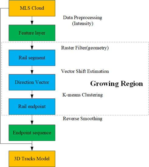
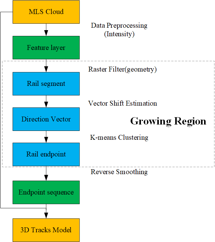
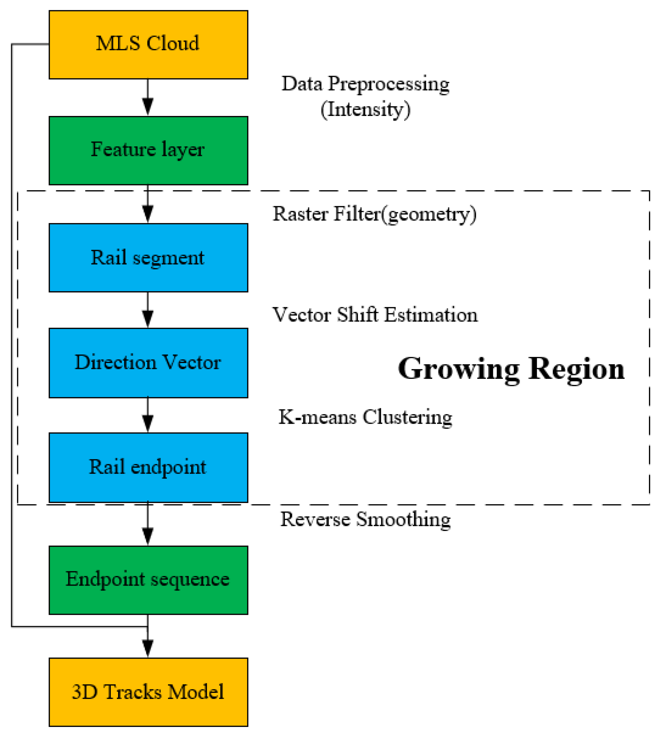
2. Methodology

Compared with other mainstream environmental sensing sensors (e.g., cameras), LiDAR has the advantages that can contain accurate three-dimensional spatial information, and it is not affected by illumination conditions. Railway tracks appear as thin elongated lines in MLS point clouds. Meanwhile, railway track tends to have specific reflectance properties in the wavelength ranges typically used in MLS systems, appearing as a homogeneous strip. The enormous amount of data from MLS system and the unique disordered spatial structure of MLS point clouds need to be handled in a specific way. According to the geometric and topological characteristics of the rail, the proposed region-growing estimation method fits the driving direction of the track model using vector shift estimation, and then it determines the precise location of the railway by clustering. Finally, the partial offset track points are corrected by reverse smoothing.

Figure 1 visually illustrates the workflow of the proposed approach to extract the railway track from the MLS data. The requisite input is only the MLS point clouds with intensity information, which does not depend on the trajectory data. First, point clouds with low intensity called “feature layer” are extracted from LIDAR data using the contrast between rail and other objects (e.g., sleeper and cushion), both of them are used to reduce the computational complexity and enable users to distinguish from the environment in terms of data density. For computational simplicity, the vector shift method was used to instead of least square to avoid the complex calculation caused by matrix inversion. The rail tracks can be divided into continuous segments by the direction-driven characteristics. In this paper, a region-growing format is used to connect each segment as the following two steps: (1) the vector shift is used to estimate the parameters (e.g., direction and center points), and (2) K-means clustering is used to calculate the starting point of the next segment. Subsequently, the estimated track endpoints deviation from the real track will be corrected based on point clouds in rail head extracted by the above method. Finally, the point clouds of rail tracks are extracted by the modified endpoints in the complete raw data. The following sections describe these steps in more detail.

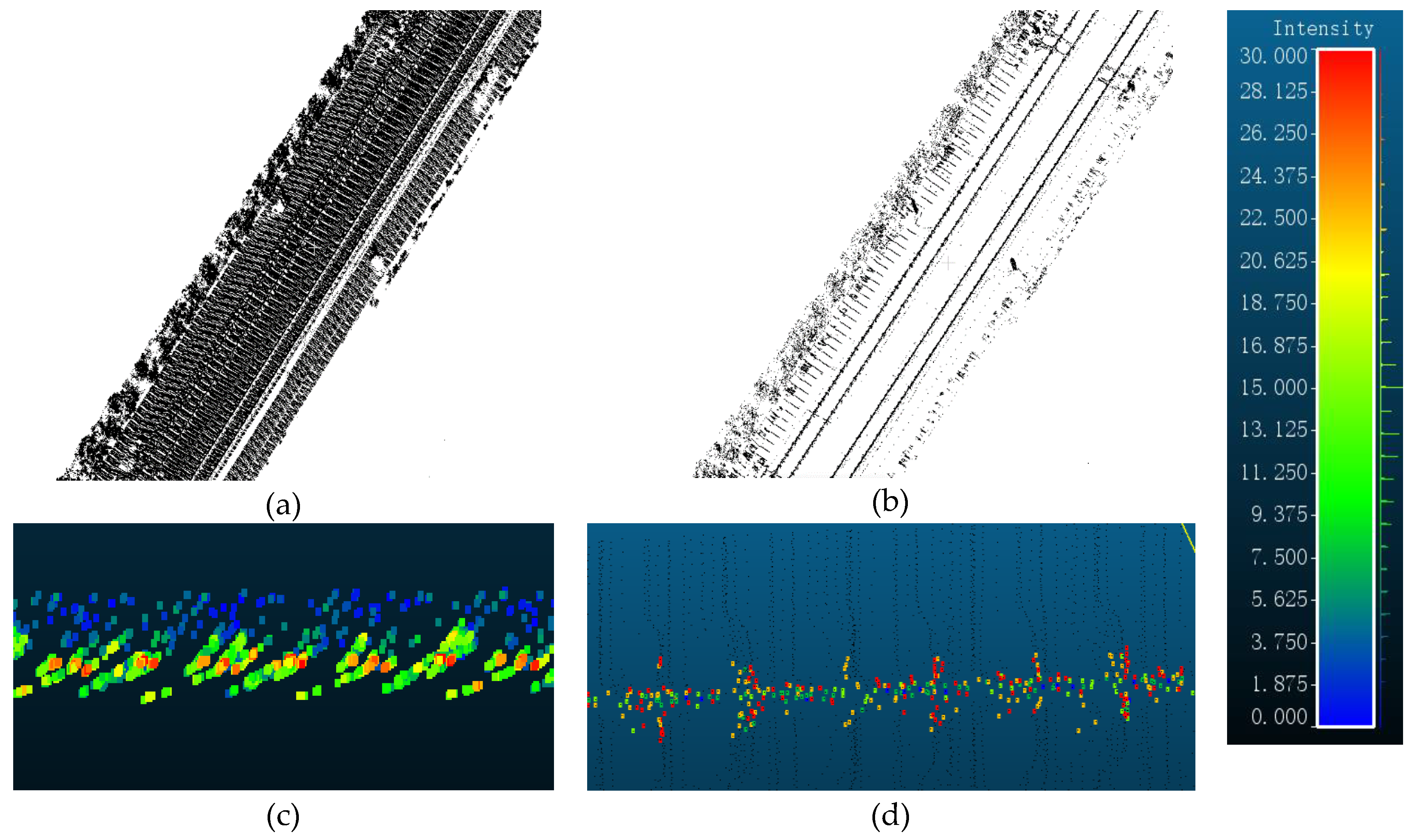
2.1. Data Preprocessing

The enormous amount of data from the MLS system affects the efficiency of data processing. To eliminate outliers, we reduced the computational complexity and improve the speed of the algorithm and adopted a data preprocessing method that keeps the structure of point clouds and greatly reduces the amount of data. The intensity data of the target recorded by LiDAR directly corresponds to the reflectance, so that the threshold method is used to extract the railway data point clouds. The MLS data detected in this paper is collected by Velodyne VLP-16 Lidar puck, whose intensity is classified into 256 levels. The reflective intensity of point clouds is mainly determined by the surface material of the reflective target. The rust on the track surface causes the reflective intensity to be lower than that of other objects in the environment. As shown in Figure 2b, setting the light intensity threshold of the railway to 3, this empirical method eliminated most of the interfering data (e.g., sleepers and padding) and the removed parts of points belong to the railway tracks. The lightweight data retaining the railway features is called “feature layers”. Compared with the raw data, the amount of data in the feature layer is greatly reduced. Using feature layer to determine the position of rail, rather than the raw data, helps reduce the computational complexity. As shown in Figure 2c,d, the intensity of the rails is low and the typical value is 0–3; however, the intensity of the sleepers is more than 20. Therefore, the intensity can be used as constrain to roughly separate the rails and sleepers, but the main purpose of using the intensity in the data preprocessing is to speed up the calculation. As the intensity does not fully identify the rails, the geometric constraints are added in the following steps.

2.2. Region Growing Estimation Method

2.2.1. Raster Filtering and Vector Shift Estimation

Feature layer eliminates the interference near rails, but the recorded data still contains other low-reflection objects. Due to the linear structure of the railway and the driving direction of the mobile mapping system, a pair of strips is used as a data processing unit space to detect the initial track regions and generate initial track models. The end connection of the polyline constitutes the broken track line. As shown in Formula (1), one section of rail is assumed as line model with endpoints $p_s$ and $p_e$ when any point $(x,y,z)$ of line through the point $p_s\left(x_s,y_s,z_s\right)$ and direction of vector $F\left(m,n,u\right)$, and their relationship is as follows.

$$\frac{x-x_s}{m}=\frac{y-y_s}{n}=\frac{z-z_s}{u}$$

(1)

Initialization track segment parameters $F^{\prime }\left(m_0,n_0,u_0\right)$ by bring the endpoint $p_e$ and creating a cylinder selection box which axis direction $F^{\prime }$. The radius of the cylinder is set at half of the standard gauge to ensure that there is only one rail except for the turnouts. As shown in the Figure 3a, the points in the cylindrical strip range are extracted for updating the driven-direction. According to the local geometric characteristics of rail, morphological filtering method is selected to extract rail head points. As shown in Figure 3b, these points are divided into horizontal grids. The grid is assumed containing rail, which difference of Z is greater than the threshold. The point has the largest Z value in one grid is extracted as rail head point (red points). As shown in Formula (2), these rail head points are used to calculate the updated driven-direction vector $F$. Compared with the least square method used in reference [44], it avoids matrix inversion and significantly reduces the computational complexity. The driven-direction $F^{\prime }$ is expressed as

$$F=\lambda {\displaystyle \sum }\left(p_i\left(x,y,z\right)-p_s\left(x_s,y_s,z_s\right)\right)$$

(2)

$$\lambda =\frac{1}{\sqrt{{({\displaystyle \sum }x-x_s)}^2+{({\displaystyle \sum }y-y_s)}^2+{({\displaystyle \sum }z-z_s)}^2}}$$

(3)

where $p_i$ is any rail head point which has been extracted in previous steps and $p_s$ is the prior designated start rail head point. As shown in Formula (3), $\lambda$ is calculated to make $F$ unitary. The rail head points are preserved as a sequence to form the basis of the reverse filter for correcting the track in Section 2.3.

2.2.2. K-means Clustering

Based on the above steps, the driven-direction vector $F\left(x,y,z\right)$ is obtained, and the approximate track points can be determined by multiplying the prior velocity scalar $l$. The extrapolation-based approach in [43] faced the same problem, and moreover they performed poorly in bends or switch rails. The pseudo-track points determined by the direction vector do not necessarily locate in the geometric center of the track. This is due to the inconsistency between the linear model of the track and the actually curved track itself. In this paper, a method for correcting rail points based on K-means clustering is proposed. First, the deviated pseudo-rail point is calculated, and then the data of rail area is extracted by K-means method, the endpoints are finally fitted by unbiased data points.

As shown in the Figure 4, data in the radius of search region is retrieved and used to calculate the centroid of rail track.

In Formula (4), the coordinate of pseudo-rail point $S$ will be calculated by driven-direction vector $F$ and the prior velocity scalar $l$.

$$\left[\begin{array}{c}{x}_s\\ y_s\\ z_s\end{array}\right]=\left[\begin{array}{c}{x}_{pi}\\ y_{pi}\\ z_{pi}\end{array}\right]+l\ast F$$

(4)

The raster processing algorithm mentioned in Section 2.2.1 is used to extract rail vertices in $S_R$ region. The next rail endpoint $P_{i+1}$ is the geometric center of each rail vertex. The calculated result of the endpoints sequence stores the spatial information of the rails. The K-means clustering method can avoid the interference of the switch rail at the turnout. The specific steps of this method are as follows.

The points are projected onto the normal plane of $F$. Comparing the angle of $F$ to X-axis and the angle of $F$ to Y-axis of the world coordinate system, the axis with smaller angle $\theta$ will be used for projection. Assuming that the angle between the normal vector $F$ and the X-axis of the geographic coordinate system is smaller, the point in range R will be projected.

Figure 5 demonstrates the K-means clustering algorithm. We randomly selected two points as the initial center of clusters, and then the distance between the point clouds to the initial center is calculated, and each point cloud is assigned to the subcluster whose center has nearest distance to it. The cluster center is recalculated each time when a point is assigned. Repeat this process until all the point clouds are assigned. The number of points within the radius $r$ of the standard rail section in the clusters center (blue dot in the circle in panels (a) and (b)) is taken as theirs density $D_l$ and $D_r$, separately. Then one cluster K-means is processed to obtain the center (yellow dot in the circle in panels (a) and (b)) and its density $D_c$. Compare the density $D_l$, $D_r$, and $D_c$, the cluster center with highest density is considered as the next rail endpoint.

The track consists of two parallel rails. We want to choose a better one to calculate the next track points. In fact, one rail of the track is often free from interference of switch rail, which enables to estimate the endpoints of the rail by calculation of the endpoints that are not interfered. The specific steps are as follows.

1. Comparing the angles between the direction vectors of the two rails and the direction vectors of the previous track segment, the direction vector of the rail with smaller angle is taken as the direction vector of the new track segment. As shown in Figure 6, the selected part of the red frame will be used to calculate the direction vectors of the track segment.

2. According to the K-means clustering method mentioned above, the endpoints of the non-interference track can be calculated.

3. The track endpoint with interference of switch rail is obtained by translating the non-interference rail endpoint to the vertical direction of the track direction by 1.435 m (standard gauge).

2.3. Reverse Smoothing

In the practical application of MLS system, when the point clouds are relatively sparse or interrupted, the fitting result of the track endpoints will deviate from the rail center. Using the previously extracted feature layer buffer data, the deviation between the track endpoints and the center of the actual track cross section is compensated by inverse filtering. As shown in Figure 7, reverse smoothing is based on the consideration of flat, only the plane position of the endpoint is modified. The specific steps are as follows.

• The point of track turnout cannot be smoothed in reverse. The error of the rail region of the endpoint $P_i$ can be calculated to exclude the point of turnout being relocated.
• The density of point $P_i$ compensated by reverse smoothing is less than two adjacent point $P_{i-1}$ and $P_{i+1}$.
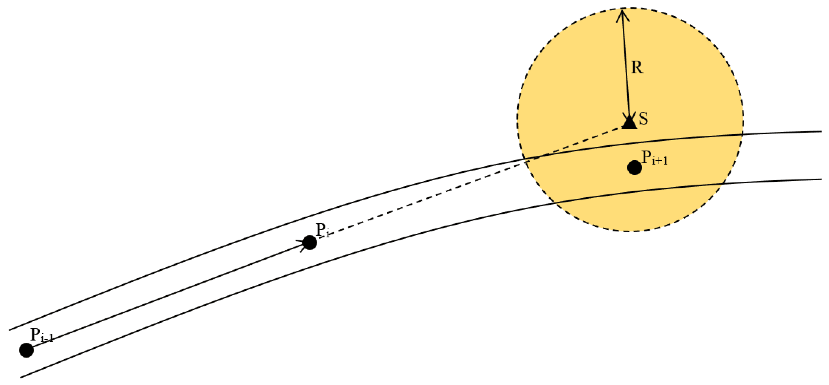
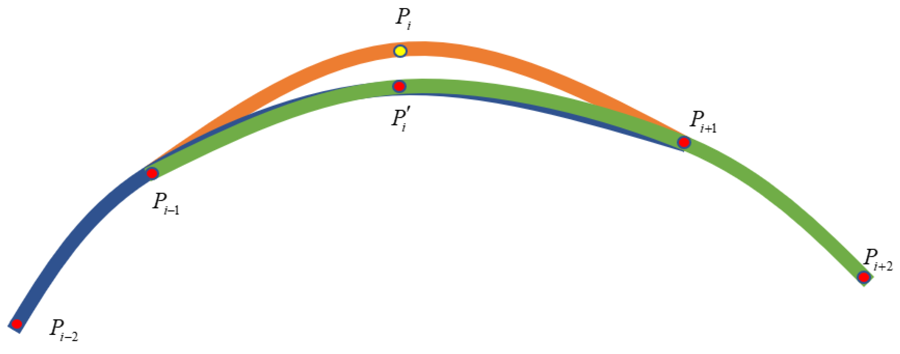
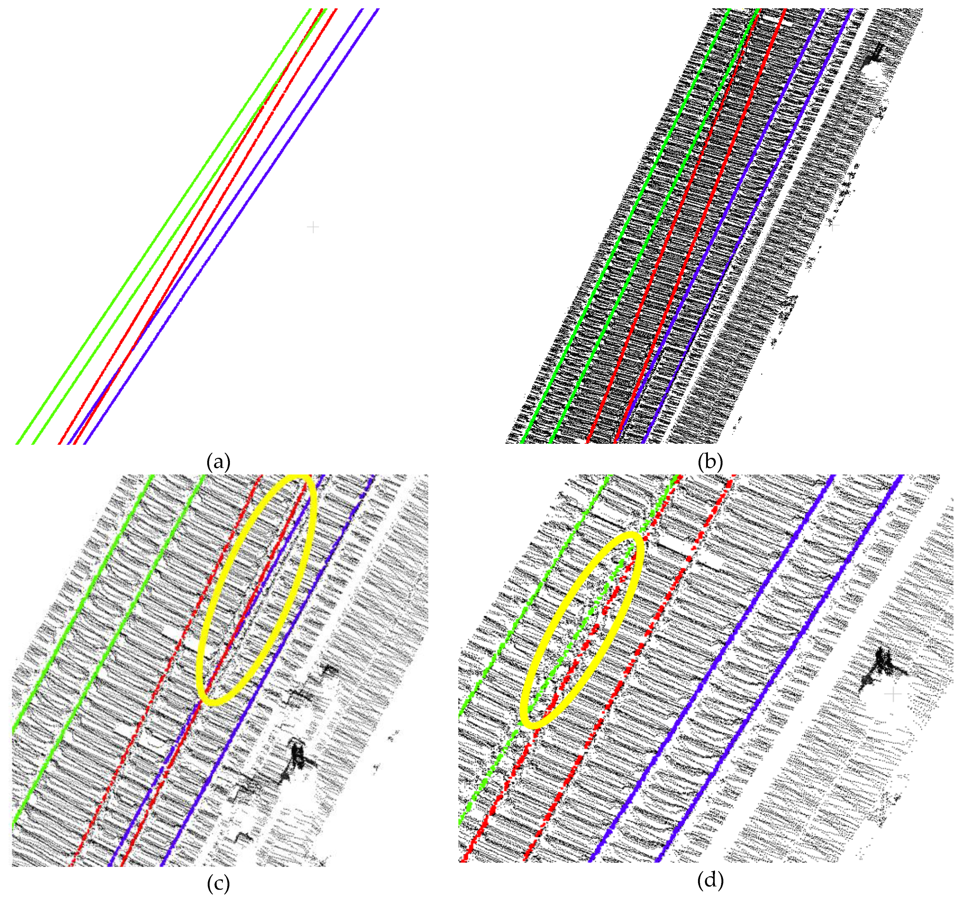
• As shown in the Figure 7, the two groups that are adjacent endpoints of $P_i\left(xi,yi,zi\right)$ are selected as blue and green lines, respectively, and a new endpoint $P_i{}^{\prime }\left(x{i}^{\prime },y{i}^{\prime },z{i}^{\prime }\right)$ is fitted by circular curve on plane expressed in the Formula (5). Bring the plane coordinates of $P_{i-2}$, $P_{i-1}$, and $P_{i+1}$ into the Formula (5) to get a set of parameters of the circular curve. The same process fits another circular curve by $P_{i-1}$, $P_{i+1}$ and, $P_{i+2}$ of the green line. Next, take $xi$ into these two functions. $y{i}^{\prime }$ is the average value of $y$ corresponding points in the two functions.

  $$A{x}^2+A{y}^2+Bx+Cy+D=0$$

  (5)
  If radius $RS$ of the functions is greater than empirical threshold 3000m, they’re considered lines. The following is the calculation formula (6) of radius $RS$.

  $$RS=\sqrt{\frac{B^2+C^2-4AD}{4A^2}}$$

  (6)
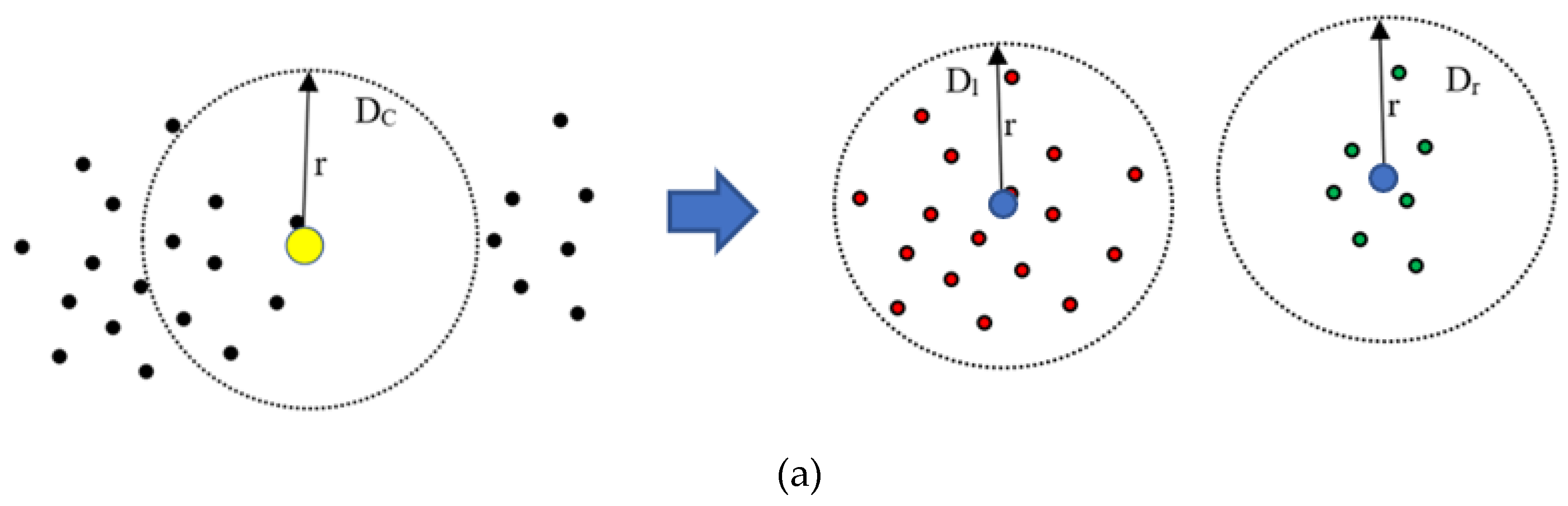
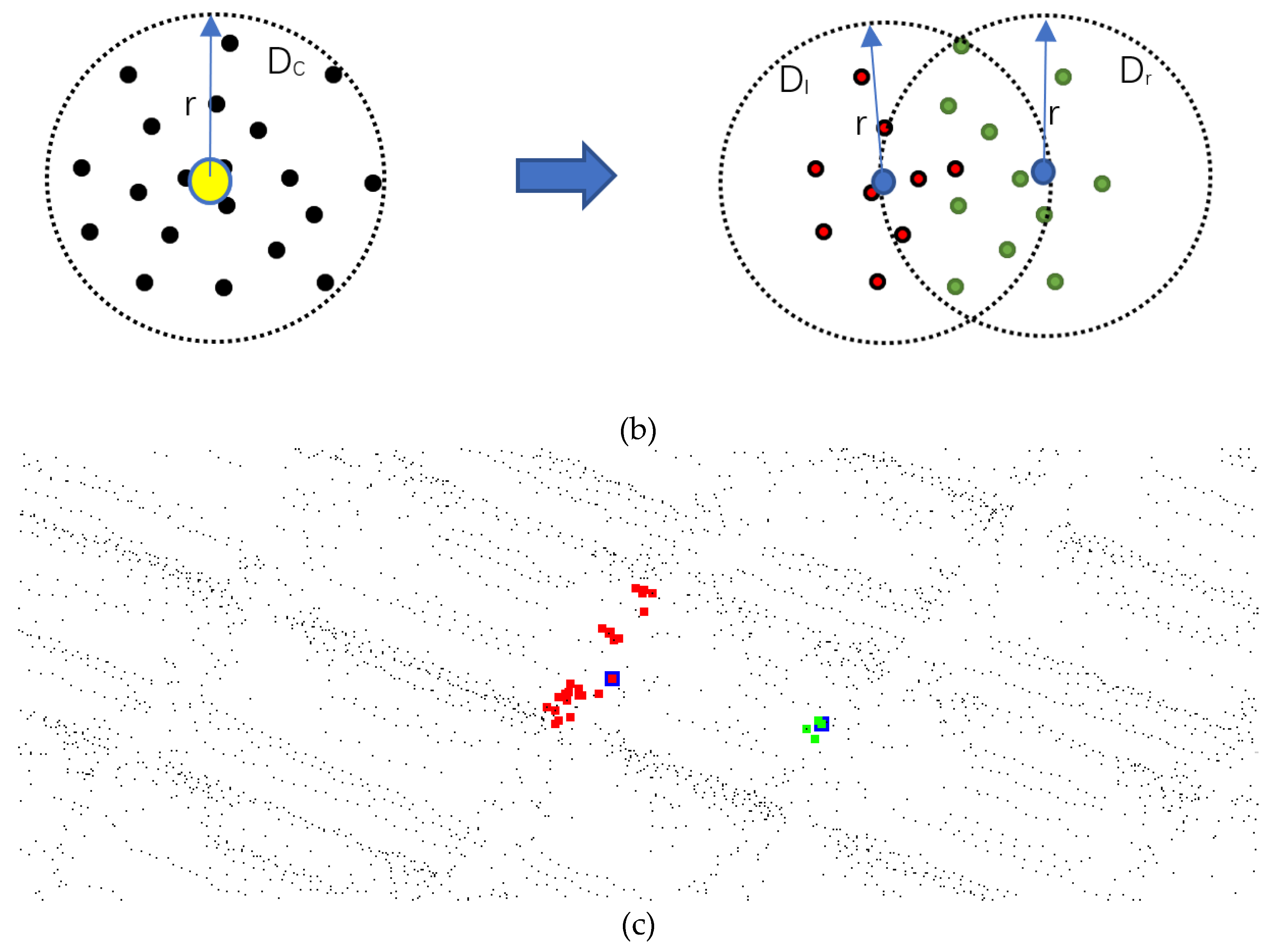
• Comparing the densities of clustering centers $P_i$ and $P_i^{\prime }$, which is the same as the density mentioned in Section 2.2.2. If the density of the corrected endpoint $P_i^{\prime }$ is significantly greater than that of the original endpoint $P_i$, the endpoint is corrected to $P_i{}^{\prime }$.

3. Environments and Data Description

3.1. Data Description

The experiments were undertaken with the test data captured by LiDAR Navigation and Environment Senescing Group of GNSS Research Center in Wuhan University. The Mapping System includes Lidar (Velodyne VLP-16 Lidar puck), an inertial navigation unit (MPSTNAV POS1100), a GNSS antenna (Novatel VEXXIS GNSS-800), and a storage computer. The data acquisition device is mounted on top of the railcar with an open top view, as shown in the Figure 8.

Using the navigation information from the navigation unit consisting of the GNSS antenna and the inertial navigation unit, the point clouds from the Lidar are transformed to the world coordinate systems.

LiDAR equipment is vertically placed to increase the number of echo points of rail tracks and catenary. The reflectivity of the object is calibrated and expressed by the intensity of light. There are different representations from 0 to 255. Diffuse reflectors report values from 0 to 100 for reflectivity from 0% to 100%. Retroreflectors report values from 101 to 255, where 255 represents an ideal reflection.

The navigation unit of this MLS system is an integrated GNSS/INS system. GNSS dual-frequency antenna can receive BDS+GPS satellite signals, and the inertial navigation unit POS1100 obtains position and pose information. The accuracy of point clouds used for classification is at centimeter level. The frequency of location data used to splice scanned data frames is higher than that of scanned data frames. We can obtain the final map with post-processing accuracy at centimeter level.

3.2. Test Area Description

The point clouds collected in the experiment cover the railway lines in Anhui province, China. Figure 9 illustrates an overview of the test area. We selected some representative experimental scenarios including linear, bends, turnouts, and track network. Using the no offset satellite remote sensing image from Map World as the base map, the superimposed point clouds visually indicate the accuracy of the point clouds. The train travels in the test area and the MLS system scans the environments around the rails at a fixed frequency of 10 Hz. The raw data of point clouds is resampled to eliminate point clouds density changes caused by the change of train speed. The average density of the point clouds is 490 points per square meter. The test area contains four typical scenarios in the process of train running. Straight line is the most basic condition of train running. Previous studies realized automatic track extraction under this scenario. In the case of bends and the tracks with height variation, as the tracks are designed to compensate the centrifugal force of train, the extraction is more difficult. In addition, the coexistence of multiple groups of rails makes data extraction in the scenario of a track network challenging.

4. Results and Discussion

To extract the rail point clouds, Jwa and Sonh used a method based on Kalman filter framework to preliminarily realize the rail extraction in the case of straight lines [43]. Inspired by the traditional regional growth method, this paper proposes an improved algorithm framework with high robustness and accuracy.

Table 1. Parameters used in the proposed method for rail extraction.

Parameter	Description	Values
LEN	Strip length (Straight-line) Strip length (Divided-deck) Strip length (bends)	15 m 15 m 8 m
R	Radius of pseudo-track point Raster size	0.3 m 0.15 m
INTEN	intensity threshold	5

shows strategies for extracting the rail point clouds, and the thresholds are discussed in Section 4.1.

4.1. Results

Lou et al. [20] used PCA to optimize the results of rail extraction. The raw point clouds were extracted by a method based on intensity and elevation difference. The remaining was used to estimate the largest eigenvector. But the PCA is sensitive to residuals (e.g., rail brace and switch rail), which made eigenvalue estimation difficult. Especially in the station environments shown in Figure 10c,d, these fixed clips are higher than the ground, which lead to more false negative points. In addition, PCA method failed due to the lack of a method to distinguish between stock rail and switch rail. In the regional growth method, the original point clouds are re-sampled from the endpoints of the rail to exclude outliers, and the rail points are identified based on spatial features.

Yang et al. [25] proposed a method based on template matching to extract the track. The track was divided into segments, which were localized by matching search on the cross section. The performance of this method depended on prior approximate location of the track and the flat ground. The complex topological structure of the track network and the inclination in bends would cause the wrong matching. In the reference [17], the track detection method based on section histogram and peak detection had fewer errors than the aforementioned template matching, but it still cannot solve the problem in tilted ground and track network. The method proposed in literature was based on peak detection and machine learning method SVM to further improve the accuracy of detection [18]. The region growing method proposed in this paper effectively solves the problem of track extraction in these two environments. As shown in Figure 11, after reverse smoothing and resampling, the fractured parts become connected and the sparse parts are supplemented.

Turnout is a kind of line connection equipment that enables trains to transfer from one track to another. It is also one of the weak links of track and it is usually laid in large quantities at stations or marshaling stations. Because the turnout is difficult for rail extraction, so in the past studies [43,44], it was always neglected. Around the railway station, the rails form a complex network of topological structures by interleaving turnouts. The Kalman method cannot distinguish two different tracks at the intersection of the tracks, and may even misestimate the direction, which will cause the early interruption of the estimation. According to the characteristics of two-dimensional LiDAR sensor, a template matching method was applied to extract the rail in the scene with track intersection [22]. However, this template matching method required higher accuracy of point clouds. As the distance between the sensor and the target increases, the reliability decreases rapidly. Only the nearest parallel tracks can be identified, which cannot meet the requirements of parallel extraction of multiple tracks near the station. In this paper, an improved clustering method is proposed, which can not only avoid the interference of intersection, but also effectively identify all tracks within the range of sensor accuracy. We selected both the turnouts and track network to further illustrate the situation of turnouts and crossing tracks. In the track-changing scenario in Figure 12, the track can be extracted without turnouts. With different colors, the segments of the turnouts can be clearly extracted and divided into different direction groups.

As shown in Figure 13, a more complex track network is formed, with seven tracks in different directions interlacing with each other. Different tracks are connected by turnouts. The improved regional growth method can also accurately identify the tracks in a complex railway network formed by interlacing seven different tracks. In order to show the extraction results, we intercept two sets of details as shown in panels (c) and (d).

4.2. Parameter Analysis

To check the robustness and sensitivity of endpoints estimation, the algorithm has been tested with different values for the strip length, width of strip, raster size. Section 4.3 provides quantitative evidence using two datasets acquired in the Bends and Turnouts of MLS test in VLP-16.

4.2.1. Strip Length

The MLS data of the tracks are discretized with a fixed section length along the driven-direction of the train. The time complexity of vector drift algorithm is proportional to the total data, the length of cross section has no effect on the calculation time, but reasonable length of track segment is the key to ensure robustness. The section length of 15m and 8m were empirically selected to be optimal for Divided-deck and bends respectively. In the divided-deck data group, there will be more ancillary facilities on both sides of the track, and false positive points will disturb the short section. However, compared with straight line and track separation, curve estimation is more susceptible to the increase of section length. When the length of the section is longer than 8 m, the curve track data violates the linear assumption of the strip length, which results in the interruption of the calculation process. Therefore, it is recommended that the section length is 8 m or 15 m.

4.2.2. Raster Size

Two different Raster filter methods have been experimented: one is to retain the point with maximum z, and the other is to retain the points at the top of the track. The scheme of retaining multiple points in the grid will not improve the accuracy of the track in linear, but will increase the ambiguity of the judgment of the intersection. As only one maximum point is reserved in a grid, the size of the grid has a great influence on the processing results. We hope to keep the linear characteristics of the rail as far as possible to eliminate false positive points, but the size of the grid should not be smaller than the size of the bottom. Too small a grid will lead to insufficient height difference in the grid and miss the rail head points. If the grid size is too large, the extracted data is sparse and a lot of information is lost. After several experiments, the best performance is obtained when the grid size is 30 cm.

4.3. Quantitative Evaluation

The results of the algorithm meet the visual requirements, and the accuracy will be quantitatively analyzed in this section. The manually extracted track is used as the standard for verification. The basic features of the standard rail are as follows: In the test area, the width of the bottom of the rail is 140 mm and the width of the top of the rail is 70 mm. A manually sized tag with a 35 mm wide buffer is considered as a real track. As shown in the

Table 2. The recognition of Sensitivity and Precision at point cloud level.

Method	Precision (%)	Sensitivity (%)
Kalman	82.28	91.96
Region growing	96.70	89.47

, the results are compared with those of the Kalman filter recursive framework. At the point clouds level, Equations (7) and (8) are used to calculate the Precision and Sensitivity.

$$Precision=\frac{tp}{tp+fp}$$

(7)

$$Sensitivity=\frac{tp}{tp+fn}$$

(8)

where $tp$ denotes the number of true positive points, which is the number of rail points found in both ground truth and detected data. $fp$ is the number of false positive points, which is the number of points that were detected but did not exist in ground truth. $fn$ denotes the number of false negative points, which is the number of rail points found in ground truth but were not found in detected data.

Table 2 lists the percentage of recognition Precision and Sensitivity in Kalman filtering and Region growing method. Kalman filter method extracts 48010 points, of which 39,501 points located in the true value region, with the Precision of 82.28%. Region growing method extracts 44,070 points, of which 42,615 points located in the true value region. The Precision of the improved Region growing method is 96.70%. As the outliers near the original rail are removed, the improved region growing method effectively improves the Precision of the extraction results. The outliers near the track are mainly the ancillary facilities such as fasteners of the track. Because the abnormal values near the original rail are removed, the improved region growth method can effectively improve the Precision of the extraction results even though the Sensitivity is slightly decrease. The outliers near the track are mainly accessory facilities such as track fasteners. In the scene of bends and track network, the track jams become more and more, so Kalman filtering method cannot accurately estimate the position of the next track. The methods for dealing with the straight lines are mature, and many related studies are reported. However, during the processing bends and turnouts, the method still needs further research. The turnout is the most difficult part in rail extraction, compared with previous study [22], which can detect straight lines well, the proposed method in this paper greatly extend the application scenarios including challenging railway sections, such as bends and turnouts. We analyze the results using the improved region growing method. As shown in

Table 3. The Precision and Sensitivity in complex environments.

Scene	Precision (%)	Sensitivity (%)
Bends	90.32	83.27
Turnouts	81.31	83.33

, it is the Precision and Sensitivity of the improved region growing method in specific scenarios, the Precision in Bends can reach 90.32%, and for turnout, the Precision is more than 80%.

5. Conclusions

The accurate management of rail transit system depends on the accurate space information of rail track, which is of great significance to the safety of train operation. Based on improved region growing method, this paper presents a novel framework of automatic track extraction for MLS data independent of location trajectory. A self-built MLS system was used for data collection and a total of 80 million points were selected as test data. The average density of dots is approximately 490 points per square meter. The proposed method can extract all the rails in the sensor coverage area simultaneously, and can adapt to the conditions of railway network with large radian (e.g., bends and turnout). First, light intensity data is used to separate the rail tracks from the concrete sleeper preliminarily. Then, a vector shift algorithm is used to calculate the trajectory driving direction. Next, the cluster-based algorithm is used to check label of track by separating the target and switch track. Finally, the proposed method was tested outdoors with a real-world railcar on different configurations: linear rails, bends, and turnouts in railway network. The experiments show that the proposed method can correctly identifies rail tracks and performs well in complex situations with multiple disturbances.

This study validates the feasibility of extracting railway parts even at bends and turnouts from MLS data. Based on the traditional views, railway tracks are spatial features with accurate spatial location. It is expected that the extracted features will be used to improve the positioning accuracy in future research. Although the present implementation of the algorithm in C++ is not yet running in real-time, it is believed that it will be implemented in real time during the improved implementation, which provides great potential for using the algorithm in real-time in railway environment sensing. Therefore, it is an important progress for the autonomous driving system in railway domain.

References

- Yu, X.; Lang, M.; Gao, Y.; Wang, K.; Su, C.-H.; Tsai, S.-B.; Huo, M.; Yu, X.; Li, S. An Empirical Study on the Design of China High-Speed Rail Express Train Operation Plan-From a Sustainable Transport Perspective. Sustainability 2018, 10, 2478. [Google Scholar] [CrossRef]
- Ma, L.; Li, Y.; Li, J.; Wang, C.; Wang, R.; Chapman, M. Mobile Laser Scanned Point-Clouds for Road Object Detection and Extraction: A Review. Remote Sens. 2018, 10, 1531. [Google Scholar] [CrossRef]
- Liu, J.; Liang, H.; Wang, Z.; Chen, X. A Framework for Applying Point Clouds Grabbed by Multi-Beam LIDAR in Perceiving the Driving Environment. Sensors 2015, 15, 21931–21956. [Google Scholar] [CrossRef] [PubMed]
- Al-Bayari, O. Mobile mapping systems in civil engineering projects (case studies). Appl. Geomat. 2019, 11, 1–13. [Google Scholar] [CrossRef]
- Dabeer, O.; Ding, W.; Gowaiker, R.; Grzechnik, S.K.; Lakshman, M.J.; Lee, S.; Reitmayr, G.; Sharma, A.; Somasundaram, K.; Sukhavasi, R.T.; et al. An end-to-end system for crowdsourced 3D maps for autonomous vehicles: The mapping component. In Proceedings of the 2017 IEEE/RSJ International Conference on Intelligent Robots and Systems (IROS), Vancouver, BC, Canada, 24–28 September 2017; pp. 634–641. [Google Scholar]
- Paterson, S.; Sheriff, C.; Ferguson, J. Metrolinx’s Toronto Electrification Project: Phase 1-the Engineering Survey. In Proceedings of the ASME Joint Rail Conference, 2017; AMER Soc Mechanical Engineers: Three Park Avenue, New York, NY, USA, 4–7 April 2017. [Google Scholar]
- Salah, I.B.; Kramm, S.; Demonceaux, C.; Vasseur, P. Summarizing Large Scale 3D Mesh. In Proceedings of the 2018 IEEE/RSJ International Conference on IN℡Ligent Robots and Systems (IROS), New York, NY, USA, 1–5 October 2018; pp. 6372–6377. [Google Scholar]
- Li, W.; Meng, X.; Wang, Z.; Fang, W.; Zou, J.; Li, H.; Sun, T.; Liang, J. Low-cost vector map assisted navigation strategy for autonomous vehicle. In Proceedings of the 2018 IEEE Asia Pacific Conference on Circuits and Systems (APCCAS 2018), New York, NY, USA, 26–30 October 2018; pp. 536–539. [Google Scholar]
- Hao, C.-Y.; Chen, M.-H.; Chou, T.-Y.; Lin, C.-W. Design of a Resource-oriented Framework for Point Cloud Semantic Annotation with Deep Learning. In Proceedings of the 2018 IEEE FIRST International Conference on Artificial IN℡Ligence and Knowledge Engineering (AIKE), New York, NY, USA, 26–28 September 2018; pp. 228–233. [Google Scholar]
- Che, E.; Jung, J.; Olsen, M. Object Recognition, Segmentation, and Classification of Mobile Laser Scanning Point Clouds: A State of the Art Review. Sensors 2019, 19, 810. [Google Scholar] [CrossRef]
- Tomljenovic, I.; Hoefle, B.; Tiede, D.; Blaschke, T. Building Extraction from Airborne Laser Scanning Data: An Analysis of the State of the Art. Remote Sens. 2015, 7, 3826–3862. [Google Scholar] [CrossRef]
- Matikainen, L.; Lehtomaki, M.; Ahokas, E.; Hyyppa, J.; Karjalainen, M.; Jaakkola, A.; Kukko, A.; Heinonen, T. Remote sensing methods for power line corridor surveys. ISPRS J. Photogramm. Remote Sens. 2016, 119, 10–31. [Google Scholar] [CrossRef]
- Li, F.; Lehtomäki, M.; Oude Elberink, S.; Vosselman, G.; Kukko, A.; Puttonen, E.; Chen, Y.; Hyyppä, J. Semantic segmentation of road furniture in mobile laser scanning data. ISPRS J. Photogramm. Remote Sens. 2019, 154, 98–113. [Google Scholar] [CrossRef]
- Wang, Z.; Wu, X.; Yan, Y.; Jia, C.; Cai, B.; Huang, Z.; Wang, G.; Zhang, T. An Inverse Projective Mapping-based Approach for Robust Rail Track Extraction. In Proceedings of the 2015 8th International Congress on Image and Signal Processing (CISP), New York, NY, USA, 14–16 October 2015; pp. 888–893. [Google Scholar]
- Liu, Z.; Liu, W.; Han, Z. A High-Precision Detection Approach for Catenary Geometry Parameters of Electrical Railway. IEEE Trans. Instrum. Meas. 2017, 66, 1798–1808. [Google Scholar] [CrossRef]
- Pastucha, E. Catenary System Detection, Localization and Classification Using Mobile Scanning Data. Remote Sens. 2016, 8, 801. [Google Scholar] [CrossRef]
- Arastounia, M. Automated Recognition of Railroad Infrastructure in Rural Areas from LIDAR Data. Remote Sens. 2015, 7, 14916–14938. [Google Scholar] [CrossRef]
- Sánchez-Rodríguez, A.; Riveiro, B.; Soilán, M.; González-deSantos, L.M. Automated detection and decomposition of railway tunnels from Mobile Laser Scanning Datasets. Autom. Constr. 2018, 96, 171–179. [Google Scholar] [CrossRef]
- Chen, C.; Yang, B.; Song, S.; Peng, X.; Huang, R. Automatic Clearance Anomaly Detection for Transmission Line Corridors Utilizing UAV-Borne LIDAR Data. Remote Sens. 2018, 10, 613. [Google Scholar] [CrossRef]
- Lou, Y.; Zhang, T.; Tang, J.; Song, W.; Zhang, Y.; Chen, L. A Fast Algorithm for Rail Extraction Using Mobile Laser Scanning Data. Remote Sens. 2018, 10, 1998. [Google Scholar] [CrossRef]
- Qiu, K.; Sun, K.; Ding, K.; Shu, Z. A Fast and Robust Algorithm for Road Edges Extraction from Lidar Data. ISPRS Int. Arch. Photogramm. Remote Sens. Spat. Inf. Sci. 2016, XLI-B5, 693–698. [Google Scholar] [CrossRef]
- Stein, D.; Spindler, M.; Lauer, M. Model-based rail detection in mobile laser scanning data. In Proceedings of the 2016 IEEE Intelligent Vehicles Symposium (IV), Gotenburg, Sweden, 19–22 June 2016; pp. 654–661. [Google Scholar]
- Arastounia, M.; Oude Elberink, S. Application of Template Matching for Improving Classification of Urban Railroad Point Clouds. Sensors 2016, 16, 2112. [Google Scholar] [CrossRef]
- Oude Elberink, S.; Khoshelham, K.; Arastounia, M.; Diaz Benito, D. Rail Track Detection and Modelling in Mobile Laser Scanner Data. ISPRS Ann. Photogramm. Remote Sens. Spat. Inf. Sci. 2013, II-5/W2, 223–228. [Google Scholar] [CrossRef]
- Yang, B.; Fang, L. Automated Extraction of 3-D Railway Tracks from Mobile Laser Scanning Point Clouds. IEEE J. Sel. Top. Appl. Earth Obs. Remote Sens. 2014, 7, 4750–4761. [Google Scholar] [CrossRef]
- Leary, R.D.; Brennan, S.N. Extracting Geometric Road Centerline and Lane Edges from Single-Scan LiDAR Intensity Using Optimally Filtered Extrema Features. In Proceedings of the 2018 IEEE Conference on Control Technology and Applications (CCTA), Copenhagen, Denmark, 21–24 August 2018; pp. 1133–1138. [Google Scholar]
- Andani, M.T.; Mohammed, A.; Jain, A.; Ahmadian, M. Application of LIDAR technology for rail surface monitoring and quality indexing. Proc. Inst. Mech. Eng. Part F J. Rail Rapid Transit 2018, 232, 1398–1406. [Google Scholar] [CrossRef]
- Gorte, B.; Oude Elberink, S.; Sirmacek, B.; Wang, J. IQPC 2015 Track: Tree Separation and Classification in Mobile Mapping Lidar Data. ISPRS Int. Arch. Photogramm. Remote Sens. Spat. Inf. Sci. 2015, XL-3/W3, 607–612. [Google Scholar] [CrossRef]
- Telke, C.; Quarz, V.; Beitelschmidt, M.; Schulz, A. A novel modular measurement system for the development of light rail vehicles. In The Dynamics of Vehicles on Roads and Tracks; Osenberger, M., Plochl, M., Six, K., Edelmann, J., Eds.; CRC Press: Boca Raton, FL, USA, 2016; pp. 1451–1460. [Google Scholar]
- Tang, C.; Tian, G.Y.; Chen, X.; Wu, J.; Li, K.; Meng, H. Infrared and visible images registration with adaptable local-global feature integration for rail inspection. Infrared Phys. Technol. 2017, 87, 31–39. [Google Scholar] [CrossRef]
- Li, S.; Xu, C.; Chen, L.; Liu, Z. Speed Regulation of Overhead Catenary System Inspection Robot for High-Speed Railway through Reinforcement Learning. In Proceedings of the 2018 IEEE Smartworld, Ubiquitous IN℡Ligence & Computing, Advanced & Trusted Computing, Scalable Computing & Communications, Cloud & Big Data Computing, Internet of People and Smart City Innovation (SMARTWORLD/SCALCOM/UIC/ATC/CBDCOM/IOP/SCI), New York, NY, USA, 8–12 October 2018; pp. 1378–1383. [Google Scholar]
- Wang, A.; He, X.; Ghamisi, P.; Chen, Y. LiDAR Data Classification Using Morphological Profiles and Convolutional Neural Networks. IEEE Geosci. Remote Sens. Lett. 2018, 15, 774–778. [Google Scholar] [CrossRef]
- Rachmadi, R.F.; Uchimura, K.; Koutaki, G.; Ogata, K. Road edge detection on 3D point cloud data using Encoder-Decoder Convolutional Network. In Proceedings of the 2017 International Electronics Symposium on Knowledge Creation and Intelligent Computing (IES-KCIC), Surabaya, Indonesia, 26–27 September 2017; pp. 95–100. [Google Scholar]
- Su, H.; Maji, S.; Kalogerakis, E.; Learned-Miller, E. Multi-view Convolutional Neural Networks for 3D Shape Recognition. In Proceedings of the 2015 IEEE International Conference on Computer Vision (ICCV), New York, NY, USA, 7–13 December 2015; pp. 945–953. [Google Scholar]
- Qin, N.; Hu, X.; Dai, H. Deep fusion of multi-view and multimodal representation of ALS point cloud for 3D terrain scene recognition. ISPRS J. Photogramm. Remote Sens. 2018, 143, 205–212. [Google Scholar] [CrossRef]
- Maturana, D.; Scherer, S. VoxNet: A 3D Convolutional Neural Network for Real-Time Object Recognition. In Proceedings of the 2015 IEEE/RSJ International Conference on IN℡Ligent Robots and Systems (IROS), New York, NY, USA, 28 September–2 October 2015; pp. 922–928. [Google Scholar]
- Huang, J.; You, S. Point Cloud Labeling using 3D Convolutional Neural Network. In Proceedings of the 2016 23rd International Conference on Pattern Recognition (ICPR), Cancun, Mexico, 4–8 December 2016; pp. 2670–2675. [Google Scholar]
- Qi, C.R.; Su, H.; Mo, K.; Guibas, L.J. PointNet: Deep Learning on Point Sets for 3D Classification and Segmentation. In Proceedings of the 30th IEEE Conference on Computer Vision and Pattern Recognition (CVPR 2017), Honolulu, HI, USA, 21–26 July 2017; pp. 77–85. [Google Scholar]
- Hackel, T.; Wegner, J.D.; Savinov, N.; Ladicky, L.; Schindler, K.; Pollefeys, M. Large-Scale Supervised Learning For 3D Point Cloud Labeling: Semantic3d.Net. Photogramm. Eng. Remote Sens. 2018, 84, 297–308. [Google Scholar] [CrossRef]
- Zhou, W.; Peng, R.; Dong, J.; Wang, T. Automated extraction of 3D vector topographic feature line from terrain point cloud. Geocarto Int. 2018, 33, 1036–1047. [Google Scholar] [CrossRef]
- Qin, X.; Wu, G.; Lei, J.; Fan, F.; Ye, X. Detecting Inspection Objects of Power Line from Cable Inspection Robot LiDAR Data. Sensors 2018, 18, 1284. [Google Scholar] [CrossRef]
- Zhang, S.; Wang, C.; Yang, Z.; Chen, Y.; Li, J. Automatic Railway Power Line Extraction Using Mobile Laser Scanning Data. Int. Arch. Photogramm. Remote Sens. Spat. Inf. Sci. 2016, XLI-B5, 615–619. [Google Scholar] [CrossRef]
- Jwa, Y.; Sonh, G. Kalman Filter Based Railway Tracking from Mobile Lidar Data. ISPRS Ann. Photogramm. Remote Sens. Spat. Inf. Sci. 2015, II-3/W5, 159–164. [Google Scholar] [CrossRef]
- Mohamad, M.; Kusevic, K.; Mrstik, P.; Greenspan, M. Automatic Rail Extraction in Terrestrial and Airborne LiDAR Data. In Proceedings of the 2013 International Conference on 3D Vision-3DV 2013, Seattle, WA, USA, 29 June–1 July 2013; pp. 303–309. [Google Scholar]