Article

A Composite Method for Predicting Local Accuracies in Remotely Sensed Land-Cover Change Using Largely Non-Collocated Sample Data

1
School of Sociology, Wuhan University, Wuhan 430072, China
2
School of Geodesy and Geomatics, Wuhan University, Wuhan 430079, China
3
State Key Laboratory for Information Engineering in Surveying, Mapping and Remote Sensing, Wuhan University, Wuhan 430079, China
4
School of Geology Engineering and Geomatics, Chang’an University, Xi’an 710054, China
5
Beijing Institute of Surveying and Mapping, Beijing 100038, China
*
Author to whom correspondence should be addressed.
Remote Sens. 2019, 11(23), 2818; https://doi.org/10.3390/rs11232818
Submission received: 28 October 2019 / Revised: 25 November 2019 / Accepted: 26 November 2019 / Published: 28 November 2019

Abstract

:
As in conventional error matrix-based accuracy assessments, collocated reference sample data are often used for characterizing per-pixel (local) accuracies in land-cover change maps so that local accuracy predictions can be made using direct methods. In that way, correctness in “from-to” change categorization at sample pixels is assessed and modeled directly. To circumvent the issue of reference sample data being non-collocated, as is often the case for sample data collected independently for mono-temporal reference land-cover labeling or those added necessarily to reflect landscape changes, the PXCOV (Product rule with adjustment for cross-COVariance between single-date classification correctness) method was developed previously. However, the use of PXCOV becomes complicated when few or no collocated sample data are available and cross-validation cokriging, a procedure involving non-trivial geostatistical modeling, has to be incurred for estimation of cross-correlation. To overcome PXCOV’s lack of practicality when using mostly non-collocated sample data, this paper presents a simple alternative. It is furnished through stratified approximation of cross-correlation and features combined use of minimum and multiplication operators. Specifically, in this composite method (named Fuzzy+Product), minimum operator (resembling fuzzy set “min” operator and thus named Fuzzy) is applied over no-change pixels stratum where maximum correlation is assumed, while multiplication operator (i.e., product rule named Product) is applied for change pixels stratum where cross-correlation is assumed negligible (i.e., minimum correlation), without having to run cross-validation cokriging as in PXCOV. Studies were undertaken to test the proposed method based on datasets collected previously concerning GlobeLand30 2000 and 2010 land-cover at five sites in China. For each site, five model-training samples (being mostly non-collocated) of equal sizes and one independent model-testing sample (collocated) were used. Logistic regression models fitted with relevant sample data were applied to predict local accuracies in single-date classifications using selected map class occurrence pattern indices quantified in optimized moving windows. The area under the curve (AUC) of the receiver operating characteristic was used for evaluating alternative methods. Empirical results confirmed that method Fuzzy+Product is more accurate than both Fuzzy and Product in general and there are no statistically significant differences between it and PXCOV. This indicates Fuzzy+Product being a method of relative simplicity but reasonable accuracy when reference data are non-collocated or mostly so. Its value is likely best manifested when local and global accuracy characterization in multi-temporal change information (discrete and fractional) is concerned.

Graphical Abstract

1. Introduction

Land-cover information is important for landscape characterization and environmental monitoring [1,2]. A variety of land-cover information products is generated from different remote-sensing systems [3,4,5]. They depict both static cover types and dynamic changes in space and time. For example, after release of four National Land Cover Database (NLCD) products over the past two decades: NLCD 1992, 2001, 2006, and 2011, the U.S. Geological Survey (USGS) has designed a new generation of NLCD products named NLCD 2016 to further establish a long-term monitoring capability for land resources [6]. Time series of land-cover maps are also common [7,8]. While land-cover information is conventionally represented in categorical format (i.e., encoded as discrete cover types and/or change class labels), fractional representations of land-cover and change also become popular [9,10,11], although this paper focuses on the former type of land-cover change maps.
Scientific replicability and practical usefulness of land-cover information products depend on their accuracy. However, no land-cover or change maps created from computer processing of remotely sensed images and auxiliary data can be completely accurate [12,13]. Even visual interpretation of remote-sensing images cannot guarantee absolute accuracy in resultant maps. It is thus important to build up accuracy assessment capabilities in production and use of land-cover information. There is increasing research and developments on accuracy assessments in the aforementioned different types of land-cover information products [14,15,16,17].
The conventional way to describe accuracies in land-cover and land-cover change maps is through error matrices, from which we can obtain some global summary of map accuracies in terms of overall, user’s, and producer’s accuracies [14,17,18]. However, we may not be able to get any information about spatial variation of accuracies below individual map classes from these non-spatial (or global) accuracy metrics. In contrast, local accuracy descriptors would better support exploratory and diagnostic analyses of spatial distributions of misclassification errors, hence, better guiding classifier improvements and information fusion. Spatialized accuracy characterization in land-cover information products has thus drawn increasing research attention, for both static land-cover classification and dynamic change-categorization [19,20,21,22,23,24,25,26,27,28]. Useful reviews are given in Khatami et al. [29], Zhang et al. [30], and Zhang et al. [31].
For quantification of local accuracies in change maps specifically, reference sample data are essential as in conventional non-spatial accuracy assessments. It is preferable to have collocated sample data to verify true cover types at the same locations but different times to get the information about correctness of change categorization for individual locations (i.e., map pixels) [32,33,34]. However, collocated sample data may be far from enough or even unavailable. On the other hand, non-collocated sample data are common for reference data collected for mono-temporal maps without consideration or coordination for change analysis [35]. Such non-collocated data’s assembling and re-use would help save cost of sampling, especially for ground-based surveys. Re-use of non-collocated sample data may be made directly or, more effectively, in combination with additionally acquired sample data. The latter option can be furnished by augmented sample design [36], which is built from a base design say stratified random sampling (StRS) as used in Zhang et al. [31]. We may collect new sample data at locations where changes are observed, while collecting repeating sample data at some of prior sampled locations, with the aim to allocate sample units to strata of “from-to” classes according to recommendations [37].
Accordingly, there are two broad types of methods for mapping local accuracies in land-cover change maps: direct and indirect, as in change analysis [38]. In the former, collocated sample data are assumed so that methods designed for mono-temporal land-cover maps can be directly extended to bi-temporal change maps [27,39]. The latter caters for non-collocated sample data and is based on mono-temporal accuracy analyses and their proper synthesis [31]. It plays an increasingly important role in change analyses and accuracy assessments since sample designs become necessarily complexly configured due to the need to monitor the changing landscape [40]. Zhang et al. [31] proposed an indirect method, which is actually Method Product with adjustment for cross-correlation (i.e., temporal correlation) in bi-temporal classification correctness (hence named PXCOV to stand for Product with adjustment for cross(X)-COVariance). Method Product evaluates probabilities of correct change-classification as multiplication of probabilities of correct mono-temporal classifications; the multiplication operator was previously used by Steele [41] and Pontius and Cheuk [42] for constructing combined classifiers and comparing fuzzy maps, respectively. Using PXCOV, it is possible to utilize all reference sample data available, regardless of their being collocated or not, contributing to cost-saving in sampling for reference data. This is facilitated by estimating local accuracies in single-date classifications and then synthesizing them properly through accommodating temporal correlation between single-date accuracies. However, its practicality is limited by the need to estimate temporal correlation via cross-validation cokriging (a relatively complicated procedure of geostatistical modeling and computing) when collocated sample data are not available or insufficient (i.e., when sample data available are non-collocated or mostly so).
To overcome PXCOV’s lack of practicality, this paper presents a simple alternative method. It is furnished through stratified approximation of temporal correlation in change-classification accuracies and features combined use of minimum and multiplication operators. Specifically, in this composite method (named Fuzzy+Product), minimum operator (resembling fuzzy set “min” operator, thus named Fuzzy) is applied over non-change pixels whereas maximum correlation is assumed so that minimum values of predicted probabilities of correct classifications in single-date maps are taken as approximation for probabilities of correct change-classification at individual no-change pixels [42,43]. For change pixels where temporal correlation is usually very weak and thus assumed zero approximately, multiplication operator (i.e., the product rule [31,42] named Product) is applied. Thus, using Fuzzy+Product, we can estimate local accuracies in change-classification easily through combined use of minimum operator (over no-change pixels) and multiplication operator (over change pixels), without having to run the complicated procedure of cross-validation cokriging iteratively as in the original PXCOV implementation.
The research question concerns whether Fuzzy+Product is a reasonably accurate method in comparison with PXCOV while being simpler than PXCOV. Thus, the objective of this paper is to investigate performances of the proposed method Fuzzy+Product relative to alternative methods including PXCOV. As is demonstrated by the experimental results, the answer is positive.
Fuzzy+Product’s benefits are summarized below. First, it is simpler than PXCOV without compromising accuracy. Second, it holds great potentials for future applications in accuracy characterization in the context of multi-temporal change analyses, while PXCOV is oriented to bi-temporal settings only, as is discussed in Section 4.2. Third, its extension to accuracy analyses in fractional (change) classifications is also promising (see Section 4.2). Lastly, it facilitates local-global-combined accuracy assessments and modeling with uncertainty quantified while benefitting area estimate corrections, as discussed in Section 4.3. These advantages manifest themselves well in the scenarios where reference sample data are non-collocated, or mostly so.
Some clarification about this research in comparison with the work underlying PXCOV [31] is in place here. First, Fuzzy+Product works by stratified approximation of cross-correlation between single-date classification accuracies rather than relying on complicated geostatistical modeling as in PXCOV when there are no or few collocated sample data. Although we used the same datasets as in [31], the major thrust of contribution in this research is not repetition of the work in [31]. Second, we focus explicitly on applications of Fuzzy+Product (in comparisons with alternative indirect methods) using largely non-collocated data while applications of PXCOV were discussed (mainly in comparisons with direct methods) using both non-collocated and collocated data.
The remainder of the article is as follows. In Section 2, we first describe the study sites and datasets. Five training sample sets of equal sizes with different but dominating proportions of non-collocated sample pixels, which were collected at five study sites in China in previous research [31], were used. This is followed by a description of the proposed method Fuzzy+Product along with alternative methods: PXCOV, Fuzzy, and Product, with the latter two methods applied to all pixels regardless of them being change or no-change pixels. Section 3 describes the results of empirical studies aiming to test and compare the performances of these methods on the basis of independent validation sample data. Finally, Section 5 concludes the paper after some discussion in Section 4.

2. Materials and Methods

2.1. Study Area and Datasets

This research is based on the same five sites in China (each of 9 km by 9 km in areal extent) as in Zhang et al. [31], as shown in Figure 1. They are labeled CE (center), NE (northeast), NW (northwest), SW (southwest), and SE (southeast), to reflect their relative geographic locations. Site CE is located in Xi’an, Shaanxi Province, which lies in the center of China. Site NE is situated in Harbin, Heilongjiang Province, northeast of China. Site NW lies in Fukang, Xinjiang Uygur Autonomous Region, northwest of China. Site SW is in Kunming, Yunnan, southwest of China, and SE is located in Ganzhou, Jiangxi Province, southeast of China. As in Zhang et al. [31], GlobeLand30 land cover datasets (for year 2000 and 2010) of the study area were employed in this research. GlobeLand30 is a global fine-resolution (30 m spatial resolution) land-cover information product produced by the National Geomatics Center of China [5]. As an open-access global land cover product, GlobelLand30 was extracted from >20,000 Landsat and Chinese HJ-1 satellite images using a pixel-objected-knowledge (POK)-based operational mapping approach, with an estimated overall classification accuracy of over 80%, on average, for single-date land cover [5]. For China, there are 10 land-cover types [5], although only six cover types (i.e., water bodies, artificial surfaces, cultivated land, forest, grassland, and bare land) are present in these sites as a whole. The definition of the six land cover types according to GlobelLand30 classification system is shown in Table 1. Except for site NW, the dominant class of the other four sites is cultivated land and artificial surfaces, which reflect the profound impact of human activities on land cover.
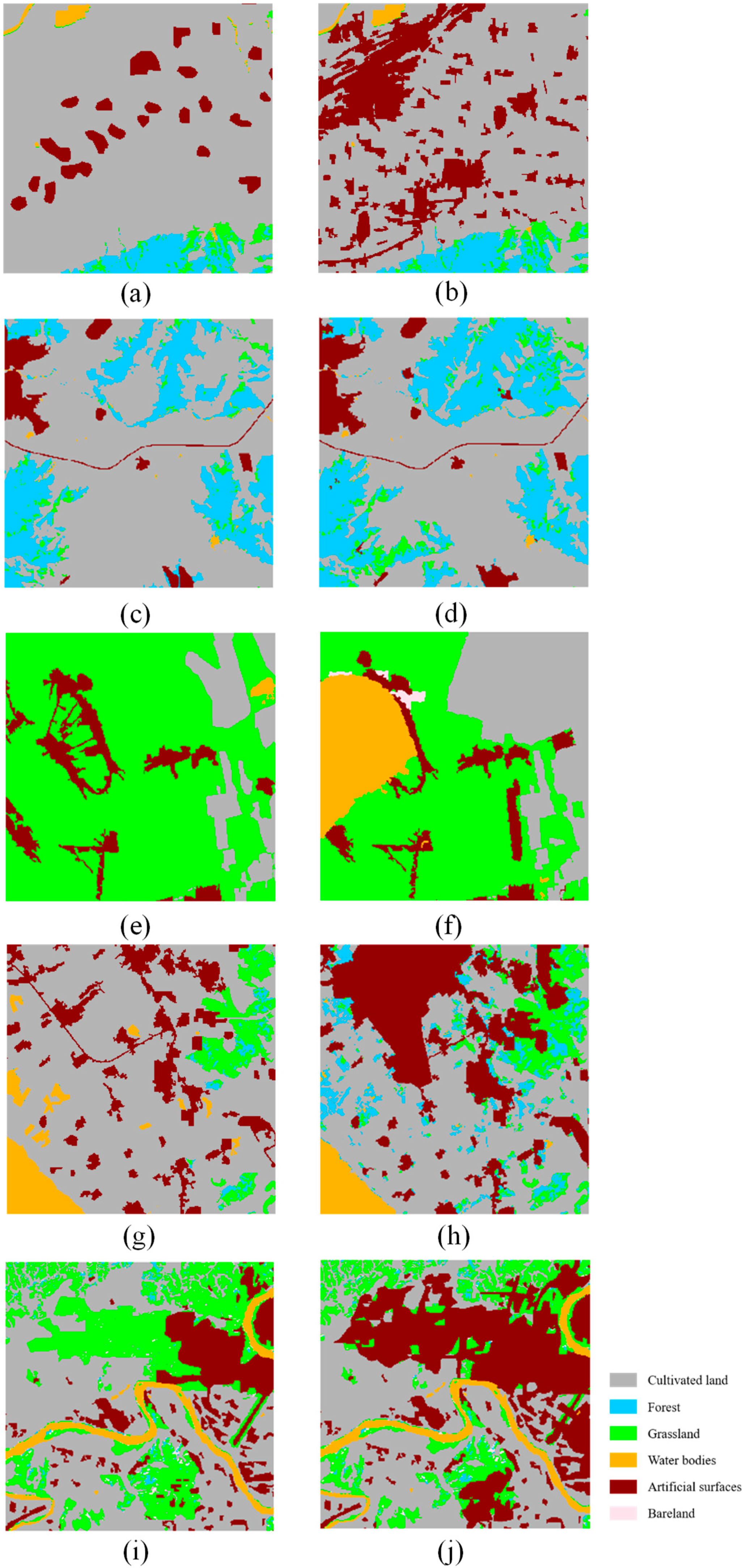
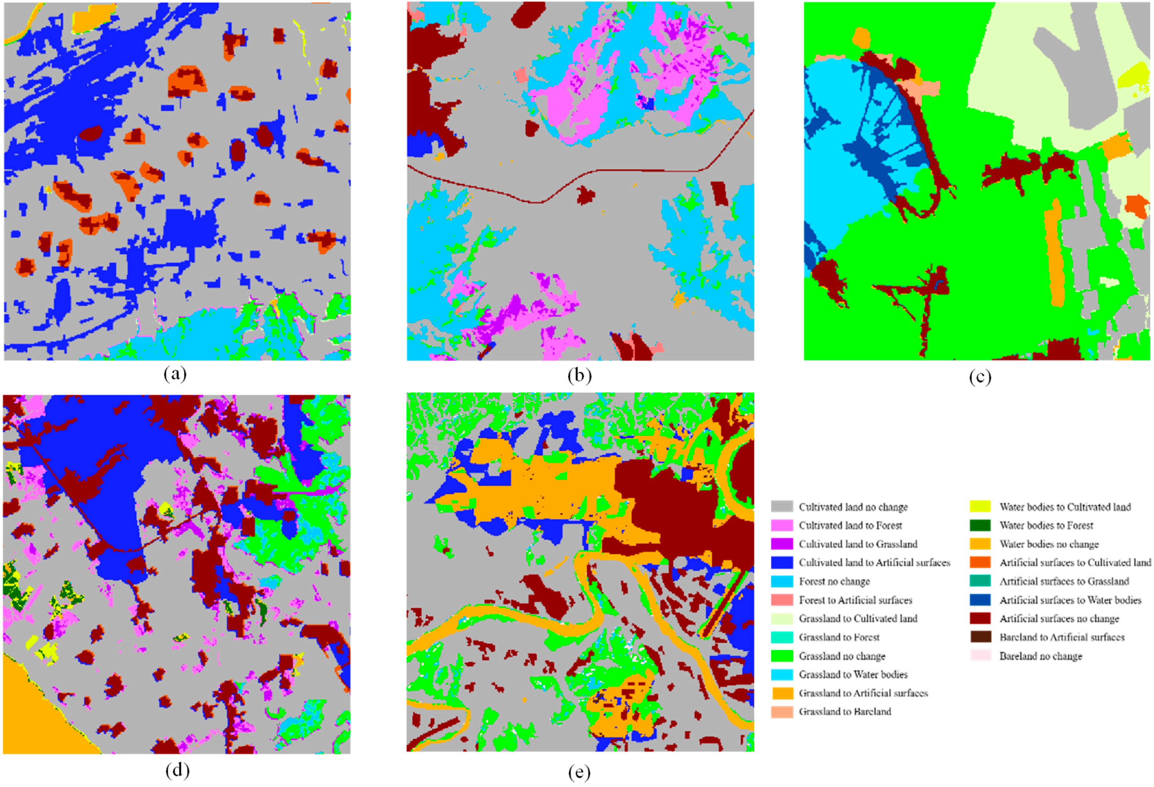
In production of GlobeLand30 2000 and 2010 land-cover, single-date classifications were run independently on source images, although inconsistencies between 2000 and 2010 cover type labelings were checked and corrected (if possible) via spectrally derived change detection [5]. The latter (change detection-based map updating) is likely only effective for homogeneous pixel segments of relatively large areal extents. Thus, when using maps generated from independent classifications for change analyses as for GlobeLand30 products, post-processing is necessary. In this research, for each of the five study sites, the two single-date classification maps (Figure 2) were compared to create a change map with specific “from-to” change information. These land-cover change maps were generated after deleting and re-classifying some non-existing and unlikely change categories (Figure 3).
As mentioned in the introductory section, reference data are required for mapping per-pixel accuracy. They are usually collected from independent sources of higher accuracy (e.g., fine spatial resolution images) through spatial sampling. In Zhang et al. [31], 11 training samples (which refer to reference samples for local accuracy model-building rather than those for training image classifiers) of equal size but with differing configurations of collocated versus non-collocated sample pixels for individual study sites were collected. They are of equal sizes (630 pixels, single-date, corresponding to a sampling intensity of 0.7%), following StRS design. Strata were defined based on “from-to” classes in individual change maps. In this study, we considered only five of the 11 training sample configurations [31] for each of the study sites to reflect the goal of this research: to handle sample configurations 0 through 4, which have entirely or largely non-collocated data (direct methods would be preferred when sufficient collocated sample data are available, as discussed in [31]). The training samples used for this research are summarized in Table 2: configuration 0 contains non-collocated data only (630 sample pixels), while for configuration 1–4 there are 567, 504, 441, and 378 non-collocated sample pixels, respectively. For comparing the performance of the proposed method relative to alternative methods, we used an independent set of 630 collocated bi-temporal reference sample pixels (called validation sample or model-testing sample) collected for each of the study sites [31]. It was collected following simple random sampling (SRS) design.
It would be better to test the proposed method with more experimental datasets if possible. The difficulty to obtain more datasets for this research lies in the following. For change-classification accuracy analyses, we need to have change maps showing some real changes. Moreover, reference data that are in close (if not perfect) temporal proximity of the maps being assessed are required. There seem to be no suitable land-cover datasets over China other than the GlobeLand30 map datasets, which are, however, available only for 2000 and 2010, while 2015 land-cover product is not yet released, meaning it is not feasible to do model validation over more sites and/or across multiple time points. The aforementioned land-cover datasets (both maps and reference samples) at two time points for five sites were what we could furnish in reasonable amount of time to test PXCOV [31]. We believe it was acceptable to use a subset (sample configurations) of the datasets for this research as a compromise between statistical rigorousness and practical feasibility.

2.2. Methods

PXCOV constitutes a theoretically sound method for estimating probabilities of correct change-classification by combining probabilities of correct single-date classifications with adjustment for temporal correlation between them (bi-temporal classification correctness). It supports adaptive use of all sample data available regardless of their being collocated or not [31]. The formula for PXCOV is:
π 1 + 2 ( x 0 ) = π 1 ( x 0 ) π 2 ( x 0 ) + cov I 1 I 2 ( x 0 , x 0 )
where π 1 + 2 ( x 0 ) is the probability of correct change-classification at a location x 0 , π 1 ( x 0 ) and π 2 ( x 0 ) π 2 ( x 0 ) are pixel x 0 ’s probabilities of correct classification at time 1 and time 2, respectively, which may be predicted individually using logistic regression [31], and cov I 1 I 2 ( x 0 , x 0 ) represents cross-covariance of classification correctness at times 1 and 2. Clearly, PXCOV is reduced to method Product when assuming cov I 1 I 2 ( x 0 , x 0 )   =   0 , although this is unlikely to be true, as classification correctness is often temporally correlated.
The key to practical applications of PXCOV lies in estimation of temporal correlation between bi-temporal accuracies. Results obtained by Zhang et al. [31] indicate non-stationarity in temporal correlation, with no-change pixels showing stronger positive temporal correlation, while change pixels exhibit much weaker temporal correlation. In Zhang et al. [31], sample pixels were thus sensibly stratified into no-change and change strata for estimating temporal correlation either through cross-validation cokriging (for sample containing non-collocated data only) or by direct estimation based on collocated sample data if available.
We can make things simpler by stratified approximation of temporal correlation between mono-temporal classification correctness. Specifically, simplification can be achieved by assuming maximum (1.0) and minimum (0.0) correlation over no-change stratum and change stratum, respectively, thus circumventing the complicated process of estimating cross-correlation through cross-validation cokriging with largely non-collocated sample data. This constitutes an approximate yet reasonably accurate alternative solution to PXCOV.
For change pixels where zero cross-correlation is assumed, PXCOV is reduced to a multiplication operator (i.e., product rule, thus named Product in this paper and in Zhang et al. [31]), as discussed concerning Equation (1) above. For no-change pixels where maximum correlation is assumed, synthesis of mono-temporal classification accuracies is basically a minimum operator for probabilities of a pixel being correctly classified at times 1 and 2). Thus, we may compute the probability of pixel x 0 being correctly classified (into a “from-to” class) as:
π 1 + 2 ( x 0 )   =   min ( π 1 ( x 0 ) , π 2 ( x 0 ) )
where π 1 ( x 0 ) and π 2 ( x 0 ) may again be predicted individually using logistic regression as described in Zhang et al. [31] and later in this section. The minimum operator in Equation (2) resembles fuzzy minimum operator, which is widely used in the context of fuzzy sets and synthesis of fuzzy membership values [44,45]. For example, minimum operator was used by Binaghi et al. [43] and Pontius and Cheuk [42] for assessing accuracies of soft classifications. Moreover, “fuzzy” as a label makes more intuitive sense in the context of local accuracy predictions, given the inherent uncertainty in quantifying change-classification accuracies from mono-temporal classification accuracies which are themselves estimated from empirical models (thus subject to uncertainty). Therefore, the minimum operator in Equation (2) is referred to as method Fuzzy. For a typical change map depicting both no-change and change classes, the proposed method applies Fuzzy and Product adaptively and is thus named Fuzzy+Product (meaning combined use of Fuzzy and Product).
A flowchart for the proposed composite method Fuzzy+Product is provided in Figure 4. As shown in Figure 4, single-date local accuracies are predicted using sample data pertaining to single-date classification correctness. These accuracy predictions are combined for estimating local accuracies in change-classification: minimum values of predicted probabilities of correct classifications in single-date maps are used as estimates of joint probabilities of correct classification over no-change pixels, while multiplication operator for joint probabilities of correct classification over change pixels where class-conditional independence is usually assumed.
As mentioned above, for predictions of per-pixel probabilities of correct classification for single-date maps, logistic regression modeling is performed based on (model) training sample data, using map class occurrence pattern indices as explanatory variables. These pattern indices include land-cover class (class) and several landscape characteristics indices computed over different window sizes (3 × 3, 7 × 7, 11 × 11, 15 × 15, 17 × 17, 19 × 19, and 21 × 21 pixels), such as heterogeneity (het), homogeneity (hom), dominance (dmg), contagion (con), and entropy (ent). Class is coded by binary variables to indicate the presence of one of the candidate classes in single-date maps. Heterogeneity (het) refers to the number of different classes in the moving window. Homogeneity (hom) indicates the number of pixels with the same class label as the center pixel in the moving window. Dominance (dmg) represents the deviation value between landscape diversity and maximum diversity in the moving window. Contagion (con) is the extent to which different patch types are aggregated or clumped. Entropy (ent) indicates the average uncertainty of class occurrences [31]. The significant explanatory for single-date classification maps (time 1 and time 2) at individual study sites can be identified, following model selection procedures [21,31,46].
To test the performance of the proposed method (i.e., Fuzzy+Product) relative to alternative methods (i.e., PXCOV, Fuzzy, and Product) for mapping change-classification accuracies, area under the receiver operating characteristic curve (AUC) can be used. As recommend in the literatures, AUCs measure the discriminatory powers of classifiers (e.g., alternative accuracy predictors discussed in the paper) and are often used for prediction-model comparisons, with greater AUC values indicating more accurate predictions [29,47,48]. AUC-based statistical testing needs to be performed to determine if one method is significantly more (or less) accurate than another or if there is no significant difference between a pair of methods’ performance. For this research, the related computation concerning AUC values and statistical testing of difference between AUC values were carried out using R package pROC [48].

3. Results

3.1. Model Fitting and Predictions

The optimal model containing the largest number of significant explanatory variables for each single-date classification maps with samples of different configurations at the five study sites are shown in Table 3, which is excerpted from Zhang et al. [31]. The numbers after explanatory variables (except for class) shown in Table 3 are sizes of the moving windows surrounding a sample pixel.
The optimal models identified for mono-temporal classification maps allowed for computing probabilities of correct change-categorization at validation sample pixels by methods Fuzzy, Product, and Fuzzy+Product straightforwardly. The estimated probabilities were then compared with reference data for performance evaluations, as described in Section 3.2.
For PXCOV, depending on availability of collocated sample data, there are two options: one is cross-validation co-kriging when collocated sample data are not available or insufficient, the other is direct estimation using collocated sample data when available [31]. Note that sample pixels need to be stratified into change and no-change strata for temporal correlation estimation in PXCOV, as described in Zhang et al. [31]. Results are reported in Table 4, where estimates of temporal correlation were actually obtained through cross-validation cokriging (configuration 0) and collocated sample data (configurations 1–4), respectively.
As shown in Table 4, temporal correlation is generally large for no-change pixels (up to 1.0) but quite small for change pixels, confirming the appropriateness of using the minimum and multiplication operators for no-change stratum and change stratum, respectively. Exceptions are with study site CE (configuration 1, change stratum; configuration 3, no-change stratum) and site SE (configuration 0, no-change stratum), as shown in Table 4. This may be due to special landscape patterns depicted by the relevant maps and indicates potential problems in estimating temporal correlation either by computation (cross-validation cokriging) or based on modest amount of collocated sample data.
As for other methods tested in this research, estimated probabilities at validation sample pixels by PXCOV were used for performance evaluations. This is described in Section 3.2.
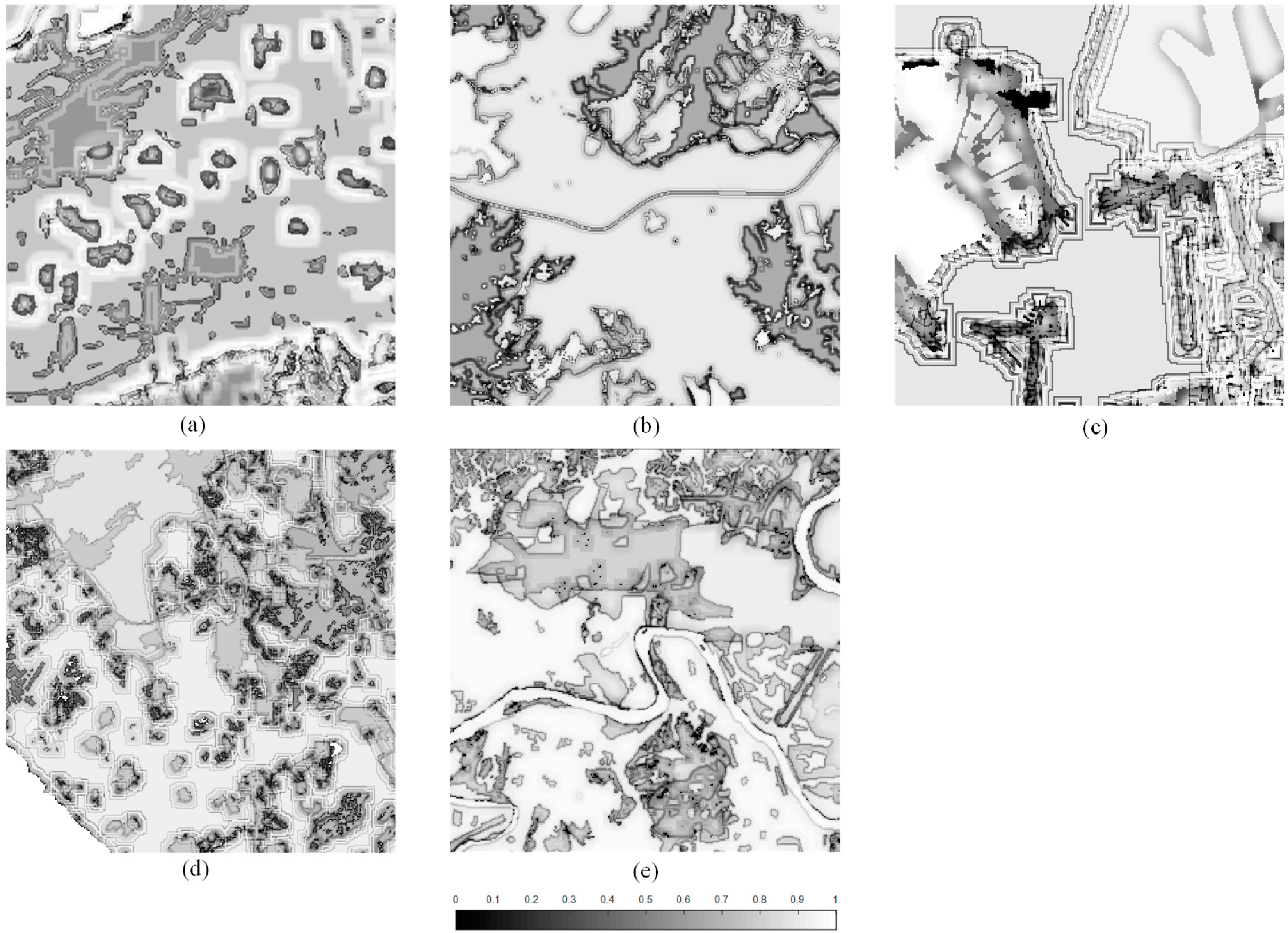
The probability maps of correct change categorization could be generated based on different sample configurations at five study sites. An example is given in Figure 5a–e, showing the accuracy surfaces derived from Fuzzy+Product based on samples of configuration 0 at five study sites. Figure 5a–e reveal that the greater accuracy is predicted for persistent classes, in particular, water bodies (no-change) and cultivated land (no-change). This can be explained by their easy identification from remotely sensed images. Additionally, this reflects the facts that greater accuracies in single-date classifications (e.g., certain single-date static cover types, such as water bodies) tend to lead to greater accuracies in change-classification (e.g., corresponding persistence types) and that class is a significant explanatory variable for logistic regression modeling concerning probabilities of correct (single-date) classifications.

3.2. Performance Evaluations

As mentioned towards the end of Section 2.2, AUC (area under the receiver operating characteristic curve) was used to evaluate performances of different methods for mapping change classification accuracies at individual study sites. Based on an independent set of 630 collocated bi-temporal validation sample pixels collected for each of the study sites, AUCs values of different methods based on different configuration samples were computed using the R package pROC [48], as shown in Table 5. Almost all model predictions shown in Table 5 are reasonable (with AUC measures exceeding 0.70). There are obvious variations in AUC measures across different study sites and by different methods, although those among sample configurations are decreased.
AUC-based statistical testing was performed to examine whether there exist significant differences between a pair of methods’ performance, leading to results shown in Table 6. R package pROC [48] was also used to perform significance tests.
Firstly, as shown in Table 5 and Table 6, the proposed method is significantly more accurate than Fuzzy and Product in general. Their differences in AUC values are quite large for some cases (e.g., those at site CE), although they become small and insignificant in other cases, in particular, sites NE and NW, for most sample configurations.
Secondly, as shown in Table 6, there are no significant differences between the results obtained by Fuzzy+Product and PXCOV at all study sites. Their differences in AUC values are quite small, although they become large at site CE. We elaborate on the evaluation results below.
As shown in Table 6, some greater AUC differences were tested as being insignificant, while some smaller ones registered significance. This is because Z statistic used in significance testing depends not only on the magnitude of differences but also their variance. As the variance depends on the covariance of the ROC curves (var(y1 − y2) = var(y1) + var(y2) − 2cov(y1,y2)), strongly (positively) correlated ROC curves can have similar AUC values and still be significantly different (since Z = (y1 − y2)/[var(y1 − y2)] 1/2) [48,49,50,51,52].
Consider the varying AUC values at the five study sites. Our understanding is that performances (indicated by AUC values) of alternative indirect methods reflect the predictive accuracies of the models they are based on. For change maps, AUC values are affected by the predictive accuracies of logistic models for single-date classification maps, the accuracies in cross-correlation estimation, and those in differentiation between true change versus true no-change pixels. As logistic models use a selection of map class occurrence pattern indices as explanatory variables, predictive accuracies of single-date classifications are clearly dependent on the peculiarity of the landscape mapped at a site. Thus, site CE’s higher AUC value reflects the collective effects of relatively higher accuracies in single-date classification accuracy predictions (due to site map class pattern), cross-correlation estimation, and differentiation of change versus no-change pixels than at other sites.
As for the greater differences in AUC values at site CE, our understanding is that alternative methods’ differing performances are probably best manifested there. All other factors being the same, accuracy in estimating cross-correlation may be a major contributor to the differences: cross-correlation is estimated based on sample data in PXCOV but approximated in Fuzzy+Product. The relationships between relative performances of alternative methods and the aforementioned possible factors certainly merit consideration.

4. Discussion

The proposed method (i.e., Fuzzy+Product) has been shown to be more accurate than both Fuzzy and Product in general, while being comparable to PXCOV (which was previously recommended for the mapping of local accuracies in change-classifications when collocated data are not available or insufficient). This suggests that we should use Fuzzy+Product for balance between simplicity and accuracy, given its being much easier to use than PXCOV.
Below, we give some retrospective and prospective views on this research. In particular, the proposed method’s advantages and disadvantages relative to its major competitor, PXCOV, are assessed in the light of what were revealed in this research. Prospectively, future work on Fuzzy+Product’s extensibilities to accuracy characterization in multi-temporal change analyses and fuzzy/fractional change-classification is discussed, while that on linking up local and global accuracy analyses (including area estimation) is briefly elaborated on where locally constrained error matrices [22] play an essential role.

4.1. Fuzzy+Product versus PXCOV

Consider limitations of PXCOV, Fuzzy+Product’s major competitor, in terms of prediction accuracy (i.e., AUC reported in Section 3.2). Apart from inaccuracy in single-date model predictions, as with all methods tested in this research, inaccuracy in temporal correlation estimation has a direct effect on PXCOV. Although not reported, we explored ways to improve estimation of temporal correlation for possible enhancement of PXCOV. Emphasis was placed upon stratified estimation of temporal correlation (assuming availability of reasonable amount of collocated sample data) with strata being specific persistence cover types and one single stratum of change. Results showed that stratified estimation does not improve predictions. This is probably due to much smaller sample sizes in individual strata. Increasing sample sizes of collocated data would be out of the question for PXCOV, as it has advantages over direct methods only when data available are largely non-collocated (direct methods would be preferred when given sufficient collocated data). At a fundamental level, predicting joint probabilities of correct classification through synthesis of single-date probabilities by PXCOV is a kind of approximation after all, and thus, subject to uncertainty. Moreover, estimation of temporal correlation by cross-validation cokriging would become extremely complicated and technically infeasible when dealing with accuracy analyses in multi-temporal change categorization (see discussion below). In addition, uncertainty in estimation of temporal correlation (if it is possible to do so at all) is likely to propagate quickly in accuracy analyses in the context of long-term land-cover monitoring, reducing theoretical benefits of using PXCOV. These argue for Fuzzy+Product being a sensible and cost-effective alternative to PXCOV.
The performance of Fuzzy+Product depends on the accuracy with which local accuracies in single-date classification maps are estimated and is limited by the inaccuracy due to approximating temporal correlation with 1.0 and 0.0 for no-change stratum and change stratum, respectively. As the maps being analyzed are subject to misclassification errors, stratification of unsampled pixels into change or no-change stratum is subject to error. The net result is that local accuracy predictions by Fuzzy+Product suffer from propagation of various errors, as with change detection based on post-classification comparisons. This should be noted when interpreting and using results obtained with Fuzzy+Product. Moreover, the inherently uncertain nature of accuracy predictions actually indicates the merits of fuzzy logic-based approaches [25,43,53,54,55,56,57] in evaluating and analyzing change-classification accuracies, as is further discussed towards the end of Section 4.2.
Fuzzy+Product and all alternative methods considered in this paper are applied in the ways they are designed regardless of how change maps are derived (i.e., whether from independent classifications of mono-temporal images or spectrally based change detection [4]). For Fuzzy+Product, in particular, the assumption about maximum and minimum cross-correlation over no-change and change pixels, respectively, is made regardless how the change maps are produced. However, it makes sense to revisit that assumption by investigating how it is affected by the ways change maps are produced (i.e., independent classifications versus change detection followed by map updating). It is asserted that independent classifications tend to induce minimum correlation even over no-change pixels (which explains why Product’s performance is not inferior to that of PXCOV by a large margin of AUC values), while change detection followed by change-classification likely makes maximum correlation more plausible (not only over no-change pixels but also change pixels). This is definitely a topic worth exploring in the future.

4.2. Extensions of Fuzzy+Product to Multi-Temporal Change Analyses and Fuzzy/Fractional Classifications

Further research should be pursued on topics related to or as an extension of the work reported in this paper. One of them is the extension of the proposed method from a bi-temporal context to a multi-temporal one. With more time points considered in multi-temporal change analyses [7,8,16], there is an increase of the number of “from-to” classes, while the sample data are always limited. In such cases, the Fuzzy+Product method will be very valuable as non-collocated sample data become more a norm than an exception, although current NLCD land-cover product validation are predominately based on collocated reference data [14]. For example, local accuracy characterization in change analyses over long time series and/or across arbitrary multiple time intervals would be well supported by Fuzzy+Product. We can do this cumulatively and progressively as time-specific new reference data and additional maps are incorporated for accuracy analyses. Fuzzy+Product’s easy extension to multi-temporal applications originates from its simplicity: minimum and multiplication operators are applied straightforwardly across multiple time points. In contrast, complicated geostatistical modeling is involved in use of PXCOV (even in a bi-temporal setting), which may not be able to provide accuracy predictions in a multi-temporal setting by simple applications of two-point variogram modeling and cross-validation co-kriging.
We have to admit that when working on PXCOV previously it was difficult to acquire real datasets (both maps to be assessed and corresponding reference sample data) suitable for bi-temporal change product validation, let alone those for multi-temporal applications, as mentioned in Section 2.1. The situation has not improved yet since this research was undertaken. On the other hand, use of simulated datasets is cautioned since simulated data may not be able to reflect misclassification patterns as complex and unique as in real datasets. Thus, we were not able to test the proposed method with real multi-temporal datasets, although this is certainly a research topic worth pursuing in the future.
It should be noted that Fuzzy+Product may not be directly used for mapping local accuracies in soft or fuzzy classifications of land-cover change per se, as the underlying logic for fuzzy classification is fuzzy sets, while discussion of land-cover and change in this research is based on crisp sets. Proper methods are discussed by authors including Khatami et al. [25]. However, if fuzzy accuracy measures (i.e., fuzzy membership values for the class of pixels being correctly classified) are treated as probabilistic ones for single-date and change classifications and we are willing to relax the probabilistic assumptions underlying this research, Fuzzy+Product may be applied to compute accuracies in a change map based on single-date classification accuracies at pixel level (and the change map itself for computing map class occurrence pattern indices). Similarly, for fractional land-cover maps (or percent cover maps), if areal proportions of candidate land-cover classes within a pixel are used as surrogates of probabilities of correctly classifying a pixel as the corresponding classes and if we consider only the primary classes (which have the maximum proportions in individual pixels, with the maximum proportions being used as probabilistic measures of accuracy), we may apply the proposed method to predict class proportions (“from-to” classes, to be exact), which can be viewed as accuracy estimates for “from-to” class labels on change maps derived from single-date fractional cover maps. Following this reasoning, Fuzzy+Product’s extension to multi-temporal fractional maps would be straightforward. Nevertheless, further work is required if both primary and alternate class labels are considered for assessing class agreement in local change-classification accuracy mapping.

4.3. Accuracy Characterization: from Local back to Global

With maps of local accuracies created from the proposed method (e.g., those in Figure 5), it is definitely interesting to find out if the accuracy of the entire map can be derived from the local versions. However, the answer is not so straightforward, as explained below.
As this research focuses on the settings where reference sample data are largely non-collocated, it would be problematic to undertake global accuracy assessment (for an entire map) directly based on error matrices that would require availability of sufficient collocated sample data. The method proposed in this paper provides a possible solution for this. The predicted per-pixel change-classification accuracy may be summed over the whole map and averaged to give a coarse approximation of the overall accuracy (OA); even for a single-date classification map, the local accuracy predictions can only be used to derive a coarse approximation of OA. A fix would be to apply the so-called model-assisted methods as discussed in McRoberts et al. [58]. There have been many research efforts applying model-assisted and other related methods in the literature (e.g., 38, 59–62). It is important to note that estimators need to account for specific sampling design (e.g., stratified random sampling (StRS) versus simple random sampling (SRS)).
For user’s and producer’s accuracies (i.e., UA and PA) assessed of the entire map, the aforementioned local accuracy predictions are of little use. Adapted use of the method (Fuzzy+Product) for localized UA and PA followed by bias-corrections through model-assisted methods may be usefully explored. However, unless SRS sample data are used, the local-to-global transfers of UA and PA are not direct or linear, let alone estimation of their uncertainties.
We need to revisit the design-based and model-based inference approaches [58,59,60,61,62]. This is to construct error matrices, with their cell proportions (for combinations of map class i and reference class j) properly estimated based on sample weighting. Accuracy measures including OA, UA, and PA can be easily derived from properly estimated cell probabilities. Area estimates from maps may also be corrected based on the aforementioned error matrices, with confidence intervals evaluated, as by-products of standard accuracy assessments [63,64]. This prompts for predictions of localized error matrices (with cell proportions estimated properly) [18,28]. They (error matrices) may then be analyzed using model-assisted approaches to derive globally aggregated error matrices, which can in turn be used to derive accuracy measures (including OA, UA, and PA) for the entire map and their confidence intervals. Areal estimate corrections may also be done based on globally summarized error matrices. Having said so, we are aware that there exist numerous issues for the aforementioned local-to-global accuracy characterization in change maps using largely non-collocated reference sample data.

5. Conclusions

This paper has tested a simple extension method (i.e., Fuzzy+Product) to PXCOV for mapping per-pixel change-classification accuracies, when sample data are non-collocated or mostly so (typically being the case when reference data for mono-temporal classifications are collected independently). By this method, minimum operator (labeled Fuzzy as it is similar to fuzzy set “min” operator) is applied over no-change pixels’ stratum: the minimum values of predicted probabilities of correct classifications in single-date maps are used as approximation of joint probabilities of correct change-classifications with the understanding that temporal correlation over persistence classes is usually strong. For change pixels’ stratum, multiplication operator (method Product) is applied by assuming zero temporal correlation (as it is usually very weak over change pixels). Both operators are applied over their corresponding strata regardless of sample configurations concerned. Empirical results confirmed that Fuzzy+Product is more accurate than both Fuzzy and Product in general and that there are no significant differences between Fuzzy+Product and PXCOV (which is hardly more accurate but involves use of a complicated procedure of cross-validation cokriging) in terms of AUC. This indicates that Method Fuzzy+Product offers a simpler but reasonably accurate alternative to PXCOV. Future research and developments on refining it, extending it to accuracy characterization in multi-temporal change analyses and fuzzy/fractional change-classifications, and utilizing it for bridging the gap between local and global change accuracy analyses when reference sample data are largely non-collocated should be promoted.

Author Contributions

Y.M. and J.Z. proposed the study, designed and carried out data analyses, and contributed to manuscript writing and revision. W.Z. contributed to acquisition and analyses of sample data. F.L. helped with reference data sources.

Funding

This research was funded by the National Social Science Foundation of China (grant no. 19CSH004), the National Natural Science Foundation of China (grant no. 41471375), the General Financial Grant from China Postdoctoral Science Foundation (grant no. 2019M662723), and the Beijing Key Laboratory of Urban Spatial Information Engineering (grant no. 2019101).

Acknowledgments

We thank our anonymous reviewers for their comments and suggestions. Roger Kirby (retiree from The University of Edinburgh, Scotland), Michael F. Goodchild (Emeritus Professor of Geography at the University of California, Santa Barbara), and Jun Chen (newly elected Academician, Chinese Academy of Engineering) have provided long-term advice about spatial uncertainty for J.Z., the corresponding author.

Conflicts of Interest

The authors declare no conflict of interest.

References

  1. Lambin, E.F.; Turner, B.L.; Geist, H.J.; Agbola, S.B.; Angelsen, A.; Bruce, J.W.; Folke, C. The causes of land-use and land-cover change: Moving beyond the myths. Glob. Environ. Chang. 2001, 11, 261–269. [Google Scholar] [CrossRef]
  2. See, L.; Schepaschenko, D.; Lesiv, M.; Mccallum, I.; Fritz, S.; Comber, A.; Maus, V. Building a hybrid land cover map with crowdsourcing and geographically weighted regression. ISPRS J. Photogramm. Remote Sens. 2015, 103, 48–56. [Google Scholar] [CrossRef]
  3. Friedl, M.A.; Sullamenashe, D.; Tan, B.; Schneider, A.; Ramankutty, N.; Sibley, A.; Huang, X.M. MODIS collection 5 global land cover: Algorithm refinements and characterization of new datasets. Remote Sens. Environ. 2010, 114, 168–182. [Google Scholar] [CrossRef]
  4. Hansen, M.C.; Loveland, T.R. A review of large area monitoring of land cover change using Landsat data. Remote Sens. Environ. 2012, 122, 66–74. [Google Scholar] [CrossRef]
  5. Chen, J.; Chen, J.; Liao, A.; Cao, X.; Chen, L.; Chen, X.; He, C.; Han, G.; Peng, S.; Lu, M.; et al. Globel land cover mapping at 30m resolution: A POK-based operational approach. ISPRS J. Photogramm. Remote Sens. 2015, 103, 7–27. [Google Scholar] [CrossRef]
  6. Yang, L.; Jin, S.; Danielson, P.; Homer, C.; Gass, L.; Bender, S.M.; Fry, J. A new generation of the United States national land cover database: Requirements, research priorities, design, and implementation strategies. ISPRS J. Photogramm. Remote Sens. 2018, 146, 108–123. [Google Scholar] [CrossRef]
  7. Tsutsumida, N.; Comber, A.J. Measures of spatio-temporal accuracy for time series land cover data. Int. J. Appl. Earth Obs. Geoinf. 2015, 41, 46–55. [Google Scholar] [CrossRef]
  8. Hermosilla, T.; Wulder, M.A.; White, J.C.; Coops, N.C.; Hobart, G.W. Disturbance-informed annual land cover classification maps of Canada’s forested ecosystems for a 29-year Landsat time series. Can. J. Remote Sens. 2018, 44, 67–87. [Google Scholar] [CrossRef]
  9. Hayes, D.J.; Cohen, W.B.; Sader, S.A.; Irwin, D.E. Estimating proportional change in forest cover as a continuous variable from multi-year MODIS data. Remote Sens. Environ. 2008, 112, 735–749. [Google Scholar] [CrossRef]
  10. Chi, Z.; Chen, Y.; Lu, D. Detecting fractional land-cover change in arid and semiarid urban landscapes with multitemporal Landsat Thematic mapper imagery. GISci. Remote Sens. 2015, 52, 700–722. [Google Scholar]
  11. Rigge, M.; Shi, H.; Homer, C.; Danielson, P.; Granneman, B. Long-term trajectories of fractional component change in the Northern Great Basin, USA. Ecosphere 2019, 10, e02762. [Google Scholar] [CrossRef]
  12. Congalton, R.G.; Gu, J.Y.; Yadav, K.; Thenkabail, P.; Ozdogan, M. Global land cover mapping: A review and uncertainty analysis. Remote Sens. 2014, 6, 12070–12093. [Google Scholar] [CrossRef]
  13. White, M.A.; Shaw, J.D.; Ramsey, R.D. Accuracy assessment of the vegetation continuous field tree cover product using 3954 ground plots in the southwestern USA. Int. J. Remote Sens. 2005, 26, 2699–2704. [Google Scholar] [CrossRef]
  14. Wickham, J.D.; Stehman, S.V.; Gass, L.; Dewitz, J.; Fry, J.A.; Wade, T.G. Accuracy assessment of NLCD 2006 land cover and impervious surface. Remote Sens. Environ. 2013, 130, 294–304. [Google Scholar] [CrossRef]
  15. Tsendbazar, N.E.; Bruin, S.D.; Fritz, S.; Herold, M. Spatial accuracy assessment and integration of global land cover datasets. Remote Sens. 2015, 7, 15804–15821. [Google Scholar] [CrossRef]
  16. Leyk, S.; Uhl, J.H.; Balk, D.; Jones, B. Assessing the accuracy of multi-temporal built-up land layers across rural-urban trajectories in the United States. Remote Sens. Environ. 2018, 204, 898–917. [Google Scholar] [CrossRef]
  17. Stehman, S.V.; Foody, G.M. Key issues in rigorous accuracy assessment of land cover products. Remote Sens. Environ. 2019, 231, 111199. [Google Scholar] [CrossRef]
  18. Comber, A.J. Geographically weighted methods for estimating local surfaces of overall, user and producer accuracies. Remote Sens. Lett. 2013, 4, 373–380. [Google Scholar] [CrossRef]
  19. Steele, B.M.; Winne, J.C.; Redmond, R.L. Estimation and mapping of misclassification probabilities for thematic land cover maps. Remote Sens. Environ. 1998, 66, 192–202. [Google Scholar] [CrossRef]
  20. Smith, J.H.; Stehman, S.V.; Wickham, J.D.; Yang, L. Effects of landscape characteristics on land-cover class accuracy. Remote Sens. Environ. 2003, 84, 342–349. [Google Scholar] [CrossRef]
  21. Van Oort, P.A.J.; Bregt, A.K.; de Bruin, S.; de Wit, A.J.W.; Stein, A. Spatial variability in classification accuracy of agricultural crops in the Dutch national land-cover database. Int. J. Geogr. Inf. Sci. 2004, 18, 611–626. [Google Scholar] [CrossRef]
  22. Foody, G.M. Local characterization of thematic classification accuracy through spatially constrained confusion matrices. Int. J. Remote Sens. 2005, 26, 1217–1228. [Google Scholar] [CrossRef]
  23. Burnicki, A.C. Modeling the probability of misclassification in a map of land cover change. Photogramm. Eng. Remote Sens. 2011, 77, 39–49. [Google Scholar] [CrossRef]
  24. Park, N.W.; Kyriakidis, P.; Hong, S.Y. Spatial estimation of classification accuracy using indicator Kriging with an image-derived ambiguity index. Remote Sens. 2016, 8, 320. [Google Scholar] [CrossRef]
  25. Khatami, R.; Mountrakis, G.; Stehman, S.V. Mapping per-pixel predicted accuracy of classified remote sensing images. Remote Sens. Environ. 2017, 191, 156–167. [Google Scholar] [CrossRef]
  26. Yang, Y.; Xiao, P.; Feng, X.; Li, H. Accuracy assessment of seven global land cover datasets over China. ISPRS J. Photogramm. Remote Sens. 2017, 125, 156–173. [Google Scholar] [CrossRef]
  27. Wickham, J.; Stehman, S.V.; Homer, C.G. Spatial patterns of the United States National Land Cover Dataset (NLCD) land-cover change thematic accuracy (2001–2011). Int. J. Remote Sens. 2018, 39, 1729–1743. [Google Scholar] [CrossRef]
  28. Comber, A.; Brunsdon, C.; Charlton, M.; Harris, P. Geographically weighted correspondence matrices for local error reporting and change analyses: Mapping the spatial distribution of errors and change. Remote Sens. Lett. 2017, 8, 234–243. [Google Scholar] [CrossRef]
  29. Khatami, R.; Mountrakis, G.; Stehman, S.V. Predicting individual pixel error in remote sensing soft classification. Remote Sens. Environ. 2017, 199, 401–414. [Google Scholar] [CrossRef]
  30. Zhang, J.; Yang, W.; Zhang, W.; Wang, Y.; Liu, D.; Xiu, Y. An explorative study on estimating local accuracies in land-cover information using logistic regression and class-heterogeneity-stratified data. Remote Sens. 2018, 10, 21. [Google Scholar] [CrossRef]
  31. Zhang, J.; Zhang, W.; Mei, Y.; Yang, W. Geostatistical characterization of local accuracies in remotely sensed land cover change categorization with complexly configured reference samples. Remote Sens. Environ. 2019, 223, 63–81. [Google Scholar] [CrossRef]
  32. Bey, A.; Sánchezpaus Díaz, A.; Maniatis, D.; Marchi, G.; Mollicone, D.; Ricci, S.; Rezende, M. Collect earth: Land use and land cover assessment through augmented visual interpretation. Remote Sens. 2016, 8, 807. [Google Scholar] [CrossRef] [Green Version]
  33. Cohen, W.B.; Yang, Z.; Kennedy, R. Detecting trends in forest disturbance and recovery using yearly Landsat time series: 2. TimeSync-tools for calibration and validation. Remote Sens. Environ. 2010, 114, 2911–2924. [Google Scholar] [CrossRef]
  34. Lark, R.M.; Bellamy, P.H.; Rawlins, B.G. Spatio-temporal variability of some metal concentrations in the soil of eastern England, and implications for soil monitoring. Geoderma 2006, 133, 363–379. [Google Scholar] [CrossRef]
  35. Fritz, S.; Mccallum, I.; Schill, C.; Perger, C.; See, L.; Schepaschenko, D.; Obersteiner, M. Geo-Wiki: An online platform for improving global land cover. Environ. Model. Softw. 2012, 31, 110–123. [Google Scholar] [CrossRef]
  36. Stehman, S.V.; Olofsson, P.; Woodcock, C.E.; Herold, M.; Friedl, M.A. A global land-cover validation data set, II: Augmenting a stratified sampling design to estimate accuracy by region and land-cover class. Int. J. Remote Sens. 2012, 33, 6975–6993. [Google Scholar] [CrossRef]
  37. Olofsson, P.; Foody, G.M.; Herold, M.; Stehman, S.V.; Woodcock, C.E.; Wulder, M.A. Good practices for estimating area and assessing accuracy of land change. Remote Sens. Environ. 2014, 148, 42–57. [Google Scholar] [CrossRef]
  38. Mcroberts, R.E.; Walters, B.F. Statistical inference for remote sensing-based estimates of net deforestation. Remote Sens. Environ. 2012, 124, 394–401. [Google Scholar] [CrossRef]
  39. Zhang, J.; Mei, Y. Integrating logistic regression and geostatistics for user-oriented and uncertainty-informed accuracy characterization in remotely-sensed land cover change information. ISPRS Int. J. Geo-Inf. 2016, 5, 113. [Google Scholar] [CrossRef] [Green Version]
  40. Overton, W.S.; Stehman, S.V. Desirable design characteristics for long-term monitoring of ecological variables. Environ. Ecol. Stat. 1996, 3, 349–361. [Google Scholar] [CrossRef]
  41. Steele, B.M. Combining multiple classifiers: An application using spatial and remotely sensed information for land cover type mapping. Remote Sens. Environ. 2000, 74, 545–556. [Google Scholar] [CrossRef]
  42. Pontius, R.G.; Cheuk, M.L. A generalized cross-tabulation matrix to compare soft-classified maps at multiple resolutions. Int. J. Geogr. Inf. Sci. 2006, 20, 1–30. [Google Scholar] [CrossRef]
  43. Binaghi, E.; Brivio, P.A.; Ghezzi, P.; Rampini, A. A fuzzy set-based accuracy assessment of soft classification. Pattern Recognit. Lett. 1999, 20, 935–948. [Google Scholar] [CrossRef]
  44. Zadeh, L.A. Fuzzy sets. Inf. Control 1965, 8, 338–353. [Google Scholar] [CrossRef] [Green Version]
  45. Ahlqvist, O. Extending post-classification change detection using semantic similarity metrics to overcome class heterogeneity: A study of 1992 and 2001 U.S. national land cover database changes. Remote Sens. Environ. 2008, 112, 1226–1241. [Google Scholar] [CrossRef]
  46. Smith, J.H.; Stehman, S.V.; Wickham, J.D. Impacts of patch size and land-cover heterogeneity on thematic image classification accuracy. Photogramm. Eng. Remote Sens. 2002, 68, 65–70. [Google Scholar]
  47. Liu, C.; White, M.; Newell, G. Measuring and comparing the accuracy of species distribution models with presence-absence data. Ecography 2011, 34, 232–243. [Google Scholar] [CrossRef]
  48. Robin, X.; Turck, N.; Hainard, A.; Tiberti, N.; Lisacek, F.; Sanchez, J.-C.; Müller, M. pROC: An open-source package for R and S+ to analyze and compare ROC curves. BMC Bioinform. 2011, 12, 77. [Google Scholar] [CrossRef]
  49. DeLong, E.; DeLong, D.; Clarke-Pearson, D. Comparing the areas under two or more correlated receiver operating characteristic curves: A nonparametric approach. Biometrics 1988, 44, 837–845. [Google Scholar] [CrossRef]
  50. Hanley, J.A.; McNeil, B.J. A method of comparing the areas under receiver operating characteristic curves derived from the same cases. Radiology 1983, 148, 839–843. [Google Scholar] [CrossRef] [Green Version]
  51. Venkatraman, E.S. A permutation test to compare receiver operating characteristic curves. Biometrics 2000, 56, 1134–1138. [Google Scholar] [CrossRef] [PubMed]
  52. Venkatraman, E.S.; Begg, C.B. A distribution-free procedure for comparing receiver operating characteristic curves from a paired experiment. Biometrika 1996, 83, 835–848. [Google Scholar] [CrossRef]
  53. Dombi, J. A general class of fuzzy operators, the DeMorgan class of fuzzy operators and fuzziness measures induced by fuzzy operators. Fuzzy Sets Syst. 1982, 8, 149–163. [Google Scholar] [CrossRef]
  54. Fritz, S.; Lee, L. Comparison of land cover maps using fuzzy agreement. Int. J. Geogr. Inf. Sci. 2005, 19, 787–807. [Google Scholar] [CrossRef] [Green Version]
  55. Koch, J.; Jensen, K.H.; Stisen, S. Toward a true spatial model evaluation in distributed hydrological modeling: Kappa statistics, Fuzzy theory, and EOF analysis benchmarked by the human perception and evaluated against a modeling case study. Water Resour. Res. 2015, 51, 1225–1246. [Google Scholar] [CrossRef]
  56. Lowry, J.H.; Ramsey, R.D.; Stoner, L.L.; Kirby, J.; Schulz, K. An Ecological Framework for Evaluating Map Errors Using Fuzzy Sets. Photogramm. Eng. Remote Sens. 2008, 74, 1509–1519. [Google Scholar] [CrossRef]
  57. Hester, D.B.; Nelson, S.A.C.; Cakir, H.I.; Khorram, S.; Cheshire, H. High-resolution land cover change detection based on fuzzy uncertainty analysis and change reasoning. Int. J. Remote Sens. 2010, 31, 455–475. [Google Scholar] [CrossRef]
  58. McRoberts, R.E. Probability- and model-based approaches to inference for proportion forest using satellite imagery as ancillary data. Remote Sens. Environ. 2010, 114, 11017–11025. [Google Scholar] [CrossRef]
  59. Stahl, G.; Saarela, S.; Schnell, S.; Holm, S.; Breidenbach, J.; Healey, S.P.; Patterson, P.L.; Magnussen, S.; Naesset, E.; McRoberts, R.E.; et al. Use of models in large-area forest surveys: Comparing model-assisted, model-based and hybrid estimation. For. Ecosyst. 2016, 3, 5. [Google Scholar] [CrossRef] [Green Version]
  60. Naesset, E.; Orka, H.O.; Solberg, S.; Bollandsas, O.M.; Hansen, E.H.; Mauya, E.; Zahabu, E.; Malimbwi, R.; Chamuya, N.; Olsson, H.; et al. Mapping and estimating forest area and aboveground biomass in miombo woodlands in Tanzania using data from airborne laser scanning. Remote Sens. Environ. 2016, 175, 282–300. [Google Scholar] [CrossRef]
  61. Stahl, G.; Holm, S.; Timothy, G.; Gregoire, T.; Naesset, E.; Nelson, R. Model-based inference for biomass estimation in a LiDAR sample survey in Hedmark County, Norway. Can. J. For. Res. 2011, 41, 96–107. [Google Scholar] [CrossRef] [Green Version]
  62. Esteban, J.; McRoberts, R.E.; Fernandez-Landa, A.; Tome, J.L.; Naesset, E. Estimating Forest Volume and Biomass and Their Changes Using Random Forests and Remotely Sensed Data. Remote Sens. 2019, 11, 1944. [Google Scholar] [CrossRef] [Green Version]
  63. Olofsson, P.; Foody, G.M.; Stehman, S.V.; Woodcock, C.E. Making better use of accuracy data in land change studies: Estimating accuracy and area and quantifying uncertainty using stratified estimation. Remote Sens. Environ. 2013, 129, 122–131. [Google Scholar] [CrossRef]
  64. Stehman, S.V. Estimating area from an accuracy assessment error matrix. Remote Sens. Environ. 2013, 132, 202–211. [Google Scholar] [CrossRef]
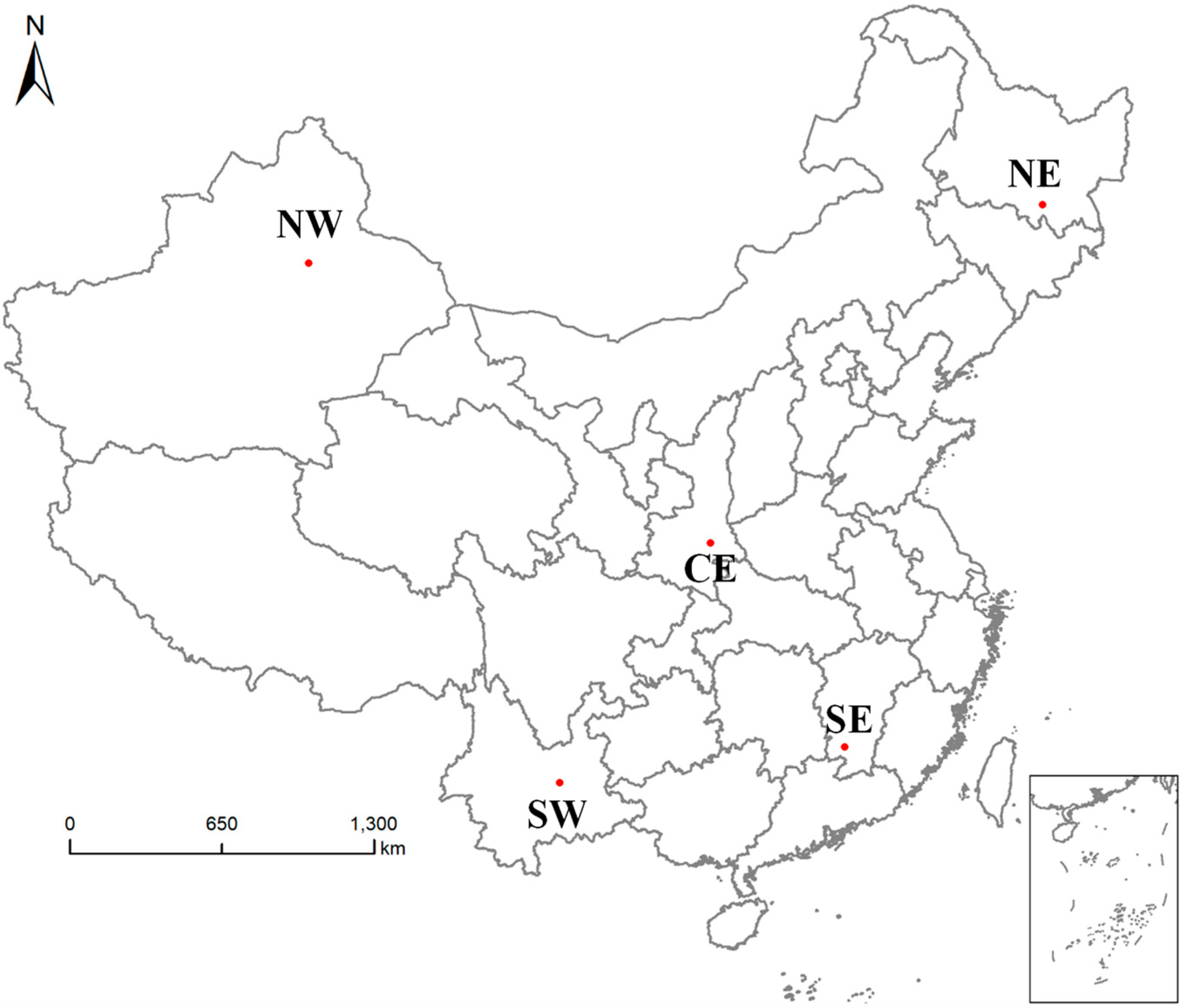
Figure 1. The five study sites in China (provincial boundaries are also shown), with the insert map showing South China Sea islands.
Remotesensing 11 02818 g001
Figure 2. Land cover maps at the five study sites for time 1 at the left column of subfigures ((a) CE, (c) NE, (e) NW, (g) SW, and (i) SE)) and time 2 at the right column of subfigures ((b) CE, (d) NE, (f) NW, (h) SW, and (j) SE)), respectively.
Remotesensing 11 02818 g002
Figure 3. Land cover change maps at the five study sites ((a) CE, (b) NE, (c) NW, (d) SW, and (e) SE).
Remotesensing 11 02818 g003
Figure 4. Flowchart of the proposed method (Fuzzy+Product).
Remotesensing 11 02818 g004
Figure 5. Probability maps of correct change categorization generated by method Fuzzy+Product based on samples of configuration 0 at different study sites: (a) CE, (b) NE, (c) NW, (d) SW, and (e) SE.
Remotesensing 11 02818 g005
Table 1. Definition of each land cover type in the study sites.
TypeDefinition
Cultivated landLand used for agriculture, horticulture, and gardens, including paddy fields, irrigated and dry farmland, vegetable and fruit garden, etc.
ForestLand covered by trees, vegetation covers over 30%, including deciduous and coniferous forests, and sparse woodland with cover 10–30%, etc.
GrasslandLand covered by natural grass with cover over 10%, etc.
Water bodiesWater bodies in land area, including river, lake, reservoir, fish pond, etc.
Artificial surfacesLand modified by human activities, including all kinds of habitation, industrial and mining area, transportation facilities, interior urban green zones and water bodies, etc.
Bare landLand with vegetation cover lower than 10%, including desert, sandy fields, Gobi, bare rocks, saline and alkaline land, etc.
Table 2. Training samples used for experiments (time 1 for year 2000, time 2 for year 2010).
ConfigurationsNumbers of Sample Pixels
CollocatedNon-Collocated
time 1time 2time 1time 2
000630630
16363567567
2126126504504
3189189441441
4252252378378
Table 3. Significant explanatory variables for single-date classification maps with samples of different configurations at the five study sites for: (a) time 1 and (b) time 2.
Study SitesConfigurations
01234
(a)
CEclass + ent21 + con9class + dom19 + het19 + ent21 + hom7class + ent21 + con9class + ent21 + con9class + ent21 + con17 + hom3
NEclass + con5class + con5class + het5 + ent19class + het5 + ent21class + het5
NWhom21 + class + ent21hom21 + class + ent21hom21 + class + ent21class + ent21class + ent21
SWclass + hom3class + hom5class + dom3class + con5 + het5 + dom15class + het3
SEclass + hom5 + dom9class + ent5 + dom17 + dom5 + dom9 + het9 + con5class + ent5 + dom19 + con7 + ent11class + ent5 + dom19 + con7 + ent11class + ent5 + het19
(b)
CEcon7 + class + dom13 + hom3 + dom3 + ent3 + het7con7 + class + dom13class + ent7 + het15 + ent21 + con15- + dom3 + ent3 + hom5 + con17 + ent11 + ent19 + het19 + het21con7 + class + het15 + ent21 + con15 + dom3 + ent3 + het19 + het21 + con19 + ent11 + het7con7 + class + dom19 + dom21 + dom3 + ent3 + hom13
NEcon7 + class + hom3 + hom5 + hom17ent3 + dom5 + classent3 + dom7 + classent3 + class + con17ent3 + class + ent15
NWclass + hom9 + con7 + dom21 + het19 + dom13 + con11 + dom9 + hom15 + het15class + hom9 + dom21 + het19 + dom13class + hom9 + dom21 + het19 + dom13class + hom9 + dom21 + het19 + dom13class + hom9 + dom21 + het19 + dom13 + het5 + hom21 + con13 + het13
SWcon15 + class + con3 + dom7 + dom9 + dom11con15 + class + het3 + dom7 + dom9 + dom11con15 + class + het3 + dom7 + het9 + het11con13 + class + het3 + dom11con13 + class + het3 + dom11 + dom7 + dom9
SEent3 + class + ent15ent3 + class + ent15ent3 + class + ent15ent3 + class + ent19 + het21 + dom21ent3 + class + ent21 + het21 + dom21
Table 4. Temporal correlation coefficients estimated for change and no-change stratum of different configurations at individual study sites in PXCOV.
Study Sites Sample Configurations
01234
CEchange0.00−0.48−0.18−0.10−0.14
no-change0.831.001.000.510.78
NEchange0.00−0.04−0.02−0.02−0.03
no-change1.001.001.001.000.70
NWchange0.00−0.21−0.10−0.11−0.06
no-change1.001.001.000.920.80
SWchange0.00−0.05−0.07−0.08−0.01
no-change1.000.790.941.000.86
SEchange0.000.060.08−0.010.00
no-change0.451.001.000.770.77
Table 5. AUC measures for the model training sample sets of different configurations at individual study sites using methods: (I) Fuzzy+Product, (II) PXCOV, (III) Fuzzy, and (IV) Product.
Study SitesMethodsConfigurations
01234
CEI0.840.840.830.840.84
II0.860.890.860.840.86
III0.770.740.760.780.76
IV0.780.780.790.800.79
NEI0.720.700.700.720.72
II0.730.710.720.720.72
III0.720.700.710.710.71
IV0.720.700.700.700.71
NWI0.750.780.780.790.79
II0.750.790.790.800.79
III0.730.760.770.780.78
IV0.750.780.790.800.79
SWI0.800.810.810.810.81
II0.810.810.810.820.81
III0.780.790.780.790.79
IV0.780.780.790.790.79
SEI0.710.710.710.710.71
II0.710.720.720.710.71
III0.700.690.700.690.70
IV0.700.700.700.690.70
Table 6. AUC differences between alternative methods for accuracy predictions based on model training sample sets of different configurations at individual study sites (*: significant at a level of 5%): (I) Fuzzy+Product, (II) PXCOV, (III) Fuzzy, and (IV) Product.
Study SitesMethods PairsConfigurations
01234
CEI versus II−0.02−0.05−0.03−0.00−0.02
I versus III0.07 *0.09 *0.07 *0.06 *0.08 *
I versus IV0.07 *0.05 *0.04 *0.04 *0.06 *
NEI versus II−0.01−0.01−0.02−0.01−0.01
I versus III0.00−0.01−0.000.01 *0.00
I versus IV0.00−0.000.010.01 *0.00
NWI versus II−0.01−0.01−0.01−0.01−0.00
I versus III0.01 *0.01 *0.01 *0.01 *0.01 *
I versus IV−0.01−0.00−0.01−0.01−0.00
SWI versus II−0.01−0.01−0.01−0.01−0.00
I versus III0.02 *0.02 *0.02 *0.02 *0.02 *
I versus IV0.02 *0.02 *0.02 *0.02 *0.02 *
SEI versus II0.00−0.01−0.01−0.00−0.00
I versus III0.01 *0.01 *0.02 *0.02 *0.01 *
I versus IV0.01 *0.01 *0.01 *0.01 *0.01 *