Study on the Intensity and Coherence Information of High-Resolution ALOS-2 SAR Images for Rapid Massive Landslide Mapping at a Pixel Level

Abstract

A rapid mapping of landslides following a disaster is important for coordinating emergency response and limiting rescue delays. A synthetic aperture radar (SAR) can provide a solution even in harsh weather and at night, due to its independence of weather and light, quick response, no contact and broad coverage. This study aimed to conduct a comprehensive exploration on the intensity and coherence information of three Advanced Land Observing Satellite-2 (ALOS-2) SAR images, for rapid massive landslide mapping in a pixel level, in order to provide a reference for future applications. Applied data were two pre-event and one post-event high-resolution ALOS-2 products. Studied area was in the east of Iburi, Hokkaido, Japan, where massive shallow landslides were triggered in the 2018 Hokkaido Eastern Iburi Earthquake. Potential parameters, including intensity difference (d), co-event correlation coefficient (r), correlation coefficient difference ($∆r$), co-event coherence ($\mathsf{\gamma }$), and coherence difference ($∆\mathsf{\gamma }$), were first selected and calculated based on a radar reflection mechanism, to facilitate rapid detection. Qualitative observation was then performed by overlapping ground truth landslides to calculated parameter images. Based on qualitative observation, an absolute value of d ($d_{abs1}$) was applied to facility analyses, and a new parameter ($d_{abs2}$) was proposed to avoid information loss in the calculation. After that, quantitative analyses of the six parameters ($d_{abs1}$, $d_{abs2}$, r, $∆r$, $\mathsf{\gamma }$ and $∆\mathsf{\gamma }$) were performed by receiver operating characteristic. $d_{abs2}$ and $∆r$ were found to be favorable parameters, which had the highest AUC values of 0.82 and 0.75, and correctly classified 69.36% and 64.57% landslide and non-landslide pixels by appropriate thresholds. Finally, a discriminant function was developed, combining three relatively favorable parameters ($d_{abs2}$, $∆r$, and $∆\mathsf{\gamma }$) with one in each type, and achieved an overall accuracy of 74.31% for landslide mapping.

1. Introduction

Landslides, defined as the movement of a mass of rock, debris, or earth down a slope [1], represent problematic and widespread geo-hazards worldwide [2], causing casualties, economic loss and property damage in mountainous areas. They can be triggered by both natural phenomenon (e.g., earthquakes and intense or prolonged rainfall) and anthropogenic activities (e.g., underground mining and reservoir construction), or a combination of them. Globally, they were said to result in about 1000 deaths and US 4 billion property damage per year [3]. Earthquake-induced landslides are considered one of the most important second hazard induced by earthquakes. Approximately 70% of all earthquake-related casualties not caused by shaking were caused by triggered landslides [4,5]. From 2004 to 2010, 47,736 causalities caused by earthquake-triggered landslides were reported [5,6,7]. Moreover, as a secondary disaster, the earthquake-induced landslides can disrupt communication, transportation, power, and even electricity service, isolating remote communities and interfering with emergency rescue. Thus, a rapid mapping of landslides following a disaster event, especially an earthquake event, is important for coordinating emergency response efforts and limiting rescue arrangement delays.

Remote sensing, especially optical sensors and synthetic aperture radar (SAR), can provide a valuable data source for rapid landslide mapping, owing to their quick response, no contact, and broad coverage. Optical sensors can provide optical images like human eyes to view the Earth, which are easy to interpret. Over the years, various optical images have been explored for landslide research through various means, either in an object level or in a pixel level. For instance, Sun et al. [8] developed an algorithm for recognizing and mapping loess landslides, based on an object-oriented approach, by combining spectral, textural, and morphometric information with auxiliary topographic parameters, in high-resolution multispectral CF-1 satellite data and a high-precision digital elevation moel (DEM). The multi-scale segmentation and merging in object-oriented analysis were executed to obtain favorable landslide candidate objects; Chen et al. [9] proposed an object-oriented landslide mapping framework, based on random forests and mathematical morphology, using ZY-3 satellite imagery. Random forest was first employed as a feature reduction tool, to identify significant features for landslide description. Mathematical morphology was then combined with the random forest to map the landslides; Bivic et al. [10] applied two image correlator software packages (MicMac and Cosi-Corr) to ortho-rectified SPOT-5 images, in order to evaluate the possibility of measuring the displacement occurred between two image acquisitions of a landslide located in a mountainous highly vegetated areas. In their study, the scale invariant feature transform method was employed to select image control points. Nevertheless, optical sensors are passive remote sensing using visible light, which rely heavily on sunlight for imaging, and cannot penetrate clouds. That may cause long time delay in acquiring favorable images, which largely hampers their application as an emergency tool for landslide mapping. In the 2015 Nepal earthquake, for instance, Burrows et al. [11] indicated that there was almost no cloud-free imagery available for landslide mapping in the first week following the disaster.

SAR data, conversely, are relatively difficult to interpret, but can be acquired at night and in any weather conditions, owing to the active characteristics of radar sensors and long wavelengths of applied microwaves. Therefore, they are deemed to be promising tools for quick response following a disaster even in harsh weather and at night. Actually, since the 1995 Kobe earthquake, SAR data have been widely investigated for building damage assessment in urban areas following a disaster e.g., [12,13,14,15,16,17], due to their advantage of weather and light independence. As active remote sensing, SAR sends electromagnetic microwaves to ground targets in a slanted way and then receives corresponding backscattering echoes. Under certain modes, it has the ability to obtain both intensity and phase information of the backscattering waves. Intensity refers to the amplitude information of the backscattering waves that can be influenced by both parameters of radar systems and characteristics of ground targets. Phase indicates the relative position of the backscattering waves within a full period, which is largely dependent on the distance between radar sensor and ground targets. The path length of an electromagnetic signal to the ground and back usually contain a number of a whole wavelength plus some fraction of a wavelength. Phase information, especially phase difference, has already been widely employed for the monitoring of slow-moving landslides through various interferometry techniques, e.g., [18,19,20,21,22,23]. Nevertheless, the feasibility of interferometry technique depends on many observation characteristics such as the spatial baseline, temporal baseline, coherence, and wavelength [24], and is restricted by many actual conditions such as the steepness and orientation of the slope as well as the amount of vegetation [25]. For instance, a favorable interferogram cannot be generated by the pre- and post-event Advanced Land Observing Satellite-2 (ALOS-2) images applied in this case owing to the low coherence between them.

For the application of SAR images in landslide mapping, especially massive landslide mapping, there have not been many investigations. Several conducted studies were only concentered on individual landslides, catchments [26,27,28], or dozens of landslides [24]. A couple of studies [11,29] focusing on large-scale landslide detection were based on the coherence or intensity information of a of series C-band Sentinel-1 SAR images. Xue et al. [26] synthesized a color image using SAR interference correlation value (red), backscattered intensity (green), and the difference between the backscattered intensities (blue), for the interpretation of the Daguanbao–Hongdongzigou giant landslide. Raspini et al. [27] exploited both amplitude (through speckle tracking) and phase (through multi-image SAR interferometry) information of SAR images, for the displacement mapping of a single large landslide in Montescaglioso, Italy. Yun et al. [28] found their damage proxy map, which was generated using the coherence difference calculated by a pre-event coherence map and a histogram-matched co-event coherence map, could roughly delineate the extent of debris from reported landslide/avalanche in Langtang valley. Konishi and Suga [24] investigated the potential of backscattering coefficient difference and intensity correlation calculated by pre- and post-event Constellation of Small Satellites for Mediterranean basin Observation (COSMO-SkyMed) images, for the detection of dozens of deep-seated landslides. Burrows et al. [11] tested three potential SAR-coherence-based landslide methods (i.e., the absolute coherence method using one pre-event and one post-event SAR images, the Advanced Rapid Imaging and Analysis (ARIA) method applying two pre-event and one post-event images [26], and the newly proposed sibling-based coherence method employing a series of SAR images) for large-scale landslide classification, in the 2015 Gorkha, Nepal earthquake, using Sentinel-1 images. Mondini [29] measured pixel-based changes between consecutive couples of sixteen Sentinel-1 SAR intensity images using Log-Ratio index, for rainfall-triggered landslide detection in Tozang area, Myanmar. Moran’s I index and semivariance were used to measure spatial autocorrelation evolution in the Log-Ratio index layers, and employed for landslide identification.

This study aimed to conduct a comprehensive exploration on the intensity and coherence information of two pre-event and one post-event L-band ALOS-2 SAR products, for rapid massive landslide mapping at a pixel level. The capability of intensity and coherence information for landslide detection would be compared to provide a reference for future applications. Both types of information are relatively easy to acquire and apply, as their feasibility does not have so many requirements for observation conditions as the interferogram. All potential parameters that can be derived relatively easily from the intensity and coherence information of the three products was selected and calculated to facilitate rapid detection. Qualitative and quantitative analyses was performed to compare the capability of these potential candidate parameters for landslide mapping so as to provide a reference. The combinational use of these information for landslide mapping was also explored.

2. Study Area and Dataset

The study area is in the east of Iburi, Hokkaido, Japan, where massive landslides were triggered in the 6.6 Mw Hokkaido Eastern Iburi Earthquake of 2018. This earthquake occurred at the epicenter of 42.686°N, 141.929°E with a depth of 35 km, at 03: 08 am local time (JST) on 6 September 2018 (UTC: 18:08 on 5 September 2018) [30,31], just one day after the powerful Typhoon Jebi passed. It induced approximately 6000 landslides over an area of around 400 km² near the towns of Atsuma, Mukawa and Abira, which caused more than 80% of the casualties in the disaster [31,32]. The number and total area of the triggered landslides were said to be the largest in Japan ever since Meiji Era [33]. The predominant bedrock and surface soil of the area is Middle to Late Miocene non-marine sediments and pyroclastic fall deposits, respectively. Surface soil layers covering low to middle mountain ranges are inter-bedded with the pumice and ash, with a total thickness of around 4–5 m in and around the epicenter area. Most triggered landslides were shallow, several meters deep-seated, moving down the pyroclastic fall deposit layer with high mobility and long run-out, and leaving the upper slip surface exposed without overlapping slide mass. The landslides are mainly spoon types and planar types with a small to medium size. Moreover, the landslide distribution demonstrated that the mostly affected terrain has an elevation of 100–250 m, and a slope gradient of 15–35° [32,34].

The applied dataset are three ALOS-2 single look complex (SLC) products acquired in the affected areas before and after the disaster on 9 August, 23 August, and 6 September. All three images covered the same region with an area of 55 km × 70 km (Figure 1a) captured from the left looking ascending track with an off-nadir angle of 37.8°. SLC products means that the images were represented by complex I and Q channels to preserve magnitude and phase information, from which intensity and coherence can be derived. The acquisition mode of these images was stripmap ultra-fine mode single polarization (UBS), with a polarization mode of HH. A summary of the data information was listed in

Table 1. Information of the applied ALOS-2/PALSAR-2 data.

Date (UTC) (yyyy/mm/dd)	Format	Level	Mode	Polarization	Sample Spacing (Range × Azimuth)	Orbit Direction	Off-nadir Angle
2018/08/09	CEOS	L1.1 (SLC)	UBS	HH	1.43m × 1.95m	Left Looking/Ascending	37.8°
2018/08/23	CEOS	L1.1 (SLC)	UBS	HH	1.43m × 1.95m	Left Looking/Ascending	37.8°
2018/09/06 (13:37)	CEOS	L1.1 (SLC)	UBS	HH	1.43m × 1.95m	Left Looking/Ascending	37.8°

ALOS-2: Advanced Land Observing Satellite-2; PALSAR-2: Phased Array type L-band Synthetic Aperture Radar-2; CEOS: Committee on Earth Observation Satellites; SLC: single look complex; UBS: ultra-fine mode single polarization; HH: horizontal transmit/horizontal receive.

. A rectangular region in the landslide area covered by the three SAR images was selected as the study area (Figure 1a).

The Geospatial Information Authority of Japan (GSI) released a first-hand landslide database several days after the earthquake. Nevertheless, most of the released landslides consist of several or dozens of landslides. Based on high-resolution aerial images and ridge lines, valley lines, hillshade, and slop aspect generated by a 10 m resolution DEM, Zhang et al. [34] conducted a manual segmentation and combination of this released landslide database regarding the unreasonable landslide units, and created a detailed landslide inventory map. In this study, the detailed landslide inventory map created by Zhang et al. [34] was used as the ground truth landslide data for result comparison and evaluation. The distribution of the ground truth landslides in the study area was shown in Figure 1b.

3. Methodology

3.1. Principle and Parameter Calculation

The applied ALOS-2 SLC products obtained both intensity and phase information of microwave backscattering echoes from ground targets. Intensity indicates the amplitude information of backscattering microwaves received by the SAR sensor after emitting microwaves to ground targets. It is influenced by not only radar system parameters (e.g., frequency, polarization, and incidence angles) but also ground target characteristics (e.g., roughness and material dielectric characteristics). Therefore, intensity changes in SAR images over a period of time can indicate the ground target changes during this time. As landslides usually cause land surface changes such as de-vegetation and slope smoothing, SAR image intensity changes are deemed to have the potential for landslide identification. Intensity difference and co-event correlation coefficient calculated by pre- and post-event SAR images can be used to quantify SAR image intensity changes caused by a disaster event, and hence are selected as candidate parameters for landslide mapping in this case.

Intensity difference, d, can be easily calculated by Equation (1). Regions with higher absolute values of d experienced larger ground changes, whereas regions with lower absolute values of d experienced smaller changes.

$$d=\frac{{{\displaystyle \sum }}_{i=1}^N\left(I{b}_i-I{a}_i\right)}{N}$$

(1)

where N is the total number of pixels within a certain window, and $I{a}_i$ and $I{b}_i$ are intensity values of pixel i in the two SAR images (hereafter).

Correlation coefficient, r, can be calculated according to Equation (2). Its values range from −1 to 1, with lower values indicating larger ground changes, and a 1 value representing no ground changes.

$$r=\frac{N{{\displaystyle \sum }}_{i=1}^{N}I{a}_{i}I{b}_i-{{\displaystyle \sum }}_{i=1}^{N}I{a}_i{{\displaystyle \sum }}_{i=1}^{N}I{b}_i}{\sqrt{\left(N{{\displaystyle \sum }}_{i=1}^{N}I{a}_i^2-{\left({{\displaystyle \sum }}_{i=1}^{N}I{a}_i\right)}^2\right)·\left(N{{\displaystyle \sum }}_{i=1}^{N}I{b}_i^2-{\left({{\displaystyle \sum }}_{i=1}^{N}I{b}_i\right)}^2\right)}}$$

(2)

Moreover, to differentiate areas where the correlation coefficient value is always low and where it has decreased, the difference of pre-event and co-event correlation coefficient, $∆r$, was also calculated (Equation (3)) and taken into account. This parameter has shown favorable performance for building damage detection in un-urbanized areas shown favorable performance for building damage detection in un-urbanized areas [35].

$$∆r=r_{co}-r_{pre}$$

(3)

where r_co is the co-event correlation coefficient calculated by one pre-event and one post-event SAR images, and r_pre is the pre-event correlation coefficient calculated by two pre-event SAR images.

Phase is a property of periodic phenomenon, referring to the relative value of received backscattering waves within the span of a full period. It is very sensitive to the distance between the satellite sensor and ground target, and hence also has the ability to measure ground target changes. Phase difference has already been applied through SAR interferometry techniques to measure earth’s surface changes, such as the deformation caused by landslides, volcanoes, glaciers or anthropogenic activities [36]. Nevertheless, the feasibility of the interferometry technique depends on many observation characteristics (e.g., spatial baseline, temporal baseline, coherence, and wavelength) [24], and is restricted by many actual conditions when applied for landslide detection and monitoring (e.g., the steepness and orientation of the slope and the amount of vegetation) [25]. In this case, a favorable interferogram cannot be generated by the pre- and post-event SAR images due to the low coherence between them.

Coherence, $\mathsf{\gamma }$, means the cross-correlation of phase information in two images (Equation (4)), which is often used to prejudge whether a good interferogram can be generated. Its values range from 0 to 1, and it can also be applied to measure ground changes, with a lower value indicating larger ground changes. Therefore, in this case, the co-event coherence calculated by one pre-event and one post-event SAR image was also selected as a candidate parameter for landslide mapping in this case. Moreover, similar to the correlation coefficient, to distinguish areas where the coherence value is always low and where it has reduced, the difference of pre-event and co-event coherence, $∆\mathsf{\gamma }$, was also calculated (Equation (5)) and explored.

$$\mathsf{\gamma }=\frac{E\langle c_1{c}_2^{*}\rangle }{E\langle c_1{c}_1^{*}\rangle E\langle c_2{c}_2^{*}\rangle }$$

(4)

where c₁ and c₂ are corresponding complex pixel values in images of two acquisition dates, c^* means the complex conjugate of c, and E means the expected value.

$$∆\mathsf{\gamma }={\gamma }_{co}-{\gamma }_{pre}$$

(5)

where ${\gamma }_{co}$ is the co-event coherence calculated by one pre-event and one post-event SAR images, and ${\gamma }_{pre}$ is the pre-event coherence calculated by two pre-event SAR images.

To sum up, all of the parameters mentioned above, including intensity difference d, co-event correlation coefficient r, correlation coefficient difference $∆r$, co-event coherence $\mathsf{\gamma }$, and coherence difference $∆\mathsf{\gamma }$, have certain potential for landslide mapping, and were selected as candidate parameters in this case. In order to obtain images of these parameters, the Sentinel Application Platform (SNAP) 6.0 of the European Space Agency (ESA) and ArcGIS 10.5 software of the Environmental Systems Research Institute (ESRI) were applied to process the three original SAR SLC products. SNAP 6.0 was primarily applied to extract basic intensity and coherence information from the original complex images [37]. ArcGIS 10.5 was mainly employed for the final calculation of these potential parameters.

3.2. Qualitative and Quantitative Analyses of Potential Parameters

After obtaining images of these potential parameters, qualitative and quantitative analyses were carried out to investigate the performance of these parameters for landslide detection. Qualitative analyses were carried out by overlapping the landslide ground truth data [34] upon the calculated parameter images. Observing the parameter characteristics in actual landslide and non-landslide areas can intuitively show their capabilities for landslide mapping.

Quantitative analyses of the parameters were executed by receiver operating characteristic (ROC) curves. ROC curves are graphical plots generated by true positive rate (TPR) values against false positive rate (FPR) values, and can be used to illustrate the diagnostic ability of binary classifiers [38,39,40]. In a binary classification problem, under a certain threshold, there is a confusion matrix composed of four elements: true positive (TP), true negative (TN), false positive (FP), and false negative (FN), according to actual and predicted classification results (

Table 2. Confusion matrix for a binary classification problem.

	Predicted	Positive	Negative
Actual
Positive		True Positive (TP)	False Negative (FP)
Negative		False Positive (FP)	True Negative (TN)

). Based on these four elements in the confusion matrix, TPR and FPR can be calculated easily by Equations (6) and (7). Moving the classification threshold from lower values to higher values, a series of TPR and FPR can be obtained, by which a ROC curve is able to be generated. On the one hand, the ROC curve can be applied to measure and compare the performance of binary classifiers through calculating the area under the curve (AUC). Values of AUC range from 0.5 to 1, with a larger value representing a model with higher performance [41]. On the other hand, for a specific binary model, the ROC curve can be employed to find the optimal classification threshold by seeking the point with highest Youden index [42] in the top left.

TPR = TP/(TP + FN)

(6)

where TP is the true positive, and FN is the false negative.

FPR = FP/(FP + TN)

(7)

where FP is the false positive, and TN is the true negative.

Parameter calculation window sizes influence characteristics of calculated parameter images (e.g., ground target boundary), and will also affect the performance of the parameters as landslide classifiers. To understand the influence of window sizes as well as to find the optimal window size, the equal step and hunt&fill scaling method [43,44,45] in incremental dynamic analysis were referred to in order to save computational efforts. First, calculation window sizes of 5 × 5, 15 × 15, 25 × 25, 35 × 35, 45 × 45, 55 × 55, 65 × 65, 75 × 75, and 85 × 85 were applied to understand the overall trend of window size impacts, as the pixel size of applied SAR images is around 3 square meters, and the landslide sizes in the study areas vary from hundreds to tens of thousands square meters. Then, if big differences exist between the results of two adjacent calculation window sizes, interpolation will be carried out to fill the gap and hunt for the specific optimal window size.

4. Results

4.1. Parameter Qualitative Observations

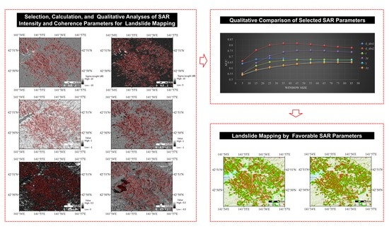
The calculated parameter images overlapped by ground truth landslides were shown in Figure 2. As can be seen from this figure, more or less, all potential parameters showed some different characteristics in landslide and non-landslide areas.

The intensity difference image (Figure 2a) displays some obvious higher-value and lower-value pixels in landslide areas. That means both increase and decrease of intensity have been caused by the earthquake-induced landslides. On the one hand, triggered landslides wiped away many elements on the hillsides (e.g., trees and big stones), smoothing the slopes, which reduced the backscattering from the slope to the radar sensor, and hence caused the intensity decrease. On the other hand, the alluviums washed away by landslides deposited in some foot regions of the slope, increasing the backscattering from these areas to the radar sensor, therefore inducing the intensity increase.

As both intensity increase and decrease occurred in landslide areas, the absolute value of the intensity difference, d_abs1, was calculated (Equation (8)) and would be applied to facilitate further analysis for landslide pixel identification. In the image of this parameter, landslide areas will only display higher-value pixels (Figure 2b). Furthermore, information loss may occur when calculating d and $d_{abs1}$ according to Equation (1), as the increased and decreased intensity pixel values within the calculation window could be averaged and neutralized. Therefore, a new intensity difference absolute value, $d_{abs2}$, was created (Equation (9)) to avoid information loss in intensity difference calculation, and would also be explored as a landslide classifier.

$$d_{abs1}=\left|d\right|$$

(8)

where d is the intensity difference calculated by Equation (1).

$$d_{abs2}=\frac{{{\displaystyle \sum }}_{i=1}^N\left|I{b}_i-I{a}_i\right|}{N}$$

(9)

In both co-event correlation coefficient (Figure 2c) and correlation coefficient difference (Figure 2d) images, landslide areas display some lower-value pixels, indicating larger ground changes compared with non-landslide areas. Due to larger backscattering changes in the post-event SAR image caused by landslide-induced ground changes, the co-event correlation coefficient in the landslide areas became relatively smaller, leading to these lower-value pixels. Besides, by subtracting a pre-event correlation coefficient, some areas where pixel values were always low seem to be excluded as expected. For instance, the water area at the top left of the study region (blue polygon in Figure 3), which showed relatively lower pixel values in the correlation coefficient image (Figure 2c), did not show clear lower pixel values in the correlation coefficient difference image (Figure 2d) anymore.

The co-event coherence (Figure 2e) and coherence difference (Figure 2f) images also display some lower-value pixels in some landslide areas, owing to the decorrelation caused by landslide-involved ground changes. Nevertheless, the difference between landslide and non-landslide areas in these two images seems to be not as clear as that in other images. This may be due to the fact that most study areas were covered by trees where the coherence is originally very low even no landslides occurred. A clear lower-value region can be seen in the darker area of the coherence difference image (Figure 2f). This area was initially grassland (green polygon in Figure 3), which had higher pre-event coherence values compared with areas covered by trees. Therefore, when pre-event coherence was subtracted from the co-event coherence, a lower-value area region appears.

4.2. Parameter Quantitative Analyses

ROC analyses of the six parameters mentioned above ($d_{abs1}$, $d_{abs2}$, r, $∆r$, $\mathsf{\gamma }$, and $∆\mathsf{\gamma }$) calculated under different window sizes were carried out one by one. Obtained AUC values were listed in

Table 3. Area under the curve (AUC) values of the six parameters calculated under different window sizes.

	5×5	15×15	25×25	35×35	45×45	55×55	65×65	75×75	85×85
$d_{abs1}$	0.6385	0.6763	0.6856	0.6833	0.6745	0.6639	0.6551	0.6504	0.6483
$d_{abs2}$	0.6601	0.7552	0.7998	0.8153	0.8148	0.8063	0.7954	0.7851	0.7768
r	0.5537	0.6203	0.6525	0.6672	0.6729	0.6745	0.6742	0.6739	0.6741
$∆r$	0.5519	0.6437	0.7050	0.7388	0.7523	0.7540	0.7503	0.7447	0.7392
$\mathsf{\gamma }$	0.5406	0.5794	0.6042	0.6217	0.6352	0.6482	0.6580	0.6648	0.6690
$∆\mathsf{\gamma }$	0.5436	0.5842	0.6070	0.6242	0.6356	0.6435	0.6482	0.6511	0.6521

and then plotted in Figure 4 for easy visual observation. As can be seen from the table and the figure, the newly proposed parameter $d_{abs2}$ shows the largest AUC values among all parameters, indicating its best performance as landslide classifiers in this case. The correlation coefficient difference $∆r$ also shows good performance, whose AUC values are higher than the other four parameters when the calculation window size is larger than 25. Besides, the largest AUC values of $d_{abs2}$ and $∆r$ are around 0.82 and 0.75 respectively, demonstrating their favorable performance in classifying landslide and non-landslide pixels.

Moreover, in general, the intensity-related parameters ($d_{abs1}$, $d_{abs2}$, r, and $∆r$) have better performance than the coherence-related parameters ($\mathsf{\gamma }$ and $∆\mathsf{\gamma }$). This is considered to be associated with the sensitivity of these two kinds of information to ground changes. The more stable the parameter to minor ground variations, the less interference caused by other small ground changes, and hence the higher the parameter performance (i.e., larger AUC values in this case). Coherence information is more sensitive to minor changes, and usually shows low values in forests even if no disaster occurred. The study area was mainly covered by trees. Therefore, overall, the coherence-related parameters show poorer performance in this case.

In addition, between the two intensity difference parameters ($d_{abs1}$ and $d_{abs2}$), $d_{abs2}$ shows much better performance than $d_{abs1}$, demonstrating the advantage of Equation (7), which tried to avoid information loss in calculation. In addition, as the window size increases, the gap between the AUC values of $d_{abs1}$ and $d_{abs2}$ is growing increasingly larger. This also proves that information loss occurred in the calculation of $d_{abs1}$, which was caused by the average of increased and decreased intensity pixel values within the calculation window. As for the two correlation coefficient parameters (r and $∆r$), $∆r$ shows much better performance than r, as some pixels whose values were always low were excluded by subtracting one pre-event correlation coefficient image. However, this approach dose not achieve the same good effect on coherence parameters, as most of the study area was covered by trees that along can cause large coherence decorrelation. The classification performance of $∆\mathsf{\gamma }$ is as unsatisfactory as that of γ.

As for the influence of calculation window sizes, the general trend for the intensity-related parameters is that, as the window size increases, the classification accuracy first increases and then tends to stabilize or even decrease. Favorable window sizes are around 25 to 55, with the optimal being 25, 35, 55, and 55 for $d_{abs1}$, $d_{abs2}$, r, and $∆r$, respectively. Compared with other parameters, $d_{abs1}$ achieves the optimal performance in a smaller window size, as the bigger the window size, the more increased and decreased pixels will be averaged. For the coherence-related parameters, within the calculation window sizes that have been applied, the parameter performance is becoming better and better with the increase of the calculation window size. Nevertheless, the improvement is very slight.

Furthermore, as can be seen from Table 3, there is no big difference between the AUC values of parameters calculated under two adjacent optimal window sizes. Therefore, interpolation between the calculation window sizes was not carried out. The highest AUC values for the six parameters, i.e., $d_{abs1}$, $d_{abs2}$, r, $∆r$, $\mathsf{\gamma }$, and $∆\mathsf{\gamma }$, are around 0.69, 0.82, 0.67, 0.75, 0.67, and 0.65, respectively. That means, individually, $d_{abs1}$, r, $\mathsf{\gamma }$, and $∆\mathsf{\gamma }$ are not very appropriate as binary classifiers for distinguishing landslide and non-landslide pixels in this case, while $d_{abs2}$ and $∆r$ have favorable performances. What should be noted is that this conclusion is obtained based on only this specific case: mapping of massive shallow landslides with a small to medium size in slopes covered by trees, using high-resolution L-band ALOS-2 products. For images of other bands or other resolution conditions, or for landslides in bare slopes or of deep-seated or large-sized types, there may be some differences. For instance, the coherence parameters may have better performances for landslide mapping in bare slopes due to there being no vegetation interference.

4.3. Landslide Mapping by Receiver Operating Characteristic (ROC) Optimal Thresholds of the Favorable Parameters

In order to specifically understand the performances of the two favorable parameters ($d_{abs2}$ and $∆r$) found in quantitative analyses, detailed analyses were carried out. ROC curves of the two parameters calculated under the optimal window sizes were shown in Figure 5. Optimum thresholds were then determined by seeking the point with highest Youden index at the top left of the curves. Corresponding threshold values for $d_{abs2}$ and $∆r$ were 2.08 and −0.11, respectively. Classification results under the optimal thresholds were shown in Figure 6 to compare with the ground truth landslides. A summary of the classification accuracy was listed in

Table 4. Landslide mapping accuracy of $d_{abs2}$ and $∆r$ calculated under the optimum window sizes.

Parameter	Accuracy	Recall	Precision	F1 score
$d_{abs2}$	69.36%	87.76%	47.04 %	61.25%
$∆r$	64.57%	81.68 %	42.59%	55.99%

, including accuracy, recall, precision, and F1 score, to provide a quantitative understanding. Accuracy is an intuitive performance measure, indicating the ratio of correctly predicted observations to total observations (Equation (10)). Recall is defined as the correctly predicted positive observations divided by all observations in actual class (Equation (11)). Precision is defined as the correctly predicted positive pixels divided by the total predicted positive pixels (Equation (12)). F1 score is a weighted average of recall and precision [46], calculated based on Equation (13) to achieve a balance between the recall and precision measure.

Accuracy = (TP + TN)/(TP + TN + FP + FN)

(10)

Recall = TP/(TP + FN)

(11)

Precision = TP/(TP + FP)

(12)

F1 score = 2*(Recall*Precision)/(Recall + Precision)

(13)

where TP, TN, FP, and FN are the true positive, true negative, false positive, and false negative, respectively.

The shape of ROC curves in Figure 5 can give an intuitive impression of the parameter performance as binary landslide classifiers. As the x and y axis represent TPR and FPR respectively, the closer the curve to the y axis, the better the parameter performance.

The accuracy and recall values in Table 4 can provide a quantitative understanding of the parameters capabilities for landslide and non-landslide pixel classification. When using $d_{abs2}$ as a landslide classifier, 69.36% landslide and non-landslide pixels can be correctly classified, and 87.76% landslide pixels can be correctly identified. When using $∆r$ as a landslide classifier, 64.57% landslide and non-landslide pixels can be correctly classified, and 81.68% landslide pixels can be correctly identified. Since the key point of landslide mapping is to identify all landslide areas correctly, the higher recall values indicate that the two parameters have certain values for landslide mapping.

The low precision values of the classification results (Table 4) demonstrate that many non-landslide pixels were classified as landslide pixels. This can been seen more clearly from Figure 6, which shows that many non-landslide areas around the ground truth landslides were classified as landslides by the two parameters. To some extent, this phenomenon is due to the principal of the two SAR intensity parameters. In the ground truth landslides, the landslide boundaries were generally consistent with visible ground changes, such as de-vegetation, as shown in Figure 3. Nevertheless, surrounding areas of the landslides where there seems to be no clear visible changes may also experience implicated changes, for instance, vegetation tilt caused by the erosion or lashing of surrounding soils. These implicated changes may cause the same level SAR backscattering changes as landslides, making these areas detected as landslides by the parameters. F1 score, which balanced the recall and precision measures, has a value of 61.25% for $d_{abs2}$ and a value of 55.99% for $∆r$, indicating a relatively better performance of $d_{abs2}$ compared with $∆r$ on the whole.

4.4. Landslide Mapping by Jointly Applying Three Types of Parameters through Linear Discriminant Analysis

As the sensitivities of the three types of parameters (i.e., intensity difference, correlation coefficient, and coherence) to ground changes are different, a combinational application of them may provide complementary information to each other, and improve the landslide mapping accuracy. To explore the combinational use of the three types of parameters, linear discriminant analysis [47] was carried out using three relatively favorable parameters with one in each type. Linear discriminant analysis is a mathematical process using various data items and applying functions, to separately analyze multiple classes of objects or items. It has been applied for SAR-based building damage assessments since the 1995 Kobe Earthquake, and has shown favorable performances, e.g., [12,48]. $d_{abs2}$, $∆r$, and $∆\mathsf{\gamma }$ were applied as the intensity difference, correlation coefficient, and coherence parameters, respectively, as they have shown favorable performances in parameter qualitative and quantitative analyses, and/or are able to distinguish areas where parameter values were always low and have decreased.

A discriminant function combining $d_{abs2}$, $∆r$, and $∆\mathsf{\gamma }$ was obtained from the linear discriminant analysis, and is shown in Equation (14). Landslides mapped by this discriminant function are shown in Figure 7, to provide an intuitive observation. Pixels with positive discriminant scores (z values) were assigned as landslides, whereas pixels with negative discriminant scores were assigned as non-landslides. The accuracy, recall, and precision values of the mapping results are 74.31%, 70.13%, and 52.58%, respectively. Compared with the landslides mapped by the ROC thresholds of $d_{abs2}$ and $∆r$, the accuracy and precision values are higher, and the recall value is lower. Misclassifications owing to the fact that surrounding non-landslide pixels were classified as landslide pixels seem to be reduced, even though some still exist. Some misclassified landslide pixels in the water area of Figure 6 seems to be eliminated by this method (Figure 7). What should be noted is that this discriminant function was obtained based on only this case study. For the application to other SAR images and other ground conditions, a further check is still needed, as the parameter coefficients in the function may vary with the conditions of SAR images and actual sites.

$$z=1.069d_{abs2}-1.822∆r-2.986∆\mathsf{\gamma }-3.406$$

(14)

where z is the discriminant score.

5. Discussion

In this work, a relatively comprehensive study was conducted concerning the application of intensity and coherence information in two pre-event and one post-event L-band ALOS-2 SAR products for rapid massive landslide mapping at a pixel level. Qualitative observations, quantitative analyses, and a combinational application of the potential parameters were carried out, to obtain some results and conclusions for future reference. What should be noted is that these results and conclusions were obtained based on only this one specific case: mapping of massive shallow landslides with a small to medium size in slopes covered by trees, using high-resolution L-band ALOS-2 products. For other types of landslides or other SAR images, there may be some differences, and further verifications are still needed. For instance, the coherence difference may be a good parameter for identifying landslides in slopes covered by grass (as shown in the darker area of Figure 2f). The coefficients of different parameters in the discriminant function shall vary with the landslide situations and SAR image conditions. Nevertheless, the two favorable parameters ($d_{abs2}$ and $∆r$) shall also have favorable performances for the detection of deep-seated and large-sized landslides, as ground changes induced by these types of landslides are more conspicuous. The combinational use of the three types of parameters shall lead to more obvious accuracy improvement for areas with landslides of more types or more sizes, owing to the different sensitivities of different parameters to ground changes.

Moreover, in this study, the linear discriminant analysis was applied to jointly use several different parameters, as it is relatively simple, and has shown favorable performances for SAR-based building damage assessment. Other machine learning classifiers, such as the decision tree, random forest, and support vector machine, also have good capabilities for classification problems based on a series of variables, and can be explored to jointly use the intensity and coherence information for landslide mapping. Yet, no matter which kind of classification method is applied, the trained models and parameters (e.g., coefficients of parameters in the discriminant function) shall vary with the conditions of landslides and SAR images. For an emergency application in a specific event, if such trained models are not available, an intuitive observation of the favorable parameters would be a good way, as these parameters can be calculated very easily, and have shown favorable performances even in the qualitative analyses. Furthermore, to make full use of different parameters’ advantages, the intuitive observation can also be conducted by compositing several calculated parameter images into a color image (e.g., red: intensity difference, green: correlation coefficient difference, blue: coherence difference).

In addition, it seems that a reasonable inference can be obtained concerning the parameter calculation window sizes: the more sensitive the parameter to minor ground changes, the bigger window sizes are needed to blur parameter changes caused by these minor changes in order to reduce their interference, and therefore the bigger the optimal window size. In this case, the sensitivity of these three kinds of parameters to other minor ground changes was: coherence parameters > correlation coefficient parameters > intensity difference parameters, and the optimal calculation window size for them was also: coherence parameters > correlation coefficient parameters > intensity difference parameters. Besides, the favorable window sizes for the intensity-related parameters seem to be associated with image pixel sizes and landslide area distribution. In this case, the favorable window sizes for the intensity-related parameters were about 25 to 55. The size of each pixel is approximately 3 m². The landslide areas in the study region range from 100 m² to 50,000 m², with an average value of approximately 7000 m² (between the window size of 45 and 55). Landslides with an area of less than 2000 m² (around the window size of 25) account for around 25% of the total number of landslides, and landslides with an area of less than 9000 m² (around the window size of 55) account for around 75% of the total number of landslides. Further verification of this phenomenon is still needed, yet it seems to be rational, as the performances of parameters increase first and then decrease with the increasing of calculation window sizes. Therefore, in a specific case, if possible, it is suggested to consider both the distribution of landslide areas (or at least the rough scale of most landslides) and image pixel sizes when selecting an appropriate window size for parameter calculation.

Furthermore, this study applied only SAR intensity and coherence information for rapid mapping of massive landslides. Nevertheless, when available, the polarimetry information of SAR data should also have favorable performances for landslide detection, as the changes of different scattering mechanisms (e.g., surface scattering, double-bounce scattering, and volume scattering) can clearly understood by decomposing the polarimetry data using model-based and/or eigenvalue-eigenvector-based decompositions. The fusion of other information, such as DEM, pre-event optical images, geology information, and landslide triggering factors, should also be able to improve the landslide detection accuracy, and improve the performance of some unfavorable parameters. For instance, as coherence changes are very sensitive to minor ground variations, small ground changes unrelated to landslides, such as the area change of river band caused by flood, also influence the performance of coherence information as landslide classifiers. If ancillary information, such as DEM, optical images, and land-use maps can be obtained and applied to eliminate irrelevant areas (e.g., flats and waters) first, the landslides mapped by coherence will be much more accurate.

6. Conclusions

This study provided a comprehensive exploration on the intensity and coherence information of three ALOS-2 SAR images for rapid mapping of massive densely distributed shallow landslides. Two pre-event and one post-event high-resolution ALOS-2 SLC products were processed and applied. Four intensity-related ($d_{abs1}$, $d_{abs2}$, r, and $∆r$ ) and two coherence-related ($\mathsf{\gamma }$ and $∆\mathsf{\gamma }$) potential parameters that can be derived from the three products relatively easily were selected and calculated to facilitate rapid detection, including a new parameter ($d_{abs2}$) proposed to avoid information loss in the calculation. Visual observation and ROC analyses were performed to analyze and compare these parameters for landslide mapping qualitatively and quantitatively, in order to give a reference for future applications. The new intensity difference parameter $d_{abs2}$ and correlation coefficient difference $∆r$ showed favorable performance, and were further explored to classify landslide and non-landslide pixels by suitable thresholds. A discriminant function was developed jointly applying these two types of information, by combining three relatively favorable parameters ($d_{abs2}$, $∆r$, and $∆\mathsf{\gamma }$) with one in each type, using linear discriminant analysis, for landslide mapping. Several conclusions obtained from this study are summarized as follows.

Qualitatively, intensity difference showed clear lower-value and higher-value pixels in landslide areas, as triggered landslides smoothed hillsides, causing backscattering decrease, and roughened foothill areas that induced backscattering increase. Co-event correlation coefficient and correlation coefficient difference displayed lower-value pixels in landslide regions due to larger ground changes induced by landslides. Co-event coherence and coherence difference also showed some lower-value pixels in landslide areas owing to the decorrelation caused by landslide-involved ground changes.

Quantitatively, intensity-related parameters showed better performance than coherence-related parameters as they are more stable to other minor ground changes. The new intensity difference parameter $d_{abs2}$ and correlation coefficient difference $∆r$ showed favorable performance as landslide and non-landslide pixel classifiers, and are recommended for future applications. In particular, $d_{abs2}$ can achieve an AUC value of around 0.82 under the optimal window size, and can be derived easily from only one pre-event and one post-event SAR intensity images. Nevertheless, the largest AUC values of other four parameters ($d_{abs1}$, r, $\mathsf{\gamma }$, and $∆\mathsf{\gamma }$) were around 0.65–0.69, indicating that, individually, they are not very appropriate binary classifiers for distinguishing landslide and non-landslide pixels in this case. Furthermore, between the two intensity difference parameters ($d_{abs1}$ and $d_{abs2}$), $d_{abs2}$ showed better performance than $d_{abs1}$, demonstrating the advantage of considering avoiding information loss in parameter calculation. Between the two correlation coefficient parameters (r and $∆r$), $∆r$ showed improved performance, as pixels whose values were always low can be excluded by subtracting one pre-event correlation coefficient image.

In addition, the landslide mapping results demonstrated that, individually, the two favorable parameters ($d_{abs2}$ and $∆r$) correctly classified around 64–69% landslide and non-landslide pixels by simple ROC thresholds. The combinational application of the intensity difference, correlation coefficient, and coherence parameters ($d_{abs2}$, $∆r$, and $∆\mathsf{\gamma }$) through linear discriminant analysis achieved an overall accuracy of around 74%. Misclassification is mainly due to the fact that some non-landslide pixels around the ground truth landslides were classified as landslide pixels, as landslide surroundings where there seems to be no clear visible changes may have experienced implicated changes (e.g., tree tilt caused by alluvium erosion or lashing).

Last but not least, we acknowledge that some conclusions have limitations, as they were obtained based on only this case study: mapping of massive shallow landslides with a small to medium size in slopes covered by trees, using high-resolution L-band ALOS-2 products. For instance, the poor performance parameters in this case may have better performance for landslide mapping on bare slopes, owing to the absence of vegetation interference. Further studies are still needed for other types of SAR data and other types of landslides. Moreover, this study aimed to provide a rapid way for massive landslide mapping applying only SAR intensity or coherence information. Nevertheless, when available, the fusion of other information, such as DEM, pre-event optical images, geology information, or landslide triggering factors, should be able to improve the landslide detection accuracy.