Abstract
Polarimetric synthetic aperture radar (PolSAR) remote sensing has been widely used for forest mapping and monitoring. PolSAR data has the capability to provide scattering information that is contributed by different scatterers within a single SAR resolution cell. A methodology for a PolSAR-based extended water cloud model (EWCM) has been proposed and evaluated in this study. Fully polarimetric phased array type L-band synthetic aperture radar (PALSAR) data of advanced land observing satellite (ALOS) was used in this study for forest aboveground biomass (AGB) retrieval of Dudhwa National Park, India. The shift in the polarization orientation angle (POA) is a major problem that affects the PolSAR-based scattering information. The two sources of POA shift are Faraday rotation angle (FRA) and structural properties of the scatterer. Analysis was carried out to explore the effect of FRA in the SAR data. Deorientation of PolSAR data was implemented to minimize any ambiguity in the scattering retrieval of model-based decomposition. After POA compensation of the coherency matrix, a decrease in the power of volume scattering elements was observed for the forest patches. This study proposed a framework to extend the water cloud model for AGB retrieval. The proposed PolSAR-based EWCM showed less dependency on field data for model parameters retrieval. The PolSAR-based scattering was used as input model parameters to derive AGB for the forest area. Regression between PolSAR-decomposition-based volume scattering and AGB was performed. Without deorientation of the PolSAR coherency matrix, EWCM showed a modeled AGB of 92.90 t ha−1, and a 0.36 R2 was recorded through linear regression between the field-measured AGB and the modeled output. After deorientation of the PolSAR data, an increased R2 (0.78) with lower RMSE (59.77 t ha−1) was obtained from EWCM. The study proves the potential of a PolSAR-based semiempirical model for forest AGB retrieval. This study strongly recommends the POA compensation of the coherency matrix for PolSAR-scattering-based semiempirical modeling for forest AGB retrieval.
1. Introduction
Spaceborne polarimetric synthetic aperture radar (SAR) remote sensing has been extensively used for structural and bio-geophysical parameters retrieval of manmade and natural features [1]. Several researchers have explored the capabilities of SAR systems for ecological applications [2,3]. Forest aboveground biomass is an important ecological parameter that directly indicates the plant biomass energy [4,5]. The sensitivity of SAR backscatter has been analyzed by previous researchers to develop modeling approaches for forest aboveground biomass (AGB) estimation [6,7,8,9]. Most of the studies carried out to develop modeling approaches for forest AGB estimation have used single or dual-polarimetric SAR data [3,10,11]. The main limitation of SAR-data-based modeling for forest AGB is the retrieval of scattering components of vegetation and ground in a SAR resolution cell. Model-based structural and biophysical parameter retrieval of a forest area requires information about different types of scatterers within a single pixel or resolution cell of SAR data acquired over the study area. A single resolution cell of a SAR image may contain different types of scatterers and their contribution to scattering is required to develop any modelling approach. Previous studies had used single- or dual-polarized channels of SAR data to mathematically derive the amount of scattering contributed by different features in the total backscatter value of the particular resolution cell [12,13]. The procedure to calculate the approximate values of scattering of different features was very complex.
Acquisition of fully polarimetric SAR data in all of the four possible polarization combinations of transmitted and received electromagnetic signals provides the potential for SAR data to retrieve information of different features within a single SAR resolution cell [14,15]. Retrieval of scattering from SAR data depends on structural and dielectric properties of the object and the selection of a particular wavelength, angle of incidence, and polarization of the sensor. PolSAR-decomposition-based modeling approaches have been developed in the last few years to retrieve reliable scattering from a PolSAR single resolution cell. The initial decomposition models were developed with the modeling of a lexicographic feature vector-based PolSAR covariance matrix. It was observed that the scattering retrieval from PolSAR decomposition suffers from the ambiguities in the scattering mechanism, which occurs due to the shift in polarization orientation angle (POA) of the polarization ellipse of the electromagnetic wave [16,17,18]. The shift in POA occurs due to the rotation of the polarization basis of the scattering matrix of quad-pol SAR data [19]. The POA shift resulted as an overestimation of volume scattering and an underestimation of double-bounce scattering during the model-based decomposition of PolSAR data. The shift in polarization orientation angle (POA) of the polarization ellipse of the electromagnetic wave occurs or was introduced due to the Faraday rotation and the structural properties of the ground targets. The Faraday rotation angle (FRA) is introduced in the polarization ellipse due to the propagation of electromagnetic waves through the magnetic field of the ionosphere [20]. Generally, the PolSAR data, which is provided to the users, are free from the POA shift caused by the Faraday rotation. The structural property of the ground target, which includes shape, size, and orientation of the scatterer, play an important role in the POA shift. The shift in the POA of the returned signal may affect the actual scattering property and polarimetric signature [21]. The prime focus of the present study is the retrieval of scattering information of the forest vegetation and implementation of POA correction method through the deorientation process on the second order derivative of the scattering matrix for polarimetric-SAR-based modeling for forest aboveground biomass (AGB) estimation [18]. The study also evaluates the quality of PolSAR data for the assessment of the POA shift due to the Faraday rotation.
The shift in POA could be directly calculated from coherency matrix elements of the PolSAR data. The POA shift is compensated for using the unitary transformation of the coherency matrix. SAR-based modeling for forest parameters retrieval requires the scattering information contributed by different types of features within a resolution cell. The problem in scattering retrieval due to increased heterogeneity within a resolution cell was resolved using the polarimetric decomposition modeling of SAR data. Polarimetric SAR data has shown the potential to retrieve scattering information of all the types of scattering elements from a single SAR resolution cell. The scattering elements retrieved from PolSAR data are the input elements of the forest AGB model. The PolSAR-based scattering retrieval should not have any ambiguity or error due to the Faraday rotation angle or POA shift. Any ambiguity in scattering elements will propagate an error in the modeling approach for forest parameter retrieval. Polarimetric decomposition modeling provides at least three scattering components and these are directly related to the scattering from forest vegetation. The scattering contributed by the ground surface was characterized as surface scattering and modeled with the concept of Bragg’s law of scattering. Ground–stem or stem–ground interactions of the forest area are identified as double-bounce scattering and most of the PolSAR decomposition models utilize Fresnel’s double-bounce scattering theory to retrieve the scattering pattern for the interaction of the electromagnetic wave with the forest stand and ground. Scattering contributed by vegetation was generally modeled as the interaction of an electromagnetic wave with randomly oriented dipoles.
The objective of this study was the implementation of all the possible scattering components in semiempirical modeling for forest AGB estimation. A fully polarimetric SAR-data-based modeling approach is proposed in this work, which is an extension of the water cloud model (WCM). This work also explores the effect of the shift in POA on the PolSAR-based modeled output for forest AGB. Although several studies have been carried to measure forest stem volume and aboveground biomass using SAR remote sensing, only a few studies have focused on PolSAR-based modeling approaches [22,23,24,25]. Due to the capability of PolSAR data to retrieve scattering elements from different components of forest vegetation [26,27], it becomes very easy to use the derived scattering elements as an input in the model-based estimation of forest parameters retrieval. PolSAR-decomposition-based volume scattering power retrieval has shown better correlation with forest AGB in comparison to the individual polarimetric channels [24,25]. Previous studies have mainly utilized the PolSAR-based backscattering in regression-based modeling for forest AGB retrieval. A fully polarimetric SAR-data-based multiple linear regression model was used for the AGB retrieval of Brazilian Amazon forest and the model had shown reliable results with 0.51 R2 and 38.7 Mg ha−1 root-mean-square error (RMSE) [28]. Pereira et al. (2018) had used a PolSAR-based regression model to retrieve forest AGB and the selected model showed 46% R2 and 74.6 t·ha−1 RMSE [29]. This study mainly focused on the implementation of higher-order scattering elements in a proposed semiempirical model to include scattering from different components of forest vegetation for AGB retrieval. The proposed model is an extension of water cloud model (WCM) for forest parameters retrieval. Previous studies on WCM has shown dependency on field data to calibrate the model parameters for the retrieval of ground and vegetation scattering from a single resolution cell of single- or dual-polarimetric SAR data. This study retrieved ground and vegetation scattering from a polarimetric decomposition and the ambiguity in the scattering due to the POA shift was minimized using POA compensation of coherency matrix elements.
The water cloud model has been extensively used by several researchers for forest stem volume and aboveground biomass estimation [26,30,31,32,33]. Previous studies for AGB and stem volume retrieval from SAR-backscatter-based WCM used single-polarized or dual-polarized data to retrieve the backscatter contribution of forest vegetation and the ground surface as model parameters [25,34,35]. Estimation of backscatter contribution due to forest vegetation and the ground surface was mathematically rigorous and less reliable due to the use of single or dual-pol SAR data [36,37,38,39]. The measurement of model parameters has shown dependency on field-measured data to get a reliable output through a modeling approach. This study proposes a PolSAR-based extended water cloud model (EWCM), which has shown less dependency on field data to retrieve model parameters. Due to the capability of the polarimetric data to retrieve higher order scattering elements, a new component of stem–ground interaction of electromagnetic waves has been added in the proposed model. Polarimetric-decomposition-based scattering parameters were used for AGB estimation through the semi-empirical extended water cloud model (EWCM). This study provides a framework for forest AGB estimation with the help of fully polarimetric SAR-based scattering retrieval and input of all the possible scattering elements as model parameters in the newly proposed extended water cloud model.
2. Study Area and Dataset
This study was carried out with quad-pol data of phased array type L-band synthetic aperture radar (PALSAR) advanced land observing satellite (ALOS) for Dudhwa National Park, India. The total area of the park is 68032.90 ha and lies between 28° 18’ and 28° 42’ N latitudes and between 80° 28’ and 80° 57’ E longitudes (Figure 1).
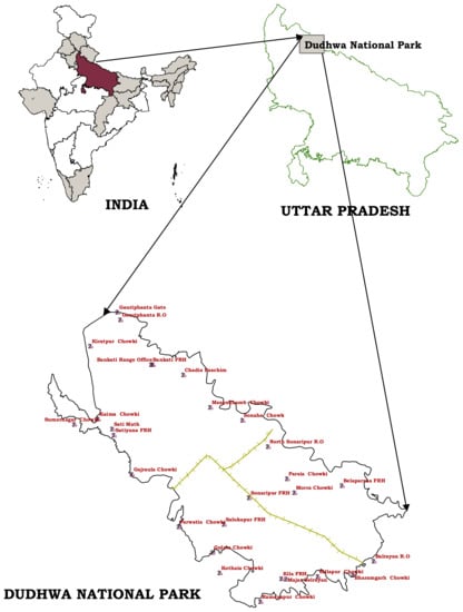
Figure 1.
Location of the study area.
Forest types of the Dudhwa National Park are categorized into four classes and these are named as: northern tropical semi-evergreen forest, northern Indian moist deciduous forest, tropical seasonal swamp forest, and northern tropical dry deciduous forest. The park is mainly dominated by sal (Shorea robusta) trees and the other main flora of the park is shisham (Dalbergia sissoo), jamun (Syzygium cumini), eucalyptus (Eucalyptus globulus), and teak (Tectona grandis) (Figure 2).
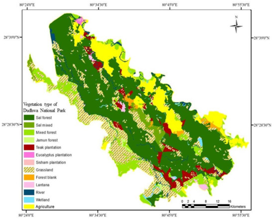
Figure 2.
Forest cover map of the Dudhwa National Park.
This study used field-collected data for 170 plots from different locations and forest vegetation types of the study area [40]. Field data were collected from March 2008 to January 2009 and stratified random sampling with a 0.1 ha plot size was used to collect the field data. Most of the plots were made in the sal forest because sal trees dominated the forest area. In each plot, the data for stem diameter, circumference at breast height (cbh), and tree height were collected. Stem volume estimation was carried with the help Forest Survey of India (FSI)-based volume equations [41]. The stem volume, the specific gravity of the tree species, and biomass expansion factor were used to measure total aboveground biomass. Table 1 shows the number of plots for the field-estimated AGB of different forest types of the national park.

Table 1.
Number of field plots for each forest type.
Figure 3 shows the false color composite of Dudhwa National Park, generated with PolSAR decomposition of the ALOS PALSAR data. The date of acquisition of quad-pol ALOS PALSAR data over the study area was October 31, 2009. Locations of field plots are shown on the Pauli color-coded image derived from L-band quad-pol data in Figure 3.
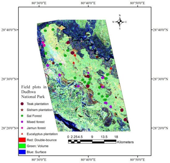
Figure 3.
Field plots in different vegetation type of Dudhwa National Park are shown on the Pauli color-coded image of ALOS PALSAR L-band.
3. Methodology
The methodology adopted to conduct this study is shown in Figure 4. Fully polarimetric ALOS PALSAR data was used to generate the scattering matrix. The shift in POA in the polarization ellipse mainly occurred due to Faraday rotation and structural properties of Earth objects. The initial step of the methodology involved the evaluation and assessment of PolSAR data for the POA shift due to the Faraday rotation. It was expected that the polarimetrically calibrated PolSAR data would not have any effect due to the Faraday rotation, but to assure the quality of the data, FRA estimation and correction was implemented on the single look complex (SLC) data.
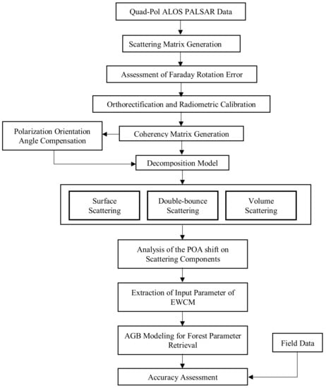
Figure 4.
Methodology flowchart
The Earth’s ionosphere is an anisotropic medium due to the presence of the charged particles in Earth’s persistent magnetic field. The atmospheric propagation of the electromagnetic wave through the ionosphere causes a rotation of polarization plane, and finally a shift in the POA occurs due to the Faraday rotation. The possible effects in PolSAR data due to the Faraday rotation are [20,42,43]:
- Reciprocity does not hold.
- Error in the estimation of calibration distortion.
- Polarimetric-decomposition-based scattering retrieval can be affected.
The polarimetric distortion matrix considering the Faraday rotation error is estimated as follows [20,44]:
where, M is the scattering matrix having a Faraday rotation error but is free from all other polarimetric distortions; S is the scattering matrix free from all polarimetric distortions including the Faraday rotation error, which needs to be derived; and Ω is the Faraday rotation angle by which the polarization plane of the electromagnetic (EM) wave is rotated in the Ionosphere.
The circularly polarized EM waves are not affected by the Faraday rotation effect, so for estimating the Faraday rotation angle, the linearly polarized EM can be converted to the circular basis and the distortions existing in the circular basis scattering matrix can be evaluated as follows [20,44,45]:
where refers to left circular transmitted:left circular received EM waves, refers to left circular transmitted:right circular received EM waves, refers to right circular transmitted:left circular received EM waves, refers to right circular transmitted:right circular received EM waves, and .
After estimating the circularly polarized scattering matrix elements, the Faraday rotation angle is estimated as follows [44]:
After estimating the Faraday rotation angle Ω using Equation (3), it is substituted into Equation (1) to derive the scattering matrix free from the Faraday rotation error.
To minimize the slant range ambiguity of the SAR data and have the actual ground information of the features within the scene, the orthorectification was performed using the range doppler orthorectification method [46]. The radiometric calibration was implemented on the SAR data to get the actual radar cross-section associated with different polarimetric channels. The Sentinel Application Platform (SNAP 6.0) [47] was used for radiometric calibration and orthorectification of the SAR data. The orthorectified and radiometrically calibrated polarimetric combinations were used to generate a 2 × 2 scattering matrix. The scattering matrix was used to identify the scattering behavior of objects after interaction with the electromagnetic wave. This matrix was represented using a systematic combination of horizontal and vertical polarization states of the transmitted and received signals:
The coherency matrix is a second-order derivative of the scattering matrix that is derived from matrix multiplication of the Pauli feature vector with its own trans-conjugate. The six elements of the coherency matrix of the monostatic SAR system are aligned in a way to make the coherency matrix a Hermitian matrix. The elements of the upper triangular portion of the coherency matrix are equal in amplitude and these elements are the complex conjugate of the corresponding elements of the lower triangular portion. The diagonal elements of the matrix represent the total power or span of the matrix. The representation of scattering information in terms of first- and second-order derivatives by defining a target vector is more convenient in comparison to the scattering matrix [48]. The requirement of second-order derivatives or a coherency-matrix-based decomposition modeling depends on the heterogeneity in the scattering nature of the targets within a resolution cell of the SAR data [49,50]. Mainly two modeling approaches have been widely used and these are coherent and incoherent decomposition models [51,52,53]. The coherent decomposition models are mainly based on the first-order derivatives of the scattering matrix and they provide good results in the scattering identification if the heterogeneity in the SAR resolution cell is low. An increase in the heterogeneity of the scatterers in the imaged area requires a higher order of scattering retrieval, which includes the combinations of co-polarized and cross-polarized channels of the SAR data [54]. Thus, the coherency-matrix-based decomposition model was used to retrieve scattering from the forest vegetation of Dudhwa National Park. The noise in the SAR data due to speckle could not be directly removed from the scattering matrix. Generally, all the polarimetric speckle-filtering approaches are implemented on the coherency or covariance matrix. The polarimetric boxcar speckle filtering approach was performed on the 3 × 3 coherency matrix to minimize the effect of speckle from the PolSAR data. It was found that the decomposition-model-based scattering information retrieval suffered from an overestimation of volume scattering and underestimation of double-bounce scattering due to a shift in the polarization orientation angle (POA) of the polarization ellipse of the electromagnetic wave. The shift in polarization orientation angle (POA) is induced due to the azimuth slope, Faraday rotation, and target geometry [55,56,57]. This study focused on the estimation and compensation of POA shift in PolSAR data that was caused by the azimuth slope and target geometry. Lee et al. (2000) had proposed two approaches to compensate for the POA shift [58]. In the first method, the digital elevation model was used, and in the second approach, POA was derived from the PolSAR scattering matrix. The study recommended the implementation of POA compensation with the PolSAR-scattering-matrix-based approach [58]. The purpose of the deorientation process is to remove the ambiguity in the scattering mechanism induced due to randomly distributed target orientation angles, and it can make two similar objects with different orientation angles due to the difference in geometric shape and structure yield the same scattering behavior after decomposition modeling. Hence, the deorientation should be applied to the PolSAR data before they are decomposed into three scattering components. To overcome this limitation of decomposition modeling, POA compensation was implemented by the unitary transformation and rotation of the coherency matrix. The coherency matrix after POA correction may be represented as Equation (5):
The coherency-matrix-based decomposition was performed to retrieve different scattering elements from a single resolution cell of the SAR data.
3.1. Decomposition Model
The Yamaguchi four-component scattering model [17] expands the coherency matrix in four elements, as shown in Equation (6):
The coherency matrix elements to represent the surface, double-bounce, volume, and helix scatterings are represented by Tsurface, Tdouble, Tvolume, and Thelix, respectively, and their scattering powers are Ps, Pd, Pv, and Ph. Figure 5a shows the surface scattering in which all the incident radiation from the SAR sensor was reflected away from the direction of sensors in such a way that the sensor receives minimum or negligible backscatter signal contributed by the ground. These features appeared dark in comparison to other complex structures. The double-bounce scattering is shown in Figure 5b, which was obtained from ground–stem or stem–ground interaction in the forest area. The scattering, which was contributed by the entire volume of the structure, was mainly obtained from forest vegetation and is known as volume scattering (Figure 5c). The helix scattering is a special case of volume scattering in which SAR signals are returned from the helical shape of the object, as shown in Figure 5d.
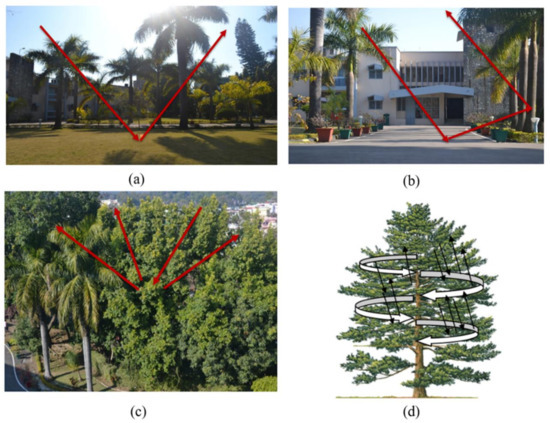
Figure 5.
Four component decomposition of scattering powers: (a) surface scattering, (b) double-bounce scattering, (c) volume scattering, and (d) helix scattering [59,60].
Since in the forest area, helix scattering was obtained as a special scattering pattern from forest vegetation, the helix scattering and volume scattering were merged and the combined scattering pattern was represented as the scattering from vegetation (). The scattering contributed by ground was represented as surface scattering () and ground–stem interaction was retrieved from the double-bounce scattering pattern ().
The coherency matrix elements for surface, double-bounce, volume, and helix scattering are shown in the Figure 6 in different colors. The coefficients α and w for double-bounce and surface scattering elements, respectively, are determined to generate their coherency matric elements. The volume scattering element of Yamaguchi et al. (2011) [17] is based on the magnitude balance of HH and VV polarimetric channels of the scattering matrix, as shown in Figure 6 and Equation (7):
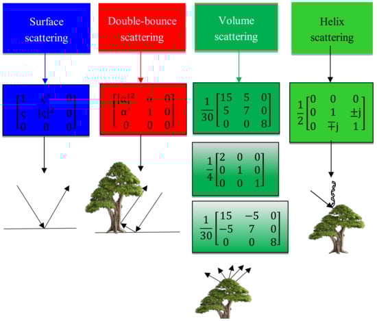
Figure 6.
Scattering elements of the Yamaguchi four component decomposition [17].
The scattering elements retrieved from four component decomposition of ALOS PALSAR data is shown in the Figure 7. It is clearly visible from Figure 7a and Figure 8 that the contribution in scattering due to smooth surfaces was highlighted in the surface scattering element of the decomposition output. The surface scattering element was highlighted in a blue color in a false-color composite (FCC) image of the four component decomposition of Yamaguchi model. The two rivers located in the northeast and southwest portion of Figure 7 and Figure 8 are highlighted in a blue color due to the dominance of surface scattering from these features. The forest vegetation of the Dudhwa National Park provided a dominance of volume scattering; as a result, the area of land covered by vegetation was highlighted in the volume scattering image (Figure 7c). It is evident in Figure 7a that the amount of surface scattering in the forest area was much smaller. Less surface scattering from the forest vegetation indicates that the long wavelength of the L-band SAR system penetrated through the canopy and it was able to interact with all of the components (leaves, twigs, branches, stem of the tree) of the forest vegetation. The presence of double-bounce scattering elements could be easily detected in the forest area as bright patches at several locations in Figure 7b. The dominance of volume and double-bounce scattering elements could also be seen at several locations in SAR imagery as pink and yellow colors in the FCC image (Figure 8) of the decomposition result.
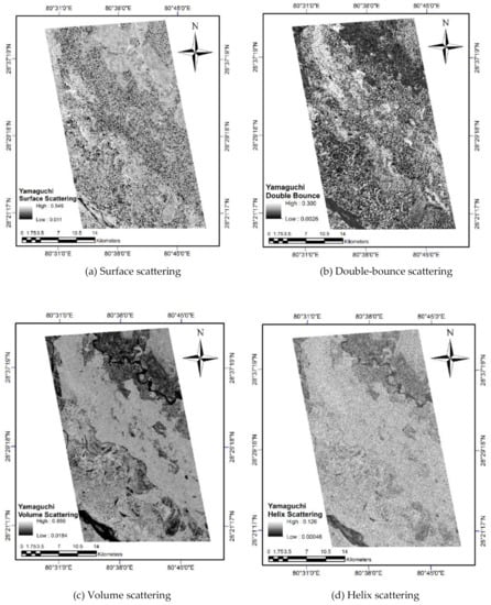
Figure 7.
Four-component decomposition of the ALOS PALSAR data.
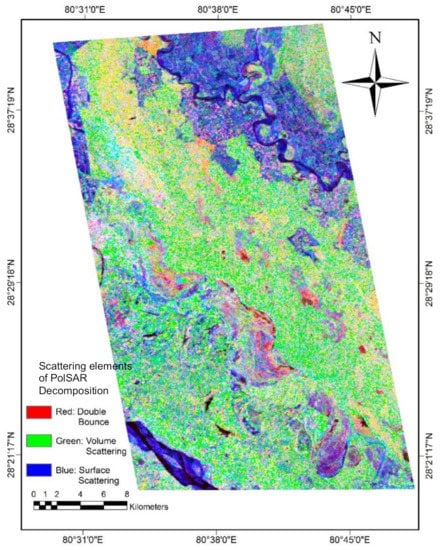
Figure 8.
False-color composite of the scattering elements of the ALOS PALSAR data.
3.2. Scattering of Electromagnetic Waves from Forest Vegetation
Figure 9 shows all the possible types of scattering of SAR electromagnetic waves with forest vegetation. The concept of the water cloud model (WCM) was given by Attema and Ulaby (1978) [61], where the model was developed from the concept of total backscatter of a SAR signal as a combination of different scattering elements contributed by the ground and vegetation. The WCM was developed on the assumption of vegetation as water droplets that behaves like a cloud of water droplets over the ground. The model assumes the uniform distribution of water droplets, which is not the real scenario in any forest vegetation. The limitation of this assumption was compensated for in this work by including the modeling approach of randomly oriented dipoles for scattering retrieval from forest vegetation using fully polarimetric SAR-based decomposition. The conventional WCM model assumes a similar type of scattering of electromagnetic waves from water droplets uniformly distributed in the vegetation slab. The conventional WCM was modified by Santoro et al. (2002) [62] to describe the usefulness of the model for forest parameter retrieval. The model assumes that the total incident radiation on the forest vegetation will have two components: one will be directly returned towards the sensors after scattering and the second portion will penetrate through the attenuating layer of the forest structure to represent the scattering contributed by forest vegetation.
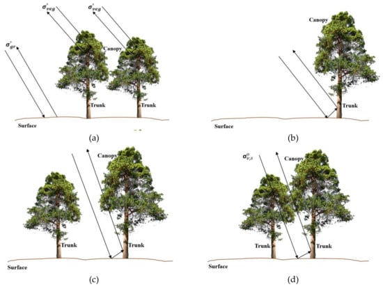
Figure 9.
Interaction of electromagnetic waves with forest vegetation: (a) water cloud model, (b) ground–stem interaction from canopy gaps, (c) ground–stem interaction through the canopy, (d) canopy volume scattering to the ground and further scattering through the canopy.
The simplest form of a water cloud model in terms of scattering contribution of vegetation and the ground within a single SAR resolution cell is written as [63]:
where is the total backscatter observed from single SAR resolution, is the contribution in the backscatter due to forest vegetation, is the contribution in the backscatter due to the ground in the corresponding resolution cell, and is the two-way tree transmissivity of the electromagnetic wave through the forest canopy.
The model shown in Equation (8) does not include the canopy gap. However, in a real scenario, the possibility of the returned signal of electromagnetic waves through canopy gaps is very high for the locations within forest patches where the forest density is low. The WCM was again modified to include the canopy gaps in the modeling for the forest parameter retrieval and it is shown in Equation (9) [64]:
where η is the area fill factor. The first element of Equation (9) represents the contribution in the scattering from the ground through the gaps between the forest vegetation. The fraction of the ground in the SAR resolution cell covered by forest vegetation is termed as the area fill factor and is represented as η. The fraction of ground not covered by the forest vegetation is represented by (1 − η). The (1 − η) shows the portion of the ground that contributes to the scattering with the attenuation in the electromagnetic wave as per the available fraction of the ground not covered by the forest vegetation. The second element of Equation (9) is and it represents the portion of backscatter contribution in the total scattering due to the ground backscatter with the attenuation of the electromagnetic waves through a forest canopy. The last element of the Equation (9) is and it represents the backscattering through vegetation layer with a transmissivity of the electromagnetic waves of less than one. If the transmissivity becomes one, then the scattering component contributed by forest vegetation will become zero and the scattering from the ground contributed in the presence and absence of attenuating layers will be available. The term expresses the transmissivity of the electromagnetic wave through a forest canopy.
The total transmissivity of the electromagnetic wave through the attenuating layer of the forest vegetation is expressed as the exponent of the total attenuation in the electromagnetic waves due to the two-way propagation through the attenuating media “α” and the thickness of the attenuating layer “h”:
Generally, within the resolution cell, it is difficult to represent transmissivity for a single tree. A SAR resolution cell may cover several trees, and to overcome this limitation, the term forest transmissivity was used to represent two-way transmissivity of the electromagnetic wave. The forest transmissivity of the electromagnetic waves in the presence of an attenuating layer of thickness “h” is represented by Equation (10). The two-way forest transmissivity of the electromagnetic waves through the forest canopy can be expressed in terms of the aboveground biomass “B” and an empirically defined coefficient “β” [37,65], as shown in Equation (11):
The total backscatter of the resolution cell for forest can be expressedas Equation (12).
The aboveground biomass can be easily retrieved from the inversion of Equation (12). To retrieve AGB for a particular resolution cell with known SAR backscatter parameters, Equation (12) may be written as:
The L-band, due to its high penetration capabilities, also interacts with the trunk and ground. Therefore, there is a need for considering these higher order interactions.
3.3. Methods for Implementation for Higher Order Scattering Mechanisms
This section deals with all the possible interactions of electromagnetic waves for scattering information retrieval. All four scattering possibilities with a single resolution cell are discussed to retrieve the scattering contribution from different scatterers for AGB estimation.
Backscattering from the ground–stem interaction from the canopy gaps, as shown in Figure 9b, is represented as:
In Equation (14), represents the fraction of the ground not covered by the canopy and is the backscattering from the ground–stem interaction.
The scattering contribution of the ground–stem interaction through the canopy is represented by Equation (15):
The forward scattering of volume scattering from the canopy to the ground and further canopy scattering is related to the volume scattering coefficient and attenuation of an electromagnetic wave through the forest vegetation [66]. The forest canopy to ground forward scattering through the attenuating vegetation layer (Figure 9d) is represented by . The halfway attenuation parameter to represent the ground–stem interaction in Figure 9c may be represented by . Therefore, the water cloud model, which is extended for higher order interactions from the decomposition of fully polarimetric SAR data, is obtained from Equations (9), (14), and (15):
The halfway attenuation power for ground–stem scattering is a special condition of stem–ground scattering mechanism weighted by area fill factor; therefore, there is no requirement to include an additional term for this scattering component. The volume scattering component () will be exactly equal to if the transmissivity through canopy is zero. The volume scattering component was retrieved from the volume and helix scattering elements obtained from Equation (7) and Figure 6. The sum of the volume scattering and helix scattering was taken to represent the total scattering contributed by the forest canopy. After considering these facts, the extended water cloud model can be represented as Equation (17):
Equation (17) can be expressed in the terms of alpha and attenuating layer:
where can be substituted [37] with a two-way forest transmissivity :
The equation of EWCM can be written as Equation (20), where “” is an empirically defined coefficient and “B” is the AGB:
Unknown parameters of EWCM are the backscattering contributed by ground (, backscattering from forest vegetation (, backscattering due to ground stem interaction (), and the coefficient (β). Polarimetric decomposition modeling provides the capability to retrieve these parameters as scattering values from single a SAR resolution cell. The parameters of the EWCM could be easily retrieved from the scattering elements shown in Equation (7).
4. Results and Discussions
4.1. Estimation of the Faraday Rotation Angle (FRA) of ALOS PALSAR PolSAR Data
The shift in FRA due to the rotation of the polarization plane along the direction of propagation of electromagnetic wave was estimated and the correction was implemented according to Equations (1)–(3). Figure 10 shows the image of the FRA retrieved from ALOS PALSAR data for the study area. It could be easily seen that the shift in the polarization orientation angle due to the Faraday rotation was approximately zero for most of the locations of the PolSAR data. Figure 10a shows the Faraday rotation angle (Ω) before compensation. By analyzing the image, it can be clearly observed that the Faraday rotation angle ranged from −0.8 to 0.8 degrees, indicating a negligible Faraday rotation error in the dataset. Figure 10b shows the Faraday rotation angle after compensation using the methodology described above. It can be observed that there was no change between Figure 10a and Figure 10b, indicating the residual Faraday rotation error was at its lowest level of minimization.
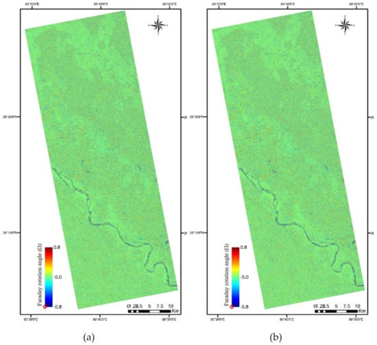
Figure 10.
Faraday rotation angle image: (a) before compensation, and (b) after compensation.
Figure 11a shows the histogram of the Faraday rotation angle image before compensation. From the figure, it can be seen that the mean Faraday rotation angle was 0.00801 degrees with a standard deviation of only 0.160 degrees, indicating a negligible Faraday rotation error. Figure 11b shows the histogram of the Faraday rotation angle after compensation. It can be seen in Figure 11b that the mean Faraday rotation angle was 0.00643 degrees with a reduction of only 0.0015 from the mean Faraday rotation angle before compensation and the standard deviation was now 0.156 degrees. From all these values, it can be clearly said that the ALOS PALSAR dataset was accurately compensated to account for the Faraday rotation error by the Japan Aerospace Exploration Agency (JAXA) before data dissemination and there is no requirement to perform an additional Faraday rotation error compensation to the datasets.
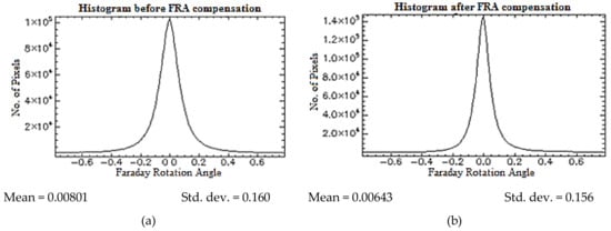
Figure 11.
Histogram of the Faraday rotation angle (Ω) image: (a) before compensation, and (b) after compensation.
4.2. Regression between the Field-Estimated Aboveground Biomass (AGB) and Volume Scattering
Regression between the volume scattering obtained from PolSAR decomposition of the SAR data for forest area was carried to see the effect of deorientation on volume scattering for 170 plots of Dudhwa National Park where the field data were collected from. Figure 12 shows a comparison of the volume scattering values for all of the 170 forest plots for which field data were collected. A decrease in volume scattering after deorientation was noted for all of the plots.
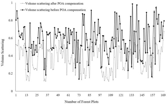
Figure 12.
Comparison of volume scattering values (before and after deorientation of coherency matrix) for all of the 170 forest plots for which field data were collected.
Linear regression between the volume scattering component and field-inventory-based aboveground biomass is shown in Figure 13a,b.
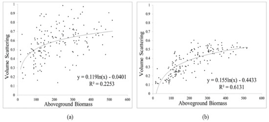
Figure 13.
Regression between AGB and volume scattering obtained from: (a) PolSAR decomposition before deorientation of coherency matrix, and (b) PolSAR decomposition after deorientation of the coherency matrix.
The increased value of the coefficient of determination (R2) was obtained from the regression between the field-observed AGB and the volume scattering obtained after deorientation. The coefficient of determination obtained from the regression between AGB and volume scattering obtained from deorientation of the coherency matrix showed a better R2 (0.61) in comparison to regression of the AGB with volume scattering without a deorientation of the coherency matrix.
4.3. PolSAR Based Modeling for Forest Biomass Retrieval
Four parameters—backscatter from the ground (σ0gr), backscatter from the vegetation (σ0veg), stem–ground interaction of the electromagnetic wave (σ0gs), and the empirically defined coefficient (β)—of the extended water cloud model are unknown. These unknown parameters were retrieved from the polarimetric decomposition of the SAR data. Backscatter from ground (σ0gr) was retrieved from the surface scattering component of the PolSAR decomposition modeling, and scattering contributed by the vegetation was modeled as randomly oriented dipoles and retrieved from the volume scattering component. The contribution in scattering due to the ground–stem interaction was retrieved from the double-bounce scattering component of the decomposed output of the PolSAR data.
The backscattering parameters of EWCM were taken with respect to the scattering from different targets in terms of volume, surface, and double-bounce scattering. The field-measured AGB for 170 plots of Dudhwa National Park area was used in the study. The unknown parameters of EWCM were reduced to one, which was the empirically defined coefficient “β” after using the polarimetric decomposition output as the input parameter for the respective backscattering:
Equation (21) was used to retrieve the unknown coefficient and it can be written in terms of the scattering coefficients for the retrieval of β. The input of backscatter values contributed by vegetation, ground, ground–stem interaction, and AGB was used to calculate an average value of β. The β was calculated for 50 plots and an average value of “β” was further used in modeling the AGB for the remaining plots. Since the study area was dominated by sal forest, most of the plots (30 plots) were taken from sal forest. A total of six plots from the mixed forest, six plots from a teak plantation, four plots from a sisham forest, two plots from a eucalyptus plantation, and two from a jamun forest were considered for the β estimation.
The AGB “B” was modeled by inverting Equation (22) of the EWCM. The average value of β was used in the modeling approach (Equation (21)) for the AGB estimation. POA-shift-compensated results of the four component Yamaguchi decomposition model [17] was used as input model parameters to retrieve scattering from the ground, vegetation, and ground–stem interaction to retrieve the forest AGB. Backscattering components of the EWCM were taken from POA-compensated PolSAR data. Equation (20) was inverted to retrieve the AGB, as shown in Equation (22):
Backscattering power, along with the empirically defined coefficient β, was used in Equation (21) measure AGB “B” in tons/ha. The modeled AGB “B” and field-measured AGB were used to build a scatterplot. The best fit line shows the correlation between the model AGB and field-estimated AGB. The scatterplot shown in Figure 14 illustrates the agreement between the plot-wise distribution of the modeled and ground-measured AGB. The coefficient of determination, as observed from the regression, showed acceptable variability in the AGB estimates obtained from the extended water cloud model. The term “acceptable variability” considers the strength of the SAR wave for a dense tropical forest, noise in the backscatter image, and the saturation condition. The variability of the estimates was explained in terms of the spread of the AGB estimates, as observed from the scatterplot between the modeled and ground-measured AGB. As shown in Figure 14, the model achieved a 0.78 coefficient of determination in the AGB estimation.
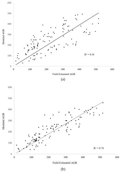
Figure 14.
Relationship between the field-estimated AGB and the modeled AGB: (a) before POA compensation, and (b) after POA compensation.
To evaluate the model performance to describe the results of the forest AGB retrieval, two statistical parameters are commonly considered: the first is the coefficient of determination R2 and the second is the root mean square error (RMSE). Ground-truth measurements at plot level were highly accurate; therefore, the correction for sampling errors was not needed. From Figure 14a,b, it is evident that the coefficient of determination increased after POA compensation of the SAR data. Without POA compensation, the regression between the field-measured AGB and modeled AGB was 0.36, and after POA compensation, an increased value (0.78) was obtained. Based on the regression between the backscatter and AGB taking into account the behaviour of electromagnetic waves, the retrieved output for the AGB obtained from the model was shown to be capable of measuring forest AGB. The root mean square error observed for the plots in the AGB retrieval was 92.90 tons/ha before POA compensation and 59.77 tons/ha was obtained through the EWCM after compensation for the POA.
This study has utilized the polarimetric-decomposition-based parameter in EWCM modeling approaches. Previous studies carried out with SAR-based modeling for forest AGB retrieval has shown promising results. Michelakis et al. (2015) carried out a woody biomass estimation with L-band SAR-backscatter-based water cloud model and the retrieved R2 and RMSE were 0.70 and 25 tons/ha, respecitively [67]. Another study was carried by Santi et al. (2017) to retrieve the forest growing stock volume (SV) using a multifrequency SAR-based WCM approach [68]. A correlation of 0.86 and RMSE of 77 m3/ha was obtained in the growing SV measurement. Peregan and Yamagata (2013) utilized an L-band SAR-based study over the forest area of western Siberia for AGB estimation using WCM [69]. The range of RMSE for AGB estimation for the Siberian forest was 46–55 tons/ha.
An effort had been made to analyze the linear regression between field-measured AGB and EWCM-based modeled output of AGB after POA compensation of the SAR data. The coefficient of determination through the linear regression and RMSE for different forest types can be easily seen in Figure 15a–f and Table 2. It was observed that the mixed forest showed the highest R2 (0.86) with a minimal RMSE (17.58 tons/ha). A high RMSE (74.02 tons/ha) was obtained for the teak plantation and a minimal R2 was recorded for the eucalyptus plantation.
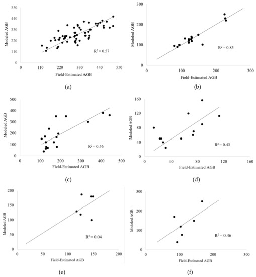
Figure 15.
Relationship between the field-estimated AGB and the modeled AGB for: (a) sal forest and mixed sal forest, (b) mixed forest, (c) teak plantation, (d) sisham plantation, (e) eucalyptus plantation, and (f) jamun forest.
Table 2.
Coefficient of determination and RMSE for the AGB estimation of different forest types of Dudhwa National Park, Uttar Pradesh, India.
Although a very low RMSE and very high R2 is not evident from Figure 14 and Figure 15, this result for the modeled output can still be considered satisfactory, since the PolSAR-based EWCM has shown very little dependency on field measurements to retrieve model parameters for AGB modeling. The biomass map was generated from the PolSAR-based EWCM and it is shown in Figure 16. From Figure 16, it is clearly visible that grasslands (blue color) showed much less AGB and a higher biomass can be obtained for the dense forest area represented by the red color in the image. The modeled output map for the study area shows a maximum of 531 tons/ha AGB as can be easily seen from the AGB map.
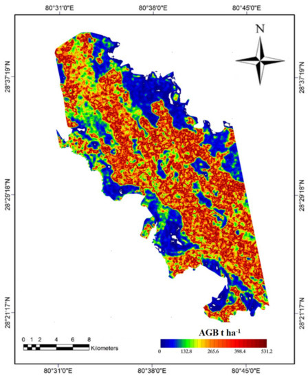
Figure 16.
Aboveground biomass map generated from PolSAR-based extended water cloud model.
5. Conclusions
The prime focus of the present study was a PolSAR-based framework to implement a semiempirical model EWCM for forest AGB estimation. The study also analyzed the effect of POA compensation on a decomposition-based scattering retrieval and AGB estimation.
Measurement of each individual scatterer’s contribution in a SAR resolution cell was the biggest problem and the procedure to retrieve the scattering of vegetation and ground from single- or dual-polarized data was tedious. Polarimetric SAR data was used as a solution to retrieve different scatterers to include higher order scattering elements in modeling approaches to retrieve forest AGB. A framework for polarimetry-based higher order scattering information retrieval for a semiempirical model EWCM was successfully implemented for forest AGB retrieval. The proposed EWCM showed a lower dependency on field data for model parameter retrieval. The potential of polarimetric SAR-data-based semi-empirical modeling for forest aboveground biomass estimation was evaluated with the help of field-collected data.
Based on the results obtained from decomposition models, the study concludes that the volume scattering component of the forest area obtained from the Yamaguchi model was overestimated due to the shift in POA. After compensation of the POA shift, a decrease in volume scattering was recorded. A better regression between volume scattering and the AGB was retrieved after deorientation of the coherency matrix. A deorientation technique to compensate POA shift improved the potential of polarimetric SAR data for identification of the nature of scatterers. An improvement in AGB estimation through EWCM was obtained after POA compensation of the coherency matrix. Without deorientation of the PolSAR coherency matrix, EWCM showed a modeled AGB of 92.90 tons/ha and a 0.36 R2 was recorded through linear regression between the field-measured AGB and modeled output. After deorientation of PolSAR data, an increased R2 (0.78) with a lower RMSE (59.77 tons/ha) was obtained as an output of EWCM. The study strongly recommends the deorientation procedure before polarimetric decomposition to minimize the problem of overestimation of volume scattering and underestimation of double-bounce scattering. PolSAR-based modeling provides the potential to retrieve a different scattering component with reliable accuracy and it provides a lower dependency on field data to optimize model parameters for AGB estimation.
Author Contributions
Conceptualization, S.K.; methodology, S.K.; software, S.K. and H.G.; validation, S.K., R.D.G. and S.P.S.K.; formal analysis, S.K.; investigation, S.K.; resources, S.K. and S.P.S.K.; data curation, S.K. and S.P.S.K.; writing—original draft preparation, S.K.; writing—review and editing, S.K., R.D.G. and S.P.S.K.; visualization, S.K.; supervision, R.D.G. and S.P.S.K.; project administration, S.K., R.D.G., H.G. and S.P.S.K.; funding acquisition, H.G. and S.K.
Funding
This paper is financially supported by Space Application Centre, Ahmedabad, India, grant F. No: EPSA/3.1.1/2017.
Acknowledgments
The authors are very grateful for the creative research effort of the whole research team of ESA for providing SNAP 6.0 and PolSARPro 4.2 tools for polarimetric processing of the SAR data.
Conflicts of Interest
The authors declare no conflict of interest.
References
- Falk, A.; Gerald, B.; Adrian, B.; Sean, B.; Susan, C.; Manab, C.; Bruce, C.; Anup, D.; Andrea, D.; Ralph, D.; et al. NASA-ISRO SAR (NISAR) Mission Science Users’ Handbook, 1st ed.; Jet Propulsion Laboratory, California Institute of Technology: California, CA, USA, 2018. [Google Scholar]
- Sinha, S.; Jeganathan, C.; Sharma, L.K.; Nathawat, M.S. A review of radar remote sensing for biomass estimation. Int. J. Environ. Sci. Technol. 2015, 12, 1779–1792. [Google Scholar] [CrossRef]
- Timothy, D.; Onisimo, M.; Cletah, S.; Adelabu, S.; Tsitsi, B. Remote sensing of aboveground forest biomass: A review. Trop. Ecol. 2016, 57, 125–132. [Google Scholar]
- Shi, L.; Liu, S. Methods of Estimating Forest Biomass: A Review. In Biomass Volume Estimation and Valorization for Energy; Tumuluru, J.S., Ed.; InTech: Rijeka, Croatia, 2017; pp. 23–46. [Google Scholar]
- Manolis, E.N.; Zagas, T.D.; Poravou, C.A.; Zagas, D.T. Biomass assessment for sustainable bioenergy utilization in a Mediterranean forest ecosystem in northwest Greece. Ecol. Eng. 2016, 91, 537–544. [Google Scholar] [CrossRef]
- Suzuki, R.; Kim, Y.; Ishii, R. Sensitivity of the backscatter intensity of ALOS/PALSAR to the above-ground biomass and other biophysical parameters of boreal forest in Alaska. Polar Sci. 2013, 7, 100–112. [Google Scholar] [CrossRef]
- Mitchard, A.; Saatchi, S.; Woodhouse, I.H.; Nangendo, G.; Ribeiro, S.; Williams, M.; Ryan, M.; Lewis, S.L.; Feldpausch, T.R.; Meir, P. Using satellite radar backscatter to predict above-ground woody biomass: A consistent relationship across four different African landscapes. Geophys. Res. Lett. 2009, 36, 1–6. [Google Scholar] [CrossRef]
- Dobson, M.C.; Ulaby, F.T.; LeToan, T.; Beaudoin, A.; Kasischke, E.S.; Christensen, N. Dependence of radar backscatter on coniferous forest biomass. IEEE Trans. Geosci. Remote Sens. 1992, 30, 412–415. [Google Scholar] [CrossRef]
- Letoan, T.; Beaudoin, A.; Riom, J.; Guyon, D. Relating Forest Biomass to SAR Data. IEEE Trans. Geosci. Remote Sens. 1992, 30, 403–411. [Google Scholar] [CrossRef]
- Rodriguez-Veiga, P.; Wheeler, J.; Louis, V.; Tansey, K.; Balzter, H. Quantifying Forest Biomass Carbon Stocks From Space. Curr. For. Rep. 2017, 3, 1–18. [Google Scholar] [CrossRef]
- Santoro, M.; Cartus, O. Research Pathways of Forest Above-Ground Biomass Estimation Based on SAR Backscatter and Interferometric SAR Observations. Remote Sens. 2018, 10, 608. [Google Scholar] [CrossRef]
- Santoro, M.; Beer, C.; Cartus, O.; Schmullius, C.; Shvidenko, A.; McCallum, I.; Wegmüller, U.; Wiesmann, A. Retrieval of growing stock volume in boreal forest using hyper-temporal series of Envisat ASAR ScanSAR backscatter measurements. Remote Sens. Environ. 2011, 115, 490–507. [Google Scholar] [CrossRef]
- Ningthoujam, R.K.; Balzter, H.; Tansey, K.; Feldpausch, T.R.; Mitchard, E.T.A.; Wani, A.A.; Joshi, P.K. Relationships of S-band radar backscatter and forest aboveground biomass in different forest types. Remote Sens. 2017, 9, 1116. [Google Scholar] [CrossRef]
- Lee, J.S.; Pottier, E. Polarimetric Radar Imaging: from Basics to Applications; CRC Press: Boca Raton, FL, USA, 2009; ISBN 978-1-4200-5497-2. [Google Scholar]
- Polarimetry—NASA-ISRO SAR Mission (NISAR). Available online: https://nisar.jpl.nasa.gov/technology/polsar/ (accessed on 23 May 2018).
- Sato, A.; Yamaguchi, Y.; Singh, G.; Park, S.-E. Four-component scattering power decomposition with extended volume scattering model. IEEE Geosci. Remote Sens. Lett. 2012, 9, 166–170. [Google Scholar] [CrossRef]
- Yamaguchi, Y.; Sato, A.; Boerner, W.M.; Sato, R.; Yamada, H. Four-Component Scattering Power Decomposition With Rotation of Coherency Matrix. IEEE Trans. Geosci. Remote Sens. 2011, 49, 2251–2258. [Google Scholar] [CrossRef]
- Lee, J.S.; Ainsworth, T.L. The effect of orientation angle compensation on coherency matrix and polarimetric target decompositions. IEEE Trans. Geosci. Remote Sens. 2011, 49, 53–64. [Google Scholar] [CrossRef]
- Souissi, B.; Ouarzeddine, M. Analysis of Orientation Angle Shifts on the Polarimetric Data Using Radarsat2 Images. IEEE J. Sel. Top. Appl. Earth Obs. Remote Sens. 2016, 9, 1331–1342. [Google Scholar] [CrossRef]
- Shimada, M. Imaging from Spaceborne and Airborne SARs, Calibration, and Applications, 1st ed.; CRC Press: Boca Raton, FL, USA, 2018; ISBN 9781315282619. [Google Scholar]
- Lee, J.S.; Schuler, D.L.; Ainsworth, T.L.; Krogager, E.; Kasilingam, D.; Boerner, W.M. On the estimation of radar polarization orientation shifts induced by terrain slopes. IEEE Trans. Geosci. Remote Sens. 2002, 40, 30–41. [Google Scholar]
- Gonçalves, F.G.; Santos, J.R.; Treuhaft, R.N. Stem volume of tropical forests from polarimetric radar. Int. J. Remote Sens. 2011, 32, 503–522. [Google Scholar] [CrossRef]
- Zhang, H.; Wang, C.; Zhu, J.; Fu, H. Forest Above-ground Biomass Estimation for Rugged Terrain by Using ESAR Polarization Data. Cehui Xuebao/Acta Geod. Cartogr. Sin. 2018, 47, 1353–1362. [Google Scholar]
- Golshani, P.; Maghsoudi, Y.; Sohrabi, H. Relating ALOS-2 PALSAR-2 Parameters to Biomass and Structure of Temperate Broadleaf Hyrcanian Forests. J. Indian Soc. Remote Sens. 2019, 47, 749–761. [Google Scholar] [CrossRef]
- Huang, X.; Ziniti, B.; Torbick, N.; Ducey, M.J. Assessment of forest above ground biomass estimation using multi-temporal C-band Sentinel-1 and Polarimetric L-band PALSAR-2 data. Remote Sens. 2018, 10, 1424. [Google Scholar] [CrossRef]
- Tomar, K.S.; Kumar, S.; Tolpekin, V.A.; Joshi, S.K. Semi-empirical modelling for forest aboveground biomass estimation using hybrid and fully PolSAR data. In Proceedings of the SPIE—The International Society for Optical Engineering, Baltimore, MD, USA, 17–21 April 2016; Volume 9877. [Google Scholar]
- Kumar, S.; Khati, U.G.; Chandola, S.; Agrawal, S.; Kushwaha, S.P.S. Polarimetric SAR Interferometry based modeling for tree height and aboveground biomass retrieval in a tropical deciduous forest. Adv. Sp. Res. 2017, 60, 571–586. [Google Scholar] [CrossRef]
- Cassol, L.H.; Carreiras, M.J.; Moraes, C.E.; Aragão, E.L.; Silva, V.C.; Quegan, S.; Shimabukuro, E.Y. Retrieving Secondary Forest Aboveground Biomass from Polarimetric ALOS-2 PALSAR-2 Data in the Brazilian Amazon. Remote Sens. 2018, 11, 59. [Google Scholar] [CrossRef]
- Pereira, O.L.; Furtado, F.L.; Novo, M.E.; Sant’Anna, J.S.; Liesenberg, V.; Silva, S.T. Multifrequency and Full-Polarimetric SAR Assessment for Estimating Above Ground Biomass and Leaf Area Index in the Amazon Várzea Wetlands. Remote Sens. 2018, 10, 1655. [Google Scholar] [CrossRef]
- Svoray, T.; Shoshany, M. SAR-based estimation of areal aboveground biomass (AAB) of herbaceous vegetation in the semi-arid zone: A modification of the water-cloud model. Int. J. Remote Sens. 2002, 23, 4089–4100. [Google Scholar] [CrossRef]
- Chuah, H.T.; Tan, H.S. A radar backscatter model for forest stands. Waves Random Media 1992, 2, 7–28. [Google Scholar] [CrossRef]
- Santoro, M.; Eriksson, L.E.B.; Fransson, J.E.S. Reviewing ALOS PALSAR backscatter observations for stem volume retrieval in Swedish forest. Remote Sens. 2015, 7, 4290–4317. [Google Scholar] [CrossRef]
- Behera, M.; Tripathi, P.; Mishra, B.; Kumar, S.; Chitale, V.; Behera, S.K. Above-ground biomass and carbon estimates of Shorea robusta and Tectona grandis forests using QuadPOL ALOS PALSAR data. Adv. Sp. Res. 2015, 57, 552–561. [Google Scholar] [CrossRef]
- Santoro, M.; Wegmüller, U.; Askne, J. Forest stem volume estimation using C-band interferometric SAR coherence data of the ERS-1 mission 3-days repeat-interval phase. Remote Sens. Environ. 2018, 216, 684–696. [Google Scholar] [CrossRef]
- Pulliainen, J.T.; Kurvonen, L.; Hallikainen, M.T. Multitemporal behavior of L-and C-band SAR observations of boreal forests. IEEE Trans. Geosci. Remote Sens. 1999, 37, 927–937. [Google Scholar] [CrossRef]
- Ranson, K.J.; Sun, G.; Weishampel, J.F.; Knox, R.G. Forest biomass from combined ecosystem and radar backscatter modeling. Remote Sens. Environ. 1997, 59, 118–133. [Google Scholar] [CrossRef]
- Kumar, S.; Pandey, U.; Kushwaha, S.P.; Chatterjee, R.S.; Bijker, W. Aboveground biomass estimation of tropical forest from Envisat advanced synthetic aperture radar data using modeling approach. J. Appl. Remote Sens. 2012, 6, 063588. [Google Scholar] [CrossRef]
- Imhoff, M.L. Theoretical analysis of the effect of forest structure on synthetic aperture radar backscatter and the remote sensing of biomass. IEEE Trans. Geosci. Remote Sens. 1995, 33, 341–352. [Google Scholar] [CrossRef]
- Ulaby, F.T.; Sarabandi, K.; McDolad, K.; Whitt, M.; Dobson, M.C. Michigan microwave canopy scattering model. Int. J. Remote Sens. 1990, 11, 1223–1253. [Google Scholar] [CrossRef]
- Kumar, S. Retrieval of Forest Parameters from ENVISAT ASAR Data for Biomass Inventory in Dudhwa National Park, U.P., India; ITC, International Institute for geo-information science and earth observation: Enschede, The Netherlands, 2009. [Google Scholar]
- India, F.S. Volume Equations for Forests of India, Nepal and Bhutan; Ministry of Environment and Forests (MOEF), Govt. of India: Dehradun, India, 1996.
- Wright, P.A.; Quegan, S.; Wheadon, N.S.; Hall, C.D. Faraday rotation effects on L-band spaceborne SAR data. IEEE Trans. Geosci. Remote Sens. 2003, 41, 2735–2744. [Google Scholar] [CrossRef]
- Gail, W.B. Effect of Faraday rotation on polarimetric SAR. IEEE Trans. Aerosp. Electron. Syst. 1998, 34, 301–308. [Google Scholar] [CrossRef]
- Li, J.; Ji, Y.; Zhang, Y.; Zhang, Q.; Huang, H.; Dong, Z. A Novel Strategy of Ambiguity Correction for the Improved Faraday Rotation Estimator in Linearly Full-Polarimetric SAR Data. Sensors 2018, 18, 1158. [Google Scholar] [CrossRef] [PubMed]
- Bickel, S.; Bates, R.H. Effects of Magneto-Ionic Propagation on the Polarization Scattering Matrix. Proc. IEEE 1965, 53, 1089–1091. [Google Scholar] [CrossRef]
- Small, D.; Schubert, A. Guide to ASAR Geocoding. RSL-ASAR-GC-AD 2008, 36. Available online: http://www.geo.uzh.ch/microsite/rsl-documents/research/publications/other-sci-communications/2008_RSL-ASAR-GC-AD-v101-0335607552/2008_RSL-ASAR-GC-AD-v101.pdf (accessed on 30 April 2008).
- European Space Agency (ESA) Sentinel Application Platform (SNAP) V 6.0. Available online: https://step.esa.int/main/toolboxes/snap/ (accessed on 14 September 2018).
- Woodhouse, I.H. Introduction to Microwave Remote Sensing; CRC Press, Taylor & Fancis Group: New Delhi, India, 2009. [Google Scholar]
- Touzi, R. Polarimetric target scattering decomposition: A review. In Proceedings of the 2016 IEEE International Geoscience and Remote Sensing Symposium (IGARSS), Beijing, China, 10–15 July 2016; pp. 5658–5661. [Google Scholar]
- Cloude, S.R.; Pottier, E. A review of target decomposition theorems in radar polarimetry. IEEE Trans. Geosci. Remote Sens. 1996, 34, 498–518. [Google Scholar] [CrossRef]
- Cameron, W.L.; Youssef, N.N.; Leung, L.K. Simulated polarimetric signatures of primitive geometrical shapes. IEEE Trans. Geosci. Remote Sens. 1996, 34, 793–803. [Google Scholar] [CrossRef]
- Touzi, R.; Charbonneau, F. Characterization of target symmetric scattering using polarimetric SARs. IEEE Trans. Geosci. Remote Sens. 2002, 40, 2507–2516. [Google Scholar] [CrossRef]
- Corr, D.G.; Rodrigues, A.F. Alternative basis matrices for polarimetric decomposition. In Proceedings of the 4th European Union Conference on Synthetic Aperture Radar (EUSAR), Cologne, Germany, 4–6 June 2002; 2002; pp. 597–600. [Google Scholar]
- Touzi, R.; Landry, R.; Charbonneau, F.J. Forest type discrimination using calibrated C-band polarimetric SAR data. Can. J. Remote Sens. 2004, 30, 543–551. [Google Scholar] [CrossRef]
- Li, H.; Li, Q.; Wu, G.; Chen, J.; Liang, S. The Impacts of Building Orientation on Polarimetric Orientation Angle Estimation and Model-Based Decomposition for Multilook Polarimetric SAR Data in Urban Areas. IEEE Trans. Geosci. Remote Sens. 2016, 54, 5520–5532. [Google Scholar] [CrossRef]
- Souissi, B.; Ouarzeddine, M. Polarimetric SAR Data Correction and Terrain Topography Measurement Based on the Radar Target Orientation Angle. J. Indian Soc. Remote Sens. 2016, 44, 335–349. [Google Scholar] [CrossRef]
- Kimura, H. Calibration of Polarimetric PALSAR Imagery Affected by Faraday Rotation Using Polarization Orientation. IEEE Trans. Geosci. Remote Sens. 2009, 47, 3943–3950. [Google Scholar] [CrossRef]
- Lee, J.S.; Schuler, D.L.; Ainsworth, T.L. Polarimetric SAR data compensation for terrain azimuth slope variation. IEEE Trans. Geosci. Remote Sens. 2000, 38, 2153–2163. [Google Scholar]
- Yamaguchi, Y.; Sato, A.; Sato, R.; Yamada, H.; Boerner, W.M. Four-component scattering power decomposition with rotation of coherency matrix. In Proceedings of the International Geoscience and Remote Sensing Symposium (IGARSS), Munich, Grammy, 22–27 July 2010; pp. 1327–1330. [Google Scholar]
- Agrawal, N. Polinsar Based Scattering Information Retrieval for Forest Aboveground Biomass Estimation; University of Twente Faculty of Geo-Information and Earth Observation (ITC): Enschede, The Netherlands, 2015. [Google Scholar]
- Attema, E.P.W.; Ulaby, F.T. Vegetation modeled as a water cloud. Radio Sci. 1978, 13, 357–364. [Google Scholar] [CrossRef]
- Santoro, M.; Askne, J.; Smith, G.; Fransson, J.E.S. Stem volume retrieval in boreal forests from ERS-1/2 interferometry. Remote Sens. Environ. 2002, 81, 19–35. [Google Scholar] [CrossRef]
- Van Leeuwen, H.J.C. Multifrequency and Multitemporal Analysis of Scaiterometer Radar Data with Respect to Agricultural Crops Using the Cloud Model. In Proceedings of the GARSS′91 Remote Sensing: Global Monitoring for Earth Management, Espoo, Finland, 3–6 June 1991; Volume 4, pp. 1893–1897. [Google Scholar]
- Santoro, M.; Beaudoin, A.; Beer, C.; Cartus, O.; Fransson, J.E.S.; Hall, R.J.; Pathe, C.; Schmullius, C.; Schepaschenko, D.; Shvidenko, A.; et al. Forest growing stock volume of the northern hemisphere: Spatially explicit estimates for 2010 derived from Envisat ASAR. Remote Sens. Environ. 2015, 168, 316–334. [Google Scholar] [CrossRef]
- Bharadwaj, P.S.; Kumar, S.; Kushwaha, S.P.S.; Bijker, W. Polarimetric scattering model for estimation of above ground biomass of multilayer vegetation using ALOS-PALSAR quad-pol data. Phys. Chem. Earth Parts A/B/C 2015, 83–84, 187–195. [Google Scholar] [CrossRef]
- Richards, J.A.; Sun, G.-Q.; Simonett, D.S. L-Band Radar Backscatter Modeling of Forest Stands. IEEE Trans. Geosci. Remote Sens. 1987, GE-25, 487–498. [Google Scholar] [CrossRef]
- Michelakis, D.; Stuart, N.; Brolly, M.; Woodhouse, I.H.; Lopez, G.; Linares, V. Estimation of woody biomass of pine savanna woodlands from ALOS PALSAR imagery. IEEE J. Sel. Top. Appl. Earth Obs. Remote Sens. 2015, 8, 244–254. [Google Scholar] [CrossRef]
- Santi, E.; Paloscia, S.; Pettinato, S.; Fontanelli, G.; Mura, M.; Zolli, C.; Maselli, F.; Chiesi, M.; Bottai, L.; Chirici, G. The potential of multifrequency SAR images for estimating forest biomass in Mediterranean areas. Remote Sens. Environ. 2017, 200, 63–73. [Google Scholar] [CrossRef]
- Peregon, A.; Yamagata, Y. The use of ALOS/PALSAR backscatter to estimate above-ground forest biomass: A case study in Western Siberia. Remote Sens. Environ. 2013, 137, 139–146. [Google Scholar] [CrossRef]
© 2019 by the authors. Licensee MDPI, Basel, Switzerland. This article is an open access article distributed under the terms and conditions of the Creative Commons Attribution (CC BY) license (http://creativecommons.org/licenses/by/4.0/).