Improved Mapping of Mountain Shrublands Using the Sentinel-2 Red-Edge Band

Abstract

Shrub encroachment into grassland and rocky habitats is a noticeable land cover change currently underway in temperate mountains and is a matter of concern for the sustainable management of mountain biodiversity. Current land cover products tend to underestimate the extent of mountain shrublands dominated by Ericaceae (Vaccinium spp. (species) and Rhododendron ferrugineum). In addition, mountain shrubs are often confounded with grasslands. Here, we examined the potential of anthocyanin-responsive vegetation indices to provide more accurate maps of mountain shrublands in a mountain range located in the French Alps. We relied on the multi-spectral instrument onboard the Sentinel-2A and 2B satellites and the availability of red-edge bands to calculate a Normalized Anthocyanin Reflectance Index (NARI). We used this index to quantify the autumn accumulation of anthocyanin in canopies dominated by Vaccinium spp. and Rhododendron ferrugineum and compared the effectiveness of NARI to Normalized Difference Vegetation Index (NDVI) as a basis for shrubland mapping. Photointerpretation of high-resolution aerial imagery, intensive field campaigns, and floristic surveys provided complementary data to calibrate and evaluate model performance. The proposed NARI-based model performed better than the NDVI-based model with an area under the curve (AUC) of 0.92 against 0.58. Validation of shrub cover maps based on NARI resulted in a Kappa coefficient of 0.67, which outperformed existing land cover products and resulted in a ten-fold increase in estimated area occupied by Ericaceae-dominated shrublands. We conclude that the Sentinel-2 red-edge band provides novel opportunities to detect seasonal anthocyanin accumulation in plant canopies and discuss the potential of our method to quantify long-term dynamics of shrublands in alpine and arctic contexts.

1. Introduction

In the context of recently observed shifts in climate [1] and vegetation [2,3] in the European Alps, efficient mapping of mountain land cover (LC) over time and space using satellite imagery has emerged as a high priority for environmental monitoring and management [4,5,6,7]. Several studies and projects have proposed LC maps covering the Alps based on supervised classification of ground data and available satellite imagery {CORINE Land Cover [8]; Occupation des Sols (OSO) Land Cover [9]}. Automated mapping in mountainous areas is notoriously difficult due to the effects of topography, which leads to fine-scale variation in LC types [9] as well as changes in illumination due to slope aspect and angle [10]. Mapping low evergreen and deciduous shrubs (< 1 m in height) in above treeline habitats represents a challenge, given that it is often difficult to distinguish shrubland from nearby grassland using classic multispectral vegetation indices [e.g., Normalized Difference Vegetation Index (NDVI)] or aerial photos.

Shrub expansion into grassland and tundra during recent decades is a widespread phenomenon that has been reported in both arctic and alpine environments in response to warming temperatures [11], changes in snow cover duration, and shifts in land-use [12] or grazing pressure [13]. In addition to climate change, the European Alps have experienced widespread land abandonment during recent decades, contributing to increased woody plant cover in subalpine pastures [14,15,16]. Cannone et al. [17] reported an increase in shrub cover of 5.6% per decade between 2400 m and 2500 m above sea level (a.s.l) starting from 1953 to 2003 in the Italian Alps. More recently, in the French Alps, Carlson et al. [2] reported an increase in plant photosynthetic activity between 1984 and 2015 in cliff, scree, and grassland habitats and hypothesized a contribution of shrub dynamics to observed greening trends between 2200 m and 2500 m a.s.l. Replacement of species-rich grasslands by shrubs can drastically reduce local biodiversity [18] and strongly impact the quality of available pasture resource [19]. While there is growing evidence that shrub expansion is underway in the Alps, landscape scale analysis of shrub distribution and dynamics is currently impeded by our inability to systematically distinguish shrub cover from other forms of vegetation in above treeline habitats using widely available satellite imagery. From both scientific and land management perspectives, there is a clear need to improve remote sensing-based methods for mapping shrub cover.

The accumulation of red pigment in certain shrub species at the start of the growing season and especially during the fall represents a promising opportunity to distinguish shrub cover from surrounding grasslands. This process is common in many regions, from tropical [20] to arctic [21] biomes. In temperate alpine zones, the accumulation of red pigment anthocyanins is responsible for visible reddening of heath vegetation [22]. A high relative content of anthocyanins in leaves is partly caused by a combination of low temperatures and excessive irradiance [23,24], which occurs in deciduous plants at the beginning of the growing season during late spring (May–June) in juvenile leaves and at the end of the season in senescing leaves during the fall (late September–November) for temperate alpine zones. Due to the same mechanism, evergreen species can also exhibit leaf reddening during the same periods or throughout the winter [25,26]. In deciduous Ericaceae shrubs, including Vaccinium myrtillus and Vaccinium uliginosum, leaves remain red from fall to foliar abscission or spring due to decreases in chlorophyll and an increase in anthocyanins in leaf tissue. For evergreen Ericaceae shrubs such as Rhododendron ferrugineum, Vaccinium vitis-idaea, and Calluna vulgaris, the reddening of leaves during the fall and the winter is less visible due to maintained chlorophyll levels. Nonetheless, we hypothesize that the accumulation of anthocyanins in the leaf tissues of these species will modify reflectance values during fall months. In the case of non-Ericaceae evergreen shrubs such as Juniperus communis or Juniperus sibirica, we do not expect to be able to distinguish shrub cover from grassland due to hypothesized reduced levels of anthocyanin accumulation. In the Alps, Ericaceae species that redden in late fall season represent dominant species for many shrublands ecosystems above the treeline [27], making this region well-suited for testing and applying novel methods aimed at mapping Ericaceae-dominated shrublands.

Multiple studies have demonstrated the use of imaging spectroscopy to estimate anthocyanin content in leaf tissues [28,29,30,31,32,33,34]. Based on the spectral signal of leaves containing a high concentration of anthocyanins, Gitelson et al. [28] proposed the Anthocyanin Reflectance Index (ARI) based on the green and red-edge spectral responses of leaves. Gitelson et al. [28] found that reciprocal reflectance near the green band 550 nm (R550)⁻¹ accurately measured chlorophyll content in leaves with minute amounts of anthocyanins but further demonstrated that green reflectance values were disturbed in leaves containing high concentrations of anthocyanins. In addition, Gitelson et al. [28] found that reciprocal reflectance near 700 nm (R700)⁻¹ was closely related to chlorophyll content in leaves regardless of anthocyanin concentration. Accordingly, anthocyanin content was found to be proportional to the difference (R550)⁻¹ - (R700)⁻¹. A modified version of ARI was proposed to minimize the dependency on leaf thickness and density; however, preliminary analyses in our study system showed no significant differences between the two models. Accordingly, we chose to focus on ARI as the basis for our analysis. Our work extends the results of Gitelson et al. [28], derived from leaf spectroscopy, to the canopy level, with the aim of quantifying spatial variation in anthocyanin concentrations in the context of heterogeneous mountain plant cover.

Although ARI appears to be effective for non-destructive estimation of leaf anthocyanin content [34], due to the necessity of using a red-edge band, ARI cannot be calculated using widely available multispectral optical satellite sensors (e.g., Landsat, SPOT). The Medium Resolution Imaging Spectrometer (MERIS), one of the payloads on the European Space Agency’s Envisat, or Sentinel-3 [35], a medium resolution satellite that is the continuation of the Envisat mission, both have a red-edge band, and thus ARI could be calculated. However, the spatial heterogeneity of mountain land cover necessitates a high spatial resolution. The five day revisit time and the relatively high spatial resolution of Sentinel-2 (10–20m) combined with thirteen available spectral bands ranging from visible to short-wave red provide novel opportunities for observation of vegetation dynamics in temperate mountain ecosystems [36].

In this paper, we examined the efficiency of a modified ARI index for detecting and mapping Ericaceae-dominated shrublands in the Belledonne massif located in the French Alps. Our primary goal was to test and validate a novel method aimed at distinguishing Ericaceae-dominated shrublands from adjacent mountain grasslands. Our objectives were to (i) identify the most appropriate period of the year for quantifying leaf reddening utilizing three years of Sentinel-2 imagery, (ii) evaluate the performance of the Normalized Anthocyanin Reflectance Index (NARI)-based method using photo-interpretation and floristic data, and (iii) compare our output maps to existing land cover products.

2. Materials and Methods

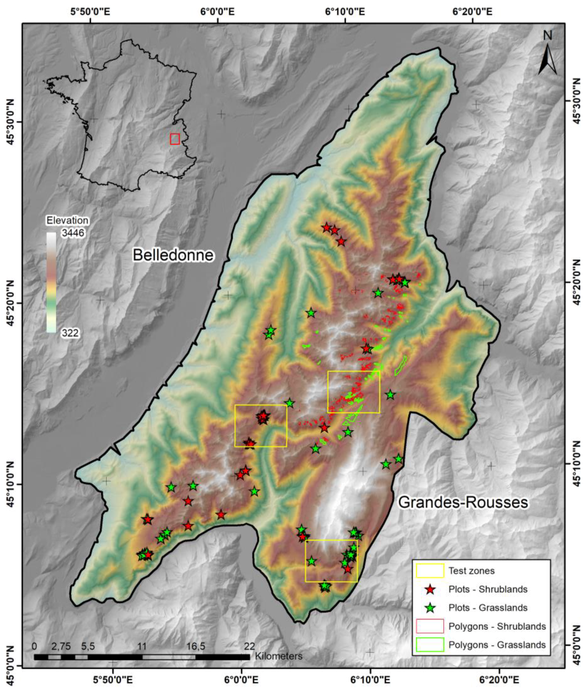
2.1. Study Area

The study area is located in the Belledonne and the Grandes Rousses massifs in the French Alps (Figure 1). The elevation gradient ranges from 250 m above sea level (a.s.l.) at the valley floor to 3442 m a.s.l. The surface area is 1377 km², of which 536 km² is composed of above treeline vegetation (above 1600 m and under 2500 m a.s.l.). The Belledonne and the Grandes Rousses massifs are predominantly made of acidic siliceous rocks and exhibit large areas of Ericaceae-dominated shrublands above the treeline. We identified three test zones along a north–south gradient (Figure 1).

2.2. Remote Sensing Data

Sentinel-2 is an Earth observation mission composed of two identical satellites, Sentinel-2A and Sentinel-2B, respectively launched on 23 June 2015 and 7 March 2017. The 5 day revisit time available since March 2017 was combined with 10, 20, or 60 m spatial resolution of spectral bands. We acquired 84 Sentinel-2A and 39 Sentinel-2B (collectively referred to hereafter as S2) optical images for the T31TGL tile from January 2016 to December 2018 in order to compute NARI and NDVI time series for grasslands and shrublands during a 3 year period (N = 123 scenes). From this collection, 11 images from mid-summer to late fall of 2018 were retained to compute further analyses. The multispectral S2 images are composed of 4 spectral bands (B2: 490 nm, B3: 560 nm, B4: 665 nm, B8: 842 nm) at 10 m spatial resolution and 6 spectral bands at 20 m from the Red Edge (B5: 705 nm, B6: 740 nm, and B7: 783 nm) to the NIR and the SWIR domains (B8a: 865 nm, B11: 1610 nm, B12: 2190 nm). Data were downloaded from the French national THEIA platform (http://www.theialand.fr) at level 2A (i.e., orthorectified product in surface reflectance) with clouds and clouds shadows masks provided at 10 and 20 m spatial resolutions. The clouds, the cloud shadows masks, and the atmospheric correction were performed using MAJA (Multi-sensor Atmospheric Correction and Cloud Screening-Atmospheric and Topographic CORrection, MACCS-ATCOR Joint Algorithm). This algorithm includes a correction of atmospheric effects by combining multi-temporal and multi-spectral criteria to estimate the aerosol optical thickness [37] and also applies a topographic correction to account for changes in illumination caused by slope angle and aspect [38] in order to provide “flat reflectance”. A multi-temporal approach (MAJA) has been preferred to multi-spectral (e.g., Sen2cor), as it outperforms it when highly repetitive observations with constant viewing angles are available [39].

To calculate vegetation indices, five bands were used: three at 10 m resolution (B3, B4, and B8) and two at 20 m resolution (B5 and B11). The 20 m resolution bands were resampled to 10 meters using bilinear interpolation. Bands values were converted from 64 bit signed integer format to reflectance varying from 0 to 1. We also added a constant (0.05) to visible bands B3, B4, and B5 to correct for noise due to surface reflectance correction (comm. pers. O. Hagolle, https://github.com/olivierhagolle). For each atmospheric and terrain corrected image from 2016 to 2018, we calculated (i) the Normalized Anthocyanin Reflectance Index (NARI), which is a normalization of the ARI index presented in Gitelson et al. (2004; ARI = 1/R550 – 1/R700) and is sensitive to plant canopy anthocyanin content; (ii) the Normalized Difference Vegetation Index (NDVI) [40], as it has been widely used for land cover classification (e.g., [41]),. In addition, we estimated the (iii) Normalized Difference Snow Index (NDSI) to identify the presence or the absence of snow cover in a pixel based on a threshold of 0.4 [42]. While this method is known to be inefficient in forested areas [43], it was appropriate to use in our case, as our studied ecosystems are located above treeline. NARI, NDVI, and NDSI were calculated as follows:

$$\left(i\right) NARI=\frac{\left(\frac{1}{Rgreen} - \frac{1}{Rred-edge}\right)}{\left(\frac{1}{Rgreen}+ \frac{1}{Rred-edge}\right)}$$

(1)

$$\left(ii\right) NDVI= \frac{\left(Rnir-Rred\right)}{\left(Rnir+Rred\right)}$$

(2)

$$\left(iii\right) NDSI= \frac{\left(Rgreen-Rswir\right)}{\left(Rgreen+Rswir\right)}$$

(3)

where R is the reflectance of the green (B3), the red (B4), the red-edge (B5), the near-infrared (B8), and the shortwave-infrared (B11) channels. Spectral responses of vegetation communities identified in the field as pure end-member pixels of Ericaceae-dominated shrubland and grassland communities were assessed using a hyperspectral image acquired on 28 September 2015 at the Col de Balme (1950 m a.s.l.) in the nearby Mont-Blanc massif (Project ISOTHERM). The image was acquired using a Fenix hyperspectral camera and consisted of 622 bands ranging from 400 to 2500 nm with an average bandwidth of 30 nm. Raw imagery was processed using the Airborne Processing Library (APL) software and delivered at level 1b (georeferenced and radiometrically corrected).

2.3. Snow, Cloud, and Topographic Masks

For each scene, we applied masks to exclude snow-covered, shadowed, and cloud-covered pixels from our analysis. Cloud masks computed for each date were provided by THEIA. We computed a hillshade mask using a 25 meter digital elevation model [DEM, European Digital Elevation Model (EU-DEM), version 1.0] resampled to 10 m using bilinear interpolation to align with S2 bands. Slope and aspect were computed using the Horn algorithm [44] implemented in R using the terrain function in the raster package [45]. Hillshade was calculated for each scene by combining solar azimuth and elevation (computed as 90 – zenith), which were used as inputs in the hillShade function in the raster package (based on Horn [44]). Mask values ranged from 0 to 1 and represented illumination, with a value of 0 representing complete darkness. Given that poorly illuminated pixels can lead to erroneous reflectance values, we applied a manually calibrated threshold to generate a shadow mask (pixels with an illumination value < 0.25 were excluded). Snow cover maps derived from NDSI (as described above) were used for snow masking.

We calculated seasonal variations in the percentage of snow cover extent, cloud, and shadow masks for all scenes over the three years. A cubic smooth spline (smoothing parameter of 0.4) was fitted to the data in order to estimate the daily change in snow cover extent and cloud cover and to quantify surface loss due to snow and cloud cover over the three years. Pixels of the resulting classification below 1600 m a.s.l. and with NDVI < 0.2 (calculated using 08-28-2018 as a reference) were excluded from the analysis, as they corresponded to below treeline vegetation or sparsely vegetated areas. Finally, water surfaces were also masked using a 10 meter buffer mask.

2.4. Anthocyanin Mapping Protocol

After applying masks, we implemented three approaches to discriminate shrublands from grasslands using NARI. First, we assessed trends in NARI from mid-summer, when anthocyanins levels are expected to be low (hereafter NARI-low date; 19 July 2018), to fall, when anthocyanins levels are expected to be higher (hereafter NARI-high date; 27 September 2018). We utilized a total of six dates and applied a median-based linear model (mblm) using the Theil–Sen single median algorithm [46] fitted between NARI and date for unmasked pixels. A pixel was excluded from the analysis if there were fewer than three available NARI values in the time series. The Theil–Sen procedure is a rank-based test that calculates the non-parametric slope and the intercept of time–series [46]. It is known to be robust for small, heterogeneous datasets containing outliers. We used pixel-level slope coefficients to calibrate a classification threshold for identifying pixels dominated by Ericaceae shrubs, hereafter referred as the “mblm” method. Second, we calculated a difference between NARI-low and NARI-high dates to quantify change in anthocyanin accumulation, hereafter referred as the “delta” method. Third, we directly used the index value of the NARI-high date, hereafter referred as the “Monodate” method. Finally, we applied the same three approaches to time series of NDVI in order to compare the effectiveness of the two indices for detecting shrub cover. Threshold values used for classification were obtained using receiver operating characteristic (ROC) curves presented in the Model Validation section.

2.5. Photo-Interpretation and Ground Reference Data

The six models were evaluated using two independent sources of data. First, ten polygons of each cover type were extracted from the CarHAB mapping program [47]. These polygons were generated using a segmentation approach applied to a high-resolution satellite image and were subsequently validated by field observations of vegetation [48]. Second, we digitized a dataset of 294 polygons using photointerpretation of a high-resolution image (Google, DigitalGlobe) from 10 April 2016 in Google Earth Pro during the anthocyanin peak. This image enabled reliable interpretation of Ericaceae-dominated shrublands due to the leaf reddening caused by anthocyanin production (Figure S1). In total, we analyzed 52 grass and 242 shrub polygons, respectively, representing 269 hectares of grassland with an average patch size of 5 hectares (±9.5 ha) and a mean distance between polygon centroids of 550 m (±516 m) and 234 hectares of Ericaceae-dominated shrubland with an average patch size of 1 hectare (±2.4 ha) and a mean distance between polygon centroids of 137 m (±100 m). As average distance between ground samples was superior to average patch size, we assumed spatial independence between samples. We used 70% of the grassland and the shrubland polygons for model calibration and used the remaining 30% of the dataset for model validation, which represented, on average, 57 hectares of grasslands and 52 hectares of shrubland available for validation.

The second source of independent observations consisted of floristic surveys carried out by the National Alpine Botanical Conservatory (CBNA). The dataset included 347 10 x 10 m community plots containing 451 vascular plant species sampled between 2008 and 2016, half of which were sampled in 2016. Each community plot contained a visual estimate of species cover using Braun-Blanquet [49] classes. (1: less than 1%; 2:1 to 5%; 3:5 to 25%; 4:25 to 50%; 5:50 to 75%; 6: up to 75%). We converted these values to relative abundance using mean cover class percentages. Within sampling plots, an expert botanist identified vascular plants and the relative abundance of each species. We identified 174 plots as shrublands, which were characterized by a relative abundance above 50% of target Ericaceae species Vaccinium myrtillus, Vaccinium vitis-idea, Vaccinium uliginosum microphyllum, and Rhododendron ferrurigeum. We identified 173 plots as grasslands, which contained a relative abundance above 25% of target perennial grass species Nardus stricta and Patzkea paniculata and below 1% of Ericaceae shrubs.

Due to potential signal distortion caused by rock or tree and uncertainties in plot location (Figure S2 shows Google Earth images of two typical cases of distorted signal due to surrounding environmental conditions), the 347 plots were visually verified using very high-resolution images from Google Earth Pro in order to select above treeline plots with homogenous land cover. Furthermore, plots containing more than 5% cover of coniferous tree species Pinus cembra, Pinus mugo, and Picea abies were identified as open forest and were excluded from the analysis. Thus, from the 174 plots initially assigned as shrublands, 80 were in open or closed forest, 36 in screes, and 28 masked by clouds, resulting in 30 plots of homogenous above treeline shrub cover. For the 173 plots assigned as grasslands, 21 were in forests, 23 masked, and 59 in screes, leaving a remaining 70 plots for analysis. For each plot, model values were extracted by averaging values extracted using a 10 m buffer around the plot coordinates. Shrubland plots have a mean elevation of 1861 ± 148 m and are mainly composed of Ericaceae species, which are expected to exhibit late fall reddening and grasses that are common beside shrubs (e.g., Nardus stricta). Grassland plots have a mean elevation of 1921 ± 226 m and mostly include above tree-line perennial graminoids that are commonly associated with shrublands and thus are often confused with shrublands in widely used land cover products (e.g., Nardus stricta or Patzkea paniculata). Results for both groups were compared using the Wilcoxon Signed-Rank test.

2.6. Evaluation of Model Performance

We used ROC curves to test the performance of all six approaches (three for NDVI and three for NARI) using the pROC package in R [50]. ROC curves allowed us to identify the optimal approach with the highest success rate for distinguishing between shrublands and grasslands. The three approaches, described as “mblm”, “Delta”, and “Monodate”, were applied to NARI and NDVI time series and were used as explanatory variables with respect to shrubland and grassland field plots identified above. To identify the best method, we first computed the area under the curve (AUC) and tested for significant differences from 0.5, i.e., randomness, using the Mann–Whitney test and following the process outlined in Manson and Graham [51,52]. Second, we assessed whether or not the sensitivity of ROC curves was statistically different at a given level of specificity corresponding to a 5% chance of committing a commission error (0.95, α = 0.05) using a bootstrap method with 2000 replicates as used in Pepe et al. [53]. Third, as the number of masked pixels varied based on the method used, we compared the surface area loss due to cloud, snow, and shadow masks over the study area and for the six mapping approaches. We then retained the model minimizing surfaces loss and maximizing AUC and sensitivity and applied the optimized threshold to discriminate between shrublands and grasslands.

In order to assess the quality of the produced shrub cover maps, we compared the classification to the remaining 30% of ground reference data. Model performance metrics were calculated using 100 repetitions, during which one pixel was randomly selected within each ground-reference polygon to avoid spatial dependencies. Furthermore, to avoid edge effects, only pixels that completely overlapped polygons were retained. Because polygons with small surfaces (inferior to 0.1 ha) or a Polsby-popper measure [54] too low (inferior to 0.25) did not allow for multiple non-autocorrelated or completely overlapped pixels, 18 polygons were discarded from the quality assessment, leaving a total of 71 pixels per run. For each confusion matrix, we calculated several indices, including (i) Recall, which is the fraction of correctly classified pixels with regard to photo-interpreted polygons, (ii) Precision, which represents the fraction of correctly classified pixels with regard to all pixels classified as such in the image, (iii) Omission error rate, which represents the fraction of pixels incorrectly classified as negative, (iv) Commission error rate, which represents the fraction of pixels wrongly classified as positive, (v) Fscore (also known as F-1 score or F-measure), which is the harmonic mean of Recall and Precision, and (vi) the Kappa coefficient (K), which expresses a relative difference between the total accuracy compared to random accuracy based on an arbitrary threshold value.

(i) Recall = TP / (TP+FN),

(4)

(ii) Precision = TP / (TP+FP),

(5)

(iii) Omission error = FN / (FN+TP)

(6)

(iv) Commission error = FP / (FP+TN)

(7)

(v) Fscore = 2 ∗ ((Precision*Recall) / (Precision+Recall)),

(8)

(vi) Kappa = (TA-RA) / (1-RA),

(9)

where TP is True Positive, FP is False Positive, TN is True Negative, TP is True Positive, TA is Total Accuracy, and RA is Random Accuracy. According to Landis and Koch [55], a Kappa coefficient of 0.6 or more can be considered as acceptable.

2.7. Land Cover Comparisons

Three existing LC products were compared to our classification: (i) two classes of the 100 meter resolution 2018 CORINE Land Cover (CLC) available for Europe [8], transitional woodland-shrub (324) and moors and heathland (322), which we considered to be the equivalent of shrublands in our classification, (ii) the mixed tree-shrub-herbaceous class (100) of the 2015 Global European Space Agency Climate Change Initiative (CCI) Land Cover map at a spatial resolution of 300 m [56], and (iii) the woody moorland (36) class of the 10 meter resolution 2017 Occupation des Sols (OSO) LC map, which is only available for France [9]. In order to determine the relevance of comparison with our mapping results, we evaluated the ability of coarse resolution LC products (CLC and CCI) to detect shrub patches. We first converted our raster classification to polygons, then selected shrub patches with surfaces superior to 1 hectare from our classification, leading to a total of 760 polygons. For each pixel of 100 and 300 m of spatial resolution, we measured the fraction covered by shrub polygons in order to select pixels that were dominantly covered by shrubs at the desired spatial resolution. We defined shrub-dominated pixels as those covered by 75% or more of shrub patches and used these pixels as a basis of comparison with land cover maps (Figure S3 provides further details regarding this analysis). This approach resulted in 905, 4046, and 439,073 shrubland pixels as a basis of comparison with CCI, CLC, and OSO products. Our classification was resampled to coarser spatial resolution for CLC and CCI comparisons (respectively, 100 and 300 m). For OSO, CLC, and CCI, to avoid spatial dependencies, approximately 10% of total pixels were randomly sampled with a distance criterion based on nonaligned systematic sampling (package sp in R, [57,58]). We repeated the process 100 times and produced a confusion matrix and resulting statistical analyses. Because calculating flat pixel-based surface area ignores the effects of topography and surface roughness and leads to major underestimation of features in mountainous areas, we used a triangulated irregular network (TIN) to calculate surface areas accounting for topography.

3. Results

3.1. Spectral Responses

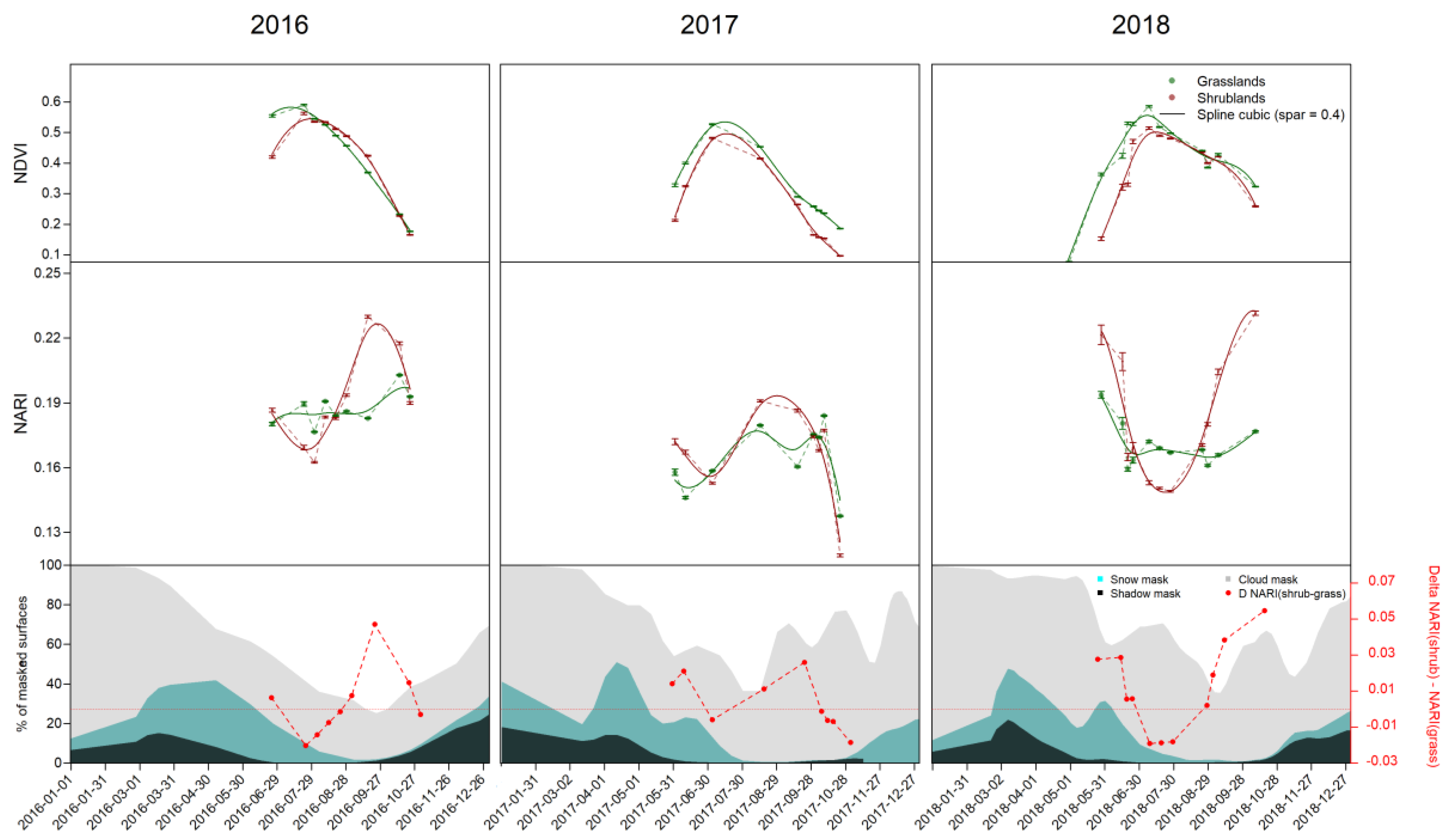
Comparison between end-member pixels corresponding to leaves with and without anthocyanins (respectively dominated by Vaccinium uligonosum and Nardus stricta) demonstrated coherent results with respect to Gittelson et al. [27]. Reflectance in the green band (550 nm) was lower in the case of the shrub canopy, while no substantial difference was observed in the red-edge spectrum (700 nm), suggesting similar chlorophyll content in the two canopies (Figure 2). NARI and NDVI values for the end-members pixels during the late fall yielded similar values to the results presented in Figure 3 (NDVI = 0.46 and 0.44; NARI = 0.18 and 0.25 for N. stricta and V. uliginosum endmembers, respectively).

3.2. Time Series

NDVI dynamics extracted for photo-interpreted polygons of shrublands and grasslands were consistent across the three study years (Figure 3, top panels). Over the course of the growing season, shrublands exhibited slightly lower NDVI values but with similar dynamics compared to grasslands. In contrast, NARI dynamics varied throughout year between grasslands and shrublands (Figure 3, mid panels). In 2016 and 2018, NARI rapidly increased in shrublands starting in early September, peaking in late September and declining between mid to late October. The beginning of the growing season was characterized by high values of NARI for shrublands and slightly lower values for grasslands for the year 2018. Similar trends were not observed for 2016 and 2017 due to high cloud cover leading to pixels obstruction at key dates and an insufficient number of scenes. In contrast to 2016, 2017 and 2018 were characterized by frequent cloud cover during late fall leading to a lack of information (respectively 55% and 60% of surfaces loss at supposed peak due to combined masks for 2017 and 2018, and only 27% for 2016). Nonetheless, for 2018, the supplementary images obtained from Sentinel-2B enabled capturing the late fall reddening of leaves. During the early growing season, high obstruction was observed due to combination of snow and clouds, while obstruction toward the end of the growing season was mostly due to increasing shadows on northern slopes. Four dates with low obstruction from clouds and hillshade were available for 2016 (3 August 2016, 13 August 2016, 23 August 2016, and 22 September 2016). Despite available Sentinel-2B images for 2018, only six dates were cloud-free enough to compute analysis (19 July 2018, 29 July 2018, 28 August 2018, 2 September 2018, 12 September 2018, and 27 September 2018).

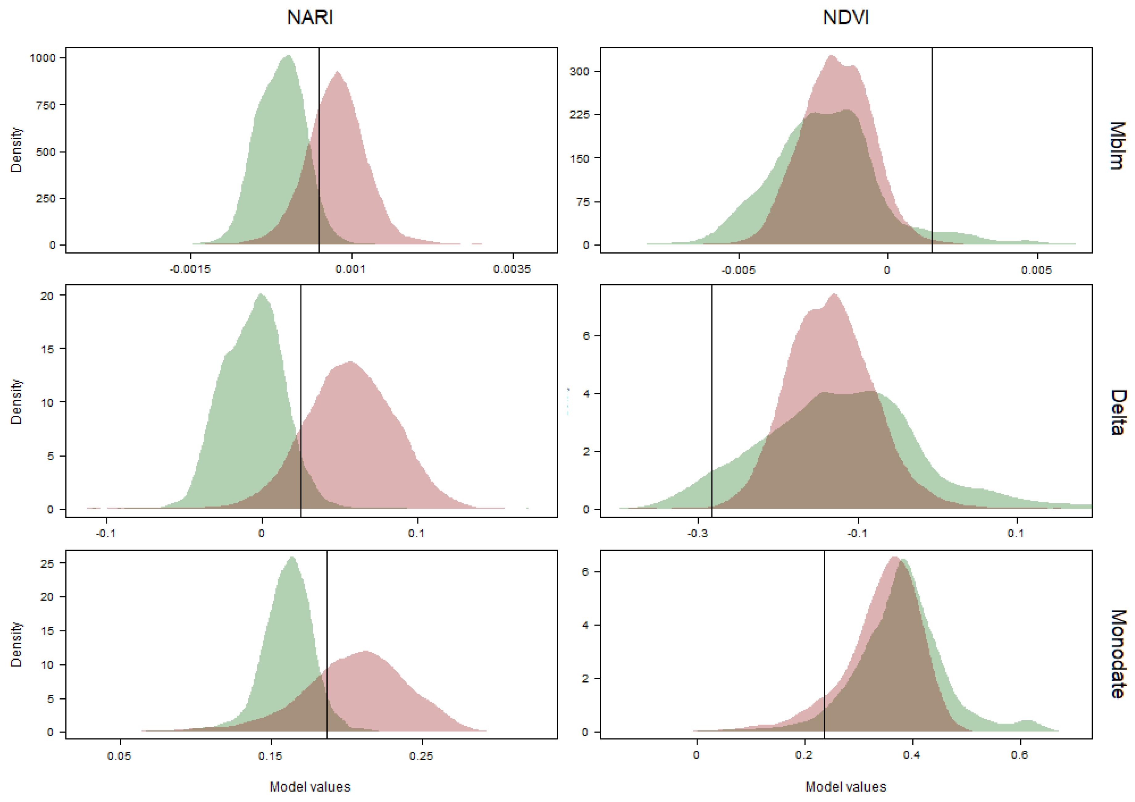
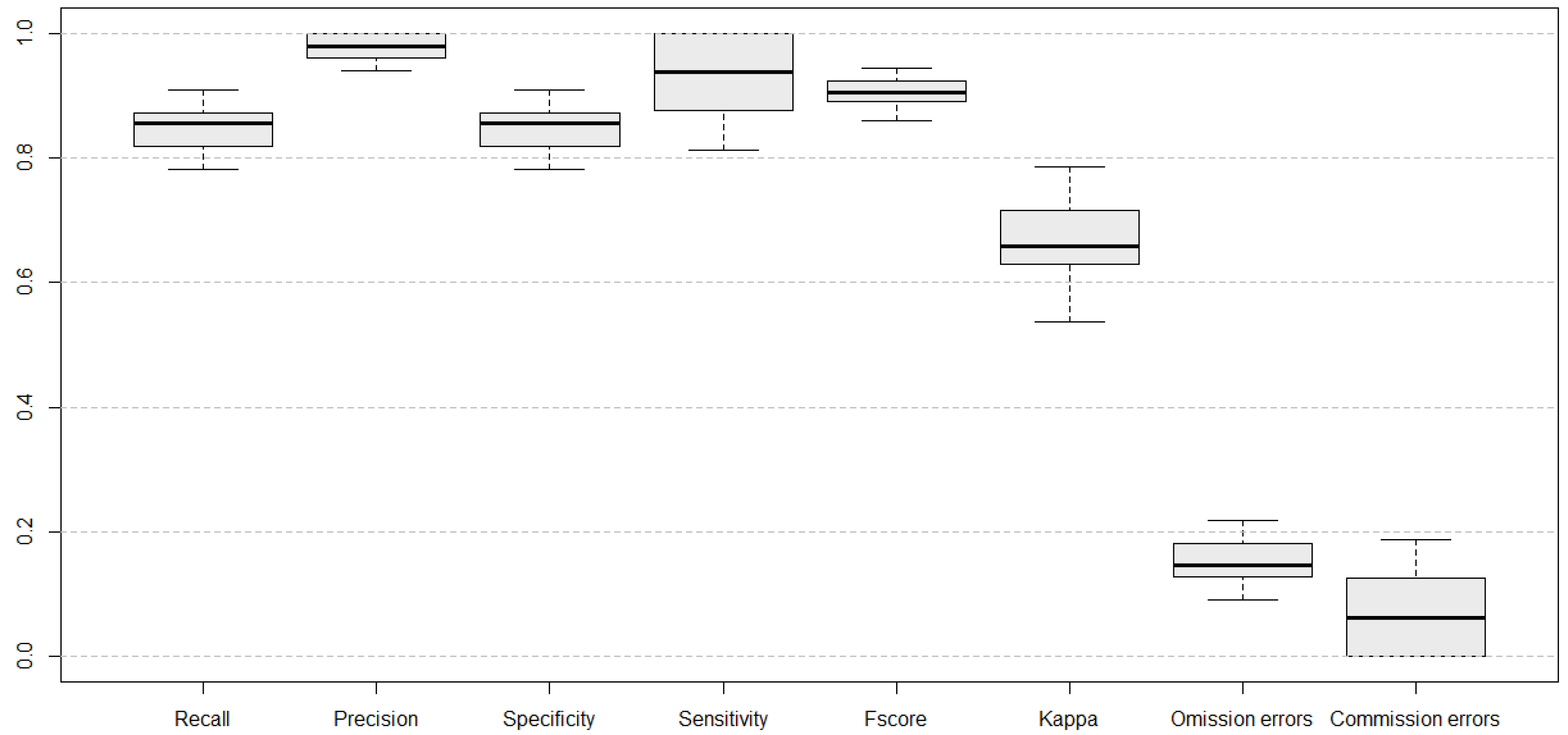
3.3. Best Model and Classification Validation

NDVI-based models showed low AUC (0.61 ± 0.01 on average) and were not significantly different from a random model (Probability-value > 0.05;

Table 1. Statistical results from the six models comparisons, including: area under the curve (AUC) presented with 95% confidence intervals, P-value correspondence (***: <0.001; NS: not significant), the identified statistically optimal threshold, the sensitivity (with specificity fixed as 0.95, α = 0.05) for the selected threshold, and the percentage of masked pixels in the final land cover (LC) map.

			95% CI				Threshold (α = 0.05)
	Models	AUC	-	+	P	Threshold (α = 0.05)	Sensitivity	Masked Pixels (%)
NARI	Monodate	0.87	0.86	0.87	***	0.1869	0.72	14.66
	Delta	0.96	0.96	0.96	***	0.0247	0.86	19.44
	Mblm	0.92	0.92	0.92	***	0.0004	0.72	8.35
NDVI	Monodate	0.61	0.61	0.62	NS	0.2373	0.09	14.66
	Delta	0.54	0.53	0.55	NS	-0.2831	0.00	19.44
	Mblm	0.58	0.57	0.59	NS	0.0014	0.00	8.35

). Also, sensitivity was close to zero for Delta and mblm NDVI models and was 0.23 for the Monodate approach. By contrast, NARI-based models show high AUC (0.92 ± 0.01 on average) with significant difference from a random model (P-val < 1e16), meaning that NARI-based models are more efficient to discriminate shrublands and grasslands (Figure 4). The NARI-based Delta model showed the best results with an AUC of 0.98 and a sensitivity of 0.93, but because this method used only two dates out of the six available, it showed 19.44% of surface loss due to cloud and hillshade. Conversely, the NARI-based mblm model showed low surface loss of 8.35% because the model was calibrated using up to six dates, depending on local cloud cover (Table 1). The remaining surface loss was mainly due to shadows on northern slopes. No significant differences were found between Delta and mblm NARI-based models. Accordingly, the NARI-based mblm model was retained with an optimal classification threshold of 0.0004, i.e., pixels with slope values superior to the threshold were classified as shrublands.

For the NARI mblm model, pixels with values above the optimal threshold were classified as shrublands, and the rest were classified as grasslands. Based on confusion matrices calculated using the 30% remaining polygons of the ground reference dataset (

Table 2. Confusion matrix between NARI-based classification using mblm model and the remaining ground reference data of shrublands and grasslands used for model validation.

Classified as	Shrublands (1)	Grasslands (0)	Total
Shrublands (1)	46.44 ± 1.78 (TP)	1.01 ± 0.84 (FP)	47.45
Grasslands (0)	8.56 ± 1.78 (FN)	14.99 ± 0.84 (TN)	23.55
Total	55	16	71
Omission errors	0.15 ± 0.03
Kappa coefficients	0.67 ± 0.05

), we obtained excellent classification results (Figure 5). The Fscore was 0.90 ± 0.02 with a recall of 0.84 ± 0.03 and a precision of 0.97 ± 0.02, which denotes very low misclassification. Sensitivity and specificity were both high (0.93 ± 0.05 and 0.84 ± 0.03, respectively), indicating a low number of commission and omission errors (respectively, 0.15 ± 0.03 and 0.06 ± 0.05), which means that our classifier was missing approximatively 15% of the shrublands in our study site and was misclassifying approximatively 6% of the grasslands. The Kappa coefficient was 0.67 ± 0.05, which denotes a good classification rate according to Landis and Koch (1977).

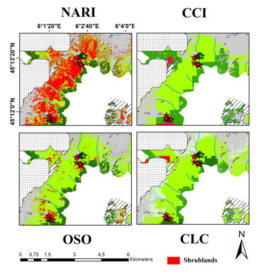
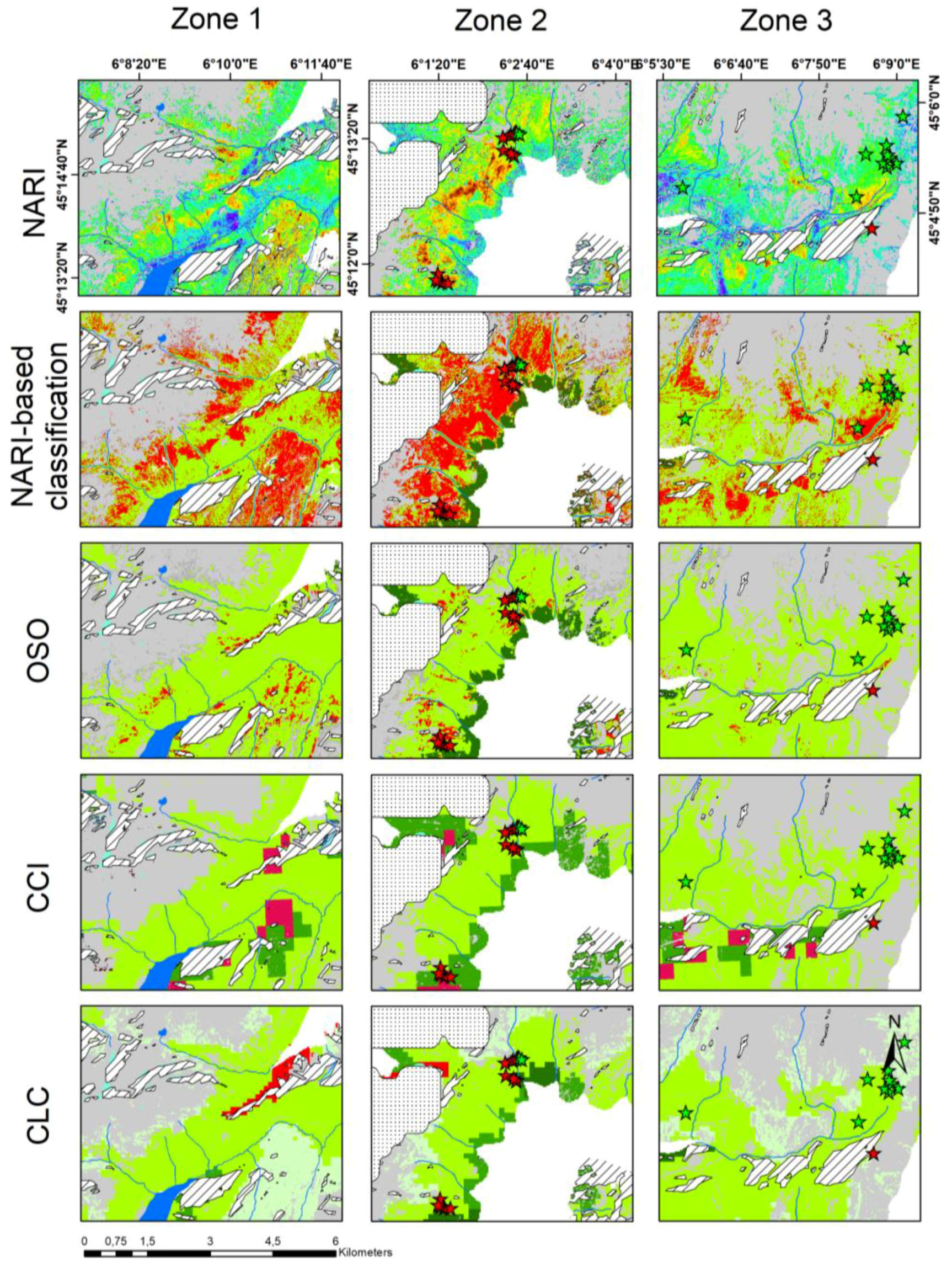
3.4. Comparison with Existing Land Cover Products

Statistical metrics calculated between NARI-based classification and available LC products showed very high omission errors rate of shrublands (

Table 3. Confusion matrices between NARI-based classification and shrublands classes of three widely-use land cover [Occupation des Sols (OSO), Corinne Land Cover (CLC), and CCI in row] in number of pixels. Omission errors and Kappa coefficients are indicated below each corresponding table.

Confusion Matrix OSO
Classified as	Shrublands (1)	Non-shrublands (0)	Total
Shrublands (1)	9414 ± 64	79,646 ± 203	89,060
Non-shrublands (0)	34,501 ± 111	1,119,492 ± 206	1,153,993
Total	43,915	1,199,138	1,243,053
Omission error	0.15 ± 0.03
Kappa coefficient	0.09 ± 0.0009
Confusion matrix CLC
Classified as	Shrublands (1)	Non-shrublands (0)	Total
Shrublands (1)	15.82 ± 2.85	172.72 ± 9.88	189
Non-shrublands (0)	389.03 ± 9.72	11,829.15 ± 16.54	12,218
Total	405	12002	12,407
Omission error	0.96 ± 0.006
Kappa coefficient	0.03 ± 0.009
Confusion matrix CCI
Classified as	Shrublands (1)	Non-shrublands (0)	Total
Shrublands (1)	1.32 ± 1.05	5.08 ± 1.8	6
Non-shrublands (0)	78.71 ± 6.02	1297 ± 6.79	1376
Total	80	1302	1382
Omission error	0.98 ± 0.12
Kappa coefficient	0.02 ± 0.02

). For OSO, CCI, and CLC, the precision was 0.10 ± 0.0006, 0.08 ± 0.01, and 0.20 ± 0.15, respectively, which shows that, on average, 88% of the pixels assigned as shrubland (of adequate size) were misclassified. The omission error rates were 0.78 ± 0.001, 0.96 ± 0.006, and 0.98 ± 0.12, which means that, on average, available LC products misclassified 90% of the shrublands that they were expected to detect in mountainous areas. The Kappa coefficients were 0.09 ± 0.0009, 0.03 ± 0.009, and 0.02 ± 0.02 for OSO, CLC, and CCI, respectively, which denotes a poor classification rate. Given that our omission error rate of our classification was 15%, the estimated surface area of shrublands in our study site was approximatively 102.35 ± 2.67 km², which was approximately 10 times more than shrubland area estimated by existing LC products. Shrublands that were misclassified in available LC products were primarily confused with grasslands (76, 54, and 55% for OSO, CCI, and CLC, respectively) or sparsely vegetated area (22%) for CLC and open coniferous forest (23%) for CCI. Examples of shrubland mapping from NARI-based classification and LC products used for comparison for three test zones show clear underestimation of shrublands surfaces in widely use LC products (Figure 6).

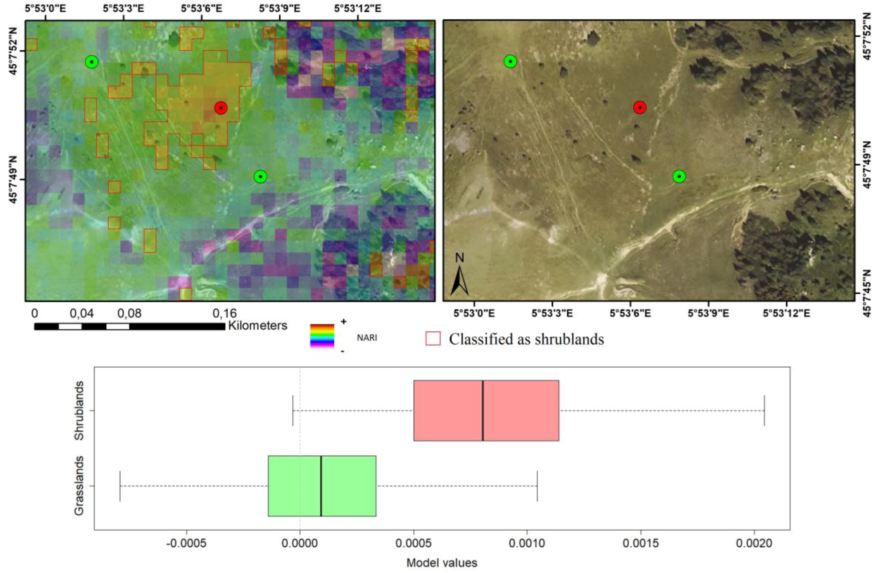
3.5. Validation Relative to Floristic Plots

NARI slope values extracted for 30 shrublands and 70 grasslands of the floristic survey were significantly different (Figure 7; P-val < 2.2e-16). The upper panels of Figure 7 show clear examples of discrimination between shrubland (red) and grassland (green) using NARI slopes values.

4. Discussion

Mapping above treeline shrublands in the Alps using multi-spectral satellite imagery represents a long standing and important challenge [9], given that shrublands represent a substantial portion of above treeline land cover, and shrub encroachment dynamics are of concern for land and conservation managers. Our study used an innovative method to differentiate Ericaceae-dominated shrublands from grasslands, thus enabling improved mapping of shrub cover in mountainous areas. We validated our approach using two independent sources of data, including photo-interpreted polygons produced using very high resolution late fall images and ground-level floristic survey data. In addition to highlighting the utility of the Sentinel-2 red-edge band as well as the importance of high spatial and temporal resolutions, we largely enhanced the detection of shrublands in our study area by demonstrating a 10-fold increase in estimated shrub cover compared to existing LC products.

4.1. Method Caveats and Perspectives

Our method relies on the sensors’ capacity to detect the sharp change in leaf reflectance around 700 nm (red-edge) [59]. It is a key wavelength range sensitive to vegetation conditions and has proven to be useful for quantitative assessment of vegetation properties [60], such as Leaf Area Index (LAI) [61,62,63], chlorophyll or nitrogen content [61,64], chlorophyll-a absorption in turbid and productive waters [65], mapping crop types [66], burn severity [67], and LC mapping [9,68,69,70,71]. Our work represents a novel application aimed at quantifying anthocyanin content in above treeline plant canopies. Given that reciprocal reflectance in the red-edge is only sensitive to chlorophyll and reciprocal reflectance in green is sensitive to anthocyanin, a combination of both bands allows for assessment of pigment concentration [28]. Nonetheless, the formula is only viable because reflectance at 550 nm is almost equal to that at 700 nm in leaves with minute quantities of anthocyanins [72]. Thus, the capacity to detect high relative content of anthocyanin is highly dependent on the central wavelength of the band and te hbandwidth. In Gitelson et al. [28], ARI is developed using bands with red-edge central wavelength at 700 ± 7.5 nm. Because the red-edge Sentinel-2 band is wider (approximately 705 ± 15 nm), noise in the response can be expected. Band 4 (665 ± 15 nm) and band 6 (740 ± 7.5 nm) of S2 have shown no capacity to detect anthocyanin accumulation and thus replace band 5. Thus, the sensitivity of mapping results to bandwidth should be further investigated using hyperspectral data to refine shrubland detection.

Classification of shrublands as one entity suggests that each contributing species exhibits similar responses. Because various levels of reddening are observed between most contributing species (e.g., Vaccinium spp. and Rhododendron ferrugineum), and red-edge position (REP) [73] varies between species due to differences in chlorophyll concentration or biomass [74,75], different phenomena are measured by the Sentinel-2 red-edge band, and various canopy contributions can be expected. In our work, species-level contributions were not investigated due to the constraints of working at the canopy level with multi-spectral satellite imagery. Further analysis of species-level contributions to spectral signatures at the canopy level while accounting for variability over the course of the growing season will require complementary measurements using a field spectrometer [76]. Furthermore, identifying target end members using a field spectrometer would enable sub-pixel fractional mapping of shrub, grasslands, and rocky habitat mosaics, which are ubiquitous features of alpine landscapes.

Among the various tools available for land cover mapping [77], multi-temporal and high-resolution satellite platforms such as Sentinel-2 have been shown to be highly effective [9] due to added information on vegetation phenology [78,79,80]. While seasonal changes in NDVI have already been integrated into land cover mapping protocols [9,81], accounting for seasonal dynamics of plants pigments, such as anthocyanins, represents a novel approach for enhancing high-resolution land cover maps in mountainous areas. Here, we took advantage of the unique dynamics of anthocyanin accumulation in the late fall leaves of shrublands using a multi-temporal approach, demonstrating the potential of classification algorithms using pixel-level trends in seasonal plant pigments (chlorophylls, carotenoids, and anthocyanins) [30]. Alternatively, this unique red pigment activity can be utilized for mapping using a single, very high spatial resolution image acquired at the appropriate season; however, this approach is more difficult to automate, as the timing of peak pigment accumulation varies from year to year.

4.2. Quantifying Shrub Dynamics

The encroachment of shrublands into grasslands in the Alps [17] appears to result from the interaction of multiple factors, including land-use [12,13] and climate change [82,83]. At the local scale, shrub encroachment into species-rich subalpine grassland leads to reduced biodiversity [84,85,86] and diminished pastoral resources [19]. Accordingly, the ability to track shrub dynamics over space and time and understand drivers of shrub expansion is essential to land managers. Compared to currently used LC products, our method allows for improved estimation of the spatial distribution of shrublands at a fine scale and thus moving forward provides decision-makers with a novel tool for land management [87]. Using Sentinel-2, NARI-based shrubland classification can be produced on a yearly basis beginning in 2016, thus allowing for monitoring of shrub dynamics and potential encroachment into grasslands during the coming years.

Understanding the local drivers of shrub expansion, however, necessitates quantifying vegetation dynamics during recent decades. At coarser spatial resolution, MERIS and Sentinel-3 [35] can give continuous NARI time series from 2002 to present, but they are not adapted to complex topographic areas. The Landsat Time Series (LTS), which covers the period from 1984 to present, offers the opportunity to study decadal-scale changes in mountain vegetation [2]. Detecting anthocyanin accumulation within larger 30 m Landsat pixels and with a reduced number of spectral bands represents a significant methodological challenge. A possibility would consist of mapping fractional shrub cover within Landsat pixels, which would require careful calibration with hyperspectral data of end member canopies and as well as calibration of spectral unmixing algorithms across different Landsat satellites. Finally, leaves that concentrate anthocyanins often display characteristics typical of leaves growing under shaded conditions, such as lower chlorophyll a:b ratios [88,89] and higher total chlorophyll content [90,91], which represents a further opportunity.

Quantifying land cover changes requires that observed changes in radiance are resulting from changes in LC and not from variations in atmospheric conditions, soil moisture, sun-surface-sensor geometry, leaf pigmentation [92], or sensor performance [93]. Our method used to classify pixels as shrublands or non-shrublands is highly dependent on the spectral intensity registered at the sensor, and several non-LC related variables can influence mapping results. We are confident that using high performance algorithms [37] prevents errors related to atmospheric conditions. Nonetheless, we recommend applying the bidirectional reflectance distribution function (BRDF) correction mostly to account for “day of year” effects [94], as “view angle” and “mean local time drift” effects are not expected for Sentinel-2 at this scale. Several methods are available to correct for such effects using Sentinel-2 images [95,96]. Due to the progressive accumulation of anthocyanins during an extended period (approximately two months) and the limited number of available scenes, we expect that date availability will vary from year to year. Nonetheless, we are confident that trend estimation using robust models such as mblm can partly override this issue. Finally, because anthocyanin concentration is related to climate variables [97,98], the timing and the intensity of peak accumulation of anthocyanins are expected to vary between years, leading to changes in resulting land cover maps that would be non-representative of shifts in vegetation. Although quantifying this variability remains to be carried out, our initial recommendation for long-term monitoring is to produce averaged shrub cover maps over five year periods in order to smooth inter-annual variability in climate and pigment dynamics. Finally, because temperature and irradiation vary along gradients of elevation, slope aspect, and latitude [99], substantial spatial variations in reddening intensity are expected for a given species across broad study areas. An efficient methodology for long-term monitoring of shrub dynamics at biogeographic scales will thus need to account for these considerations.

4.3. Perspectives for Shrub Mapping in the Arctic

Circum-Arctic measures of vegetation dynamics by satellites indicate widespread patterns of recent greening [100,101,102,103] associated with warming trends [104]. Greening trends have been partly attributed to increases in shrub cover [13] with various responses depending on shrub species and investigated region [105,106]. In the Eastern Canadian Arctic, greening trends are mostly due to increases in Betula glandulosa cover [13,107], which affect competition between species [108] and soil thermal regimes [109,110]. Climate–vegetation feedbacks in the Arctic have important implications for the global climate system, given that shrub expansion into arctic tundra is hypothesized to have direct effects on rates of permafrost thaw and associated release of methane [111]. In the Scandinavian Arctic, multiple artico-alpine Ericaceae shrubs are present (e.g., Vaccinium uliginosum, Vaccinium vitis-idea, and Empetrum nigrum) and could contribute to observed shrub expansion into tundra. Further testing and calibration would be required to evaluate the sensitivity of NARI-based methods for mapping additional dominant arctic shrub species, such as willows (Salix spp.), green alder (Alnus viridis), and dwarf birch (Betula nana). As in the Alps, systematic mapping of shrub cover in the Arctic is both lacking and necessary in order to upscale field-based observations of shrub dynamics to the landscape scale. We encourage further testing and validation of NARI-based approaches in an arctic context in order to determine if this method could be integrated into existing monitoring schemes carried out in the Arctic [112].

5. Conclusions

This work presents an innovative method for differentiating above-treeline shrublands from grasslands in a temperate alpine context based on the detection of anthocyanins in Ericaceae-dominated plant canopies during the late fall. We propose that our method could form the basis for improved monitoring of mountain shrubland dynamics in the coming years during the ongoing Sentinel-2 mission. We demonstrate the poor capacity of widely used land cover maps to identify shrublands as well as the gain in performance associated with our approach. Further work is necessary to establish a relation between anthocyanin content in leaves and NARI using field measurements of leaf spectroscopy and considering local climate conditions, topographic variables, and species contributions to canopy-level reflectance. An additional challenge consists of tracking shrub dynamics during recent decades using cross-calibration between Sentinel-2 and the Landsat archive.

References

1. Rubel, F.; Brugger, K.; Haslinger, K.; Auer, I. The climate of the European Alps: Shift of very high resolution Köppen-Geiger climate zones 1800–2100. Meteorol. Z. 2017, 26, 115–125. [Google Scholar] [CrossRef]
2. Carlson, B.Z.; Corona, M.C.; Dentant, C.; Bonet, R.; Thuiller, W.; Choler, P. Observed long-term greening of alpine vegetation—A case study in the French Alps. Environ. Res. Lett. 2017, 12, 114006. [Google Scholar] [CrossRef]
3. Lamprecht, A.; Semenchuk, P.R.; Steinbauer, K.; Winkler, M.; Pauli, H. Climate change leads to accelerated transformation of high-elevation vegetation in the central Alps. New Phytol. 2018, 220, 447–459. [Google Scholar] [CrossRef] [PubMed]
4. Running, S.W. Ecosystem Disturbance, Carbon, and Climate. Science 2008, 321, 652–653. [Google Scholar] [CrossRef] [PubMed]
5. Zell, E.; Huff, A.K.; Carpenter, A.T.; Friedl, L.A. A user-driven approach to determining critical earth observation priorities for societal benefit. IEEE J. Sel. Top. Appl. Earth Obs. Remote Sens. 2012, 5, 1594–1602. [Google Scholar] [CrossRef]
6. Sterling, S.M.; Ducharne, A.; Polcher, J. The impact of global land-cover change on the terrestrial water cycle. Nat. Clim. Chang. 2012, 3, 385–390. [Google Scholar] [CrossRef]
7. Hansen, M.C.; Potapov, V.P.; Moore, R.; Hancher, M.; Turubanova, S.A.; Tyukavina, A.; Thau, D.; Stehman, V.S.; Goetz, S.J.; Loveland, T.R.; et al. High-resolution global maps of 21st-century forest cover change. Science 2013, 342, 850–853. [Google Scholar] [CrossRef]
8. Bossard, M.; Feranec, J.; Otahel, J. CORINE Land Cover Technical Guide—Addendum 2000; Europen Environment Agency: Copenhagen, Denmark, 2000. [Google Scholar]
9. Inglada, J.; Vincent, A.; Arias, M.; Tardy, B.; Morin, D.; Rodes, I. Operational high resolution land cover map production at the country scale using satellite image time series. Remote Sens. 2017, 9, 95. [Google Scholar] [CrossRef]
10. Jiang, H.; Wang, S.; Cao, X.; Yang, C.; Zhang, Z.; Wang, X. A shadow-eliminated vegetation index (SEVI) for removal of self and cast shadow effects on vegetation in rugged terrains. Int. J. Dig.Earth 2018, 12, 1013–1029. [Google Scholar] [CrossRef]
11. Elmendorf, S.C.; Henry, G.H.; Hollister, R.D.; Bjork, R.G.; Bjorkman, A.D.; Callaghan, T.V.; Collier, L.S.; Cooper, E.J.; Cornelissen, J.H.; Day, T.A.; et al. Global assessment of experimental climate warming on tundra vegetation: Heterogeneity over space and time. Ecol. Lett. 2012, 15, 164–175. [Google Scholar] [CrossRef]
12. Motta, R.; Nola, P. Growth trends and dynamics in sub-alpine forest stands in the Varaita Valley (Piedmont, Italy) and their relationships with human activities and global change. J. Veg. Sci. 2001, 12, 219–230. [Google Scholar] [CrossRef]
13. Myers-Smith, I.H.; Forbes, B.C.; Wilmking, M.; Hallinger, M.; Lantz, T.; Blok, D.; Tape, K.D.; Macias-Fauria, M.; Sass-Klaassen, U.; Lévesque, E.; et al. Shrub expansion in tundra ecosystems: Dynamics, impacts and research priorities. Environ. Res. Lett. 2011, 6, 045509. [Google Scholar] [CrossRef]
14. MacDonald, D.; Crabtree, J.R.; Wiesinger, G.; Dax, T.; Stamou, N.; Fleury, P.; Gutierrez Lazpita, J.; Gibon, A. Agricultural abandonment in mountain areas of Europe: Environmental consequences and policy response. J. Environ. Manag. 2000, 59, 47–69. [Google Scholar] [CrossRef]
15. Gehrig-Fasel, J.; Guisan, A.; Zimmermann, N.E. Tree line shifts in the Swiss Alps: Climate change or land abandonment? J. Veg. Sci. 2007, 18, 571–582. [Google Scholar] [CrossRef]
16. Carlson, B.Z.; Renaud, J.; Biron, P.E.; Choler, P. Long-term modeling of the forest–grassland ecotone in the French Alps: Implications for land management and conservation. Ecol. Appl. 2014, 24, 1213–1225. [Google Scholar] [CrossRef]
17. Cannone, N.; Sgorbati, S.; Guglielmin, M. Unexpected impacts of climate change on alpine vegetation. Front. Ecol. Environ. 2007, 5, 360–364. [Google Scholar] [CrossRef]
18. Anthelme, F.; Villaret, J.C.; Brun, J.J. Shrub encroachment in the Alps gives rise to the convergence of sub-alpine communities on a regional scale. J. Veg. Sci. 2007, 18, 355–362. [Google Scholar] [CrossRef]
19. Eldridge, D.J.; Soliveres, S. Are shrubs really a sign of declining ecosystem function? Disentangling the myths and truths of woody encroachment in Australia. Aust. J. Bot. 2015, 62, 594. [Google Scholar] [CrossRef]
20. Coley, P.D.; Aide, T.M. Red coloration of tropical young leaves: A possible antifungal defence? J. Trop. Ecol. 1989, 5, 293–300. [Google Scholar] [CrossRef]
21. Oberbauer, S.F.; Starr, G. The role of anthocyanins for photosynthesis of alaskan arctic evergreens during snowmelt. Adv. Bot. Res. 2002, 37, 129. [Google Scholar] [CrossRef]
22. Grotewold, E. The genetics and biochemistry of floral pigments. Annu. Rev. Plant Biol. 2006, 57, 761–780. [Google Scholar] [CrossRef]
23. Chalker-Scott, L. Environmental significance of anthocyanins in plant stress responses. Photochem. Photobiol. 1999, 70, 1–9. [Google Scholar] [CrossRef]
24. Tattini, M.; Landi, M.; Brunetti, C.; Giordano, C.; Remorini, D.; Gould, K.S.; Guidi, L. Epidermal coumaroyl anthocyanins protect sweet basil against excess light stress: Multiple consequences of light attenuation. Physiol. Plant 2014, 152, 585–598. [Google Scholar] [CrossRef] [PubMed]
25. Hughes, N.M.; Neufeld, H.S.; Burkey, K.O. Functional role of anthocyanins in high-light winter leaves of the evergreen herb Galax urceolata. New Phytol. 2005, 168, 575–587. [Google Scholar] [CrossRef] [PubMed]
26. Hughes, N.M. Winter leaf reddening in ‘evergreen’ species. New Phytol. 2011, 190, 573–581. [Google Scholar] [CrossRef] [PubMed]
27. Mucina, L.; Bültmann, H.; Dierßen, K.; Theurillat, J.P.; Raus, T.; Čarni, A.; Šumberová, K.; Willner, W.; Dengler, J.; García, R.G.; et al. Vegetation of Europe: Hierarchical floristic classification systemof vascular plant, bryophyte, lichen, and algal communities. Appl. Veg. Sci. 2016, 19, 3–264. [Google Scholar] [CrossRef]
28. Gitelson, A.A.; Merzlyak, M.N.; Chivkunova, O.B. Optical properties and nondestructive estimation of anthocyanin content in plant leaves. Photochem. Photobiol. 2001, 74, 38–45. [Google Scholar] [CrossRef]
29. Gitelson, A.A.; Merzlyak, M.N. Non-destructive assessment of chlorophyll carotenoid and anthocyanin content in higher plant leaves: Principles and algorithms. Remote Sens. Agric. Environ. 2004, 263, 78–94. [Google Scholar]
30. Gitelson, A.A.; Keydan, G.P.; Merzlyak, M.N. Three-band model for noninvasive estimation of chlorophyll, carotenoids, and anthocyanin contents in higher plant leaves. Geophys. Res. Lett. 2006, 33, L11402. [Google Scholar] [CrossRef]
31. Steele, M.R.; Gitelson, A.A.; Rundquist, D.C.; Merzlyak, M.N. Nondestructive estimation of anthocyanin content in grapevine leaves. Am. J. Enol. Vitic. 2009, 60, 87–92. [Google Scholar]
32. Vina, A.; Gitelson, A.A. Sensitivity to Foliar Anthocyanin Content of Vegetation Indices Using Green Reflectance. IEEE Geosci. Remote Sens. Lett. 2011, 8, 464–468. [Google Scholar] [CrossRef]
33. Gitelson, A.; Solovchenko, A. Generic Algorithms for Estimating Foliar Pigment Content. Geophys. Res. Lett. 2017, 44, 9293–9298. [Google Scholar] [CrossRef]
34. Gitelson, A.A.; Chivkunova, O.B.; Merzlyak, M.N. Nondestructive estimation of anthocyanins and chlorophylls in anthocyanic leaves. Am. J. Bot. 2009, 96, 1861–1868. [Google Scholar] [CrossRef] [PubMed]
35. Donlon, C.; Berruti, B.; Buongiorno, A.; Ferreira, M.H.; Féménias, P.; Frerick, J.; Goryl, P.; Klein, U.; Laur, H.; Mavrocordatos, C.; et al. The Global Monitoring for Environment and Security (GMES) Sentinel–3 mission. Remote Sens. Environ. 2012, 120, 37–57. [Google Scholar] [CrossRef]
36. Dedieu, J.P.; Carlson, B.; Bigot, S.; Sirguey, P.; Vionnet, V.; Choler, P. On the importance of high-resolution time series of optical imagery for quantifying the effects of snow cover duration on alpine plant habitat. Remote Sens. 2016, 8, 481. [Google Scholar] [CrossRef] [Green Version]
37. Hagolle, O.; Huc, M.; Villa Pascual, D.; Dedieu, G. A multi-temporal and multi-spectral method to estimate aerosol optical thickness over land, for the atmospheric correction of FormoSat-2, LandSat, VENμS and Sentinel-2 images. Remote Sens. 2015, 7, 2668–2691. [Google Scholar] [CrossRef] [Green Version]
38. Dymond, J.R.; Shepherd, J.D. Correction of the topographic effect in remote sensing. IEEE Trans. Geosci. Remote Sens. 1999, 37, 2618–2619. [Google Scholar] [CrossRef]
39. Baetens, L.; Desjardins, C.; Hagolle, O. Validation of Copernicus Sentinel-2 Cloud Masks Obtained from MAJA, Sen2Cor, and FMask Processors Using Reference Cloud Masks Generated with a Supervised Active Learning Procedure. Remote Sens. 2019, 11, 433. [Google Scholar] [CrossRef] [Green Version]
40. Rouse, J.W., Jr.; Haas, R.H.; Schell, J.A.; Deering, D.W. Monitoring Vegetation Systems in the Great Plains with ERTS, NASA SP-351. Third ERTS-1 Symp. 1974, 1, 309–317. [Google Scholar]
41. Defries, R.S.; Townshend, J.R.G. NDVI-derived land cover classifications at a global scale. Int. J. Remote Sens. 2007, 15, 3567–3586. [Google Scholar] [CrossRef]
42. Dozier, J. Spectral signature of alpine snow cover from the Landsat Thematic Mapper. Remote Sens. Environ. 1989, 28, 9–22. [Google Scholar] [CrossRef]
43. Klein, A.G.; Hall, D.K.; Riggs, G.A. Improving snow cover mapping in forests through the use of a canopy reflectance model. Hydrol. Process. 1998, 12, 1723–1744. [Google Scholar] [CrossRef]
44. Horn, B.K.P. Hill shading and the reflectance map. Proc. IEEE 1981, 69, 14–47. [Google Scholar] [CrossRef] [Green Version]
45. Hijmans, R.J. Raster: Geographic Data Analysis and Modeling. R package version 3.0-2. 2019. Available online: https://cran.r-project.org/web/packages/raster/index.html (accessed on 10 November 2019).
46. Sen, P.K. Estimates of the regression coefficient based on Kendall’s Tau. J. Am. Stat. Assoc. 1968, 63, 1379–1389. [Google Scholar] [CrossRef]
47. Choisnet, G.; Bellenfant, S.; Millet, J.; Catteau, E.; Causse, G. Guide méthodologique de cartographie des habitats (CarHab). Off. Fr. Biodiversité 2019. [Google Scholar]
48. Mikolajczak, A.; Maréchal, D.; Sanz, T.; Isenmann, M.; Thierion, V.; Luque, S. Modelling spatial distributions of alpine vegetation: A graph theory approach to delineate ecologically-consistent species assemblages. Ecol. Inform. 2015, 30, 196–202. [Google Scholar] [CrossRef] [Green Version]
49. Braun-Blanquet, J. Über den deckungswert der arten in den pflanzengesellschaften der ordnung Vaccinio-Piceetalia. Jahresber. Naturforschenden Ges. Graubünden 1946, 80, 1944–1946. [Google Scholar] [CrossRef]
50. Robin, X.; Turck, N.; Hainard, A.; Tiberti, N.; Lisacek, F.; Sanchez, J.C.; Muller, M. pROC: An open-source package for R and S+ to analyze and compare ROC curves. BMC Bioinform. 2011, 12, 77. [Google Scholar] [CrossRef]
51. Mason, S.J.; Graham, N.E. Areas beneath the relative operating characteristics (ROC) and relative operating levels (ROL) curves: Statistical significance and interpretation. Q. J. R. Meteorol.Soc. 2002, 128, 2145–2166. [Google Scholar] [CrossRef]
52. NCAR - Research Applications Laboratory. Verification: Weather Forecast Verification Utilities. R package version 1.42. 2015. Available online: https://CRAN.R-project.org/package=verification (accessed on 10 November 2019).
53. Pepe, M.; Longton, G.; Janes, H. Estimation and comparison of Receiver Operating Characteristic curves. Stata J. 2009, 9, 1–16. [Google Scholar] [CrossRef] [Green Version]
54. Polsby, D.D.; Popper, R.D. The Third Criterion: Compactness as a Procedural Safeguard Against Partisan Gerrymandering. Yale Law Policy Rev. 1991, 9, 301. [Google Scholar] [CrossRef]
55. Landis, J.R.; Koch, G.G. The measurement of observer agreement for categorical data. Biometrics 1977, 33, 159–174. [Google Scholar] [CrossRef] [PubMed] [Green Version]
56. Initiative, E.C.C. Land Cover CCI Product User Guide Version 2.0. 2017. Available online: http://maps.elie.ucl.ac.be/CCI/viewer/download/ESACCI-LC-Ph2-PUGv2_2.0.pdf (accessed on 10 November 2019).
57. Pebesma, E.J.; Bivand, R.S. Classes and methods for spatial data in R. R News 2005, 5, 9–13. [Google Scholar]
58. Bivand, R.S.; Pebesma, E.; Gomez-Rubio, V. Applied Spatial Data Analysis with R, 2nd ed.; Springer: New York, NY, USA, 2013. [Google Scholar]
59. Horler, D.N.H.; Dockray, M.; Barber, J. The red edge of plant leaf reflectance. Int. J. Remote Sens. 1983, 4, 273–288. [Google Scholar] [CrossRef]
60. Frampton, W.J.; Dash, J.; Watmough, G.; Milton, E.J. Evaluating the capabilities of Sentinel-2 for quantitative estimation of biophysical variables in vegetation. ISPRS J. Photogramm. Remote Sens. 2013, 82, 83–92. [Google Scholar] [CrossRef] [Green Version]
61. Delegido, J.; Verrelst, J.; Alonso, L.; Moreno, J. Evaluation of Sentinel-2 red-edge bands for empirical estimation of green LAI and chlorophyll content. Sensors 2011, 11, 7063–7081. [Google Scholar] [CrossRef] [PubMed] [Green Version]
62. Delegido, J.; Verrelst, J.; Meza, C.M.; Rivera, J.P.; Alonso, L.; Moreno, J. A red-edge spectral index for remote sensing estimation of green LAI over agroecosystems. Eur. J. Agron. 2013, 46, 42–52. [Google Scholar] [CrossRef]
63. Herrmann, I.; Pimstein, A.; Karnieli, A.; Cohen, Y.; Alchanatis, V.; Bonfil, D.J. LAI assessment of wheat and potato crops by VENμS and Sentinel-2 bands. Remote Sens. Environ. 2011, 115, 2141–2151. [Google Scholar] [CrossRef]
64. Clevers, J.G.P.W.; Gitelson, A.A. Remote estimation of crop and grass chlorophyll and nitrogen content using red-edge bands on Sentinel-2 and -3. Int. J. Appl. Earth Obs. Geoinf. 2013, 23, 344–351. [Google Scholar] [CrossRef]
65. Vanhellemont, Q.; Ruddick, K. Acolite for Sentinel-2: Aquatic Applications of MSI Imagery. In Proceedings of the Living Planet Symposium, Prague, Czech Republic, 9–13 May 2016; Ouwehand, L., Ed.; ESA Communications: Noordwijk, The Netherlands, 2016; Volume 740, p. 55. [Google Scholar]
66. Immitzer, M.; Vuolo, F.; Atzberger, C. First Experience with Sentinel-2 Data for Crop and Tree Species Classifications in Central Europe. Remote Sens. 2016, 8, 166. [Google Scholar] [CrossRef]
67. Fernández-Manso, A.; Fernández-Manso, O.; Quintano, C. SENTINEL-2A red-edge spectral indices suitability for discriminating burn severity. Int. J. Appl. Earth Obs. Geoinf. 2016, 50, 170–175. [Google Scholar] [CrossRef]
68. Forkuor, G.; Dimobe, K.; Serme, I.; Tondoh, J.E. Landsat-8 vs. Sentinel-2: Examining the added value of sentinel-2′s red-edge bands to land-use and land-cover mapping in Burkina Faso. GISci. Remote Sens. 2017, 55, 331–354. [Google Scholar] [CrossRef]
69. Clerici, N.; Valbuena Calderón, C.A.; Posada, J.M. Fusion of Sentinel-1A and Sentinel-2A data for land cover mapping: A case study in the lower Magdalena region, Colombia. J. Maps 2017, 13, 718–726. [Google Scholar] [CrossRef] [Green Version]
70. Griffiths, P.; Nendel, C.; Hostert, P. Intra-annual reflectance composites from Sentinel-2 and Landsat for national-scale crop and land cover mapping. Remote Sens. Environ. 2019, 220, 135–151. [Google Scholar] [CrossRef]
71. Qiu, S.; He, B.; Yin, C.; Liao, Z. Assessments of Sentinel-2 Vegetation Red-Edge Spectral Bands for Improving Land Cover Classification. ISPRS Int. Arch. Photogramm. Remote Sens. Spat. Inf. Sci. 2017, XLII-2/W7, 871–874. [Google Scholar] [CrossRef] [Green Version]
72. Gitelson, A.A.; Merzlyak, M.N. Signature Analysis of Leaf Reflectance Spectra: Algorithm Development for Remote Sensing of Chlorophyll. J. Plant Physiol. 1996, 148, 494–500. [Google Scholar] [CrossRef]
73. Filella, I.; Penuelas, J. The red edge position and shape as indicators of plant chlorophyll content, biomass and hydric status. Int. J. Remote Sens. 2007, 15, 1459–1470. [Google Scholar] [CrossRef]
74. Baranoski, G.V.G.; Rokne, J.G. A practical approach for estimating the red edge position of plant leaf reflectance. Int. J. Remote Sens. 2007, 26, 503–521. [Google Scholar] [CrossRef]
75. Dawson, T.P.; Curran, P.J. A new technique for interpolating the reflectance red edge position. Int. J. Remote Sens. 1998, 19, 2133–2139. [Google Scholar] [CrossRef]
76. Gamon, J.A.; Somers, B.; Malenovský, Z.; Middleton, E.M.; Rascher, U.; Schaepman, M.E. Assessing Vegetation Function with Imaging Spectroscopy. Surv. Geophys. 2019, 40, 489–513. [Google Scholar] [CrossRef] [Green Version]
77. Xie, Y.; Sha, Z.; Yu, M. Remote sensing imagery in vegetation mapping: A review. J. Plant Ecol. 2008, 1, 9–23. [Google Scholar] [CrossRef]
78. Melaas, E.K.; Friedl, M.A.; Zhu, Z. Detecting interannual variation in deciduous broadleaf forest phenology using Landsat TM/ETM+ data. Remote Sens. Environ. 2013, 132, 176–185. [Google Scholar] [CrossRef]
79. Gómez, C.; White, J.C.; Wulder, M.A. Optical remotely sensed time series data for land cover classification: A review. ISPRS J. Photogramm. Remote Sens. 2016, 116, 55–72. [Google Scholar] [CrossRef] [Green Version]
80. Tuanmu, M.N.; Viña, A.; Bearer, S.; Xu, W.; Ouyang, Z.; Zhang, H.; Liu, J. Mapping understory vegetation using phenological characteristics derived from remotely sensed data. Remote Sens. Environ. 2010, 114, 1833–1844. [Google Scholar] [CrossRef]
81. Yu, L.; Wang, J.; Gong, P. Improving 30 m global land-cover map FROM-GLC with time series MODIS and auxiliary data sets: A segmentation-based approach. Int. J. Remote Sens. 2013, 34, 5851–5867. [Google Scholar] [CrossRef]
82. Huss, M.; Bookhagen, B.; Huggel, C.; Jacobsen, D.; Bradley, R.S.; Clague, J.J.; Vuille, M.; Buytaert, W.; Cayan, D.R.; Greenwood, G.; et al. Toward mountains without permanent snow and ice. Earth Future 2017, 5, 418–435. [Google Scholar] [CrossRef]
83. Formica, A.; Farrer, E.C.; Ashton, I.W.; Suding, K.N. Shrub Expansion Over the Past 62 Years in Rocky Mountain Alpine Tundra: Possible Causes and Consequences. Arct. Antarct. Alp. Res. 2018, 46, 616–631. [Google Scholar] [CrossRef] [Green Version]
84. Koch, B.; Edwards, P.J.; Blanckenhorn, W.U.; Walter, T.; Hofer, G. Shrub Encroachment Affects the Diversity of Plants, Butterflies, and Grasshoppers on Two Swiss Subalpine Pastures. Arct. Antarct. Alp. Res. 2018, 47, 345–357. [Google Scholar] [CrossRef] [Green Version]
85. Maurer, K.; Weyand, A.; Fischer, M.; Stöcklin, J. Old cultural traditions, in addition to land use and topography, are shaping plant diversity of grasslands in the Alps. Biol. Conserv. 2006, 130, 438–446. [Google Scholar] [CrossRef]
86. Laiolo, P.; Dondero, F.; Ciliento, E.; Rolando, A. Consequences of pastoral abandonment for the structure and diversity of the alpine avifauna Blackwell Publishing, Ltd. J. Appl. Ecol. 2004, 41, 294–304. [Google Scholar] [CrossRef]
87. Barbaro, L.; Dutoit, T.; Cozic, P. A six-year experimental restoration of biodiversity by shrub-clearing and grazing in calcareous grasslands of the French Prealps. Biodivers. Conserv. 2001, 10, 119–135. [Google Scholar] [CrossRef]
88. Manetas, Y.; Petropoulou, Y.; Psaras, G.K.; Drinia, A. Exposed red (anthocyanic) leaves of Quercus coccifera display shade characteristics. Func. Plant Biol. 2003, 30, 265. [Google Scholar] [CrossRef]
89. Gould, K.; Davies, K.M.; Winefield, C. Anthocyanins: Biosynthesis, Functions, And Applications; Springer: New York, NY, USA, 2009. [Google Scholar]
90. Cao, K.F. Leaf anatomy and chlorophyll content of 12 woody species in contrasting light conditions in a Bornean heath forest. Can. J. Bot. 2000, 78, 1245–1253. [Google Scholar] [CrossRef]
91. Hughes, N.M.; Vogelmann, T.C.; Smith, W.K. Optical effects of abaxial anthocyanin on absorption of red wavelengths by understorey species: Revisiting the back-scatter hypothesis. J. Exp. Bot. 2008, 59, 3435–3442. [Google Scholar] [CrossRef]
92. Mas, J.F. Monitoring land-cover changes: A comparison of change detection techniques. Int. J. Remote Sens. 1999, 20, 139–152. [Google Scholar] [CrossRef]
93. Wang, D.; Morton, D.; Masek, J.; Wu, A.; Nagol, J.; Xiong, X.; Levy, R.; Vermote, E.; Wolfe, R. Impact of sensor degradation on the MODIS NDVI time series. Remote Sens. Environ. 2012, 119, 55–61. [Google Scholar] [CrossRef] [Green Version]
94. Gao, F.; He, T.; Masek, J.G.; Shuai, Y.; Schaaf, C.B.; Wang, Z. Angular Effects and Correction for Medium Resolution Sensors to Support Crop Monitoring. IEEE J. Sel. Top. Appl. Earth Obs. Remote Sens. 2014, 7, 4480–4489. [Google Scholar] [CrossRef]
95. Franch, B.; Vermote, E.; Skakun, S.; Roger, J.C.; Masek, J.; Ju, J.; Villaescusa-Nadal, J.; Santamaria-Artigas, A. A Method for Landsat and Sentinel 2 (HLS) BRDF Normalization. Remote Sens. 2019, 11, 632. [Google Scholar] [CrossRef] [Green Version]
96. Louis, J.; Debaecker, V.; Pflug, B.; Main-Knorn, M.; Bieniarz, J.; Mueller-Wilm, U.; Cadau, E.; Gascon, F. Sentinel-2 Sen2Cor: L2A Processor for Users. In Proceedings of the Living Planet Symposium 2016, Prague, Czech Republic, 9–13 May 2016. [Google Scholar]
97. Ramirez-Valiente, J.A.; Koehler, K.; Cavender-Bares, J. Climatic origins predict variation in photoprotective leaf pigments in response to drought and low temperatures in live oaks (Quercus series Virentes). Tree Physiol. 2015, 35, 521–534. [Google Scholar] [CrossRef] [Green Version]
98. Hoch, W.A.; Zeldin, E.L.; McCown, B.H. Physiological significance of anthocyanins during autumnal leaf senescence. Tree Physiol. 2001, 21, 1–8. [Google Scholar] [CrossRef] [Green Version]
99. Böhner, J.; Antoni, O. Chapter 8: Land-Surface Parameters Specific to Topo-Climatology. In Developments in Soil Science; Elsevier: Amsterdam, The Netherlands, 2009; Volume 33, p. 216. [Google Scholar]
100. Zhu, Z.; Piao, S.; Myneni, R.B.; Huang, M.; Zeng, Z.; Canadell, J.G.; Ciais, P.; Sitch, S.; Friedlingstein, P.; Arneth, A.; et al. Greening of the Earth and its drivers. Nat. Clim. Chang. 2016, 6, 791–795. [Google Scholar] [CrossRef]
101. Guay, K.C.; Beck, P.S.; Berner, L.T.; Goetz, S.J.; Baccini, A.; Buermann, W. Vegetation productivity patterns at high northern latitudes: A multi-sensor satellite data assessment. Glob. Chang. Biol. 2014, 20, 3147–3158. [Google Scholar] [CrossRef] [PubMed]
102. Huang, M.; Piao, S.; Janssens, I.A.; Zhu, Z.; Wang, T.; Wu, D.; Ciais, P.; Myneni, R.B.; Peaucelle, M.; Peng, S.; et al. Velocity of change in vegetation productivity over northern high latitudes. Nat. Ecol. Evol. 2017, 1, 1649–1654. [Google Scholar] [CrossRef] [PubMed]
103. Myers-Smith, I.; Kerby, J.T.; Phoenix, G.K.; Bjerke, J.W.; Epstein, H.E.; Assmann, J.J.; John, C.; Andreu-Hayles, L.; Angers-Blodin, S.; Beck, P.S.A.; et al. Complexity revealed in the greening of the Arctic. EcoEvoRxiv Preprints 2019. [Google Scholar] [CrossRef] [Green Version]
104. Jia, G.J.; Epstein, H.E.; Walker, D.A. Vegetation greening in the Canadian Arctic related to decadal warming. J. Environ. Monit. 2009, 11, 2231–2238. [Google Scholar] [CrossRef]
105. Bjorkman, A.D.; Garcia Criado, M.; Myers-Smith, I.H.; Ravolainen, V.; Jonsdottir, I.S.; Westergaard, K.B.; Lawler, J.P.; Aronsson, M.; Bennett, B.; Gardfjell, H.; et al. Status and trends in Arctic vegetation: Evidence from experimental warming and long-term monitoring. Ambio 2019, 1–15. [Google Scholar] [CrossRef] [Green Version]
106. Myers-Smith, I.H.; Elmendorf, S.C.; Beck, P.S.A.; Wilmking, M.; Hallinger, M.; Blok, D.; Tape, K.D.; Rayback, S.A.; Macias-Fauria, M.; Forbes, B.C.; et al. Climate sensitivity of shrub growth across the tundra biome. Nat. Clim. Chang. 2015, 5, 887–891. [Google Scholar] [CrossRef]
107. Tremblay, B.; Lévesque, E.; Boudreau, S. Recent expansion of erect shrubs in the Low Arctic: Evidence from Eastern Nunavik. Environ. Res. Lett. 2012, 7, 035501. [Google Scholar] [CrossRef] [Green Version]
108. Shevtsova, A.; Haukioja, E.; Ojala, A. Growth Response of Subarctic Dwarf Shrubs, Empetrum nigrum and Vaccinium vitis-idaea, to Manipulated Environmental Conditions and Species Removal. Oikos 1997, 78, 440–458. [Google Scholar] [CrossRef]
109. Domine, F.; Barrere, M.; Sarrazin, D.; Morin, S.; Arnaud, L. Automatic monitoring of the effective thermal conductivity of snow in a low-Arctic shrub tundra. Cryosphere 2015, 9, 1265–1276. [Google Scholar] [CrossRef] [Green Version]
110. Paradis, M.; Lévesque, E.; Boudreau, S. Greater effect of increasing shrub height on winter versus summer soil temperature. Environ. Res. Lett. 2016, 11, 085005. [Google Scholar] [CrossRef]
111. Sturm, M.; Holmgren, J.; McFadden, J.P.; Liston, G.E.; Chapin, F.S.; Racine, C.H. Snow–Shrub Interactions in Arctic Tundra: A Hypothesis with Climatic Implications. J. Clim. 2001, 14, 336–344. [Google Scholar] [CrossRef] [Green Version]
112. Ims, R.A.; Yoccoz, N.G. Ecosystem-based monitoring in the age of rapid climate change and new technologies. Curr. Opinion Environ. Sustain. 2017, 29, 170–176. [Google Scholar] [CrossRef]
Figure 1. Location of the study area within the French Alps. Photo-interpreted polygons and floristic surveys plots are shown in red and green for shrublands and grasslands.
Remotesensing 11 02807 g001
Figure 2. Reflectance distribution of end-members pixels representing Ericaceae-dominated shrublands (dominated by Vaccinium uligonosum) and grasslands (dominated by Nardus stricta) extracted from a hyperspectral image acquired on 28 September 2015 at the Col de Balme [1950 m at sea level (a.s.l.)] in the nearby Mont-Blanc massif. Sentinel-2A bands B3 and B5 used to calculate Normalized Anthocyanin Reflectance Index (NARI) are indicated by grey rectangles in panel (A). Photo of late fall grasslands dominated by Nardus stricta (B) and late fall Vaccinium uligonosum (C; photo credit: Cédric Dentant).
Remotesensing 11 02807 g002
Figure 3. Normalized Difference Vegetation Index (NDVI) (top), NARI (middle), and masked surfaces (bottom) distribution over the three years for shrublands (red) and grasslands (green). The error bars represent the 99% confidence interval. Percentage of masked surfaces are based on the surfaces of the studied area presented in Figure 1, representing 1377 km².
Remotesensing 11 02807 g003
Figure 4. Kernel density plots for shrublands (red) and grasslands (green) for the three NARI (left) and the three NDVI (right) models. Vertical lines represent the statistically optimal classification threshold.
Remotesensing 11 02807 g004
Figure 5. Statistical metrics used to evaluate the performance of the NARI mblm-based model of shrubland classification. Metrics were calculated 100 times using a randomized 50% selection of the photo-interpreted data retained for validation.
Remotesensing 11 02807 g005
Figure 6. Example LC maps of shrublands for three test zones (columns), representing from top to bottom rows: continuous slope values of the NARI model, Corinne Land Cover (CLC), Global ESA CCI Land Cover (CCI), Occupation des Sols (OSO), and NARI-based classification. Shrublands are represented in red.
Remotesensing 11 02807 g006
Figure 7. Examples of vegetation plots identified as shrubland (red) and grassland (green) juxtaposed (left) or not (right) with NARI slopes values and an aerial photograph. Pixels classified as shrubland are indicated by the red outline. Distribution of NARI slope values for shrubland (red, N=30) and grassland (green, N = 70) vegetation plots.
Remotesensing 11 02807 g007