Framework for 3D Point Cloud Modelling Aimed at Road Sight Distance Estimations

Abstract

Existing roads require periodic evaluation in order to ensure safe transportation. Estimations of the available sight distance (ASD) are fundamental to make sure motorists have sufficient visibility to perform basic driving tasks. Mobile LiDAR Systems (MLS) can provide these evaluations with accurate three-dimensional models of the road and surroundings. Similarly, Geographic Information System (GIS) tools have been employed to obtain ASD. Due to the fact that widespread GIS formats used to store digital surface models handle elevation as an attribute of location, the presented methodology has separated the representation of ground and aboveground elements. The road geometry and surrounding ground are stored in digital terrain models (DTM). Correspondingly, abutting vegetation, manmade structures, road assets and other roadside elements are stored in 3D objects and placed on top of the DTM. Both the DTM and 3D objects are accurately obtained from a denoised and classified LiDAR point cloud. Based on the consideration that roadside utilities and most manmade structures are well-defined geometric elements, some visual obstructions are extracted and/or replaced with 3D objects from online warehouses. Different evaluations carried out with this method highlight the tradeoff between the accuracy of the estimations, performance and geometric complexity as well as the benefits of the individual consideration of road assets.

1. Introduction

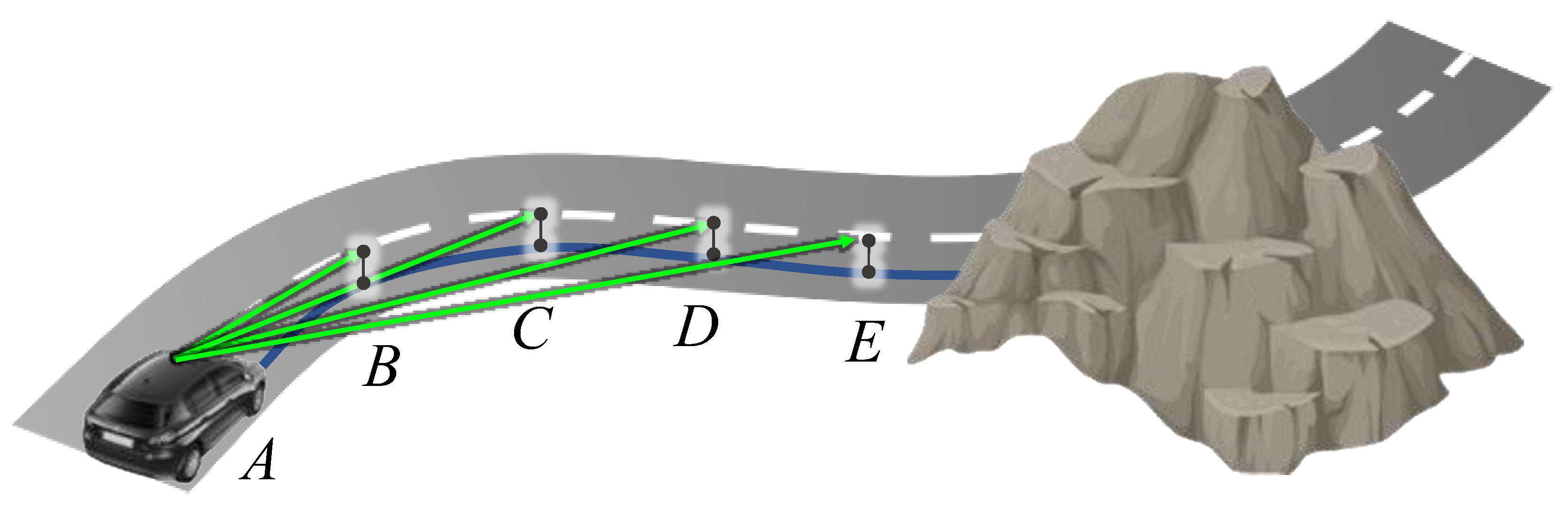
Proper road network operation is ensured by carrying out several asset management, maintenance and safety examinations. In this sense, making sure a road section provides adequate sight distances is fundamental to guarantee its functioning. The available sight distance (ASD) is the length of unobstructed road ahead of drivers. As shown in Figure 1, this distance is measured on the traveled path (blue line). Here, the ASD measured from station A is the curve AE. In order to set common basis that would make results comparisons possible, some road design guidelines indicate the measurement of the ASD along the centerline (to simplify the process) [1], or specify a fixed offset path from the centerline [2].

Motorists collect information concerning road geometry and traffic conditions primarily through their eyesight, then based on that collection, driving decisions are made and maneuvers performed. These maneuvers are conditioned primarily upon horizontal and vertical layout, roadside elements, the road level of service and the ASD, among other factors. Departments of Transportations (DOTs) from different countries define minimum distance values for stopping sight distance (SSD), passing sight distance (PSD), decision sight distance (DSD) and intersection sight distance (ISD) [1,2,3].

The ASD, which depends to a large extent on the geometry of the road and its surroundings, must be checked against the aforementioned required values, as a result, road design guidelines also specify the criteria to measure the ASD. These measurements require the definition of the considered observer eye height and the specification of the placement and height of the object/target. The considered target depends on the sight distance under evaluation, for instance SSD calculations define their target to be an object whereas ISD calculations consider another road user as a target. These factors also have important effects on the resulting ASD. These comparisons are necessary not only during the design stage, where they represent a key factor throughout the alignment process, but also on existing roads. For that reason, visibility and line-of-sight checks are part of road safety audits.

When performing these audits offsite and making use of geospatial data, it is essential to utilize high resolution representations of the road geometry and the elements along the roadside such as road equipment and vegetation. These models ought to be not only realistic and updated enough so as to perform visual inspections, but also must hold sufficient accuracy to perform robust evaluations, measurements and calculations. For these reasons, the use of LiDAR-derived models has been of great use in the field of civil engineering, with applications as wide as the inspection of existing infrastructure [4], road information inventory [5], road safety [6], among others.

Another way of evaluating the ASD on site is through static field measurements or using image-based mobile mapping systems (MMS). These methods are affected by and could affect surrounding traffic. In addition, if the road section is not temporarily closed, static measurements could pose safety risks to technicians on site. Hence the tendency to favor offsite evaluations that employ realistic road models [7]. Current methodologies employ LiDAR data to obtain the needed road representations and assess the ASD offsite. Terrestrial Mobile LiDAR Systems (MLS) are capable of obtaining a 3D sample of the road while covering the desired area at regular speeds. The resulting cloud could be used to perform the evaluations directly in it or could be utilized to obtain a digital model. Another fact stated in the revised literature is the benefit that brings the employment of Geographic Information Systems (GIS) tools to carry out raytracing or visibility functionalities so as to obtain the maximum unobstructed line of sight. GIS also allow the conflation of dissimilar information, the intuitive visualization of results and the evaluation of the 3D alignment coordination [8,9]. When utilizing GIS and traditional vector Digital Surface Models (DSM), so as to evaluate the effect of roadside elements, most obstructions are portrayed as facets in triangulated irregular networks (TIN). However, their elevation is not an independent variable. This misrepresentation becomes a problem when road utilities or foliage overhangs the road and are portrayed as obstructions. As a solution to that problem the authors have proposed a methodology that makes use of 3D objects and traditional terrain models [10]. This way, the terrain can still be represented under traditional 2.5 D elements, hence lowering the computational resources required to be represented, and aboveground elements could be treated separately and even relocated so as to evaluate the impact of their position on visibility.

With these facts into consideration, this research presents a framework for the modeling of 3D objects involved in sight distance estimations while emphasizing the insights of its implementation. The presented methodology solves the problem that arises when traditional Delaunay algorithms are used to obtain the digital models that represent the road environment [11]. The framework considers as main data input a point cloud obtained with MLS. These acquisition platforms allow the extraction of potential obstructions with the required level of detail to perform ASD evaluations. The accuracy of the presented assessments relies, to a great extent, on the quality of the point cloud. As the quality requirements of ASD calculations are high, data was captured following the necessary steps to meet them (additional passes where required, temporal GNSS stations near the survey, required equipment calibration, etc.). The accuracy of the proposed methodology was evaluated in a previous work [12]. ASD values resulting from this method were compared with ASD results obtained by measuring marked targets on photographs. The agreement between these procedures was valuated using the coefficient of agreement κ [13]. Results showed that the overall agreement between the two methods was 0.958.

The remaining of the study is organized as follows: first a description is presented including current methodologies aimed at the evaluation of ASD on existing roads by means of LiDAR data, and their main limitations. Subsequently, the proposed methodology is presented followed by the main results of its implementation on distinct road sections including their main advantages and disadvantages, and finally brief conclusions.

2. Background

Increasing highway speeds and changes in roadside features make road conditions dynamic. These facts stress the need to efficiently ensure sight distance values provided during the design stage. These and other reasons have fostered the proposal of few changes in the way sight distances are calculated and measured. These changes include but are not limited to, the approach, procedures and the models utilized to obtain the ASD. For instance, studies have shown the misestimations that could cause performing these assessments two-dimensionally. When assessed in two dimensions the calculations are performed for distinct elements of horizontal and vertical alignment separately and when these elements are combined the most critical one is chosen. This has been proven to under or overestimate real values and to contribute to not spotting shortcomings in the 3D alignment [14,15]. Visual obstructions could be caused by horizontal or vertical alignment elements or side obstructions. Owing to the benefits of performing these visibility checks with geospatial data, distinct authors have utilized Line of Sight functionalities provided by widespread GIS software [16,17,18]. For this reason other authors have characterized the existing methodologies and procedures to evaluate sight distances as GIS-based and Non-GIS [19].

Concerning the road modeling techniques utilized along the ASD literature, it was found that scientific research whose purpose is the establishment of their proposed frameworks for 3D sight distance analyses in geometric design standards makes great use of parametric idealizations of road sections [14,15,20]. These are focused on modeling the road geometry and leave behind existing structures or vegetation. On the other hand, lines of research aimed at improving ASD estimation procedures on existing roads, show a wide variety of methods for road feature extraction as well as geospatial data acquisition, modeling and processing workflows. Up-to-date models or 3D data of the road and roadside elements are not always available and when available their reliability, temporal validity and timeliness must be checked. For this reason, recent evaluations of sight distances on existing roads have been made by means of LiDAR-derived data. When making use of LiDAR topographical data, some road evaluations are performed directly on the measured cloud [17,21] and others make use of a surface model [22,23]. Performing the evaluations directly on the point cloud consumes less computational resources and does not have the misrepresentation problem that complex geometries could have. However, these methodologies could deliver underestimated values if points which are not an obstruction block the line of sight. On the other hand, the line of sight could pass between adjacent points and provide overestimated values. Newer methodologies have focused on the depiction of complex components of the road scenery proposing modified triangulation algorithms. Ma et al., presented an effective real time method for estimating ASD including a cylindrical perspective projection [19]. Their methodology, however, does not tackle and was not intended to tackle the improvement of road asset positioning. Whether utilizing a model or performed directly on the point cloud, the amount of data used to recreate the road environment should allow accurate measurements while not representing a challenge to the available computational resources.

Moreover, 3D data and 3D approaches have been advantageous to the evaluation of road assets placements as they facilitate the analysis of their impact on safety. Traffic signs, utility poles, concrete barriers, overpasses and other road infrastructure elements as well as street furniture and vegetation have been effectively extracted using MLS. The proposed methodology exposes as an objective the evaluation of the impact of these elements on the ASD and the improvement of their location.

3. Materials and Methods

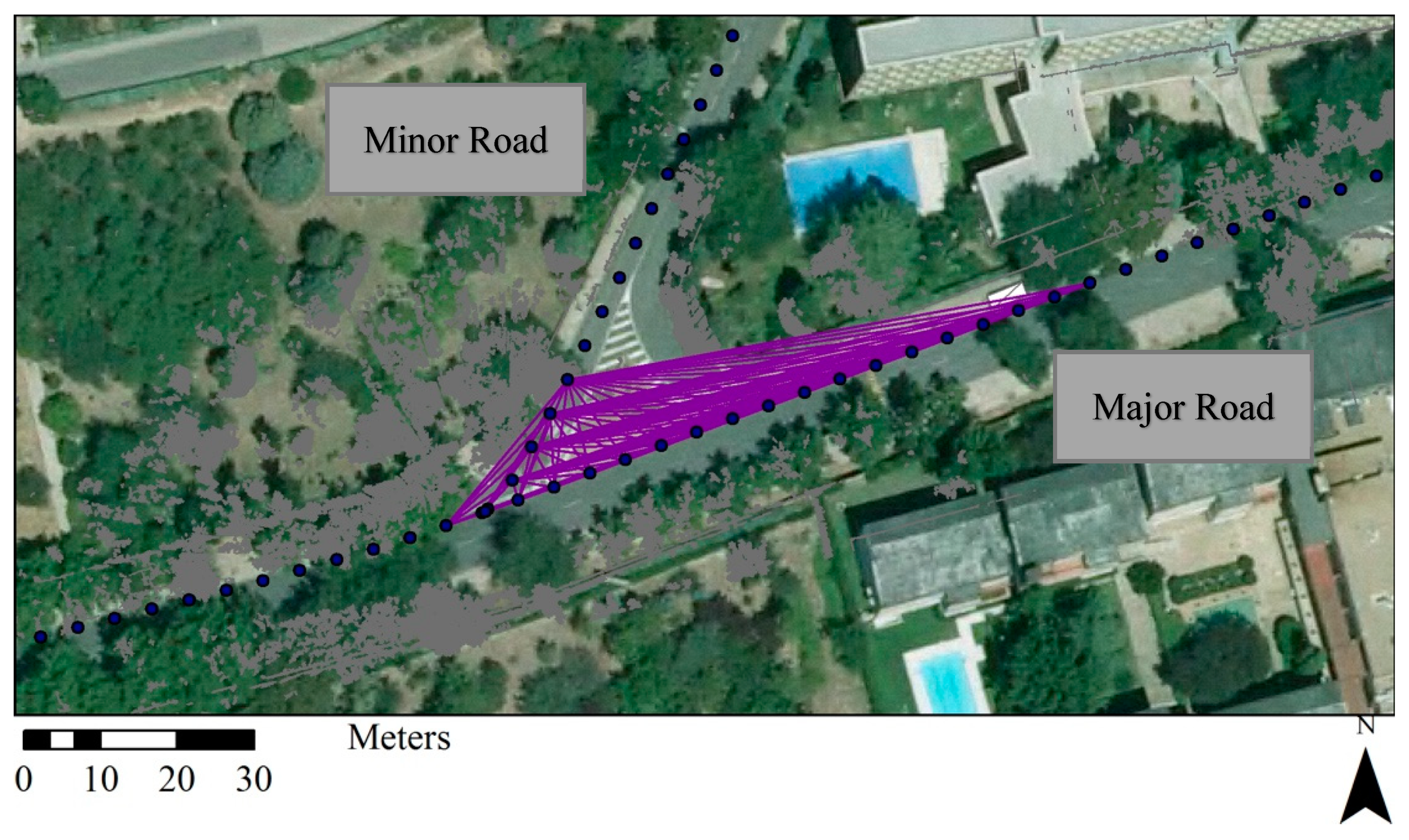
This work describes a methodology devised to obtain ASDs. This GIS-based procedure launches lines-of-sight from the designated observers to the indicated targets. This is done exploiting geospatial functionalities from the ArcGIS software (Esri, Redlands, CA, USA) in its 10.3 version. These and other visibility tools are put together in a validated geoprocessing model [10]. The main tools utilized are: Construct Sight Lines and Line Of Sight. As previously mentioned, these estimations require the definition of a trajectory. This trajectory is discretized into a set of successive and numbered points called stations. These stations represent the positioning of the considered observers and targets. With the targets and objects precisely located, sight lines are built between them (taking into account their height differences). Due to the fact that all points are designated to be both observers and targets a selection of the pertinent lines of sights is made. This selection only considers the visuals launched from the designated initial station and onwards (in ascending order). Subsequently, a layer with these selected lines is created. Finally, the tool Line of Sight is launched with these selected sightlines in order to evaluate their visibility.

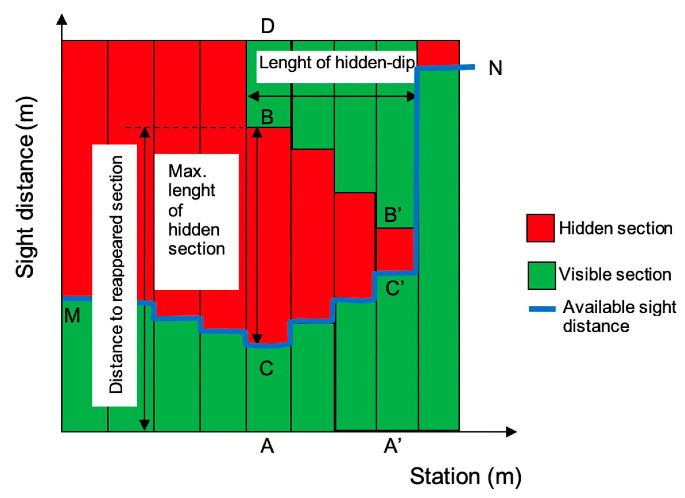
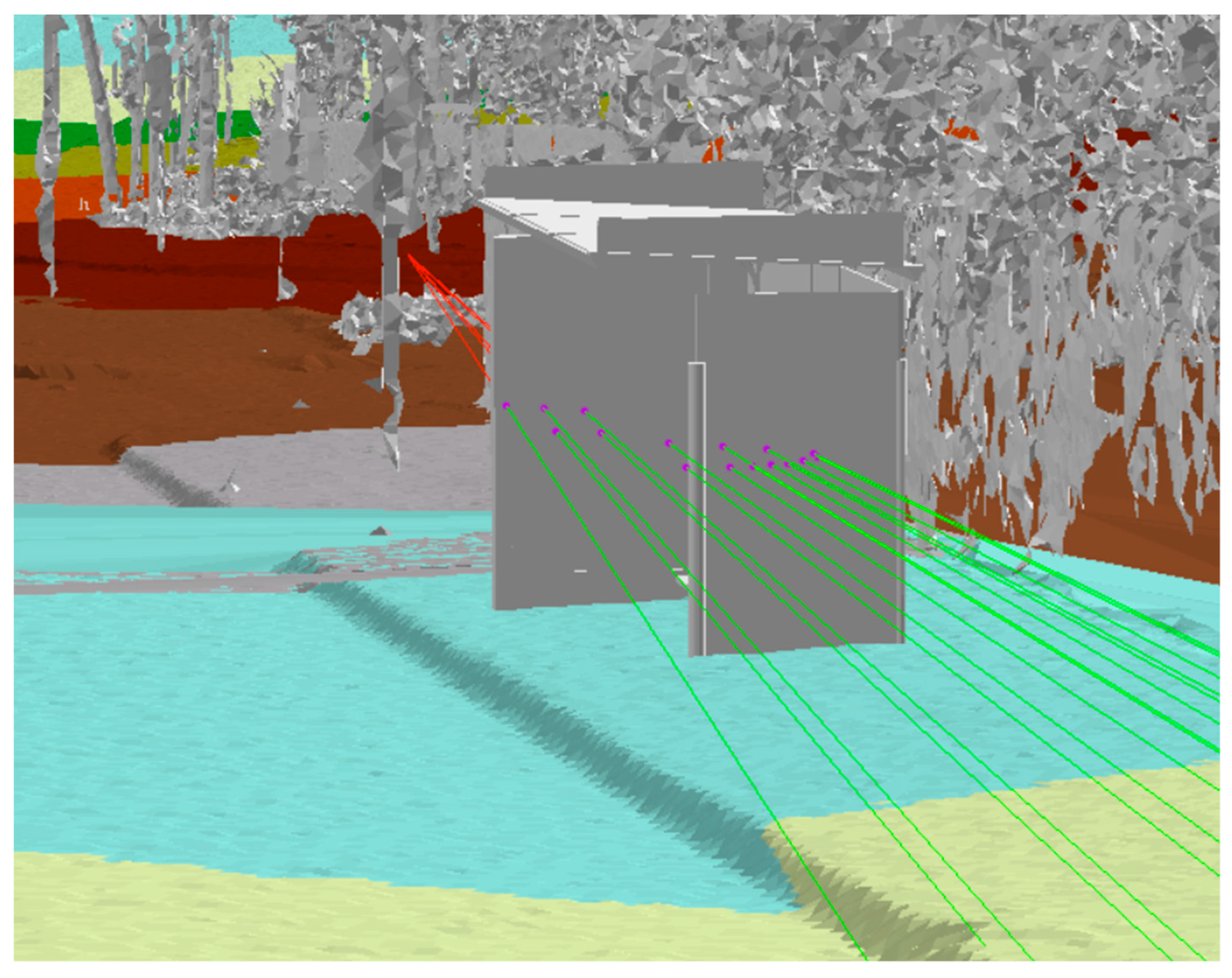
The main results of the methodology are a shapefile of points with the coordinates of the element causing the first obstruction between observer and target, a polyline with the longest unobstructed visual (and the remaining obstructed line), and a sight distance diagram. The points showing the obstructions and the sightlines will be depicted in the following section. The sight diagram is displayed in Figure 2.

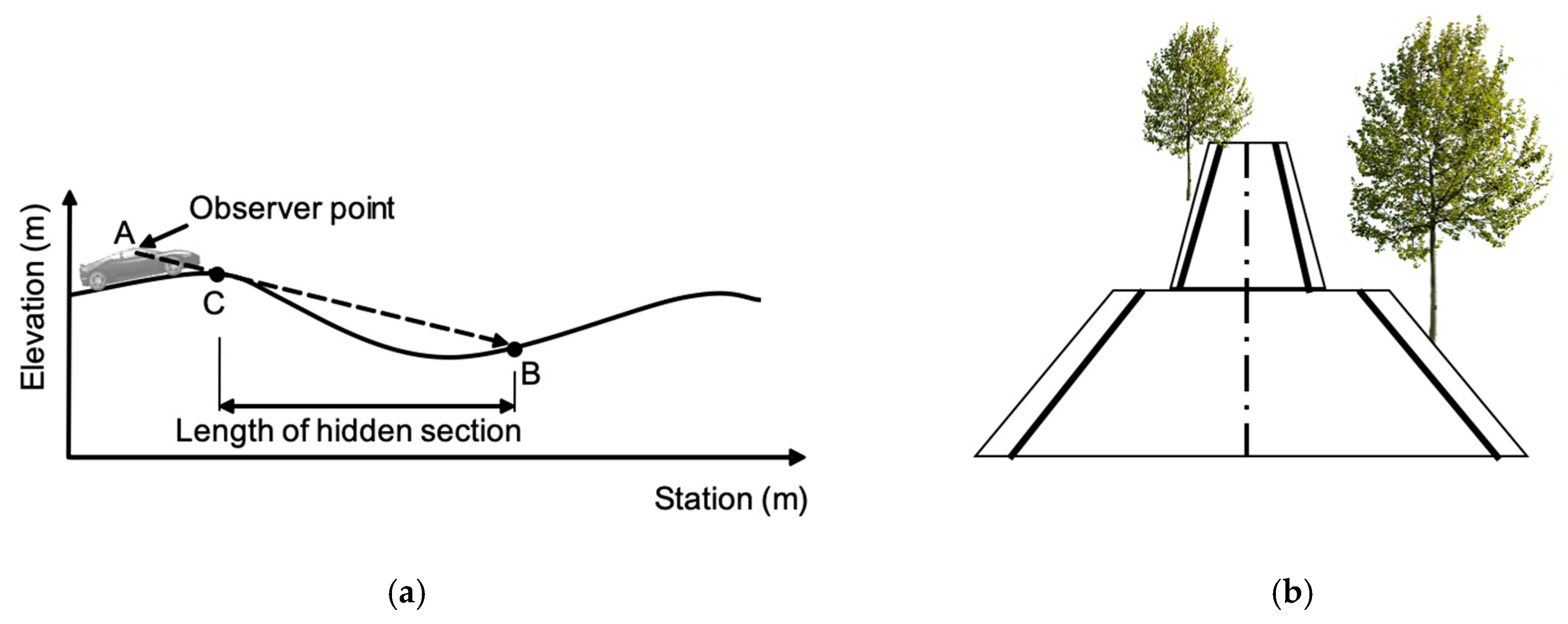
The chart displays the successive stations in the horizontal axis and the sight distances in the vertical one. The green parts show the visible sections and the red ones the non-visible ones. Here, the ASD is represented by the blue line which unites the maximum unobstructed distances among stations. Areas with hidden sections between visible ones are those with hidden dips which could be due to 3D alignment shortcomings. In the diagram, segment MN shows the ASD; AA’ shows the length of the section with a hidden-dip; CB shows the maximum length of the hidden section, which is that segment of the road with the maximum amount of non-visual distances with a visual reappearance; and the distance AB is the total distance, from station A, to the visual reappearance. These partial obstructions in the sight distances are caused by some combination of profile and alignment elements. These are illustrated in Figure 3, the first part (3a) displays the vertical profile (station-elevation chart) showing how two successive crest curves with a sag in between create partial loss in visibility. Figure 3b shows the same alignment disposition from a frontal 3D view.

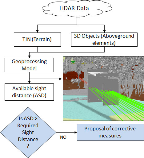
As seen, visual obstructions could be caused by the road geometry itself in addition to the effects of roadside elements (vegetation, crash barriers, roadside topography, elements obstructing horizontal curves clearance, etc.). In this sense, complex 3D objects are represented in GIS utilizing the multipatch format from the ArcGIS software [24]. These could be obtained by importing 3D objects from online libraries or from 3D modeling software. These two, road geometry and roadside features, account for all possible physical visual obstructions. When it comes to the ground, taking advantage of the fact that road geometries depict homogeneous and consistent surfaces, its representation is done utilizing regular TIN models. Terrestrial MMS surveys could deliver clouds whose majority of points belong to the ground, this is due to the fact that the highest density is captured in areas which are closer to the sensors and these are fixed in a car that is traveling along the roadway. Obtaining a proper model from this vast amount of points does not have to consume much representation memory because the limitations of modeling the ground as facets in a TIN do not affect its suitable portrayal.

Figure 4 presents a diagram of the proposed method. As displayed, the evaluation requires a complete description of the road scene and the vehicle trajectory. This trajectory contains both the target and observer’s considered heights. Two important distinctions are made from a classified point cloud. First, those points that belong to the ground are converted to a DTM. When it comes to the aboveground elements a discrimination is made between manmade and natural components. Vegetation, as the main natural element found in road surroundings, is stored in the multipatch file. If foliage comes out as an obstruction of visibility, a suggestion of improving vegetation management is made. Man-made utilities, buildings, furniture and road assets, on the other hand, could be also modeled together in a multipatch file, unless an evaluation of the positioning of a particular element is to be carried out. When the relocation of road assets or street furniture is considered, these elements are analyzed to determine if the level of detail provided by the group of points defining them, is enough to run the evaluation. On the contrary, if the point cloud representation of the element is not dense enough, the element is replaced by another one with its exact dimensions. This element could be modeled or obtained from 3D design software or libraries. This replacing 3D object has to have real measurements. These could be obtained whether measuring the real element, portrayed in the point cloud, or from measurements of the corrected photos acquired with the MMS survey.

As mentioned, this method makes use of a dense and accurate enough point cloud. In this sense, a reasonable density (between 100 and 40 pts/m²) and high network accuracy is strongly suggested in order to obtain reliable results [18]. Below are the processes required to define the models from the LiDAR point cloud. Some of these tasks were also found in road feature extraction and road surface modeling literature [25,26].

3.1. Georreferencing and Denoising

Depending on how processed the point cloud is at the time of acquisition some processing steps might be needed or not. With particular attention to the Coordinate Reference System (CSR), MMS delivered point clouds include the spatial reference information provided by their Global Navigation Satellite System (GNSS) and their Inertial Navigation System (INS). Most pre-processing software deliver data in an appropriate CRS considering the project’s location. Nonetheless, it is common to acquire point clouds that are not referred to the desired system and require transformation or projection processes to be done. This correct referencing is not only important due to its impact on the results but also because it enables the addition of reference or auxiliary spatial information.

Point clouds usually contain noticeable abnormal measurements for specific regions, or gaps in the laser coverage, as a result of inaccurate observations, incorrect returns, register of unwanted features, obstruction of the LiDAR pulse, instrument or processing anomalies among other possible causes. These artifacts ought to be removed from the point cloud. For MMS derived data, it is common to require the removal of traffic around the surveying vehicle. These points ought to be deleted so as to enable the obtention of realistic models.

3.2. Classification and Modeling

After obtaining a cloud georeferenced to the desired CSR, ground classification or filtering processes are necessary. Automatic classification is defined as the use of specific algorithms to discriminate which points of the cloud belong to bare earth, buildings, vegetation, water, noise, and other classes. These different categories are usually specified using the American Society for Photogrammetry and Remote Sensing (ASPRS) classification codes [27]. Filtering refers to the process of removing specific or unwanted measurements [28]. The development and optimization of filtering and classification algorithms have been an active area of research in recent times with notable improvements in application and environment-specific programs [29,30]. Ground filtering algorithms can be classified according to different criteria. When it comes to the methodology utilized, most fall into surface-based, interpolation-based, statistical, morphological and active shape-based methods. Some algorithms only exploit geometry information whilst others combine information of intensity, RGB values, return number, GPS time, local point density, scene knowledge, external files, among other data to carry out the classification. Whether extracted to a separate cloud or kept as ground classified points, these points are the ones used to create the DTM. The total amount of ground classified points could be used to create this model, or one could select a sample based on a maximum distance among edges.

The ground classification or extraction is followed by a similar process done to the remainder point cloud. These points are categorized into distinct groups. Common classes are medium and high vegetation, road utilities and edifications; as these are the most common abutting elements. These points are then used to generate another triangulation and stored as multipatch files. Multipatches are shapefiles with a polyhedron representation of complex geometries. These patches have a specified distance between edges as well. As this model ought to represent vegetation and other heterogeneous elements, choosing a small separation between triangle edges will bring a more complex geometric representation at the cost of higher computational resources demanded by the analysis.

3.3. Feature Extraction

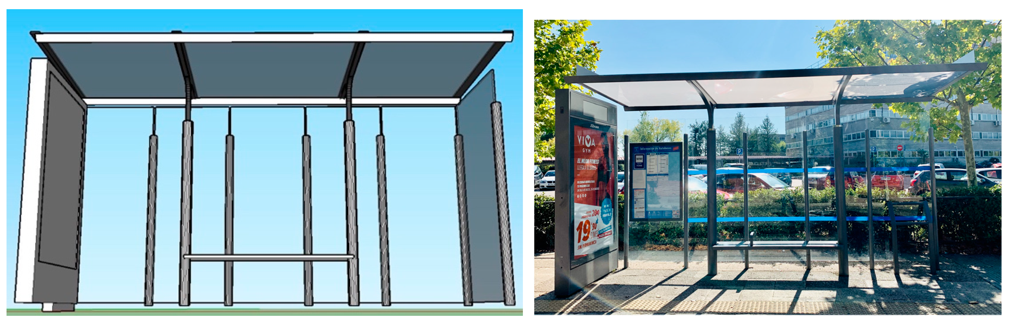
There are many lines of research and novel methodologies aimed at the extraction of road elements utilizing LiDAR [5,31]. The extraction of features allows the separate consideration of single objects and permits their evaluation, inventory, among other uses. If one wants to gauge the effect of including a particular element into the road scene, this element could be modeled and included in the geoprocessing model as another input. Additionally, if the location of an existing item of the road wants to be improved, this element could be easily removed from the model and located elsewhere so as to run the evaluation again. Elements whose evaluations are to be carried out are those within the competences of DOTs such as road utilities, public transport elements, some street furniture items, etc. These elements are predominantly surfaces and structures. The level of detail required to perform accurate evaluations is defined as medium. This means that their accurate representation is needed but no functional information is required in order to carry out the evaluation. Dimensions have to be as realistic as possible but characteristics like colors or definition of materials are not necessary. Figure 5 displays the 3D model representation of a bus stop shelter and the real element on its right. After some editing this object can accurately portray the real element and be included in the model as an input.

3.4. Vehicle Path and Target and Oobserver Heights

The vehicle path represents the different positions of the considered driver and the indicated targets. This path is represented as a set of equally spaced points holding the eye height of observer and target. As mentioned in previous sections, depending on the guidelines, the stations could be along the centerline, edge of the traveled way [1], or at fixed offsets from the centerline [2]. Also, depending on the required sight distance under evaluation, the position of the target might vary from the traveled path to opposite lanes, this also affects the considered height of the target. The indicated eye height of the observer and height of the target also vary from one standard to another.

4. Results and Discussions

The presented methodology was applied to distinct cases so as to evaluate the effect of multipatch resolution in the results. Later, relocation evaluations were carried out so as to obtain the potentials of the separate consideration of aboveground and ground elements and finally, some considerations are made regarding time and costs. In order to perform these evaluations distinct road sections were mapped utilizing MMS. The following section shows their main findings.

4.1. Effect of Multipatch Maximum Edge Lenght on the Analysis Made in a Rural Road Section

In order to perform this evaluation, a rural road section was mapped with the MMS IPS3 from Topcon [32]. This survey was planned and compiled to meet approximately ±10 mm horizontal and ±15 mm vertical accuracy at 95% confidence level. The resulting point clouds were pre-processed with software provided by the vendors. The georeferencing, denoising and classification of the cloud were performed in-house with the software MDTOPx [33]. The case study was a two-lane rural highway located in the region of Madrid (Spain). The initial point cloud comprised approximately 38 million points.

So as to evaluate the impact of the selected distance between the edges of the polyhedral entities, two files were created, one with 2 m of maximum edge length and another one with 20 cm separation. Figure 6a–d show the visual comparison of each model, both displaying a DTM of 50 cm. Figure 6a,b show an aerial oblique view of the file with 20 cm edge length.

The DTM is colored in gold and the multipatch in gray. Image 6b is a close up of 6a showing the crash barrier, road geometry and surrounding vegetation. These polygons are closer to reality, but the computational resources required to handle them were as well higher. Figure 6c,d display the multipatch file with edges as long as 2 meters. As before, an aerial oblique view is shown (6c) and from there, a close up (6d). Due to the fact that the distance between polygons is allowed to be as long as two meters, triangles were formed with vegetation, noise (current traffic) and the crash barrier. As these traffic elements were not removed during the denoise phase they were included in the model and grouped with vegetation and road elements. So as to perform the comparison between the results obtained with this model and the one of 20 cm, these elements (traffic) were removed.

Figure 7 displays the sight distance obtained with these multipatches of 2 m of maximum edge length (red line) and 20 cm separation (blue line), both with a common DTM (50 cm). The graph displays the stations along the road on the horizontal axis and the ASD of each station on the vertical one. In addition to the ASDs, the required SSDs are displayed (green line).

The SSD was obtained according to the equation provided by the Spanish geometric design standard (Equation (1)):

$$SSD=\frac{V·t_p}{3.6}+\frac{V^2}{254·\left(f_l\pm i\right)}$$

(1)

where $V$ is the vehicle’s speed at the beginning of the stopping maneuver; $t_p$ is the perception and reaction time; $f_l$ is the coefficient of longitudinal friction and $i$ is the road’s grade. The speed employed in the calculations was the posted speed limit of the road section which is 60 km/h. The perception and reaction time considered was the one stipulated in the Spanish guidelines (2 s). The coefficient of longitudinal friction, which depends on the traveling speed, was that of 0.39 for the aforementioned speed. The grades of each station were obtained from their exact coordinates.

Figure 7 shows that the ASD increases abruptly in the first stations and then it progressively decreases reaching a local minimum value between stations 103 and 109. These reduced values are due to the effect of a crest curve. From there, the impact of the horizontal curve causes sight distances to reach another minimum near station 201. These sections hold ASD values which are lower than the required SSDs. This noncompliance could impact the safety of the section negatively. Approximately 21% of the presented section (350 m) was not provided with the required SSD. Results showed that most of these visual restrictions were caused by alignment and profile curves. As the study area is located in a zone with complex topography, which restricts possible alignment modifications, adjustments to the speed limit could ensure the provisioning of the required SSD values.

Furthermore, the graph shows that the model with smaller edge length contains more variability due to the distinct effects roadside obstructions cause to each station. The evaluation performed with the 20 cm separation file lasted twice the duration of the one with 2 meters.

A statistical comparison was made between the results delivered by the two models. The Wilcoxon test performed indicated that the difference between the models is statistically significant at a level of confidence of 95% (

Table 1. Wilcoxon statistical test of results using distinct multipatch resolution.

Estimate	p-Value	Estimate	95% Confidence Interval
V = 2628	<0.0001	(Pseudo) Median = 4.499973	(3.500006, 5.999998)

).

As seen considering distances between edges up to 2 m produces larger polygons and augments the volume of the overall vegetation. This model generalizes the effect of vegetation among stations. It does not allow the verification of the specific effect that the heterogeneity of the foliage causes to the lines of sight.

4.2. Potentials of the Separate Consideration of Aboveground and Ground Elements

This evaluation was carried out in a 3-way, skewed intersection located in the city of Madrid. Here the impact of the location of a roadside element was to be done. This dataset was collected as well with the MMS IPS3 from Topcon with the same quality requirements. The required distance under evaluation was the ISD. The ISD was obtained according to Equation (2) [1]:

$$ISD=0.278V_{major}{t}_g$$

(2)

where $V_{major}$ is the design speed of the major road and t_g is the time wrap for minor road vehicle to enter the major road, which is stipulated to be 6.5 s. As the observers were considered to be cyclists the speed utilized was 35 km/h. Their required sight distance was 63.24 m.

This stop-signalized intersection was found to have a bus stop shelter near one of its turns. Due to the benefits of standardized road equipment, one bus shelter with similar measurements as the one required was found in the online warehouse of the software SketchUp (Trimble, Sunnyvale, CA, USA). This object was edited to have the dimensions and shape of the real one and included in the analysis. Figure 8 shows the lines of sight launched from an observer going down the minor road towards approaching traffic. The bus stop shelter is portrayed in white and it can be seen that it obstructs the lines of sight. After repositioning the bus stop-shelter 5 meters north-west the calculations were re-launched, delivering better results.

Figure 9 displays a 3D view of the evaluation. As in Figure 8, the gray elements depict the aboveground features. The colors of the DTM vary according to its height. A selection of the visuals showed in the previous Figure is also portrayed. Red lines represent those sightlines that were obstructed, and the green ones show those that were not. The purple points stand for the exact location where the first visual obstruction was encountered. In this case, the intersection sight distances were provisioned. As the visual obstructions were caused by a roadside element, in order to enhance the safety of the intersection its repositioning is recommended.

Regarding the resources required to carry out these evaluations, some final considerations ought to be made. In order to obtain point clouds with the sufficient accuracy and density to describe the aboveground elements, the use of terrestrial MLS is favorable. One drawback of these systems could be their direct and derived costs. These systems could range from few hundred thousand dollars, however there are many service providers offering mapping and surveying services at affordable costs if shared uses of the data are intended [18]. When it comes to time and computational resources, these depend on whether the LiDAR processing is done in-house or not. The time required by the model depends on many factors such as the considered separation between stations, the length of road under evaluation, computational resources, the type and density of roadside element present, etc. For instance, the second evaluation which comprised the functional area of the intersection, required the evaluation of a traveled way of 269 m. This trajectory was discretized into 5 m separated stations. The aboveground elements described were sparse vegetation, surrounding edifications, fences and road assets (traffic signs). The estimation of sufficient ASD to perform the stopping maneuver safely lasted 23 minutes.

5. Conclusions

The proposed methodology allowed the estimation of sight distances out of really dense point clouds. This is done by making use of a geoprocessing model that utilizes GIS tools. Newer resolutions provided by distinct MMS allow the representation of elements that could obstruct motorists’ lines of sight. The importance of evaluating the ASD on existing roads is widely acknowledged and there have been many scientific research works aimed at the elaboration of methodologies to carry out these estimations. This methodology makes use of GIS models that are accurate enough to represent the complex road scene three-dimensionally.

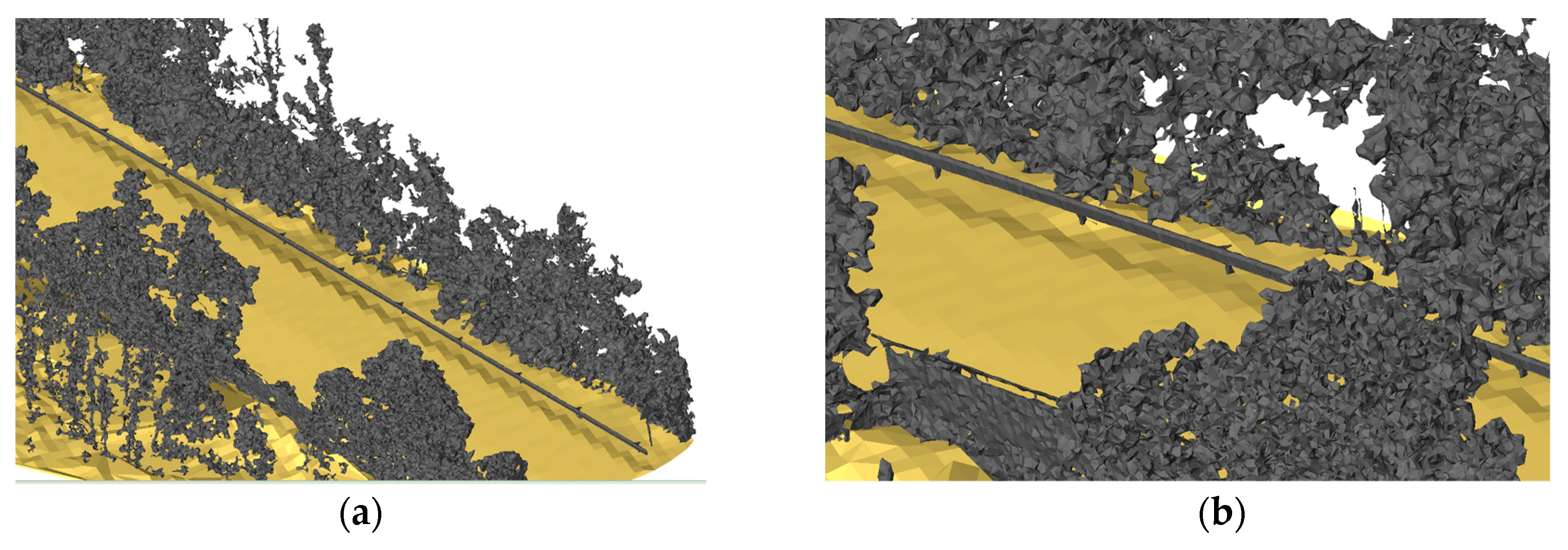
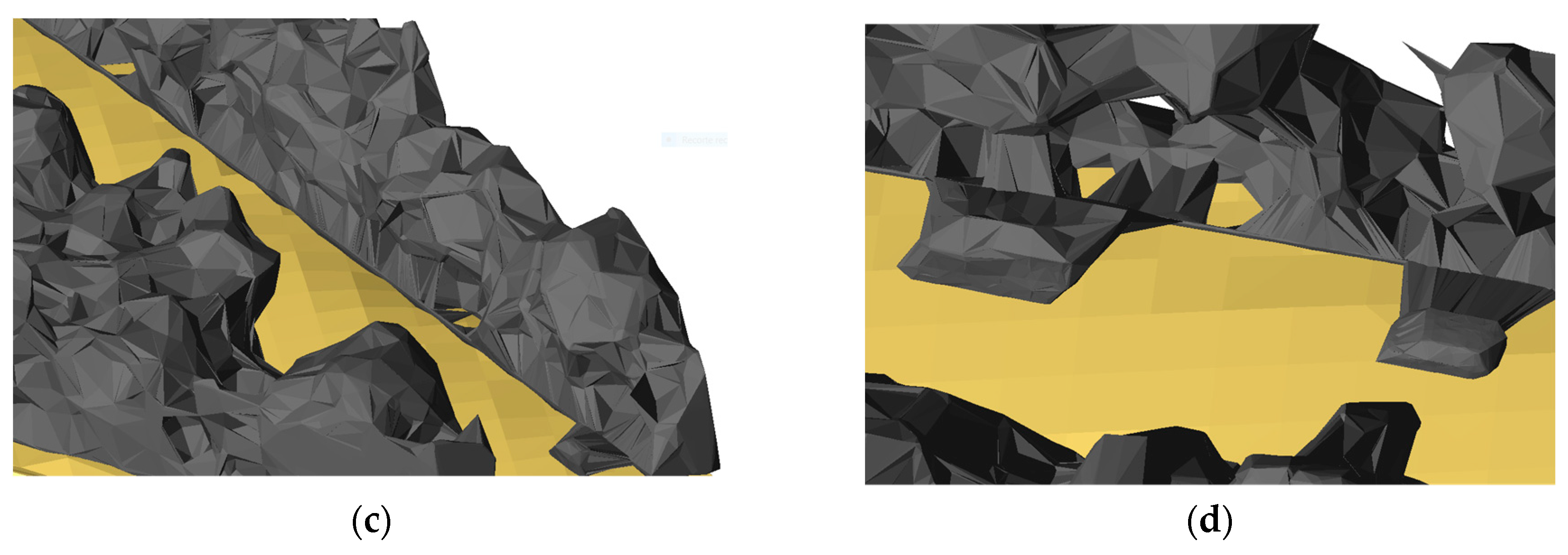
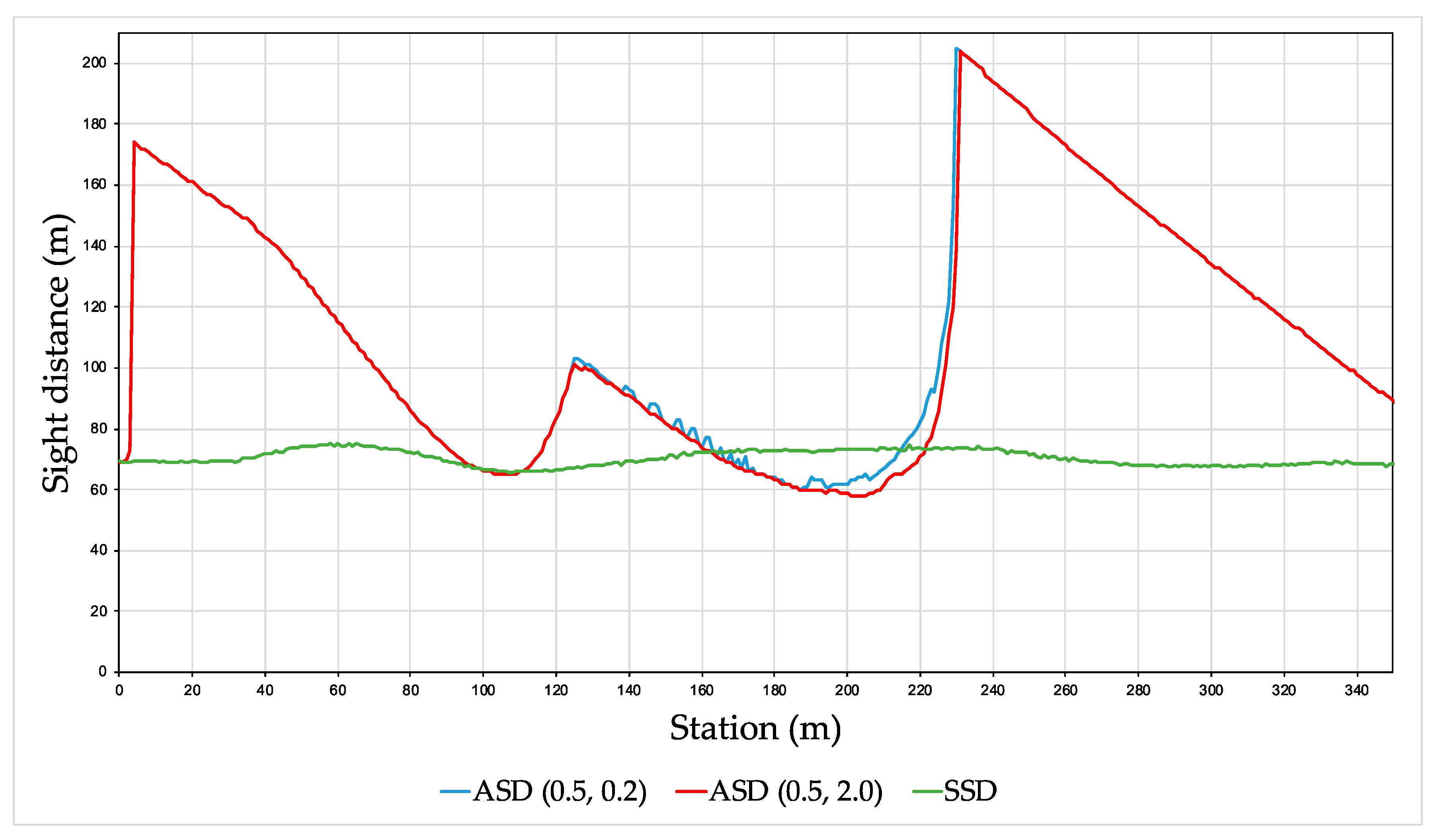
The first comparison between distinct multipatch resolutions showed that the maximum edge selected, up to 2 m, did not represent the elements surrounding the road appropriately, whereas the finest considered resolution showed more realistic features. From the statistical comparison the difference between the results delivered by the two was proved. As previously mentioned, the new densities and accuracies provided by newer MMS allow the obtention of clouds with the capability of portraying very definite elements. Accurate results require a more complex and realistic geometric representation of roadside elements. This requirement slows performance and could difficult the consideration of entire road networks.

The second evaluation included a modified 3D element. It highlighted the level of detail required from these objects to be used properly. Only geometry features impact the accuracy of the estimations whereas other semantic information could be useful but is not necessary. Future research will focus on the comparison of distinct multipatch resolutions so as to obtain those maximum edges that providing accurate representations would not represent a challenge to the available computational resources.