Change Detection of High Spatial Resolution Images Based on Region-Line Primitive Association Analysis and Evidence Fusion


Abstract

1. Introduction
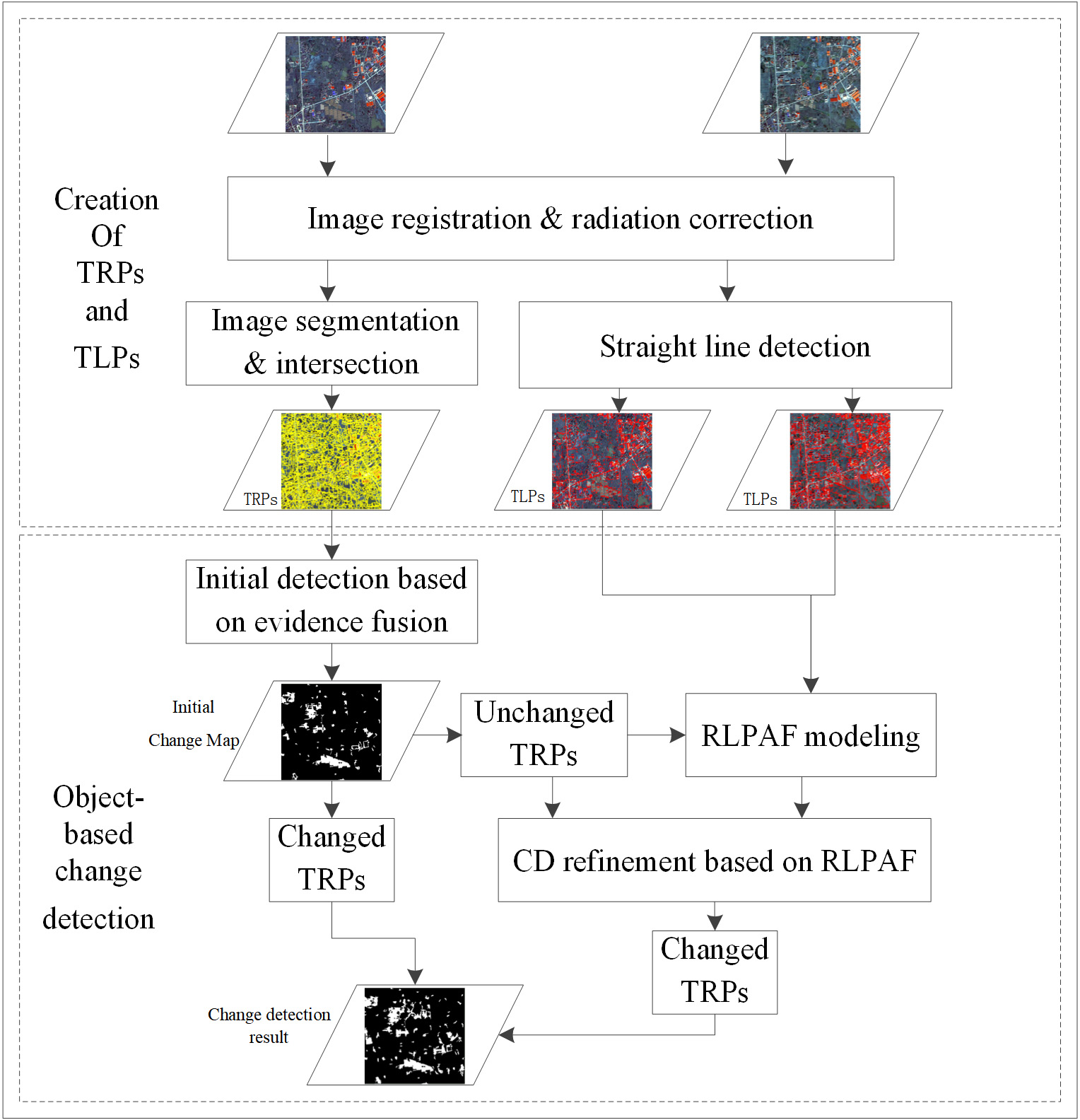
2. Methodology
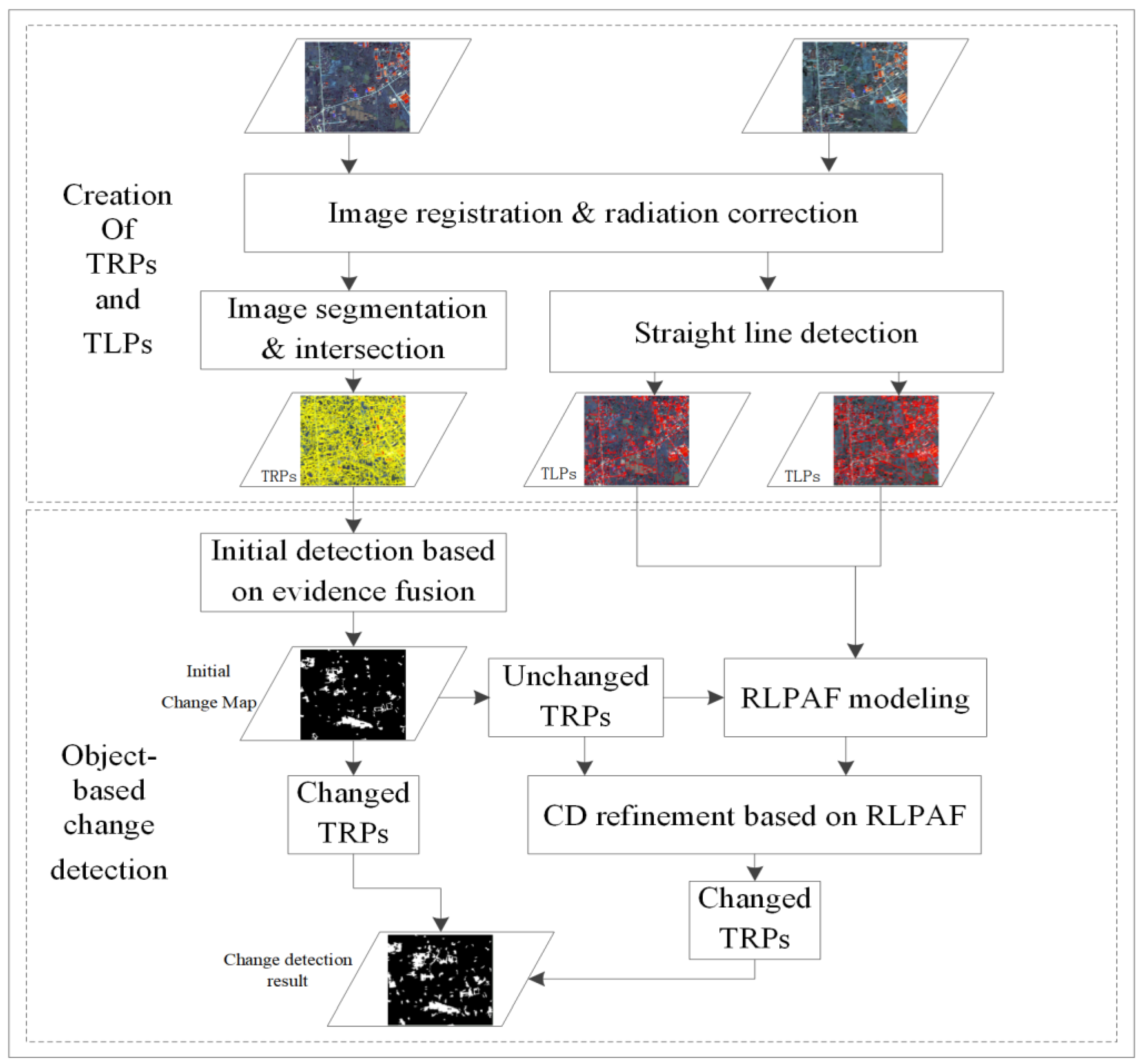
2.1. Object Primitive Creation and Change Feature Extraction
2.2. Initial Change Detection
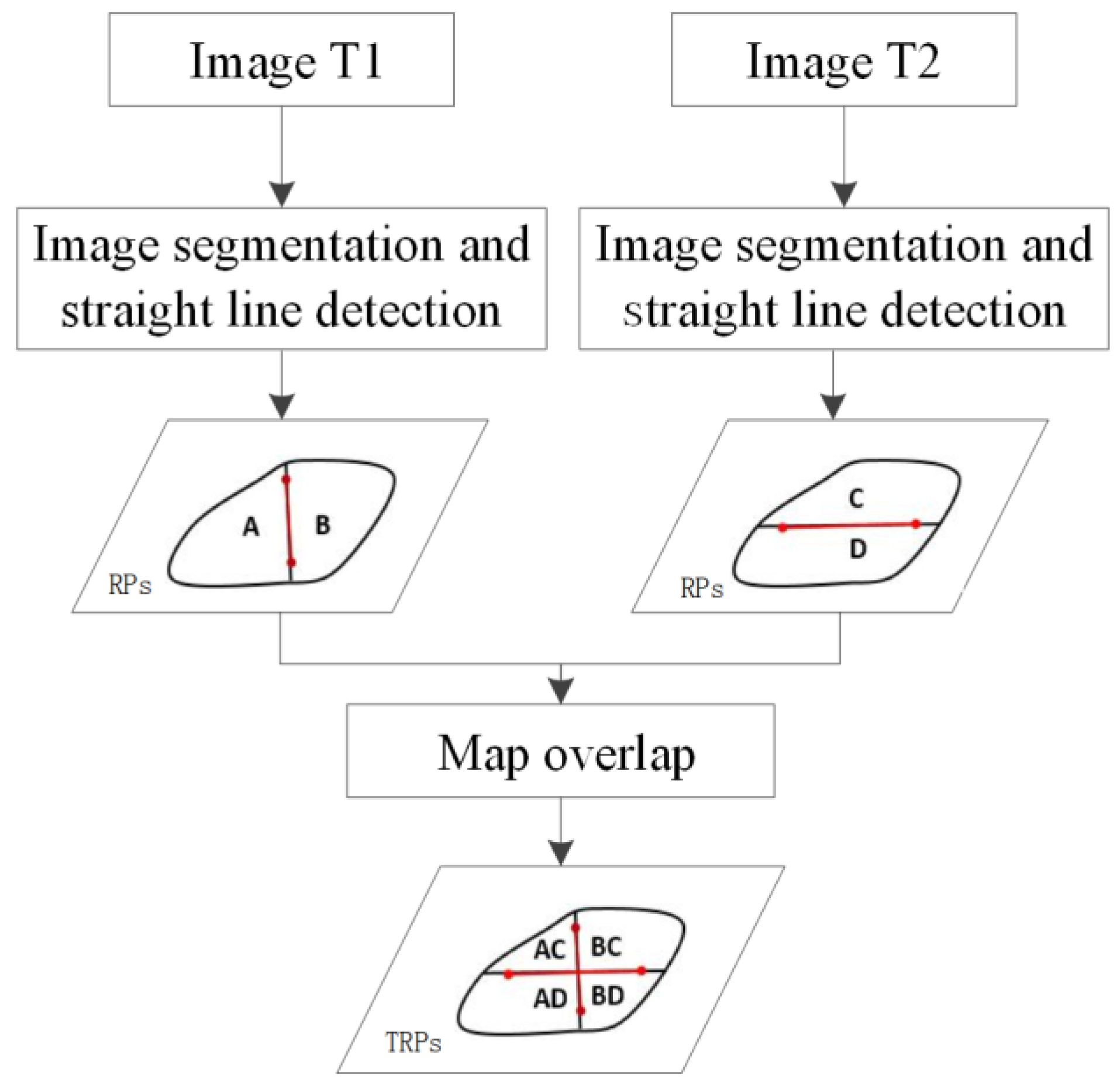
2.2.1. Feature Similarity Measure
2.2.2. Change Detection by Evidence Fusion
2.3. Change Detection Refinement Using RLPAF
| Algorithm 1. Two-stage change detection |
| Input: TRPs {P}, TLPs {L1}, and {L2}, Change threshold T, Scaling factor S Output: Changed TRPs {PC} For each P within {P}{ Calculate its spectral BPAF, gradient BPAF, and edge BPAF and fuse them to obtain BN If P’s BN < T, put P to {PC} Else Obtain P’s bitemporal MLD1 and MLD2 using its contacted lines extracted from {L1} and {L2} If MLD1 is not equal to MLD2 relax threshold T to T1 (T×S) If BN <T1, put P to {PC} Return {PC} |
3. Experimental Results and Analysis
3.1. Experimental Procedure
3.2. Method Performance Analysis
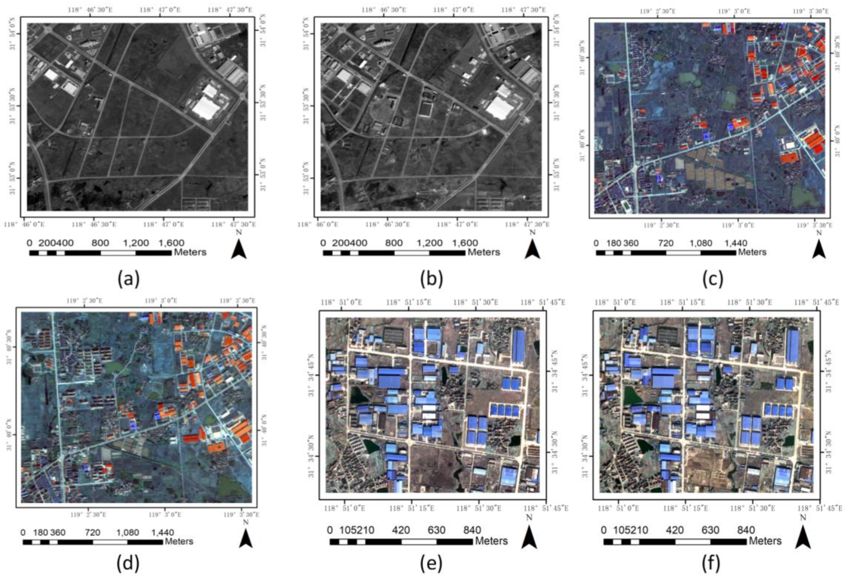
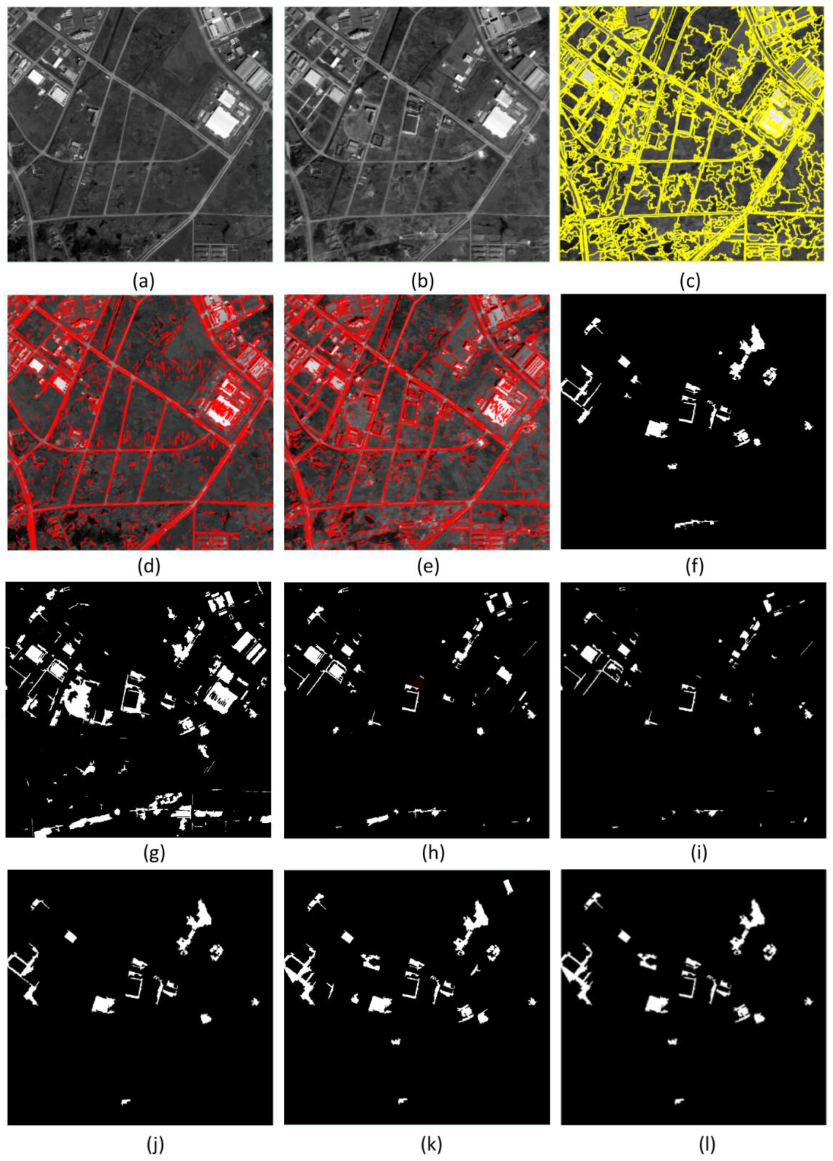
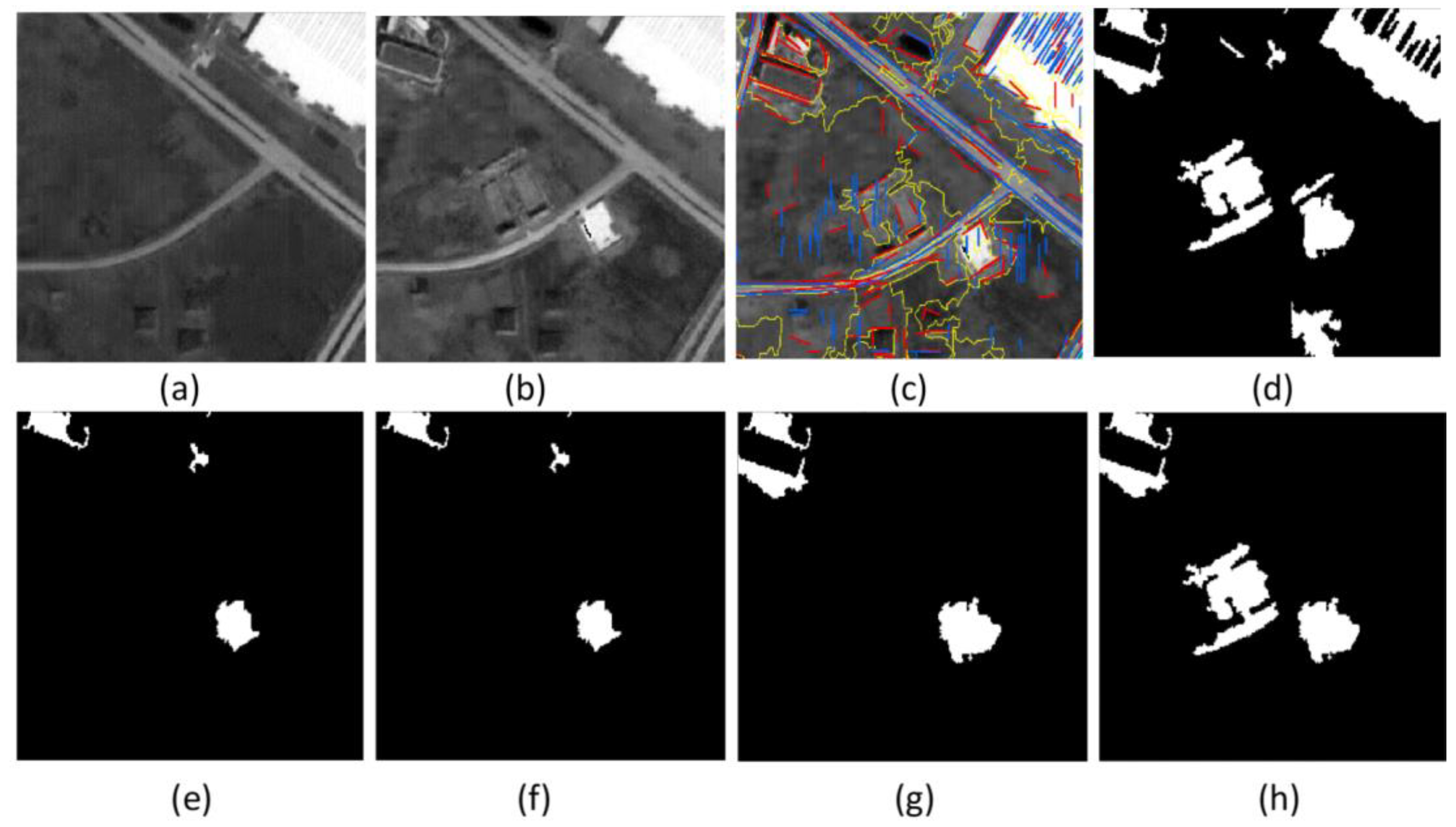
3.2.1. Experimental Area 1
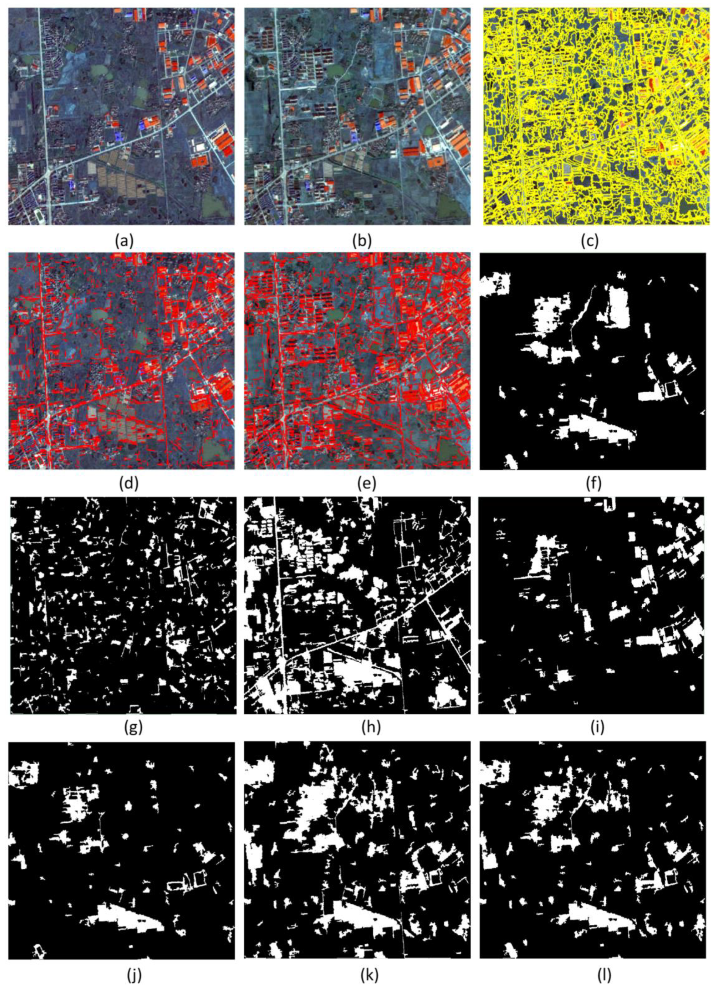
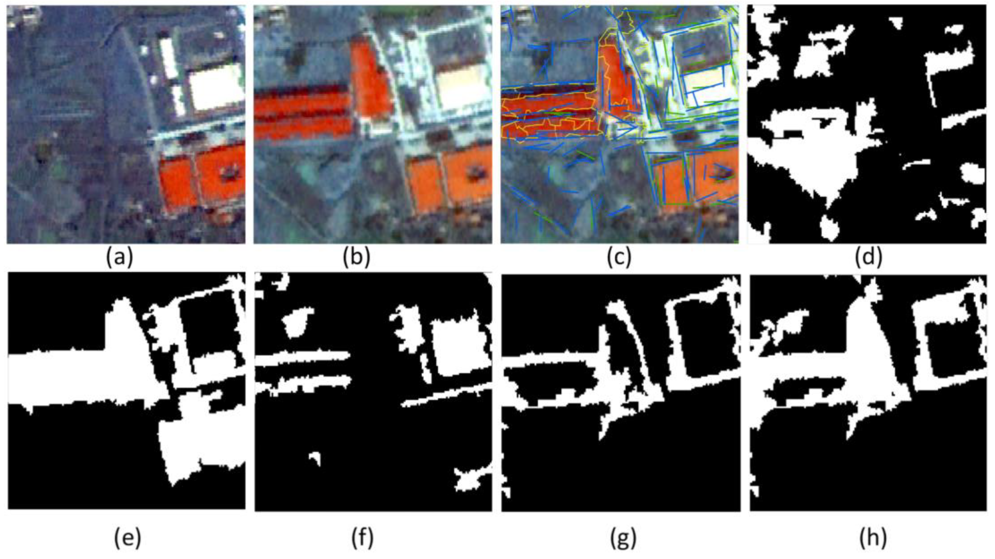
3.2.2. Experimental Area 2
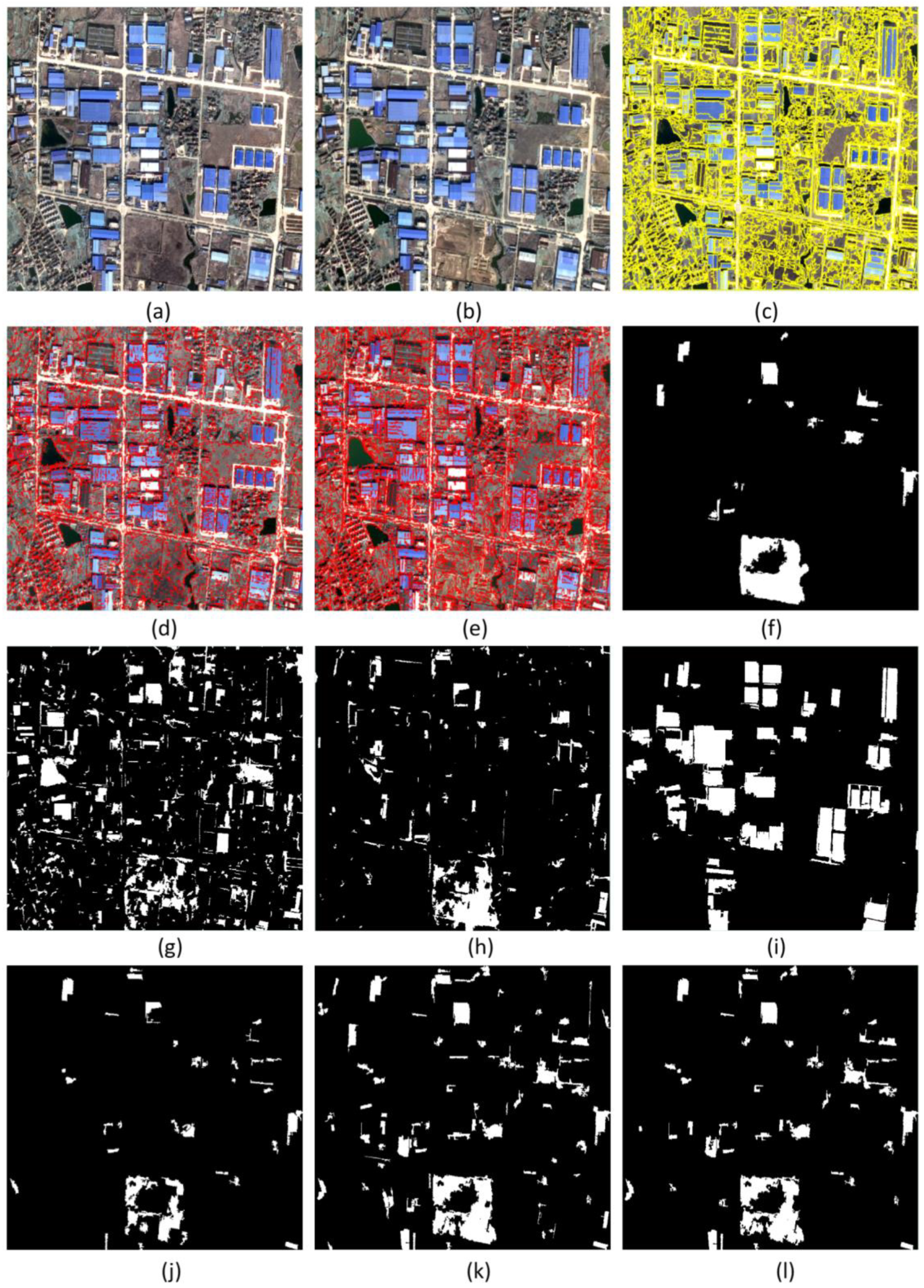
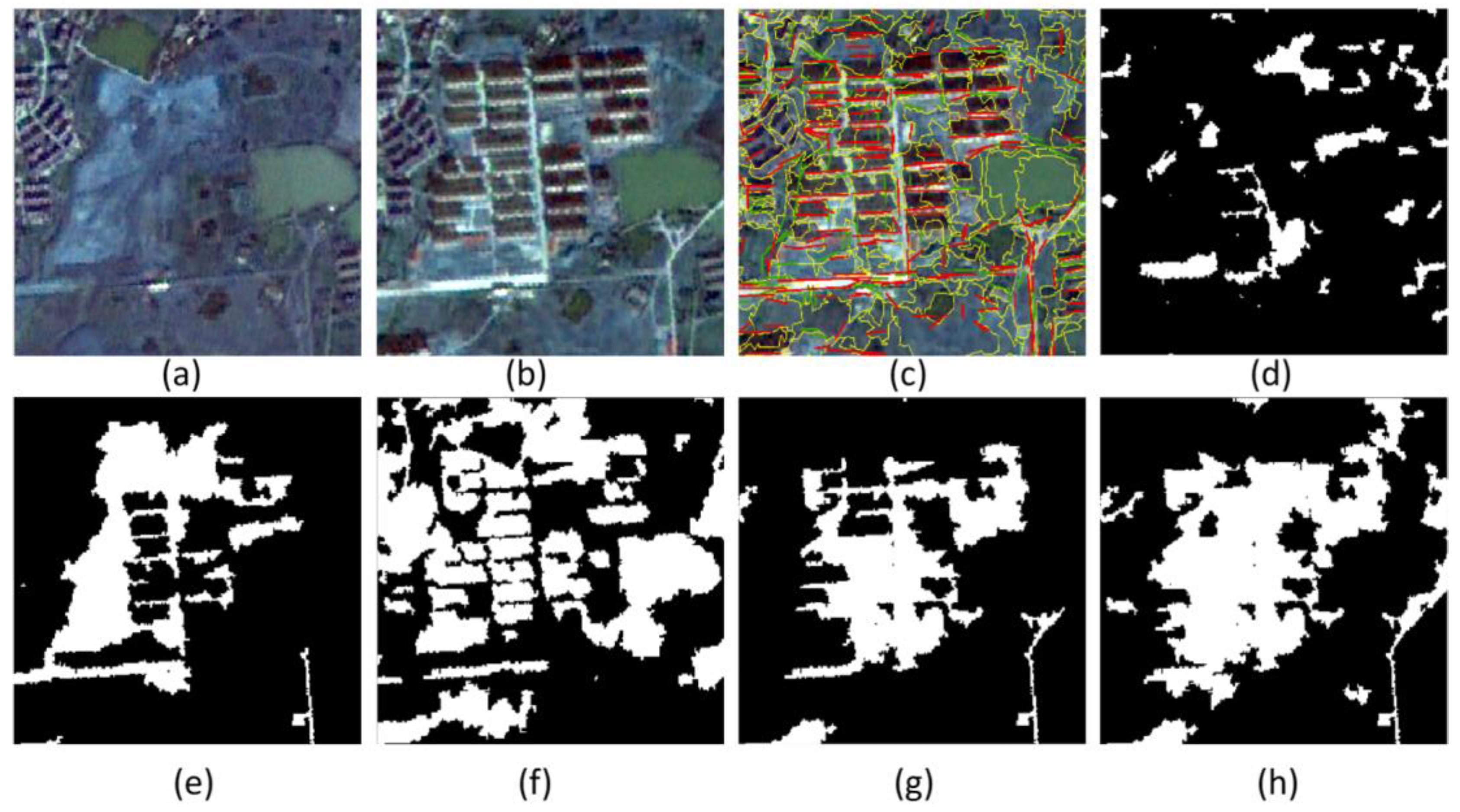
3.2.3. Experimental Area 3
3.2.4. Further Analyses
4. Discussion
4.1. Method Efficiency
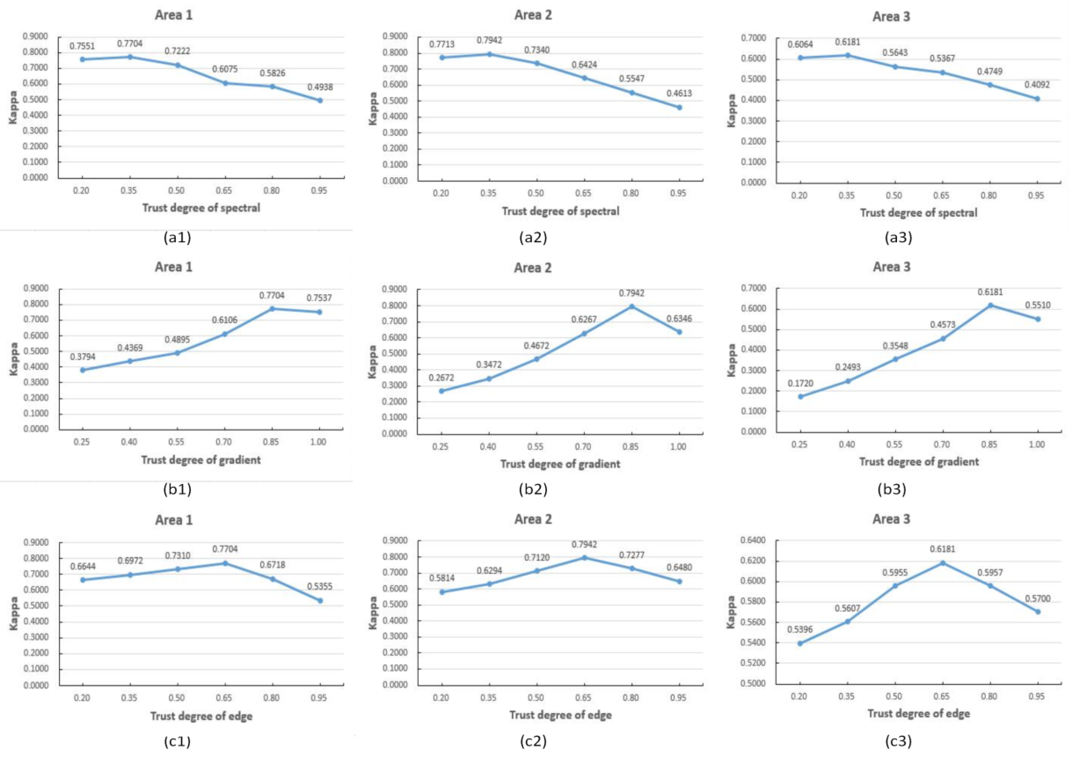
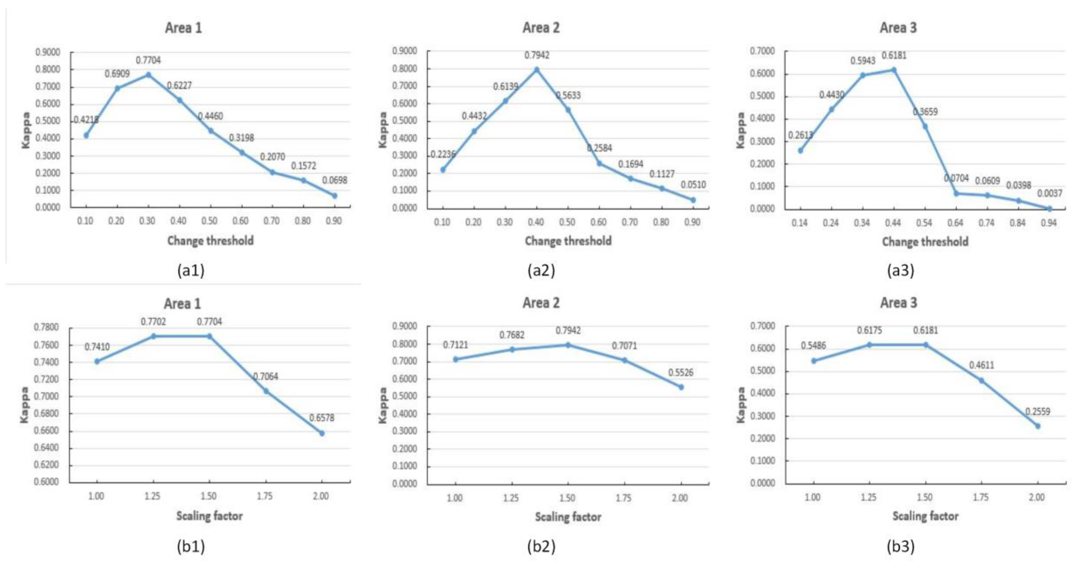
4.2. Parameter Influence
4.3. Further Discussion on Method Performance
5. Conclusions
Author Contributions
Funding
Acknowledgments
Conflicts of Interest
Abbreviations
| CD | change detection |
| HSR | high spatial resolution |
| OBCD | object-based change detection |
| TRP | temporal region primitive |
| TLP | temporal line primitive |
| MLD | main line direction |
| PBCD | pixel-based change detection |
| COCD | classification-based change detection |
| FOCD | feature-based change detection |
| HCD | hybrid change detection |
| CVA | change vector analysis |
| PCA | principal component analysis |
| MAD | multivariate alteration detection |
| IRMAD | iterative reweighted multivariate alteration detection |
| OBIA | object-based image analysis |
| D-S | Dempster and Shafer |
| ISFA | iterative slow feature analysis |
| RLPAF | region–line primitive association framework |
| LP | line primitive |
| RP | region primitive |
| SSIM | structural similarities |
| BPAF | basic probability assignment function |
| GDAL | Geospatial Data Abstraction Library |
| ALOS | Advanced Land Observation Satellite |
| PRISM | panchromatic Remote-Sensing Instrument for Stereo Mapping |
| AVNIR-2 | advanced Visible and Near-Infrared Radiometer 2 |
| FA | false alarm |
| MA | missed alarm |
| OA | overall accuracy |
References
- Singh, A. Digital change detection techniques using remotely sensed data. Int. J. Remote. Sens. 1989, 10, 989–1003. [Google Scholar] [CrossRef]
- Lu, D.; Mausel, P.; Brondízio, E.; Moran, E. Change detection techniques. Int. J. Remote Sens. 2004, 25, 2365–2401. [Google Scholar] [CrossRef]
- Chen, G.; Hay, G.J.; Carvalho, L.M.T.; Wulder, M.A. Object-based change detection. Int. J. Remote Sens. 2012, 33, 4434–4457. [Google Scholar] [CrossRef]
- Hussain, M.; Chen, D.; Cheng, A.; Wei, H.; Stanley, D. Change detection from remotely sensed images: From pixel-based to object-based approaches. ISPRS J. Photogramm. Remote Sens. 2013, 80, 91–106. [Google Scholar] [CrossRef]
- Chen, Q.; Chen, Y. Multi-Feature Object-Based Change Detection Using Self-Adaptive Weight Change Vector Analysis. Remote Sens. 2016, 8, 549. [Google Scholar] [CrossRef]
- Lamine, S.; Petropoulos, G.P.; Singh, S.K.; Szabó, S.; Bachari, N.; Srivastava, P.K.; Suman, S. Quantifying Land Use/Land Cover Spatio-Temporal Landscape Pattern Dynamics from Hyperion Using SVMs Classifier and FRAGSTATS®. Geocarto Int. 2017, 33, 862–878. [Google Scholar] [CrossRef]
- Bruzzone, L.; Prieto, D.F. Automatic analysis of the difference image for unsupervised change detection. IEEE Trans. Geosci. Remote Sens. 2000, 38, 1171–1182. [Google Scholar] [CrossRef]
- Nemmour, H.; Chibani, Y. Multiple support vector machines for land cover change detection: An application for mapping urban extensions. ISPRS J. Photogramm. Remote Sens. 2006, 61, 125–133. [Google Scholar] [CrossRef]
- Bovolo, F.; Bruzzone, L. A Theoretical Framework for Unsupervised Change Detection Based on Change Vector Analysis in the Polar Domain. IEEE Trans. Geosci. Remote Sens. 2007, 45, 218–236. [Google Scholar] [CrossRef]
- Dai, Q.; Liu, J.; Liu, S. Remote sensing image change detection using particle swarm optimization algorithm. Acta Geod. Cartogr. Sin. 2012, 41, 847–850. [Google Scholar]
- Su, J.; Liu, D. An Object-level change detection algorithm for remote sensing images. Acta Photonica Sin. 2007, 36, 1764–1768. [Google Scholar]
- Wang, W.; Zhao, Z.; Zhu, H. Object-oriented multi-feature fusion change detection method for high resolution remote sensing image. In Proceedings of the 17th International Conference on Geoinformatics, Fairfax, VA, USA, 12–14 August 2009. [Google Scholar]
- Wu, J.; Yan, W.; Ni, W.; Hui, B. Object-Level Change Detection Based on Image Fusion and Multi-Scale Segmentation. Electron. Opt. Cont. 2013, 20, 51–55. [Google Scholar]
- Lv, X.; Ming, D.; Lu, T.; Zhou, K.; Wang, M.; Bao, H. A new method for region-Based majority voting CNNs for very high resolution image classification. Remote Sens. 2018, 10, 1946. [Google Scholar] [CrossRef]
- Peng, D.; Zhang, Y. Object-based change detection from satellite imagery by segmentation optimization and multi-features fusion. Int. J. Remote Sens. 2017, 38, 3886–3905. [Google Scholar] [CrossRef]
- Sun, K.; Chen, Y. The Application of Objects Change Vector Analysis in Object-level Change Detection. In Proceedings of the 3rd International Conference on Computational Intelligence and Industrial Application (PACIIA 2010), Wuhan, China, 6–7 November 2010; pp. 383–389. [Google Scholar]
- Wang, C.; Xu, M.; Wang, X.; Zheng, S.; Ma, Z. Object-oriented change detection approach for high-resolution remote sensing images based on multiscale fusion. J. Appl. Remote Sens. 2013, 7, 073696. [Google Scholar] [CrossRef]
- Hazel, G.G. Object-level change detection in spectral imagery. IEEE Trans. Geosci. Remote Sens. 2001, 39, 553–561. [Google Scholar] [CrossRef]
- Su, X.; Wu, W.; Li, H.; Han, Y. Land-Use and Land-Cover Change Detection Based on Object-Oriented Theory. In Proceedings of the 2011 International Symposium on Image and Data Fusion, Tengchong, China, 9–11 August 2011. [Google Scholar]
- Ming, D.; Zhou, W.; Xu, L.; Wang, M.; Ma, Y. Coupling relationship among scale parameter, segmentation accuracy and classification accuracy In GeOBIA. Photogramm. Eng. Remote Sens. 2018, 84, 681–693. [Google Scholar] [CrossRef]
- Zhang, L.; Wu, C. Advance and Future Development of Change Detection for Multi-temporal Remote Sensing Imagery. Acta Geod. Cartogr. Sin. 2017, 46, 1447–1459. [Google Scholar]
- Malila, W.A. Change vector analysis: An approach for detecting forest changes with Landsat. In Proceedings of the 1980 Machine Processing of Remotely Sensed Data Symposium, West Lafayette, IN, USA, 3–6 June 1980; pp. 326–335. [Google Scholar]
- Celik, T. Unsupervised Change Detection in Satellite Images Using Principal Component Analysis and k-Means Clustering. IEEE Geosci. Remote Sens. Lett. 2009, 6, 772–776. [Google Scholar] [CrossRef]
- Nielsen, A.A.; Conradsen, K.; Simpson, J.J. Multivariate Alteration Detection (MAD) and MAF Postprocessing in Multispectral, Bitemporal Image Data: New Approaches to Change Detection Studies. Remote Sens. Environ. 1998, 64, 1–19. [Google Scholar] [CrossRef]
- Nielsen, A.A. The Regularized Iteratively Reweighted MAD Method for Change Detection in Multi- and Hyperspectral Data. IEEE T. Image Process. 2007, 16, 463–478. [Google Scholar] [CrossRef]
- Du, X.; Zhang, C.; Yang, J.; Su, W. A New Multi-Feature Approach to Object-Oriented Change Detection Based on Fuzzy Classification. Intell. Autom. Soft Comput. 2012, 18, 1063–1073. [Google Scholar] [CrossRef]
- Tang, Y.; Huang, X.; Zhang, L. Fault-Tolerant Building Change Detection from Urban High-Resolution Remote Sensing Imagery. IEEE Geosci. Remote Sens. Lett. 2013, 10, 1060–1064. [Google Scholar] [CrossRef]
- Chen, Q.; Chen, Y.; Jiang, W. Genetic Particle Swarm Optimization–Based Feature Selection for Very-High-Resolution Remotely Sensed Imagery Object Change Detection. Sensors 2016, 16, 1204. [Google Scholar] [CrossRef] [PubMed]
- Zhang, B.; Lu, J.; Guo, H.; Xu, J.; Zhao, C. Object-oriented change detection for multi-source images using multi-feature fusion. In Proceedings of the 2016 Third International Conference on Artificial Intelligence and Pattern Recognition (AIPR), Lodz, Poland, 19–21 September 2016. [Google Scholar]
- Cai, L.; Shi, W.; Hao, M.; Zhang, H.; Gao, L. A Multi-Feature Fusion-Based Change Detection Method for Remote Sensing Images. J. Indian Soc. Remote Sens. 2018, 46, 2015–2022. [Google Scholar] [CrossRef]
- Wang, X.; Liu, S.; Du, P.; Liang, H.; Xia, J.; Li, Y. Object-Based Change Detection in Urban Areas from High Spatial Resolution Images Based on Multiple Features and Ensemble Learning. Remote Sens. 2018, 10, 276. [Google Scholar] [CrossRef]
- Luo, H.; Liu, C.; Wu, C.; Guo, X. Urban Change Detection Based on Dempster–Shafer Theory for Multitemporal Very High-Resolution Imagery. Remote Sens. 2018, 10, 980. [Google Scholar] [CrossRef]
- Wang, M.; Wang, J. A region-line primitive association framework for object-based remote sensing image analysis. Photogramm. Eng. Remote Sens. 2016, 82, 149–159. [Google Scholar] [CrossRef]
- Wang, M.; Xing, J.; Wang, J.; Lv, G. Technical design and system implementation of region-line primitive association framework. ISPRS J. Photogramm. Remote Sens. 2017, 130, 202–216. [Google Scholar] [CrossRef]
- Wang, M.; Cui, Q.; Wang, J.; Ming, D.; Lv, G. Raft cultivation area extraction from high resolution remote sensing imagery by fusing multi-scale region-line primitive association features. ISPRS J. Photogramm. Remote Sens. 2017, 123, 104–113. [Google Scholar] [CrossRef]
- Wang, M.; Cui, Q.; Sun, Y.; Wang, Q. Photovoltaic Panel Extraction from Very High-Resolution Aerial Imagery Using Region-Line Primitive Association Analysis and Template Matching. ISPRS J. Photogramm. Remote Sens. 2018, 141, 100–111. [Google Scholar] [CrossRef]
- Wang, M.; Li, R. Segmentation of high spatial resolution remote sensing imagery based on hard-boundary constraint and two-stage merging. IEEE Trans. Geosci. Remote Sens. 2014, 52, 5712–5725. [Google Scholar] [CrossRef]
- Wang, M.; Zhang, X. Change detection using high spatial resolution remotely sensed imagery by combining evidence theory and structural similarity. J. Remote Sens. 2010, 14, 558–570. [Google Scholar]
- Burns, J.B.; Hanson, A.R.; Riseman, E.M. Extracting straight lines. IEEE Trans. Pattern Anal. Mach. Intell 1986, 8, 425–455. [Google Scholar] [CrossRef]
- Wang, Z.; Lu, L.; Bovik, A.C. Video quality assessment based on structural distortion measurement. Signal Process-Image 2004, 19, 121–132. [Google Scholar] [CrossRef]
- Ruthven, I.; Lalmas, M. Using Dempster-Shafer’s Theory of Evidence to Combine Aspects of Information Use. J. Intell. Inf. Syst. 2002, 19, 267–301. [Google Scholar] [CrossRef]
- Laben, C.A.; Brower, B.V. Process for enhancing the spatial resolution of multispectral imagery using pan-sharpening. U.S. Patent 6,011,875, 4 January 2000. [Google Scholar]
- Mattoccia, S.; Tombari, F.; Stefano, L.D. Efficient template matching for multi-channel images. Pattern Recogn. Lett. 2011, 32, 694–700. [Google Scholar] [CrossRef]


| Experimental Area | Image Type | Resolution | Imaging Date 1 | Imaging Date 2 | Image Size | Location | Segmentation Scales | Change Threshold |
|---|---|---|---|---|---|---|---|---|
| Area 1 | ALOS panchromatic image | 2.5 m | 2007.02 | 2008.01 | 999×963 | 31°52′45.40″N– 31°54′4.47″N 118°46′2.58″E– 118°47′35.97″E | 50 | 0.3 |
| Area 2 | ALOS fused image | 2.5 m | 2007.02 | 2008.01 | 885×748 | 31°39′35.516″N– 31°40′42.018″N 119°2′4.997″E~ 119°3′33.694″E | 50 | 0.4 |
| Area 3 | Gaofen-2 fused image | 1 m | 2016.02 | 2017.01 | 1576×1219 | 31°34′22.535″N– 31°34′55.646″N 118°50′56.279″E– 118°51′43.373″E | 150 | 0.44 |
| Type | Method | TP | FP | FN | TN | OA (%) | MA (%) | FA (%) | Kappa |
|---|---|---|---|---|---|---|---|---|---|
| Segment-based | CVA | 52 | 219 | 21 | 1000 | 81.42% | 28.77% | 20.82% | 0.23 |
| IRMAD | 41 | 50 | 32 | 1169 | 93.65% | 43.84% | 4.13% | 0.47 | |
| PCA-K-means | 44 | 78 | 29 | 1141 | 91.72% | 39.73% | 6.58% | 0.41 | |
| Initial detection | 49 | 8 | 24 | 1211 | 97.52% | 32.88% | 0.63% | 0.74 | |
| Direct threshold relaxation | 54 | 19 | 19 | 1200 | 97.06% | 26.03% | 1.52% | 0.72 | |
| Refined detection | 54 | 11 | 19 | 1208 | 97.68% | 26.03% | 0.87% | 0.77 | |
| Pixel-based | CVA | 20,106 | 69,808 | 10,659 | 861,464 | 91.64% | 34.65% | 7.92% | 0.30 |
| IRMAD | 11,567 | 8102 | 19,198 | 923,170 | 97.16% | 62.40% | 0.87% | 0.44 | |
| PCA-K-means | 13,116 | 15,622 | 17,649 | 915,650 | 96.54% | 57.37% | 1.68% | 0.42 | |
| Initial detection | 24,433 | 1632 | 6332 | 929,640 | 99.17% | 20.58% | 0.17% | 0.86 | |
| Direct threshold relaxation | 27,712 | 8520 | 3053 | 922,752 | 98.80% | 9.92% | 0.90% | 0.82 | |
| Refined detection | 27,712 | 5480 | 3053 | 925,792 | 99.11% | 9.92% | 0.57% | 0.86 |
| Type | Method | TP | FP | FN | TN | OA (%) | MA (%) | FA (%) | Kappa |
|---|---|---|---|---|---|---|---|---|---|
| Segment-based | CVA | 89 | 674 | 294 | 2060 | 68.94% | 76.76% | 31.36% | −0.01 |
| IRMAD | 125 | 283 | 258 | 2451 | 82.64% | 67.36% | 10.99% | 0.22 | |
| PCA-K-means | 143 | 832 | 240 | 1902 | 65.61% | 62.66% | 40.68% | 0.04 | |
| Initial detection | 253 | 45 | 130 | 2689 | 94.39% | 33.94% | 1.53% | 0.71 | |
| Direct threshold relaxation | 352 | 354 | 31 | 2380 | 87.65% | 8.09% | 12.96% | 0.58 | |
| Refined detection | 335 | 98 | 48 | 2636 | 95.32% | 12.53% | 3.30% | 0.79 | |
| Pixel-based | CVA | 13,096 | 55,495 | 60,401 | 533,873 | 82.52% | 82.18% | 10.15% | 0.09 |
| IRMAD | 20,313 | 42,380 | 53,184 | 546,988 | 85.58% | 72.36% | 7.47% | 0.22 | |
| PCA-K-means | 30,419 | 142,396 | 43,078 | 446,972 | 72.02% | 58.61% | 29.83% | 0.11 | |
| Initial detection | 45,567 | 8452 | 27,930 | 580,916 | 94.51% | 38.00% | 1.35% | 0.69 | |
| Direct threshold relaxation | 65,405 | 56,377 | 8092 | 532,991 | 90.27% | 11.01% | 9.42% | 0.62 | |
| Refined detection | 62,352 | 22,070 | 11,145 | 567,298 | 94.99% | 15.16% | 3.51% | 0.76 |
| Type | Method | TP | FP | FN | TN | OA (%) | MA (%) | FA (%) | Kappa |
|---|---|---|---|---|---|---|---|---|---|
| Segment-based | CVA | 123 | 1018 | 154 | 2710 | 70.74% | 55.60% | 35.93% | 0.07 |
| IRMAD | 16 | 419 | 261 | 3309 | 83.02% | 94.22% | 12.60% | -0.04 | |
| PCA-K-means | 145 | 342 | 132 | 3386 | 88.16% | 47.65% | 9.69% | 0.32 | |
| Initial detection | 138 | 65 | 139 | 3663 | 94.91% | 50.18% | 1.71% | 0.55 | |
| Direct threshold relaxation | 221 | 289 | 56 | 3439 | 91.39% | 20.22% | 7.90% | 0.52 | |
| Refined detection | 199 | 139 | 78 | 3589 | 94.58% | 28.16% | 3.67% | 0.62 | |
| Pixel-based | CVA | 36,450 | 242,847 | 68,541 | 1,573,306 | 85.35% | 65.28% | 12.98% | 0.14 |
| IRMAD | 12,600 | 283,041 | 92,391 | 1,533,112 | 80.46% | 87.99% | 18.31% | −0.02 | |
| PCA-K-means | 56,017 | 70,690 | 48,974 | 1,745,463 | 93.77% | 46.65% | 3.92% | 0.45 | |
| Initial detection | 49,976 | 20,372 | 55,015 | 1,795,781 | 96.08% | 52.40% | 1.10% | 0.55 | |
| Direct threshold relaxation | 89,191 | 80,469 | 15,800 | 1,735,684 | 94.99% | 15.05% | 4.41% | 0.62 | |
| Refined detection | 81,419 | 50,193 | 23,572 | 1,765,960 | 96.16% | 22.45% | 2.72% | 0.67 |
| Area | TRP and TLP Creation | Feature similarity Calculation | CD by Evidence Fusion | CD Refinement Using RLPAF |
|---|---|---|---|---|
| Area 1 | 84.78 | 7.7 | 1.06 | 13.99 |
| Area 2 | 89.84 | 23.27 | 1.19 | 24.25 |
| Area 3 | 138.09 | 29.56 | 1.49 | 117.93 |
© 2019 by the authors. Licensee MDPI, Basel, Switzerland. This article is an open access article distributed under the terms and conditions of the Creative Commons Attribution (CC BY) license (http://creativecommons.org/licenses/by/4.0/).
Share and Cite
Huang, J.; Liu, Y.; Wang, M.; Zheng, Y.; Wang, J.; Ming, D. Change Detection of High Spatial Resolution Images Based on Region-Line Primitive Association Analysis and Evidence Fusion. Remote Sens. 2019, 11, 2484. https://doi.org/10.3390/rs11212484
Huang J, Liu Y, Wang M, Zheng Y, Wang J, Ming D. Change Detection of High Spatial Resolution Images Based on Region-Line Primitive Association Analysis and Evidence Fusion. Remote Sensing. 2019; 11(21):2484. https://doi.org/10.3390/rs11212484
Chicago/Turabian StyleHuang, Jiru, Yang Liu, Min Wang, Yalan Zheng, Jie Wang, and Dongping Ming. 2019. "Change Detection of High Spatial Resolution Images Based on Region-Line Primitive Association Analysis and Evidence Fusion" Remote Sensing 11, no. 21: 2484. https://doi.org/10.3390/rs11212484
APA StyleHuang, J., Liu, Y., Wang, M., Zheng, Y., Wang, J., & Ming, D. (2019). Change Detection of High Spatial Resolution Images Based on Region-Line Primitive Association Analysis and Evidence Fusion. Remote Sensing, 11(21), 2484. https://doi.org/10.3390/rs11212484