Detecting Winter Wheat Irrigation Signals Using SMAP Gridded Soil Moisture Data


Abstract

1. Introduction
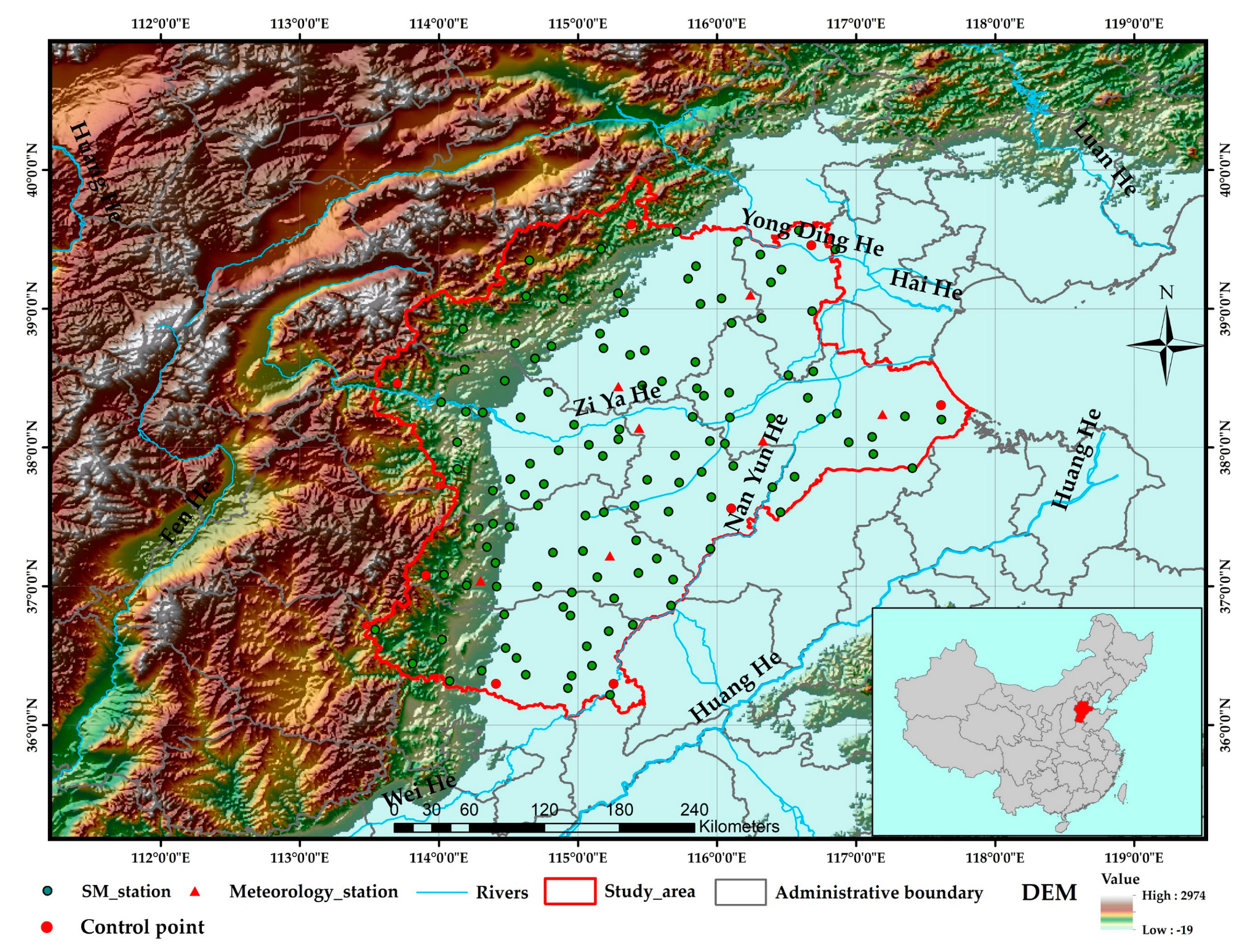
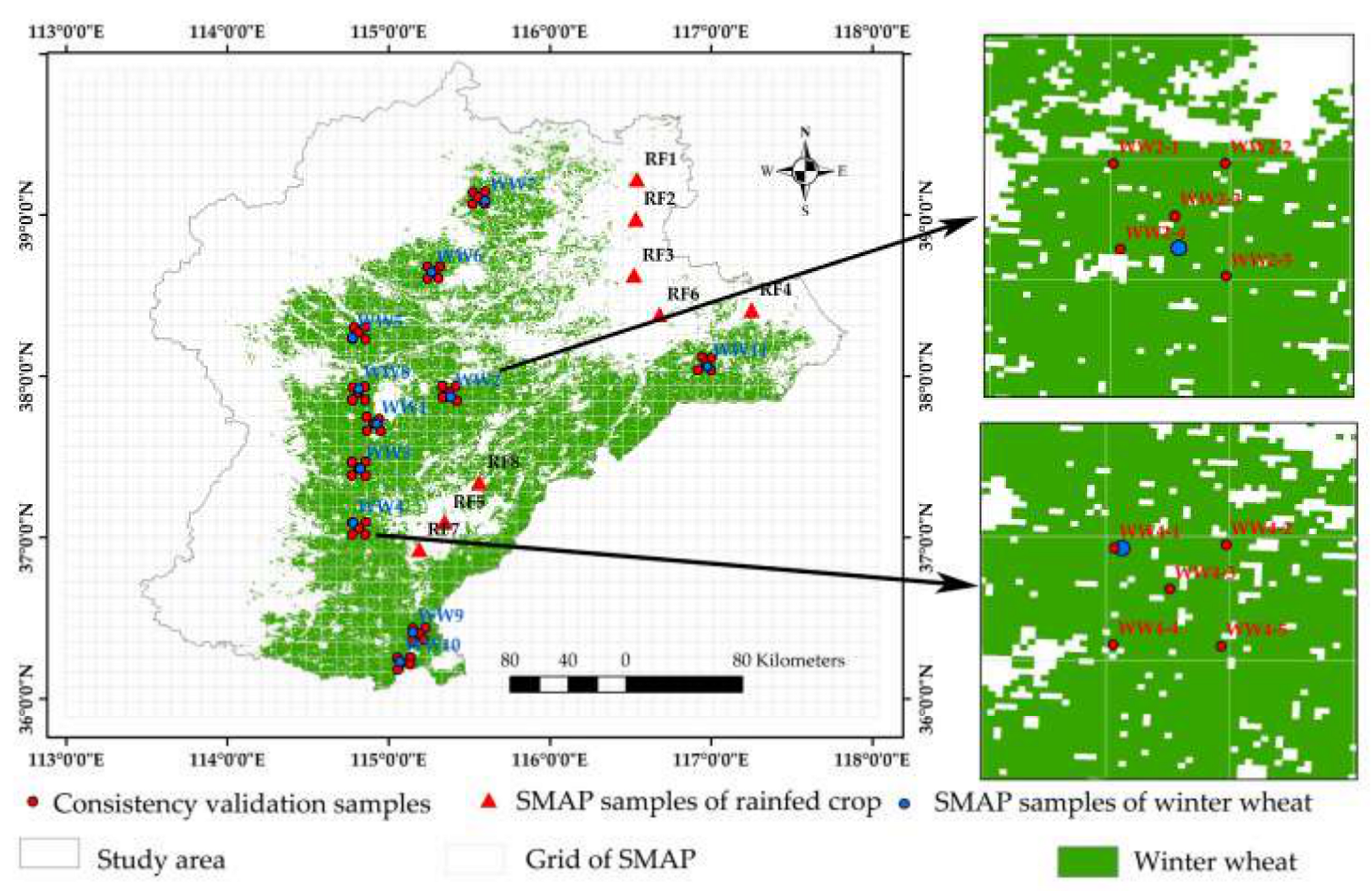
2. Study Area
3. Materials and Methods
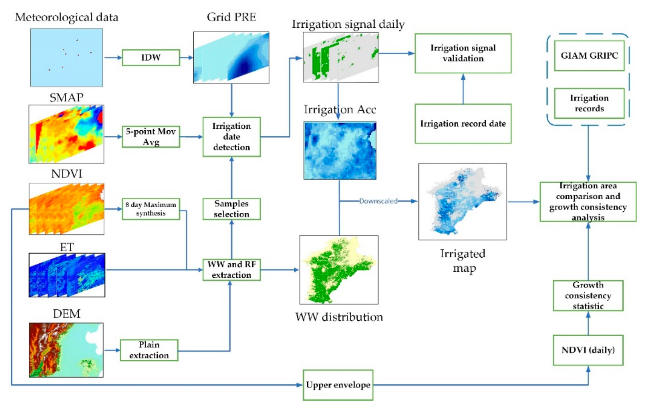
3.1. Data Collection and Pre-Processing
3.1.1. SMAP
3.1.2. MODIS
3.1.3. Precipitation
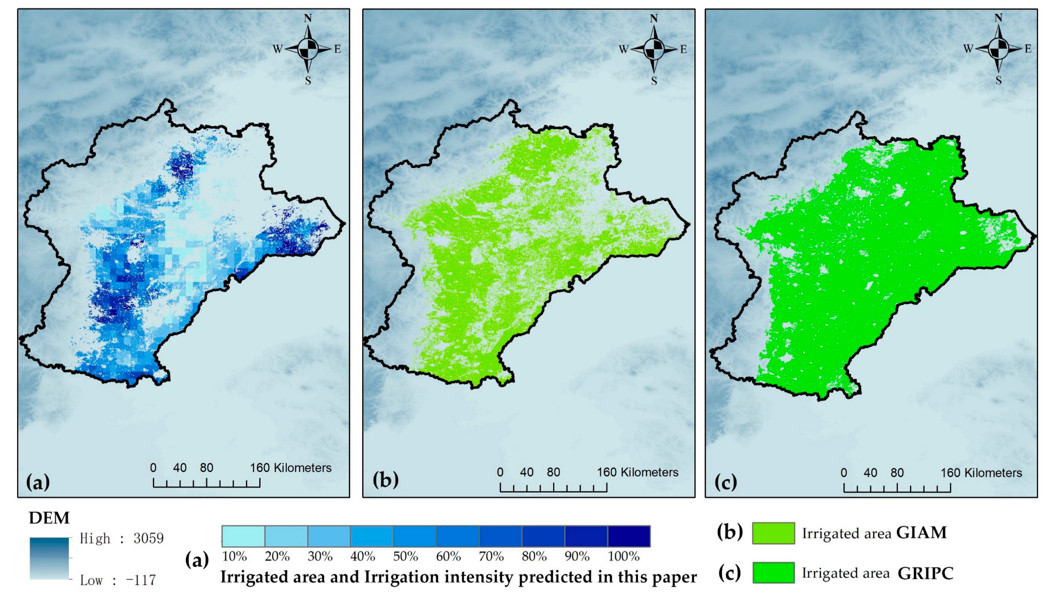
3.1.4. Irrigated Map
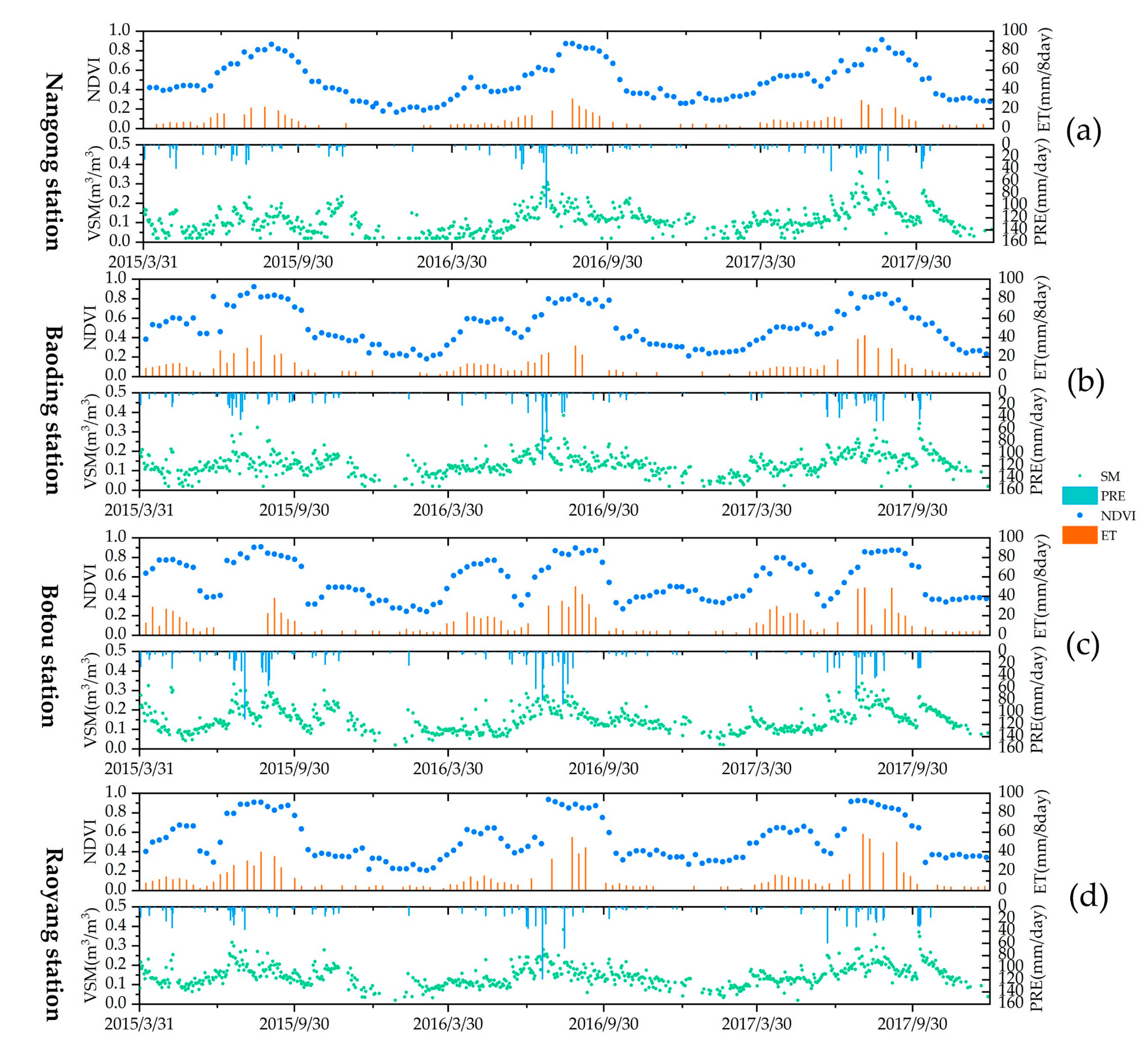
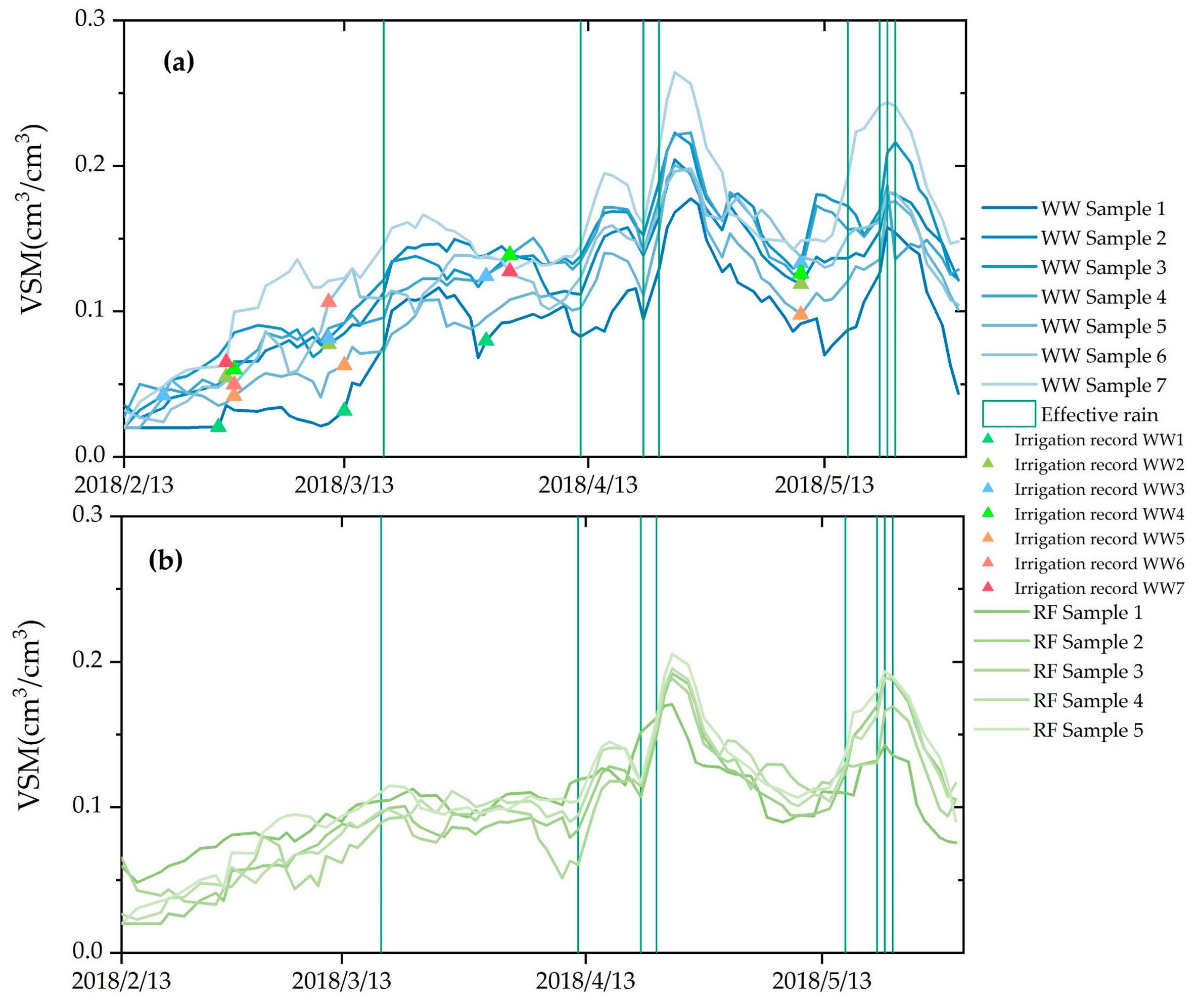
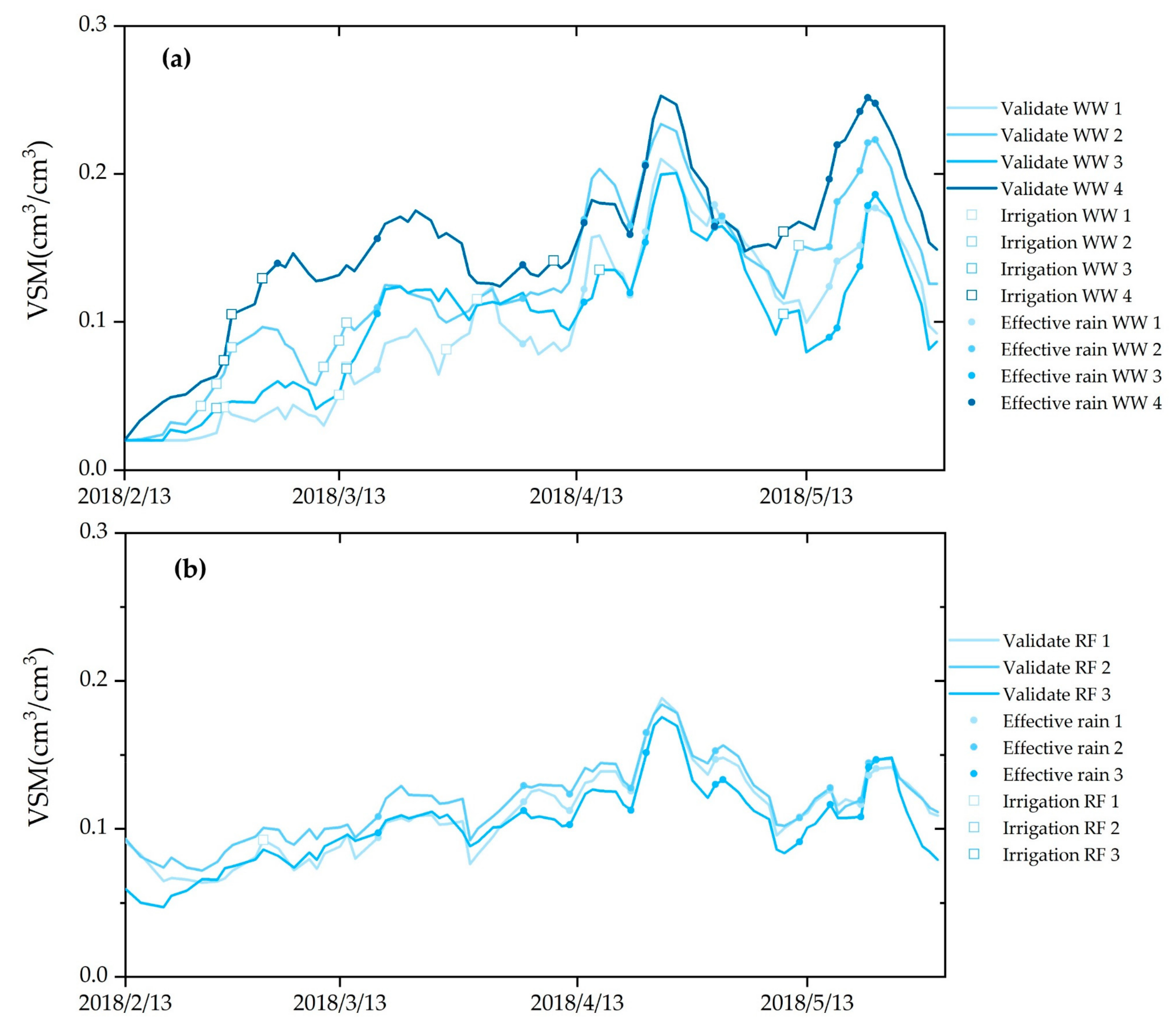
3.1.5. In Situ SM Measurement Data and Irrigation Records
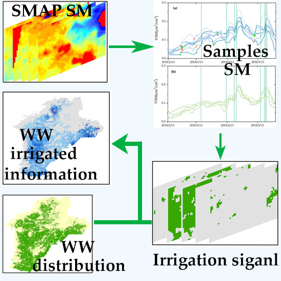
3.2. Methods
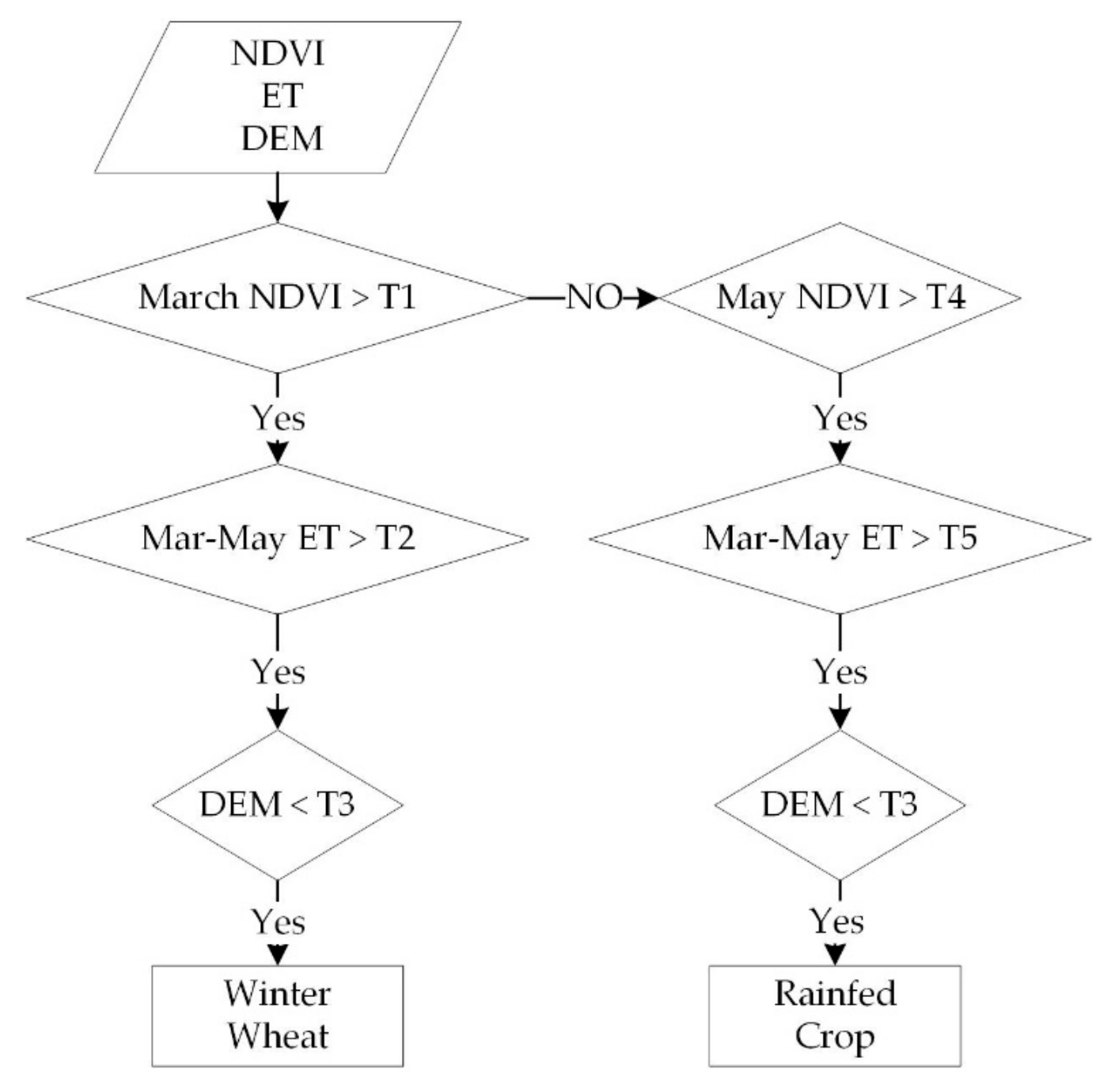
3.2.1. Established SMAP Training Samples for Winter Wheat and Rainfed Crops
3.2.2. Irrigation Information Detection and Irrigated Area Downscaling
3.2.3. Validation and Consistency Analysis
4. Results and Validation
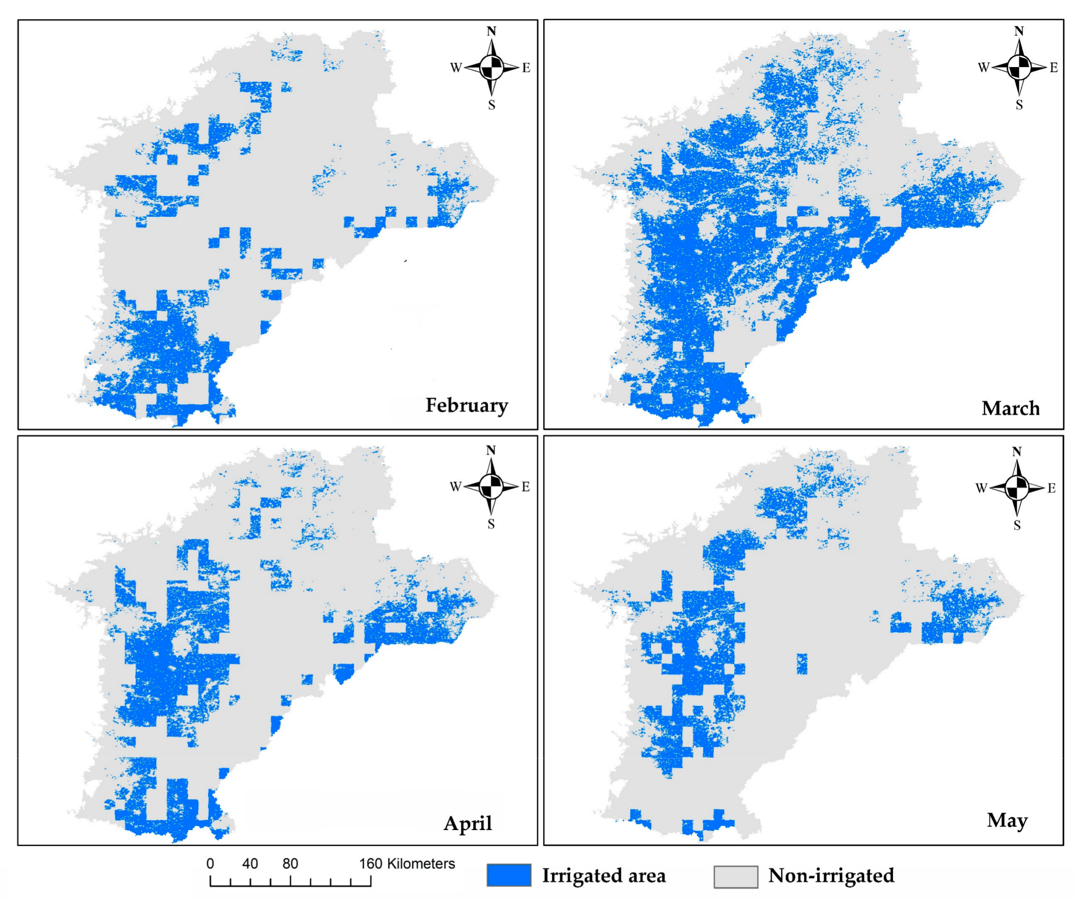
4.1. Irrigation Signal Detection
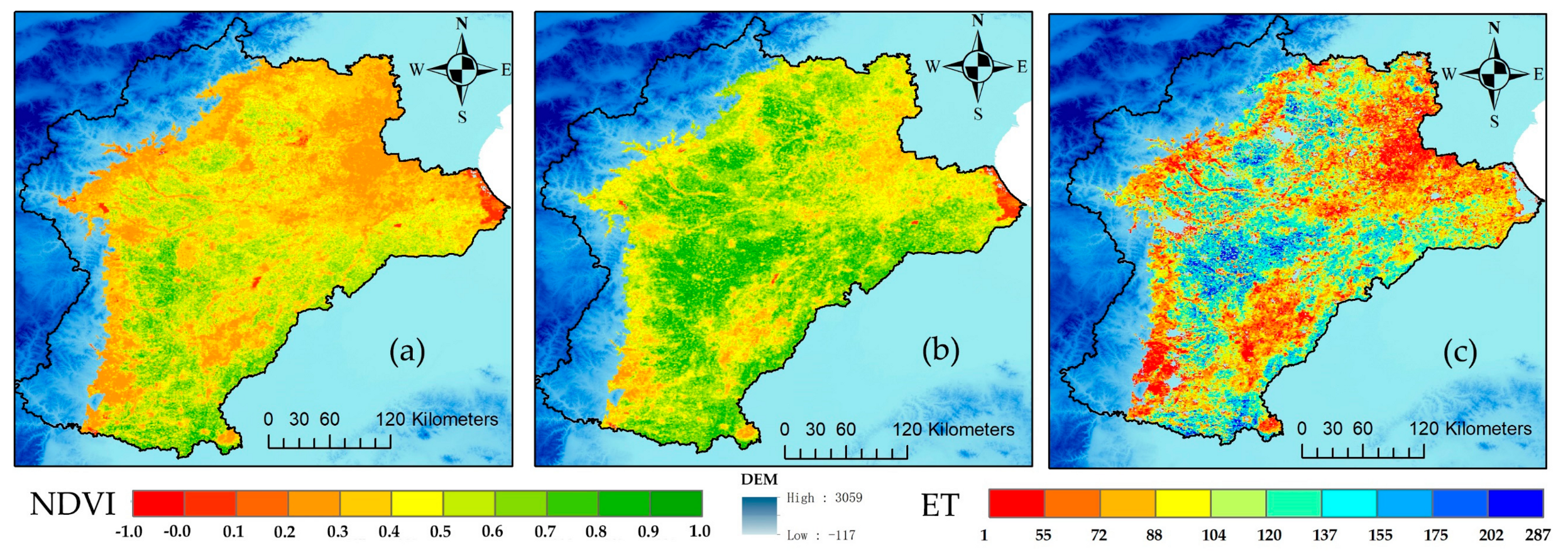
4.2. WW Extraction Results and Irrigated Area
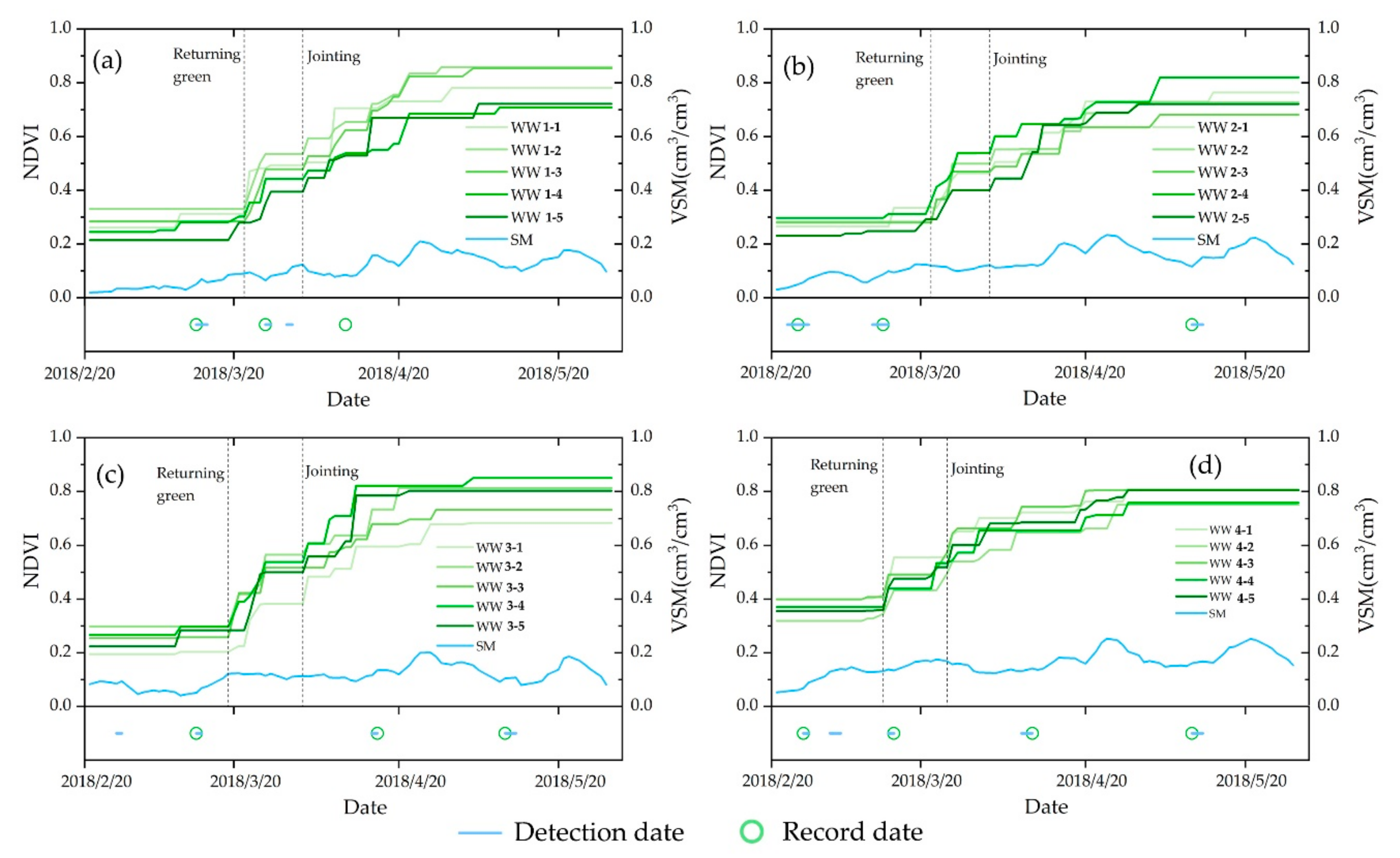
4.3. Validation and Growth Consistency Analysis
5. Discussion
5.1. Comparison with Other Studies
5.2. A Rational Discussion of the Irrigation Signal Detection Model
6. Conclusions
Author Contributions
Funding
Conflicts of Interest
References
- Li, J.; Inanaga, S.; Li, Z.; Eneji, A.E. Optimizing irrigation scheduling for winter wheat in the North China Plain. Agric. Water Manag. 2005, 76, 8–23. [Google Scholar] [CrossRef]
- Changming, L.; Jingjie, Y.; Kendy, E. Groundwater exploitation and its impact on the environment in the North China Plain. Water Int. 2001, 26, 265–271. [Google Scholar] [CrossRef]
- Min, Z.; Jianbin, D.; Houze, X.U.; Peng, P.; Haoming, Y.A.N.; Yaozhong, Z.H.U. Trend of China land water storage redistribution at medi- and large-spatial scales in recent five years by satellite gravity observations. Chin. Sci. Bull. 2009, 54, 816–821. [Google Scholar] [CrossRef]
- Feng, W.; Shum, C.K.; Zhong, M.; Pan, Y. Groundwater storage changes in China from satellite gravity: An overview. Remote Sens. 2018, 10, 674. [Google Scholar] [CrossRef]
- Xu, C.; Tao, H.; Tian, B.; Gao, Y.; Ren, J.; Wang, P. Field Crops Research Limited-irrigation improves water use efficiency and soil reservoir capacity through regulating root and canopy growth of winter wheat. Field Crop Res. 2016, 196, 268–275. [Google Scholar] [CrossRef]
- Wang, X.; Li, X. Irrigation Water Availability and Winter Wheat Abandonment in the North China Plain (NCP): Findings from a Case Study in Cangxian County of Hebei Province. Sustainability 2018, 10, 354. [Google Scholar] [CrossRef]
- Ali, M.H.; Hoque, M.R.; Hassan, A.A.; Khair, A. Effects of deficit irrigation on yield, water productivity, and economic returns of wheat. Agric. Water Manag. 2007, 92, 151–161. [Google Scholar] [CrossRef]
- Burney, J.; Woltering, L.; Burke, M.; Naylor, R.; Pasternak, D. Solar-powered drip irrigation enhances food security in the Sudano—Sahel. Proc. Natl. Acad. Sci. USA 2009, 10, 1848–1853. [Google Scholar] [CrossRef]
- Phogat, V.; Skewes, M.A.; Cox, J.W.; Sanderson, G.; Alam, J.; Šimůnek, J. Seasonal simulation of water, salinity and nitrate dynamics under drip irrigated mandarin (Citrus reticulata) and assessing management options for drainage and nitrate leaching. J. Hydrol. 2014, 513, 504–516. [Google Scholar] [CrossRef]
- Egea, G.; Diaz-espejo, A.; Fernández, J.E. Soil moisture dynamics in a hedgerow olive orchard under well-watered and deficit irrigation regimes: Assessment, prediction and scenario analysis. Agric. Water Manag. 2016, 164, 197–211. [Google Scholar] [CrossRef]
- Zhang, R.; Kim, S.; Sharma, A. Remote Sensing of Environment A comprehensive validation of the SMAP Enhanced Level-3 Soil Moisture product using ground measurements over varied climates and landscapes. Remote Sens. Environ. 2019, 223, 82–94. [Google Scholar] [CrossRef]
- Yi, Z.; Zhao, H.; Jiang, Y. Continuous Daily Evapotranspiration Estimation at the Field-Scale over Heterogeneous Agricultural Areas by Fusing ASTER and MODIS Data. Remote Sens. 2018, 10, 1694. [Google Scholar] [CrossRef]
- Yang, Y.; Tao, B.; Ren, W.; Zourarakis, D.P.; Masri, B.E.; Sun, Z.; Tian, Q. An Improved Approach Considering Intraclass Variability for Mapping Winter Wheat Using Multitemporal MODIS EVI Images. Remote Sens. 2019, 11, 1191. [Google Scholar] [CrossRef]
- Autovino, D.; Minacapilli, M.; Provenzano, G. Modelling bulk surface resistance by MODIS data and assessment of MOD16A2 evapotranspiration product in an irrigation district of Southern Italy. Agric. Water Manag. 2016, 167, 86–94. [Google Scholar] [CrossRef]
- Hao, Z.; Zhao, H.; Zhang, C.; Zhou, H.; Zhao, H.; Wang, H. Correlation Analysis Between Groundwater Decline Trend and Human-Induced Factors in Bashang Region. Water 2019, 11, 473. [Google Scholar] [CrossRef]
- Ozdogan, M.; Gutman, G. Remote Sensing of Environment A new methodology to map irrigated areas using multi-temporal MODIS and ancillary data: An application example in the continental US. Remote Sens. Environ. 2008, 112, 3520–3537. [Google Scholar] [CrossRef]
- Salmon, J.M.; Friedl, M.A.; Frolking, S.; Wisser, D.; Douglas, E.M. International Journal of Applied Earth Observation and Geoinformation Global rain-fed, irrigated, and paddy croplands: A new high resolution map derived from remote sensing, crop inventories and climate data. Int. J. Appl. Earth Obs. Geoinf. 2015, 38, 321–334. [Google Scholar] [CrossRef]
- Brown, J.F.; Pervez, S. Merging remote sensing data and national agricultural statistics to model change in irrigated agriculture. Agric. Syst. 2014, 127, 28–40. [Google Scholar] [CrossRef]
- Gumma, M.K. Mapping Irrigated Areas of Ghana Using Fusion of 30 m and 250 m Resolution Remote-Sensing Data. Remote Sens. 2011, 3, 816–835. [Google Scholar] [CrossRef]
- Pervez, S.; Budde, M.; Rowland, J. Remote Sensing of Environment Mapping irrigated areas in Afghanistan over the past decade using MODIS NDVI. Remote Sens. Environ. 2014, 149, 155–165. [Google Scholar] [CrossRef]
- Ambika, A.K.; Wardlow, B.; Mishra, V. Data Descriptor: Remotely sensed high resolution irrigated area mapping in India for 2000 to 2015. Nature 2016. [Google Scholar] [CrossRef]
- Pervez, S.; Brown, J.F. Data and National Agricultural Statistics. Remote Sens. 2010, 2, 2388–2412. [Google Scholar] [CrossRef]
- Chen, Y.; Lu, D.; Luo, L.; Pokhrel, Y.; Deb, K.; Huang, J.; Ran, Y. Detecting irrigation extent, frequency, and timing in a heterogeneous arid agricultural region using MODIS time series, Landsat imagery, and ancillary data. Remote Sens. Environ. 2018, 204, 197–211. [Google Scholar] [CrossRef]
- Xiao, X.; Boles, S.; Liu, J.; Zhuang, D.; Frolking, S.; Li, C.; Salas, W.; Moore, B. Mapping paddy rice agriculture in southern China using multi-temporal MODIS images. Remote Sens. Environ. 2005, 95, 480–492. [Google Scholar] [CrossRef]
- Peng, D.; Huete, A.R.; Huang, J.; Wang, F.; Sun, H. International Journal of Applied Earth Observation and Geoinformation Detection and estimation of mixed paddy rice cropping patterns with MODIS data. Int. J. Appl. Earth Obs. Geoinf. 2011, 13, 13–23. [Google Scholar] [CrossRef]
- Abuzar, M.; Mcallister, A.; Whitfield, D. Mapping Irrigated Farmlands Using Vegetation and Thermal Thresholds Derived from Landsat and ASTER Data in an Irrigation District of Australia. Photogramm. Eng. Remote Sens. 2015, 81, 229–238. [Google Scholar] [CrossRef]
- Liu, Y.Y.; Dorigo, W.A.; Parinussa, R.M.; de Jeu, R.A.; Wagner, W.; Mccabe, M.F.; Evans, J.P.; Dijk, A.I.J.M. Van Remote Sensing of Environment Trend-preserving blending of passive and active microwave soil moisture retrievals. Remote Sens. Environ. 2012, 123, 280–297. [Google Scholar] [CrossRef]
- Hutchinson, J.M.S. Estimating Near-Surface Soil Moisture using Active Microwave Satellite Imagery and Optical Sensor Inputs. Trans. ASAE 2003, 46, 225–236. [Google Scholar] [CrossRef]
- Pellarin, T.; Laurent, J. Soil moisture mapping over West Africa Soil moisture mapping over West Africa with a 30-min temporal resolution using AMSR-E observations and a satellite-based rainfall product. Hydrol. Earth Syst. Sci. 2010, 13, 1887–1896. [Google Scholar] [CrossRef]
- Colliander, A.; Jackson, T.J.; Bindlish, R.; Chan, S.; Das, N.; Kim, S.B.; Cosh, M.H.; Dunbar, R.S.; Dang, L.; Pashaian, L.; et al. Validation of SMAP surface soil moisture products with core validation sites. Remote Sens. Environ. 2017, 191, 215–231. [Google Scholar] [CrossRef]
- Chan, S.K.; Member, S.; Bindlish, R.; Neill, P.E.O.; Njoku, E.; Jackson, T.; Colliander, A.; Member, S.; Chen, F.; Burgin, M.; et al. Assessment of the SMAP Passive Soil Moisture Product. IEEE Trans. Geosci. Remote Sens. 2016, 54, 4994–5007. [Google Scholar] [CrossRef]
- Kumar, S.V.; Dirmeyer, P.A.; Peters-lidard, C.D.; Bindlish, R.; Bolten, J. Remote Sensing of Environment Information theoretic evaluation of satellite soil moisture retrievals. Remote Sens. Environ. 2017, 204, 392–400. [Google Scholar] [CrossRef]
- Lawston, P.M.; Joseph, A.; Santanello, J.A., Jr.; Sujay, V.K. Irrigation Signals Detected from SMAP Soil Moisture Retrievals. Geophys. Res. Lett. 2017, 44, 860–867. [Google Scholar] [CrossRef]
- Thenkabail, P.S.; Biradar, C.M. International Journal of Remote Global irrigated area map (GIAM), derived from remote sensing, for the end of the last millennium. Int. J. Remote Sens. 2009, 30, 3679–3733. [Google Scholar] [CrossRef]
- Wu, D.; Fang, S.; Li, X.; He, D.; Zhu, Y.; Yang, Z.; Xu, J. Spatial-temporal variation in irrigation water requirement for the winter wheat-summer maize rotation system since the 1980s on the North China Plain. Agric. Water Manag. 2019, 214, 78–86. [Google Scholar] [CrossRef]
- Zhao, Z.; Qin, X.; Wang, Z.; Wang, E. Agricultural and Forest Meteorology Performance of di ff erent cropping systems across precipitation gradient in North China Plain. Agric. For. Meteorol. 2018, 259, 162–172. [Google Scholar] [CrossRef]
- Zou, J.; Zhan, C.; Xie, Z.; Qin, P.; Jiang, S. Climatic impacts of the Middle Route of the South-to-North Water Transfer Project over the Haihe River basin in North China simulated by a regional climate model Jing. J. Geophys. Res. Atmos. 2016, 121, 8983–8999. [Google Scholar] [CrossRef]
- Entekhabi, D.; Yueh, S.; O’Neill, P.E.; Kellogg, K.H.; Allen, A.; Bindlish, R.; Brown, M.; Chan, S.; Colliander, A.; Crow, W.T. SMAP Handbook–Soil Moisture Active Passive: Mapping Soil Moisture and Freeze/Thaw from Space; JPL Publication: Pasadena, CA, USA, 2014. [Google Scholar]
- Pan, M.; Entekhabi, D.; Lu, H.; Akbar, R.; Peng, B.; McColl, K.A.; Short Gianotti, D.J.; Wang, W. Global characterization of surface soil moisture drydowns. Geophys. Res. Lett. 2017, 44, 3682–3690. [Google Scholar] [CrossRef]
- O’Neill, P.E.; Chan, S.; Njoku, E.G.; Jackson, T.; Bindlish, R. SMAP Enhanced L3 Radiometer Global Daily 9 Km EASE-Grid Soil Moisture, Version 1; NASA National Snow and Ice Data Center Distributed Active Archive Center: Boulder, CO, USA, 2016.
- Thenkabail, P.S.; Biradar, C.M.; Noojipady, P.; Dheeravath, V.; Li, Y.J.; Velpuri, M.; Reddy, G.P.O.; Cai, X.L.; Gumma, M.; Turral, H. A Global Irrigated Area Map (GIAM) Using Remote Sensing at The End of the Last Millennium; International Water Management Institute Colombo: Battaramulla, Sri Lanka, 2008; ISBN ISBN 9290906464. [Google Scholar]
- Ramankutty, N.; Huang, X.; Sulla-Menashe, D.; Friedl, M.A.; Sibley, A.; Tan, B.; Schneider, A. MODIS Collection 5 global land cover: Algorithm refinements and characterization of new datasets. Remote Sens. Environ. 2009, 114, 168–182. [Google Scholar] [CrossRef]
- Running, S.; Mu, Q.; Zhao, M. MOD16A2 MODIS/Terra Net Evapotranspiration 8-Day L4 Global 500m SIN Grid V006; NASA EOSDIS L. Process. DAAC: Sioux Falls, SD, USA, 2017.
- Vermote, E.; Wolfe, R. MOD09GA MODIS/Terra Surface Reflectance Daily L2G Global 1 km and 500 m SIN Grid V006; NASA EOSDIS L. Process. DAAC: Sioux Falls, SD, USA, 2015.
- Van Leeuwen, W.J.; Huete, A.R.; Laing, T.W. MODIS Vegetation Index Compositing Approach: A Prototype with AVHRR Data. Remote Sens. Environ. 1999, 280, 264–280. [Google Scholar] [CrossRef]
- Dwyer, J.; Schmidt, G. The MODIS Reprojection Tool. In Earth Science Satellite Remote Sensing; Springer: Berlin, Germany, 2006. [Google Scholar]
- Zhong, Y.; Zhong, M.; Feng, W.; Wu, D. Groundwater Depletion in the West Liaohe River Basin, China and Its Implications Revealed by GRACE and in Situ Measurements. Remote Sens. 2018, 10, 493. [Google Scholar] [CrossRef]
- Zhang, X.; Chen, S.; Sun, H.; Shao, L.; Wang, Y. Changes in evapotranspiration over irrigated winter wheat and maize in North China Plain over three decades. Agric. Water Manag. 2011, 98, 1097–1104. [Google Scholar] [CrossRef]
- Sun, H.; Shen, Y.; Yu, Q.; Flerchinger, G.N.; Zhang, Y.; Liu, C.; Zhang, X. Effect of precipitation change on water balance and WUE of the winter wheat-summer maize rotation in the North China Plain. Agric. Water Manag. 2010, 97, 1139–1145. [Google Scholar] [CrossRef]
- Chen, C.; Baethgen, W.E.; Wang, E.; Yu, Q. Characterizing spatial and temporal variability of crop yield caused by climate and irrigation in the North China Plain. Theor. Appl. Climatol. 2011, 106, 365–381. [Google Scholar] [CrossRef]
- Yang, Y.; Yang, Y.; Moiwo, J.P.; Hu, Y. Estimation of irrigation requirement for sustainable water resources reallocation in North China. Agric. Water Manag. 2010, 97, 1711–1721. [Google Scholar] [CrossRef]
- Velpuri, N.M.; Thenkabail, P.S.; Gumma, M.K.; Biradar, C.; Dheeravath, V.; Noojipady, P.; Yuanjie, L. Influence of resolution in irrigated area mapping and area estimation. Photogramm. Eng. Remote Sens. 2009, 75, 1383–1395. [Google Scholar] [CrossRef]
- Wang, J.; Gong, S.; Xu, D.; Yu, Y.; Zhao, Y. Impact of drip and level-basin irrigation on growth and yield of winter wheat in the North China Plain. Irrig. Sci. 2013, 31, 1025–1037. [Google Scholar] [CrossRef]
- Zia, S.; Wenyong, D.; Spreer, W.; Spohrer, K.; Xiongkui, H.; Müller, J. Assessing crop water stress of winter wheat by thermography under different irrigation regimes in North China Plain. Int. J. Agric. Biol. Eng. 2012, 5, 24–34. [Google Scholar] [CrossRef]


| Data Source | Temporal Resolution | Spatial Resolution | Time Period | Data Access |
|---|---|---|---|---|
| SMAP | daily | 9 km | March 2015 to December 2018 | https://nsidc.org/data/SPL3SMP_E/versions/2 |
| PRE | daily | site | March 2015 to December 2018 | http://data.cma.cn/ |
| MOD09GA | daily | 500 m | March 2015 to December 2018 | https://ladsweb.modaps.eosdis.nasa.gov/ |
| MOD16A2 | 8-day | 500 m | March 2015 to December 2018 | https://ladsweb.modaps.eosdis.nasa.gov/ |
| Irrigated Map | year | 1 km and 500 m | http://www.iwmi.cgiar.org/ https//dl.dropboxusercontent.com/u/12683052/GRIPCmap.zip | |
| Irrigation Records | 10-day | site | January 2018 to December 2018 |
| WW 1 | WW 2 | WW 3 | WW 4 | RF 1 | RF 2 | RF 3 | ||||||||
|---|---|---|---|---|---|---|---|---|---|---|---|---|---|---|
| Rec | Det | Rec | Det | Rec | Det | Rec | Det | Rec | Det | Rec | Det | Rec | Det | |
| Dates | 2/26 | 2/24 | 2/23 | 2/26 | 2/26 | 2/26 | / | 3/3 | / | / | / | / | ||
| 3/13 | 3/13 | 2/25 | 3/13 | 3/14 | 2/27 | / | / | / | / | / | / | |||
| 3/14 | 2/27 | 4/15 | 4/16 | 3/3 | / | / | / | / | / | / | ||||
| 3/26 | 3/27 | 3/12 | 3/12 | 5/10 | 5/10 | 3/14 | 3/14 | / | / | / | / | / | / | |
| 3/31 | 3/13 | 4/10 | 4/10 | / | / | / | / | / | / | |||||
| 4/10 | 3/14 | 5/10 | 5/10 | / | / | / | / | / | / | |||||
| 5/11 | 5/12 | / | / | / | / | / | / | |||||||
| Accuracy | 50.00% | 100.00% | 75.00% | 83.33% | ||||||||||
| Overall accuracy | 77.08% | |||||||||||||
| WW1 | WW2 | WW3 | WW4 | WW5 | WW6 | WW7 | WW8 | WW9 | WW10 | WW11 | |
|---|---|---|---|---|---|---|---|---|---|---|---|
| RG | 3 | 5 | 4 | 2 | 3 | 5 | 5 | 4 | 3 | 5 | 4 |
| J | 4 | 4 | 4 | 5 | 5 | 5 | 5 | 4 | 4 | 3 | 5 |
| P | 70.00% | 90.00% | 80.00% | 70.00% | 80.00% | 100.00% | 100.00% | 80.00% | 70.00% | 80.00% | 90.00% |
| OA | 82.72% | ||||||||||
© 2019 by the authors. Licensee MDPI, Basel, Switzerland. This article is an open access article distributed under the terms and conditions of the Creative Commons Attribution (CC BY) license (http://creativecommons.org/licenses/by/4.0/).
Share and Cite
Hao, Z.; Zhao, H.; Zhang, C.; Wang, H.; Jiang, Y. Detecting Winter Wheat Irrigation Signals Using SMAP Gridded Soil Moisture Data. Remote Sens. 2019, 11, 2390. https://doi.org/10.3390/rs11202390
Hao Z, Zhao H, Zhang C, Wang H, Jiang Y. Detecting Winter Wheat Irrigation Signals Using SMAP Gridded Soil Moisture Data. Remote Sensing. 2019; 11(20):2390. https://doi.org/10.3390/rs11202390
Chicago/Turabian StyleHao, Zhen, Hongli Zhao, Chi Zhang, Hao Wang, and Yunzhong Jiang. 2019. "Detecting Winter Wheat Irrigation Signals Using SMAP Gridded Soil Moisture Data" Remote Sensing 11, no. 20: 2390. https://doi.org/10.3390/rs11202390
APA StyleHao, Z., Zhao, H., Zhang, C., Wang, H., & Jiang, Y. (2019). Detecting Winter Wheat Irrigation Signals Using SMAP Gridded Soil Moisture Data. Remote Sensing, 11(20), 2390. https://doi.org/10.3390/rs11202390