Snow-Covered Area Retrieval from Himawari–8 AHI Imagery of the Tibetan Plateau

Abstract

Daily snow-covered area retrieval using the imagery in solar reflective bands often encounters extensive data gaps caused by cloud obscuration. With the inception of geostationary satellites carrying advanced multispectral imagers of high temporal resolution, such as Japan’s geostationary weather satellite Himawari–8, considerable progress can now be made towards spatially-complete estimation of daily snow-covered area. We developed a dynamic snow index (normalized difference snow index for vegetation-free background and normalized difference forest–snow index for vegetation background) fractional snow cover estimation method using Himawari–8 Advanced Himawari Imager (AHI) observations of the Tibetan Plateau. This method estimates fractional snow cover with the pixel-by-pixel linear relationship of snow index observations acquired under snow-free and snow-covered conditions. To achieve reliable snow-covered area mapping with minimal cloud contamination, the daily fractional snow cover can be represented as the composite of the high temporal resolution fractional snow cover estimates during daytime. The comparison against reference fractional snow cover data from Landsat–8 Operational Land Imager (OLI) showed that the root–mean–square error (RMSE) of the Himawari–8 AHI fractional snow cover ranged from 0.07 to 0.16, and that the coefficient of determination (R²) reached 0.81–0.96. Results from the 2015/2016 and 2016/2017 winters indicated that the daily composite of Himawari–8 observations obtained a 14% cloud percentage over the Tibetan Plateau, which was less than the cloud percentage (27%) from the combination of Moderate Resolution Imaging Spectroradiometer (MODIS) onboard Terra and Aqua.

1. Introduction

Snow cover, a spatially extensive and variable component of the Earth’s cryosphere, significantly affects the hydrologic cycle, weather, and climate. Water melted from seasonal snow cover provides essential water resources in middle- and high-latitude alpine areas [1,2]. In the Tibetan Plateau, snowmelt presents considerable contributions to the upstream areas of major Asian rivers [3,4,5]. In addition, snow is characterized by high albedo, low thermal conductivity, and considerable storage of latent heat of fusion and sublimation [6]. Thus, the accumulation and depletion of snow cover has a significant influence on the surface energy balance and the climate system [7,8]. Previous studies revealed that East Asian atmospheric circulation and the summer monsoon are largely influenced by the snow cover dynamics of the Tibetan Plateau [9,10,11,12,13].

The change of the snow-covered area (SCA) spatial distribution can be efficiently monitored using the time series of remote sensing imagery from space. Snow has a spectral signature distinguishable from most other land surface features in the visible and shortwave infrared spectrum [14,15]. From the understanding of snow’s spectral signature, the spatial distribution of snow-covered area can be estimated with observations at the solar reflective bands of multispectral imager onboard satellites, such as the Thematic Mapper (TM) onboard Landsat–5, Advanced Very High Resolution Radiometer (AVHRR) onboard National Oceanic and Atmospheric Administration (NOAA) satellites, and the Moderate Resolution Imaging Spectroradiometer (MODIS) onboard Terra and Aqua [14,16,17,18,19]. For multispectral images at fine spatial resolution, the normalized difference snow index (NDSI) is quite useful for binary snow cover estimation. However, snow cover is often patchy around the snowline and in the central Tibetan Plateau. To obtain a reliable snow-covered area at a relatively coarse resolution, the estimation of the areal fraction of snow within each pixel (fractional snow cover, FSC) is necessary. Among the widely used fractional snow cover products, the MODIS daily snow cover products, including NASA’s MOD10 suite and MODIS Snow-Covered Area and Grain size (MODSCAG), are reported to be highly accurate and to satisfy the balance between spatial resolution and revisit period [20,21,22,23].

Due to cloud obscuration at visible and infrared observations of land surface, however, the MODIS daily snow-covered area maps often encounter data gaps. To address the spatio–temporal continuity of MODIS snow-covered area estimation, data-filling approaches with spatial and temporal neighboring information can be utilized. The cloud-gap-filled algorithm and the time-domain filtering method use the clear-sky observations on previous days to represent the Terra MODIS’s snow-covered area on the current cloudy day [24,25]. The spatio–temporal filtering on the combination of Terra and Aqua MODIS is also well accepted to complete the daily MODIS snow-covered area [26,27]. Some ancillary information, including surface temperature, elevation, and sensor zenith angle, can contribute to the reduction of uncertainties in the cloud-free snow-covered area data [28,29,30,31,32].

Another feasible solution for cloud removal in daily snow-covered area mapping is to acquire frequent observations within a single day and use the temporal compositing technique to remove non–persistent clouds. Geostationary weather satellites can provide frequent multispectral observations over a large area of about one-third of the Earth’s surface. The Geostationary Operational Environmental Satellite (GOES) series has enabled automated snow cover mapping over North America for a long time [33,34,35], while the Meteosat Second Generation (MSG) works for snow cover monitoring over Europe [36,37]. For observations of East Asia, the FengYun–2 (FY–2) geostationary weather satellite series has been used in not only binary snow cover mapping based on a classification strategy but also fractional snow cover estimation based on two–endmember linear spectral mixture analysis of the visible band [38,39]. However, the relatively coarse spatial resolution and the limitation of band designations of FY–2 can produce non-negligible uncertainties for snow-covered area retrieval.

Given the launch and operation of new advanced geostationary weather satellites such as Himawari–8 and FengYun-4A (FY–4A), the snow-covered area mapping over China has become more reliable and closer to real time. Himawari–8 was successfully launched on 7 October 2014 and has been operational since 7 July 2015. The Advanced Himawari Imager (AHI) onboard Himawari–8 is a multispectral imager and completes full-disk scanning at 10 min intervals [40]. In this study, we developed a framework to retrieve the snow-covered area from Himawari–8 AHI imagery of the Tibetan Plateau. Specifically, we first investigated and interpreted the relationship between NDSI/normalized difference forest–snow index (NDFSI) and fractional snow cover according to land cover type. Secondly, we implemented the dynamic snow index method for Himawari–8 AHI imagery and conducted the daily composite of the high temporal Himawari–8 fractional snow cover. Finally, this framework’s performance on the snow-covered area estimation and cloud removal effectiveness was illustrated. Such a daily snow-covered area estimation framework designed for Himawari–8, which is also possibly feasible for FY–4A, can make accurate and nearly cloud-free daily snow-covered area data at the relatively high spatial resolution available for applications in hydrological and climate research.

2. Study Region and Data Sources

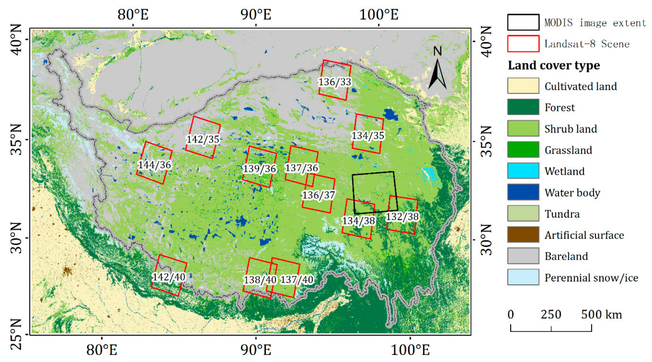
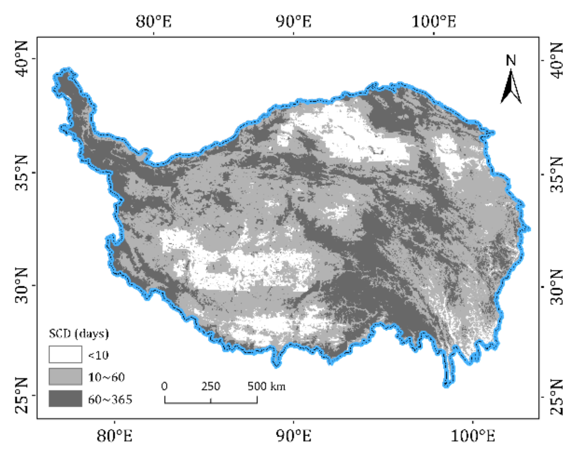
2.1. Study Region

The Tibetan Plateau, also referred to as the Third Pole, is generally characterized as the highest and most extensive plateau on the Earth [41]. With a geographical range of roughly 26°–40°N and 73°–105°E [42], the Tibetan Plateau encompasses a cold and dry environment. Due to precipitation reduction from southeast to northwest, vegetation on the plateau varies from a small area of broad-leaf and coniferous forests to expansive alpine meadows and steppes, whereas bare lands span predominantly across the northwest [43,44]. Figure 1 shows that the Tibetan Plateau is covered by vast grasslands, most of which in the snow season, however, become withered and difficult to spectrally distinguish from barren land.

The Tibetan Plateau is among the three largest stable snow cover regions of China [45]; about 34% of the area has a snow cover duration longer than two months (shown in Figure 2). Glaciers and perennial snow cover prominently cap the mountains surrounding or traversing the plateau, such as the Himalayas, the Karakoram Mountains, the Kunlun Mountains, and the Qilian Mountains. The vast interior of the Tibetan Plateau has a predominantly continental snow regime, with maritime snow in the southeast. Patchy and optically thin snow [46] over the highly reflective barren lands, most of which are exposed rock and sand, presents difficulties in the extraction of snow information. Snow in the interior also has a short duration, partly due to sublimation driven by high wind speeds, dry air, and strong solar radiation.

2.2. Himawari–8 Advanced Himiwari Imager (AHI) Data

The Himawari–8 AHI has spectral and spatial characteristics (shown in

Table 1. Himawari–8 Advanced Himawari Imager (AHI) characteristics.

Band Number	Wavelength (μm)	Central Wavelength (μm)	Spatial Resolution (km)
1	0.45–0.49	0.46	1
2	0.50–0.53	0.51	1
3	0.60–0.68	0.64	0.5
4	0.84–0.87	0.86	1
5	1.59–1.63	1.6	2
6	2.24–2.28	2.3	2
7	3.78–3.99	3.9	2
8	5.83–6.65	6.2	2
9	6.74–7.14	7.0	2
10	7.25–7.44	7.3	2
11	8.40–8.78	8.6	2
12	9.45–9.82	9.6	2
13	10.2–10.6	10.4	2
14	10.9–11.6	11.2	2
15	11.9–12.9	12.3	2
16	13–13.6	13.3	2

) that are useful for discriminating between snow and clouds, as well as soil/rock, vegetation, and water bodies. Himawari–8 AHI observations are an important data source for snow–covered area mapping of the Tibetan Plateau, in particular before the operation of FY–4A AGRI.

The Japan Meteorological Agency operates Himawari–8 and publishes Himawari Standard Data in the Himawari Standard Format and Himawari L1 Gridded Data in NetCDF format (ftp://ftp.ptree.jaxa.jp/) [48]. The full-disk AHI imagery from Himawari L1 Gridded Data is projected in the equirectangular projection (in other words, the plate carrée projection or geographic projection) with a grid size of 0.02° and 0.05°. Along with sun–target–satellite geometry information, top-of-atmosphere (TOA) reflectance of solar bands and brightness temperature of mid- and long-wavelength infrared bands are within 60°S–60°N and 80°E–160°W. TOA reflectance with a grid size of 0.02° was employed in this study. We also obtained the Himawari–8 Level 2 Cloud Property product at 4 km spatial resolution [49] to mask clouds within the AHI imagery. Note that a small western part of the Tibetan Plateau has longitudes less than 80°E and that Himawari–8 AHI observations of that part are not archived in Himawari L1 Gridded Data, but in Himawari Standard Data. A user can acquire Himawari–8’s Himawari Standard Data within the last one month.

2.3. Landsat–8 Operational Land Imager (OLI) Data

As the in situ measurement of snow-covered area is highly limited due to human labor, in particular in the form of fractional snow cover, the snow-covered area carefully derived from high-resolution imagery is a good source of reference data. Landsat–8 was successfully launched on 11 February 2013 by NASA. The OLI onboard Landsat–8 observes the reflected radiance at visible, near-infrared, and shortwave infrared wavelengths at the spatial resolution of 30 m (shown in

Table 2. Landsat–8 Operational Land Imager (OLI) characteristics [52].

Band Number	Wavelength (μm)	Central Wavelength (μm)	Spatial Resolution (m)
1	0.44–0.45	0.44	30
2	0.45–0.51	0.48	30
3	0.53–0.59	0.56	30
4	0.64–0.67	0.66	30
5	0.85–0.88	0.87	30
6	1.57–1.66	1.6	30
7	2.11–2.29	2.2	30
8	0.50–0.68	0.59	30
9	1.36–1.38	1.37	30

). Due to the abundant spectral information at the fine spatial resolution of 30 m, Landsat–8 OLI can be used to map snow cover reliably based on atmospherically corrected reflectance of the Earth’s surface. We acquired the Landsat–8 OLI Surface Reflectance product distributed by the Earth Resources Observation and Science (EROS) Center of the U.S. Geological Survey (USGS) at https://Earthexplorer.usgs.gov.

Seasonal snow cover on the Tibetan Plateau is predominately thin and patchy snow, so even a spatial resolution of 30 m may encounter a mixture of snow and other surface features within a single pixel. In order to obtain reliable reference data, the Landsat–8 OLI snow-covered area maps were generated based on multiple endmember spectral mixture analysis (MESMA) for surface reflectances at OLI bands 1 through 7. The snow, vegetation, and soil endmembers can be extracted from Landsat–8 OLI scenes based on empirical criteria.

After the screening of clouds and water bodies, if they exist in the Landsat–8 OLI scenes, the fractional snow cover was estimated by a MESMA scheme enhanced for computational efficiency. The optimal endmembers were automatically selected from the current multispectral image using rigorous criteria [50]. To evaluate the Landsat–8 OLI fractional snow cover based on MESMA, a previous study used Chinese Gaofen–2 imagery at the spatial resolution of 3.2 m over the Tibetan Plateau and took into account three kinds of land cover types: forest, grass, and bare soil [51]. The evaluation results of that study showed that the overall accuracy of the Landsat–8 OLI fractional snow cover is about 0.95, and the root–mean–square error (RMSE) is lower than 0.1. Therefore, the Landsat–8 OLI fractional snow cover can be taken as reference to validate the snow-covered area data at medium spatial resolution.

2.4. Terra Moderate Resolution Imaging Spectroradiometer (MODIS) Data

NASA’s MODIS snow cover product (MOD10 suite) has been extensively used in hydrological models [53,54,55], land surface models [56,57], and snow cover variability studies [26,27,58]. The MOD10A1 Collection 6 is the recently released Terra MODIS snow cover product at a 500 m resolution (https://n5eil01u.ecs.nsidc.org), in which the fractional snow cover can be obtained by employing NDSI (defined in Equation (1)) data and the empirical retrieval approach presented in Equation (2) [59,60]. This empirical linear relationship for estimating fractional snow cover is equivalent to the linear interpolation between fixed NDSI values of pure snow and snow-free ground, which are approximately 0.6950 and 0.0069.

$$\mathrm{NDSI}=\frac{{\mathrm{R}}_{0.5\mathsf{\mu }\mathrm{m}}-{\mathrm{R}}_{1.6\mathsf{\mu }\mathrm{m}}}{{\mathrm{R}}_{0.5\mathsf{\mu }\mathrm{m}}+{\mathrm{R}}_{1.6\mathsf{\mu }\mathrm{m}}}$$

(1)

where R_0.5µm and R_1.6µm represent the reflectances at the 0.5 and 1.6 µm bands, respectively.

$$\mathrm{FSC}=1.4533\times \mathrm{NDSI}-0.0100=\frac{\mathrm{NDSI}-0.0069}{0.6950-0.0069}$$

(2)

where NDSI ranges from 0 to 1 (0%~100%), and fractional snow cover values would be truncated to this range as well.

In addition to the Landsat–8 OLI snow-covered area data taken as the reference data, we also used the MOD10A1 fractional snow cover for comparison with Himawari–8 AHI fractional snow cover. This was done to demonstrate the Himawari–8 AHI fractional snow cover mapping performance against the simple linear NDSI fractional snow cover approach.

2.5. Auxiliary Data

For the development and evaluation of snow-covered area retrieval methodology, we utilized auxiliary information, including the elevation and the land cover type of the Tibetan Plateau and a spectral library of snow, vegetation, soil, and water.

The elevation information used in this study was represented by the ETOPO1 1 Arc-Minute Global Relief Model (http://www.ngdc.noaa.gov/mgg/global/global.html) [61]. The selection of Landsat–8 OLI data and the analysis of topographic effects on fractional snow cover estimation (presented in Section 4) relied on the ETOPO digital elevation model (DEM) data. The land cover data in this study was labeled using the 30 m Global Land Cover Dataset (GlobeLand30) (http://www.globallandcover.com) [62]. We also used the spectral reflectance data of snow, vegetation, soil, and water from the Johns Hopkins University spectral library (http://speclib.jpl.nasa.gov) [63].

3. Methodology

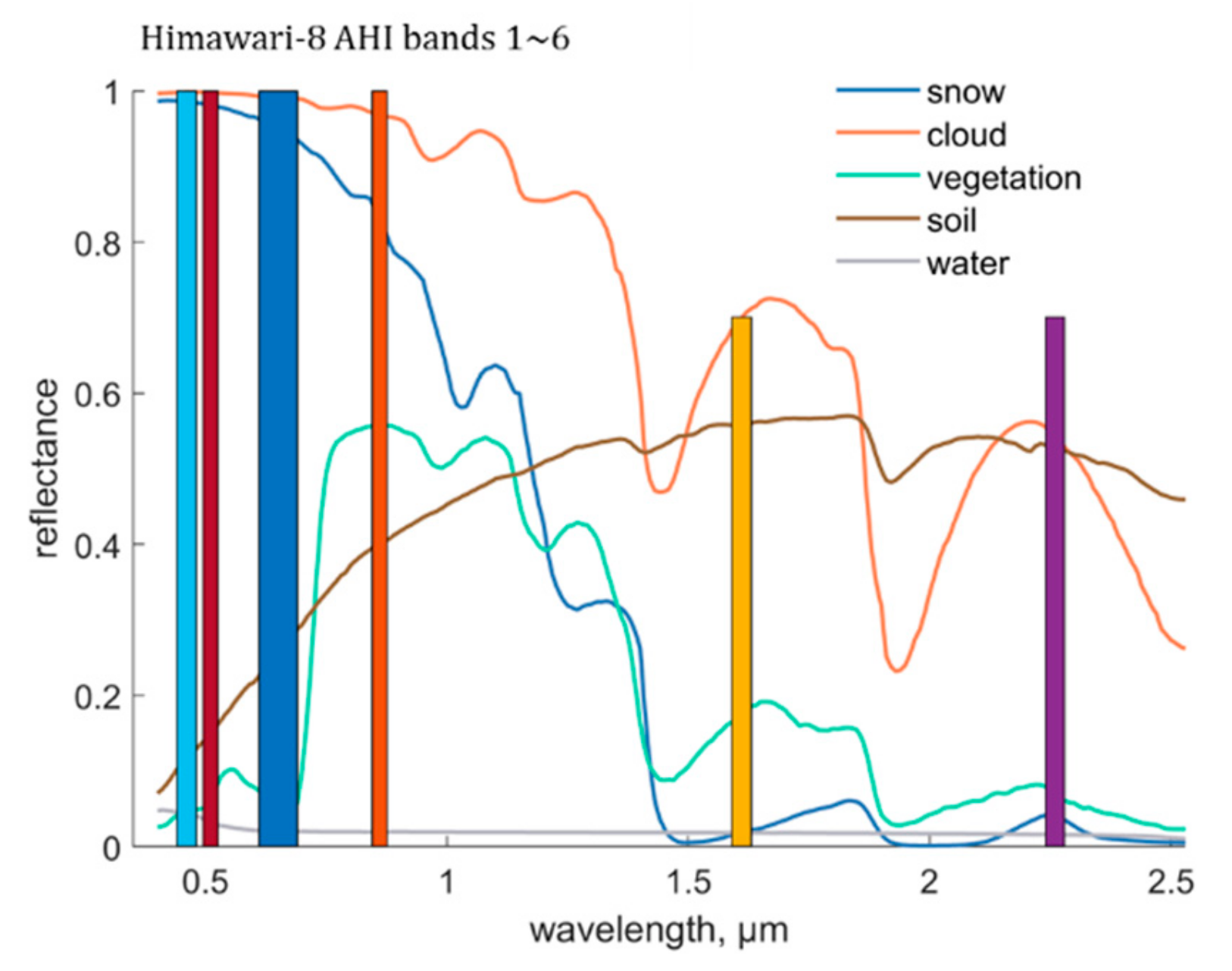
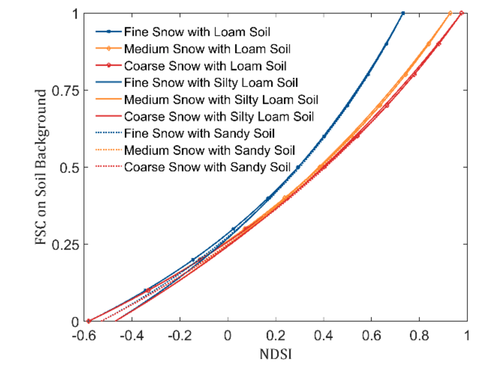
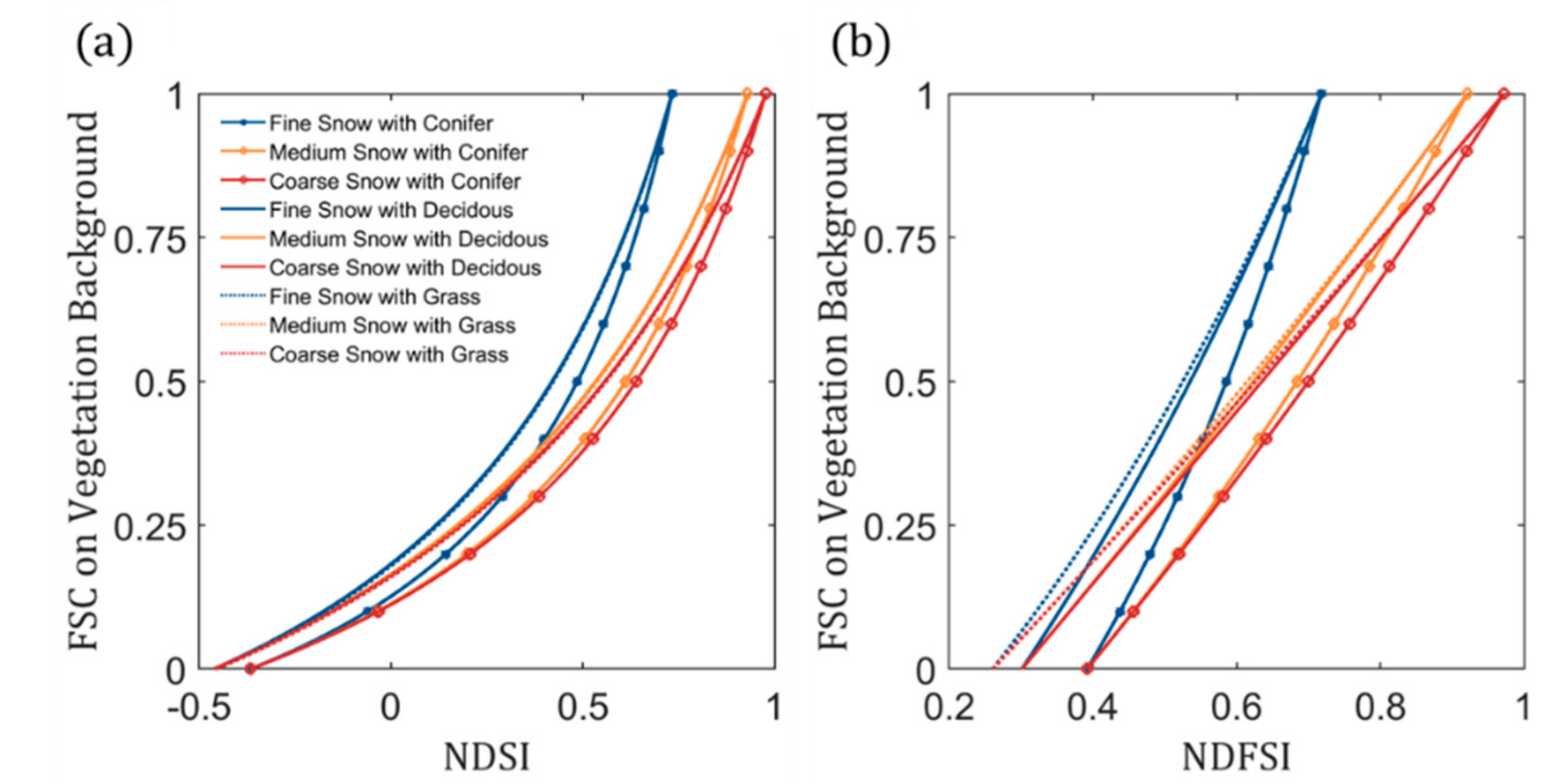
3.1. Indicating Fractional Snow Cover with Snow Indices

The reflectances of snow, water clouds, vegetation, and soil are shown in Figure 3, wherein the spectral ranges of Himawari–8 bands are also labeled. Clean snow is bright and white at visible wavelengths and clearly distinct from water bodies, vegetation, and soils. At shortwave infrared wavelengths, snow tends to have much lower reflectance due to the larger grain sizes than water clouds and some ice clouds. Through the interpretation of these snow reflective properties at visible and shortwave wavelengths, NDSI was taken as an effective factor to distinguish snow from other surface features and clouds [14]. In forested regions, NDFSI can be used to separate snow and snow-free forests [64]. NDFSI is expressed as follows:

$$\mathrm{NDFSI}=\frac{{\mathrm{R}}_{0.86\mathsf{\mu }\mathrm{m}}-{\mathrm{R}}_{1.6\mathsf{\mu }\mathrm{m}}}{{\mathrm{R}}_{0.86\mathsf{\mu }\mathrm{m}}+{\mathrm{R}}_{1.6\mathsf{\mu }\mathrm{m}}}$$

(3)

where R_0.86µm and R_1.6µm represent the reflectance at bands with wavelength centers of about 0.86 and 1.6 µm, respectively.

Highlighting snow’s spectral signature, high NDSI values can be used to determine the existence of snow in multispectral images, out of which clouds, water bodies, and shadows are screened. The values of NDSI can also indicate fractional snow cover, and the well-known MODIS snow cover product MOD10 suite is based on the empirical linear relationship between NDSI and fractional snow cover [60,65]. However, the static relationship may lead to considerable errors in global applications because NDSI varies not only with fractional snow cover but also with land cover types and sun–target–sensor geometry, which are highly variable in Himawari–8 AHI imagery.

To explore the NDSI dependence of fractional snow cover and the spectral characteristics of snow and snow-free ground, we generated NDSI values from the linear mixture of snow and non-snow features, with fractional snow cover ranging from 0% to 100%. The reflectance of snow, soil, and vegetation from the Johns Hopkins University Spectral Library was used in the simulation of NDSI and NDFSI. To note, bidirectional properties of snow and non-snow features were not taken into account. In the simulation, we employed the single scattering approximation and assumed that a mixed pixel consists of a single type of snow and only one type of non-snow feature and that snowpack is deep enough to obstruct the optical signal from underlying ground. Then the reflectance of a mixed pixel is determined by a linear sum of the reflectances of a type of snow and a non-snow feature. Once that reflectance is calculated for all the bands required by NDSI and NDFSI, the relationship between snow’s area fraction (the weight in the contribution to a mixed pixel) and NDSI/NDFSI with respect to land cover type can be simulated.

Figure 4 shows the relationship between NDSI and snow’s area fraction (fractional snow cover) for pure, optically thick snow of fine, medium, and coarse grain sizes mixed with three types of soils. The slightly curved relationships shown in Figure 4 indicate that the relationship between fractional snow cover and NDSI approximates a linear function in the condition of soil background. We took the NDSI values of soil background (snow-free) and pure snow and then the linear relationship between fractional snow cover and NDSI was made for various types of soil and snow. Based on these linear relationships, the RMSE of fractional snow cover estimation was found to be within the range of 0.07–0.13 compared with the nonlinear relationships shown in Figure 4.

For vegetation background, however, NDSI does not vary linearly with fractional snow cover according to modeling results shown in Figure 5a. This is because, unlike soil, vegetation’s reflectance at the green band is much lower, and at the 1.6 µm band, slightly higher than snow. Employing the 0.86 µm band rather than the green band, the differences of snow’s and vegetation’s reflectances at the two bands used in NDSI calculation can be balanced. Consequently, the relationship between fractional snow cover and NDFSI is close to a linear function as shown in Figure 5b.

3.2. Estimating Fractional Snow Cover with Local Dynamic Snow Indices

For snow cover mapping of rugged areas with an enormous number of observations in terms of high temporal resolution of Himawari–8 AHI, relying on NDSI to estimate fractional snow cover is a simple and feasible method. Moreover, NDSI can perform well even with the absence of precise atmospheric and topographic correction [60]. Based on the linear assumption discussed in Section 3.1, fractional snow cover retrieval with NDSI and NDFSI can be applied using Equations (4) and (5) for pixels having NDSI/NDFSI higher than the background that determined by the composite of prior snow-free observations. Figure 4 and Figure 5b indicate that this linear assumption can result in fractional snow cover errors having values of 0.07–0.13 for soil background and < 0.10 for vegetation background, with variation of snow grain size taken into consideration.

$$\mathrm{FSC}=\frac{\mathrm{NDSI}-{\mathrm{NDSI}}_{\mathrm{soil}}}{{\mathrm{NDSI}}_{\mathrm{snow}}-{\mathrm{NDSI}}_{\mathrm{soil}}} \left(\mathrm{soil} \mathrm{background}\right)$$

(4)

$$\mathrm{FSC}=\frac{\mathrm{NDFSI}-{\mathrm{NDFSI}}_{\mathrm{veg}}}{{\mathrm{NDFSI}}_{\mathrm{snow}}-{\mathrm{NDFSI}}_{\mathrm{veg}}} \left(\mathrm{vegetation} \mathrm{background}\right)$$

(5)

where NDSI_snow and NDSI_soil are the NDSI values for pure snow and soil, respectively, and NDFSI_snow and NDFSI_veg are the NDFSI values for pure snow and vegetation, respectively. The vegetation background is determined if the normalized difference vegetation index (NDVI) of the background map is higher than 0.3.

To calculate fractional snow cover for each scene generated at different daytimes, NDSI_soil and NDFSI_veg were obtained from the clear-sky snow-free observations on the most recent day. NDSI_snow can be modeled or selected from multispectral images. Observed NDSI/NDFSI above NDSI_snow/NDFSI_snow was considered to have a fractional snow cover value of 100%, and similarly, NDSI/NDFSI below NDSI_soil/NDFSI_veg was considered to be snow-free. The NDSI of pure snow depends on snow grain size and sun–target–sensor geometry. To examine the effects of snow grain size and solar zenith angle on NDSI, we modeled the directional-hemispherical reflectance of snow. First, we calculated the single scattering properties from Mie scattering theory with spherical snow particle assumption used. Mie calculations for spherical particles can mimic the scattering properties of snow because irregularly shaped snow particles are often not oriented [14]. Given the resulting scattering properties as input, a two-stream radiative transfer model was used to calculate the directional-hemispherical reflectance of snow. A very high NDSI value of snow could be associated with large grain size and/or small solar zenith angle. For a solar zenith angle ranging from 25° to 60°, modeling results of clean snow with a grain size larger than 500 µm showed that the NDSI values are nearly 1.0. Viewing zenith angle influences NDSI as well. As clean snow has a strong anisotropy in near infrared and shortwave infrared wavelengths [66,67], snow’s reflectance at 0.86 μm can range from about 0.85 to 1.0 for the viewing zenith angle varying from 0° to 60° [68], and that at 1.6 μm can increase from 0.02 to 0.20 for the viewing zenith angle varying from 0° to 80° [69]. However, fresh snow is approximately Lambertian with an average reflectance close to 1.0 [68]. Therefore, a rough range of NDSI values taken the variety of viewing zenith angle into account can be calculated, and the result is [0.67, 0.96]. For NDFSI, that range is from 0.62 to 0.96. Himawari–8 AHI observations indicate that the NDSI of the glaciers in the Himalaya region is generally nearly equal to or higher than 0.7. Note that the MOD10 algorithm (see Equation (2)) takes a value of about 0.70 as the NDSI threshold of pure snow cover; hence, we chose a conservative value of 0.70 for NDSI_snow in the retrieval procedure.

As shown in Figure 5, though the curves of fractional snow cover dependent on NDSI for the vegetation background are apparently far away from linear functions, fractional snow cover varies with NDFSI near linearly. With the introduction of NDFSI, the fractional snow cover for vegetation areas was taken as a linear function of NDFSI observations of pure snow and snow-free land. The NDFSI_snow is represented here by an empirical and constant value of 0.70.

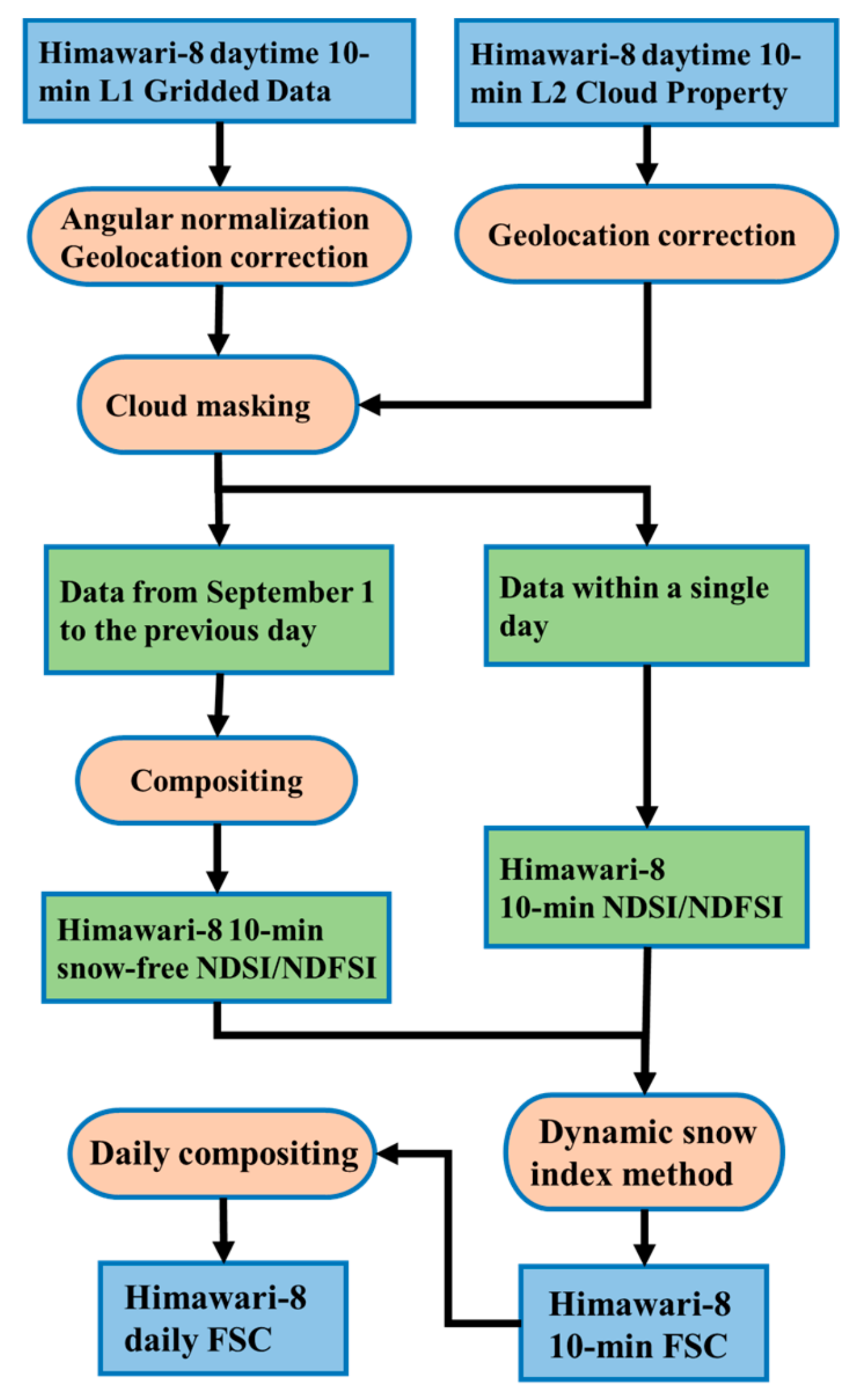
3.3. Himawari–8 Data Preprocessing

A flowchart describing the fractional snow cover retrieval process of Himawari–8 AHI data is shown in Figure 6. The data preprocessing consisted of three major steps: angular normalization, geolocation correction, and cloud masking.

Angular normalization is necessary because of the reflectance’s variability at different sensor/sun zenith angles. The optical imagery from geostationary weather satellites is characterized by the spatial variability of the sensor zenith angle and the spatiotemporal variability of the solar zenith angle. Then, reflectance fluctuates at non-Lambertian surfaces due to the change of sun–target–sensor geometry throughout the daytime and the full-disk image.

The reflectance’s variability was reduced using a bidirectional reflectance model for the angular effect correction [70]. This model is a semiempirical kernel-driven model consisting of a volumetric scattering kernel, a geometric-optical kernel, and two corresponding coefficients as well as a constant. The coefficient of determination (R²) of this bidirectional reflectance model compared with in situ observations can reach 0.51–0.91 [70]. The model parameters were determined by regression and then the reflectance data was corrected to a reference illuminating-viewing geometry condition, that is, 60° for the solar zenith angle, 65° the satellite zenith angle, and 35° the relative azimuth angle, which is roughly consistent with the condition of Himawari–8’s viewing of the central plateau at midday in January. The geolocation of Himawari–8 AHI imagery has errors under off-nadir viewing conditions, so we also corrected the geolocation errors at the Tibetan Plateau with the ground control points selected at the edge of the lakes on the Tibetan Plateau. The georeferencing resulted in a mean absolute error of about 0.7 pixels in the west–east direction and about 0.5 pixels in the north–south direction according to the evaluation using independent ground control points.

Prior to the snow-covered area mapping, clouds should be screening out from the multiple spectral images because some clouds, including ice clouds and cirrus, are very similar to snow in solar reflective bands and are likely to result in erroneous snow identification. In this study, we employed the cloud mask information packed in the Quality Assurance (QA) layer of the Himawari–8 Level 2 Cloud Property product to determine cloud-contaminated pixels.

3.4. Himawari–8 Snow-Covered Area Retrieval

The dynamic snow index approach to retrieve the snow-covered area relying on the near-linear relationship between fractional snow cover and NDSI/NDFSI was first implemented for each instantaneous image of Himawari–8 AHI. Then, instantaneous fractional snow cover estimates within a single day were composited to remove data gaps mainly caused by clouds. The present approach for mapping of the snow-covered area was based on the daytime observations between UTC 2:00 and 9:00 a.m. (i.e., roughly from 7:00 to 16:00 in the local time of the Tibetan Plateau). The solar zenith angle was limited to < 75° in the processing. NDSI_soil and NDFSI_veg were determined by the snow-free observation of the moment on the most recent day. In other words, the pixel-by-pixel NDSI_soil and NDFSI_veg may vary throughout the time within a single day. In practice, the “background map” towards the absence of clouds, shadows, and snow for calculating NDSI_soil and NDFSI_veg was generated by compositing observations from September 1 to the previous day, wherein the priority comes to a lower NDSI except for water bodies determined from the land cover map. The final background map could not ultimately be snow-free (typically, NDSI < 0) in regions of glaciers and perennial snow cover, for which the NDSI_soil and NDFSI_veg were obtained from the nearest neighbor pixels. Additionally, to reduce the spurious snow-covered area caused by noisy changes of the snow index value, we excluded fractional snow cover that was lower than 0.2 with the band 5 reflectance of higher than 0.2.

With the high resolution observations in a single day, the generation of the daily snow-covered area is dependent on the temporal compositing technique. The principle of the daily composite of snow-covered area is eliminating the cloud obscuration and enhancing the reliability of snow cover retrieval. The basic strategy for temporal compositing is blending cloudless snow-covered area retrievals. However, there may be many alternative clear-sky observations and the uncertainty within them is subtle. We selected the clear-sky fractional snow cover under the smallest solar zenith angle to represent the daily estimate. A higher solar height generally results in warmer surface temperatures and smaller shaded areas due to cloud cover and rugged terrain. Snow cover enduring illumination under a high solar height condition is likely to persist for a whole day. Therefore, spurious identification of snow can be potentially removed.

3.5. Evaluation Metrics

Selected metrics for validation of Himawari–8 AHI snow-covered area included the overall accuracy, precision, recall, RMSE, and R², which are defined below:

$$\mathrm{Overall} \mathrm{accuracy}=\frac{TP+TN}{TP+TN+FP+FN}$$

(6)

$$\mathrm{Precision}=\frac{TP}{TP+FP}$$

(7)

$$\mathrm{Recall}=\frac{TP}{TP+FN}$$

(8)

$$\mathrm{RMSE}=\sqrt{\frac{1}{N}{\displaystyle \sum }_N{\left(f_{est}-f_{ref}\right)}^2}$$

(9)

$$R^2=\frac{{\left[\sum \left(f_{est}-\overline{f_{est}}\right)\left(f_{ref}-\overline{f_{ref}}\right)\right]}^2}{\sum {\left(f_{est}-\overline{f_{ref}}\right)}^2·\sum {\left(f_{ref}-\overline{f_{ref}}\right)}^2}$$

(10)

where TP indicates true positive, TN indicates true negative, FP indicates false positive, FN indicates false negative, f_est indicates fractional snow cover estimation derived from Himawari–8 AHI, and similarly, f_ref indicates reference fractional snow cover derived from Landsat–8 OLI. To calculate overall accuracy, snow cover was labeled for pixels with fractional snow cover ≥ 0.15 [23].

4. Results and Evaluation

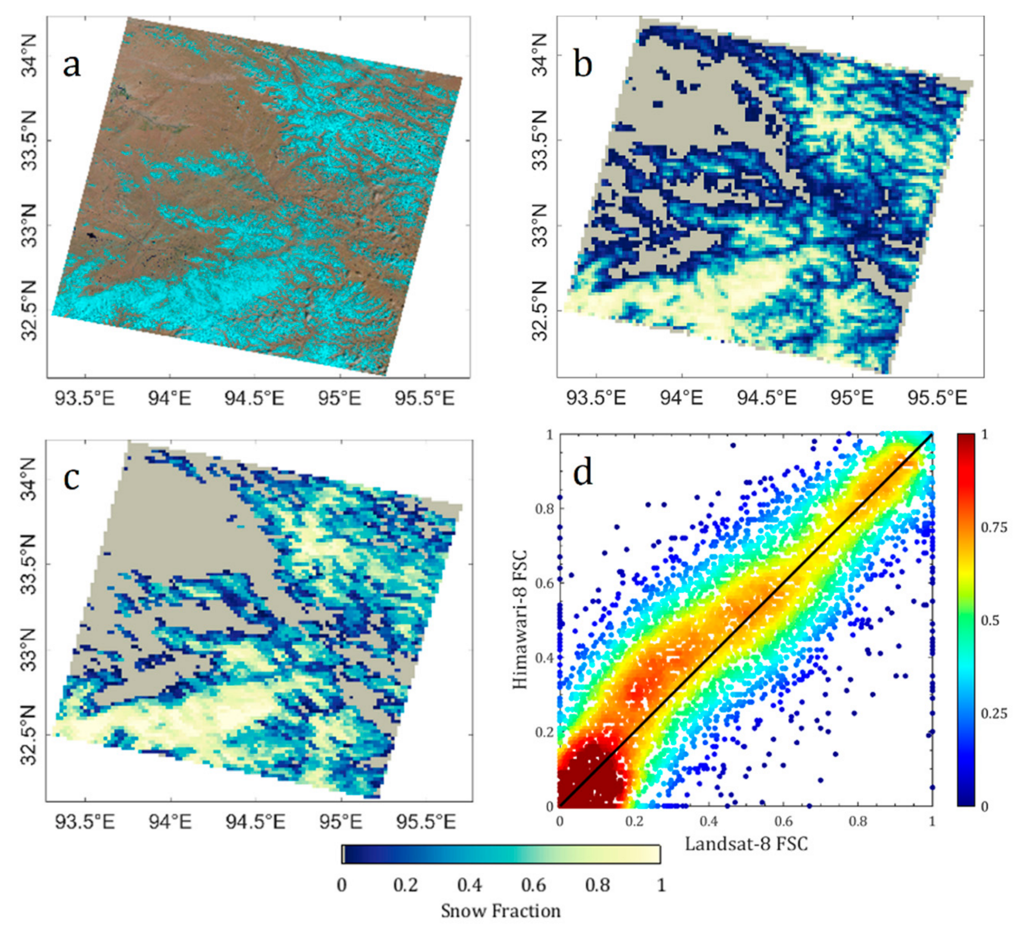
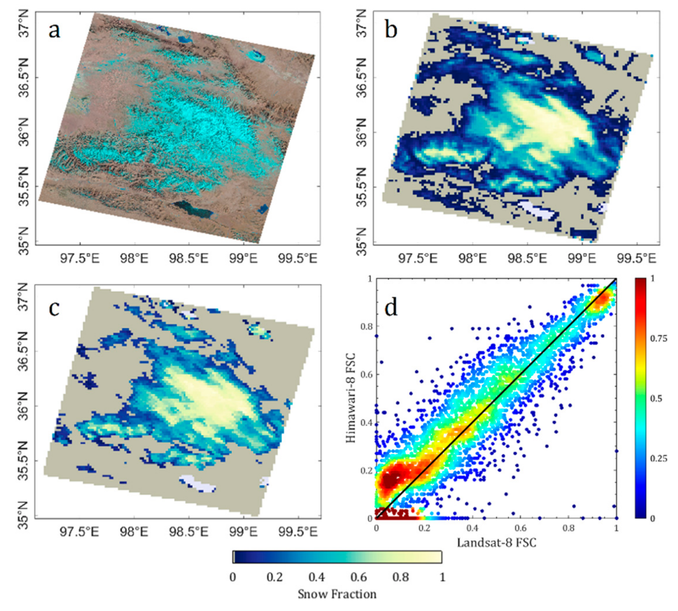
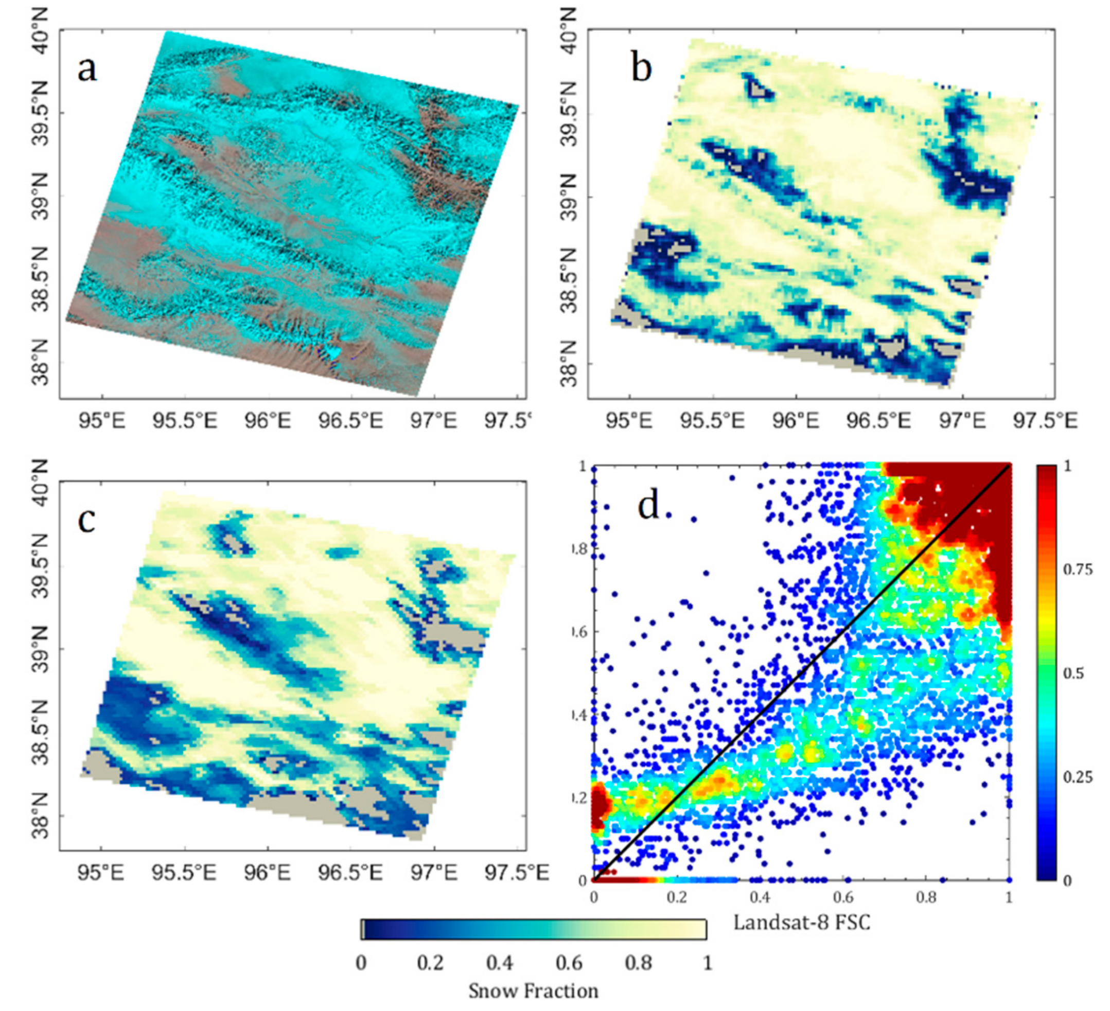
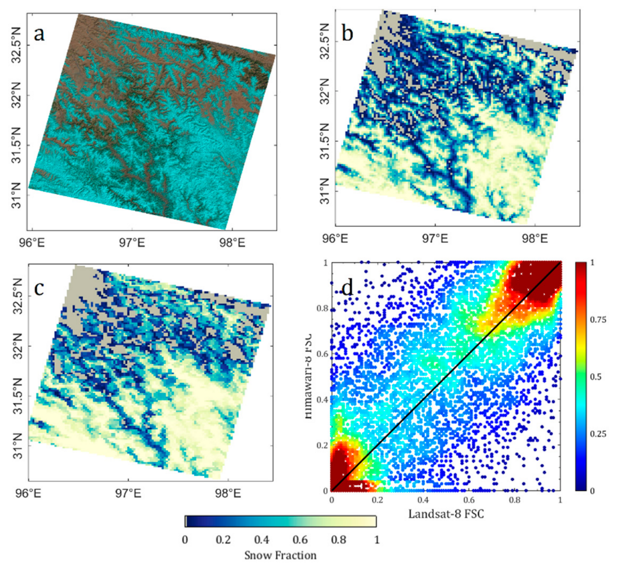
4.1. Evaluation Using Landsat–8 OLI

The instantaneous snow-covered area results between the Landsat–8 OLI (the location of OLI scenes is shown in Figure 1) and the Himawari–8 AHI over the Tibetan Plateau were compared. Due to the 10-min temporal resolution of Himawari–8 AHI observations, the difference of imaging time between the selected Himawari–8 AHI data and Landsat–8 OLI is not more than 5 min. We did so to reduce the uncertainties originating from the quick snowmelt and the discrepancy of illuminating conditions. The Himawari–8 AHI fractional snow cover image was cropped to match the small spatial extent of the Landsat–8 OLI fractional snow cover for comparison. The Landsat–8 OLI fractional snow cover at the spatial resolution of 30 m in the Universal Transverse Mercator (UTM) projection was then re-projected and resampled into the geographic projection with a grid size of 0.02° to match the Himawari–8 AHI fractional snow cover data. The resampling technique used here was to calculate the average fractional snow cover value of the corresponding small grid cells within the large grid cell.

For each Landsat–8 OLI scene, the evaluation metrics were calculated with the pixel-by-pixel fractional snow cover data pairs at a grid size of 0.02°. The comparison at the grid size of 0.04° was also performed because the pixel size of the Himawari–8 AHI imagery is stretched by 1.5–3 times over the Tibetan Plateau due to off-nadir viewing. The residual geolocation errors can be mitigated with the upscaling technique as well.

In

Table 3. Evaluation results of Himawari–8 instantaneous snow-covered area using Landsat–8 OLI data.

Land Cover	OLI Path/Row	Acquisition Day	Grid Size	Precision (Binary Metric)	Recall (Binary Metric)	OA (Binary Metric)	RMSE	R2
Forest	132/038	2016/02/29	0.02° 0.04°	0.78 0.80	0.98 0.99	0.83 0.85	0.18 0.15	0.81 0.88
	134/038	2016/02/27	0.02° 0.04°	0.88 0.91	0.96 0.96	0.87 0.90	0.19 0.14	0.75 0.83
Grassland	136/037	2016/10/22	0.02° 0.04°	0.89 0.90	0.93 0.95	0.89 0.93	0.15 0.09	0.81 0.91
	134/035	2016/01/26	0.02° 0.04°	0.86 0.89	0.92 0.92	0.92 0.93	0.08 0.07	0.90 0.96
	137/036	2017/11/01	0.02° 0.04°	0.88 0.91	0.95 0.96	0.89 0.92	0.14 0.10	0.86 0.92
	139/036	2017/11/15	0.02° 0.04°	0.82 0.85	0.90 0.92	0.90 0.92	0.16 0.11	0.84 0.90
Barren land	136/033	2016/01/08	0.02° 0.04°	0.95 0.96	0.97 0.97	0.92 0.92	0.20 0.16	0.74 0.81
	144/036	2016/10/14	0.02° 0.04°	0.85 0.87	0.92 0.94	0.89 0.90	0.18 0.13	0.83 0.89
	142/035	2017/10/19	0.02° 0.04°	0.85 0.86	0.89 0.91	0.92 0.93	0.13 0.09	0.86 0.92
Barren land (Himalaya)	138/040	2017/03/13	0.02° 0.04°	0.82 0.82	0.97 0.98	0.90 0.90	0.11 0.09	0.90 0.93
	137/040	2017/03/22	0.02° 0.04°	0.80 0.85	0.94 0.96	0.86 0.90	0.16 0.12	0.81 0.87
	142/040	2017/03/25	0.02° 0.04°	0.85 0.89	0.94 0.96	0.90 0.93	0.19 0.13	0.82 0.90

, we present the basic description of the evaluation results of the Himawari–8 AHI instantaneous snow-covered area. We selected the Landsat–8 OLI scenes that cover a spatial transition from snow-free ground to pure snow cover in mountainous areas to prevent fractional snow cover concentrating on low or high values, which would make the fractional snow cover comparison unrepresentative. The Landsat–8 OLI scenes used in this study encompassed three common land cover types (forest, grassland, and barren land) in the Tibetan Plateau. Additionally, Himalaya was included in the evaluation region. Hence, the effects of land cover type on Himawari–8 AHI fractional snow cover retrieval were inspected. The RMSE of the Himawari–8 AHI fractional snow cover was ≤ 0.20 at 0.02° resolution and ≤ 0.16 at 0.04° resolution for all the land cover types, which indicates that this algorithm outperformed MOD10A1, for which the RMSE is about 0.23 [23]. As the upscaling (aggregating) process generally reduces random errors, further upscaling to the tens-of-kilometers level resulted in error level lower than 0.1, which can satisfy the requirement of continental-scale application [71].

For Figure 7, Figure 8, Figure 9 and Figure 10, we chose four examples in the evaluation results to represent the Himawari–8 AHI fractional snow cover performance for grassland (Landsat–8 scene 136/037), sparse vegetation (Landsat–8 scene 134/035), barren land with very rugged terrain (Landsat–8 scene 136/033) and forest (Landsat–8 scene 134/038). The land surface of Landsat–8 scenes 136/037, 134/035, 136/033 and 134/038 has a relative altitude of 1600 m, 2500 m, 3300 m and 2100 m respectively.

Figure 7 shows the fractional snow cover results for the Landsat–8 OLI and the Himawari–8 AHI observations for a region with few trees. The south half of this Landsat–8 OLI scene covers the eastern part of the Tanggula Mountain. About 80% of this scene area is covered by grass in summer and there are headwaters of the Yangtze River and the Lancang River. There are some low clouds in this Landsat–8 OLI scene, which were identified in the QA image, and we excluded them from the snow cover mapping.

Figure 7b, c shows that patchy snow cover dominates this scene and that the Himawari–8 AHI fractional snow cover agrees well with the Landsat–8 OLI fractional snow cover with respect to the spatial distribution. The scatter plot in Figure 7d indicates that the relationship between the Himawari–8 AHI fractional snow cover and the Landsat–8 OLI fractional snow cover is approximately proportional. The overall accuracy of the Himawari–8 AHI fractional snow cover for this scene was up to 0.89, though Himawari-8 AHI omitted some fragmentary snow. As expected, the Himawari–8 AHI fractional snow cover performed better at the grid size of 0.04° than at the grid size of 0.02°. The RMSE of the Himawari–8 AHI fractional snow cover decreased from 0.15 to 0.09 and the R² increased from 0.81 to 0.91.

Figure 8 shows a case evaluation of the Himawari–8 AHI fractional snow cover with the Landsat–8 OLI data at a rugged region with sparse vegetation. This Landsat–8 OLI scene is located at the southwest of the Qinghai Lake and covers the eastern part of the Qaidam Basin. Water bodies were screened out during the generation of fractional snow cover maps. In this scene, though the Himawari–8 AHI fractional snow cover result omitted some snow-covered areas around the snowline, the comparison with the Landsat–8 OLI fractional snow cover showed surprisingly good correspondence, with an RMSE of 0.08 and an overall accuracy of 0.92. With a correlation coefficient of 0.96, the data points were highly concentrated around the 1:1 line in Figure 8d. This indicates that, sometimes, the Himawari–8 AHI fractional snow cover can be very accurate at the rugged areas, though the spatial resolution is relatively coarse.

A case study of the comparison between the Himawari–8 AHI fractional snow cover and the Landsat–8 OLI data for a barren and rugged area is shown in Figure 9. In this scene, much snow cover spreads over the south slopes and little can be found on the north slopes. The patchy snow cover on the north slopes detected by the Landsat–8 OLI tends to be omitted by the Himawari–8 AHI, probably due to the mixture with snow-free lands and shades at the relatively coarse resolution of the Himawari–8 AHI data.

The Himawari–8 AHI snow-covered area of this scene had a good overall accuracy of 0.92. However, unlike the good performance shown in Figure 8, the Himawari–8 AHI fractional snow cover of this scene resulted in an RMSE value of 0.20 and an R² value of 0.74. Even at the grid size of 0.04°, the RMSE of the Himawari–8 AHI fractional snow cover of this scene was greater than 0.10. In addition, the points did not gather around the 1:1 line. This indicates the complex terrain’s impact on the fractional snow cover retrieval based on this dynamic snow index method. The MOD10 snow-covered area has also been reported omission errors in mountainous areas [72]. Terrain shadows weaken snow’s reflected radiance, so in an image at a coarser resolution, snow is more difficult to detect. The absence of topographic correction limited the NDSI’s ability to represent snow’s spectral signal at the very rugged regions.

We also compared the instantaneous fractional snow cover between the Landsat–8 OLI and the Himawari–8 AHI to demonstrate the performance of Himawari–8 AHI snow-covered area retrieval in a forested area. Theoretically, the snow cover detected by multispectral imagers in space is the “exposed” snow cover. In other words, the snow cover under canopies of standing trees is obstructed at visible and infrared wavelengths.

In Figure 10, the comparison of the Himawari–8 AHI fractional snow cover and the Landsat–8 OLI fractional snow cover is shown. This Landsat–8 OLI scene is located at the eastern part of the Tibetan Plateau. Basically, the Himawari–8 AHI snow-covered area appeared similar with the Landsat–8 OLI in this scene. The points were not very close to the 1:1 line; the errors coincided well with the normal distribution. This inaccuracy may be partly associated with the relatively weak sensitivity of NDFSI to fractional snow cover over forested areas, and noise in the observation may be propagated into the fractional snow cover retrieval. Though NDFSI outperforms NDSI at detecting snow in evergreen coniferous forests, accurate snow cover mapping in forests is still difficult because a forest is a complex landscape that may consist of canopy, canopy-intercepted snow, snow-free ground, and snow-covered ground within gaps and tree shadows.

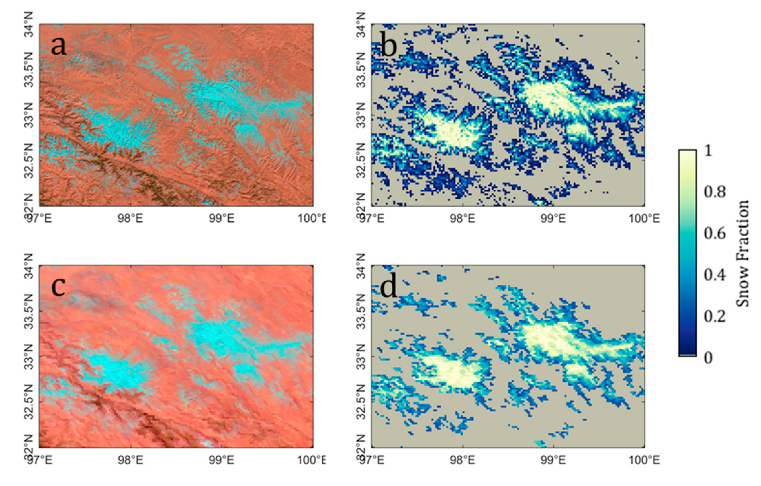
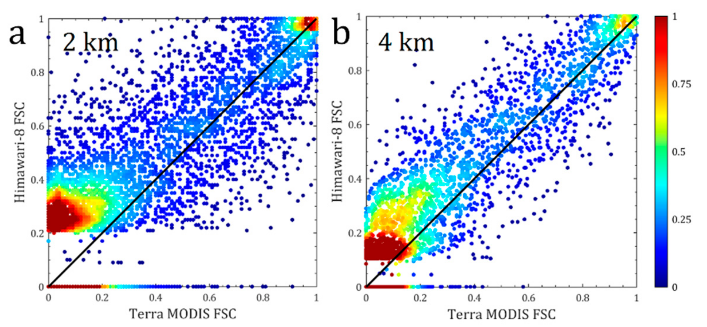
4.2. Evaluation Using Terra Moderate Resolution Imaging Spectrometer (MODIS)

Himawari–8 AHI fractional snow cover was also compared with MOD10A1 fractional snow cover estimated from Terra MODIS NDSI data (see the image’s spatial extent in Figure 1). Figure 11 illustrates an example of a fractional snow cover comparison, which was conducted for an eastern part of the Tibetan Plateau on 10 December 2016. Green grass dominates this region before snowfall, whereas forests are located mainly in the valleys of the Yangtze River, which is also known as the Jinsha River. As shown in Figure 11, the spatial distribution of Himawari–8 AHI fractional snow cover was quite consistent with MOD10A1 fractional snow cover, except for some patchy snow with low fractional snow cover.

The difference between Himawari–8 AHI fractional snow cover and MOD10A1 fractional snow cover is shown in the scatter plot of Figure 12. The pixel-by-pixel comparison indicates that Himawari–8 AHI overestimated snow of a fraction < 20% determined by MOD10A1. This is because MOD10A1 labeled as snow-free pixels of NDSI < 0, but the dynamic snow index method would result in fractional snow cover of > 0 for those pixels with a snow index value lower than 0 but higher than the snow-free background. A small number of points can be found for fractional snow cover of < 0.2 estimated by Himawari–8 AHI because the pixels of fractional snow cover < 0.2 with the 1.6 μm band reflectance > 0.2 were reassigned as snow-free to avoid spurious snow-covered area.

We also compared Himawari–8 AHI fractional snow cover and MOD10A1 fractional snow cover at the 4 km spatial scale to eliminate geolocation errors and the enlarged pixel effect from Himawari–8 AHI data. Taking MOD10A1 fractional snow cover as a reference, the RMSE value of Himawari–8 AHI fractional snow cover was about 0.19 at the 0.02° (about 2 km) scale and 0.10 at the 0.04° level. Moreover, the R² increased from 0.79 to 0.91 in the upscaling process. At the 0.04° level, Himawari–8 AHI fractional snow cover still slightly overestimated MOD10A1, probably due to the variant background information taken into consideration in the Himawari–8 AHI fractional snow cover retrieval.

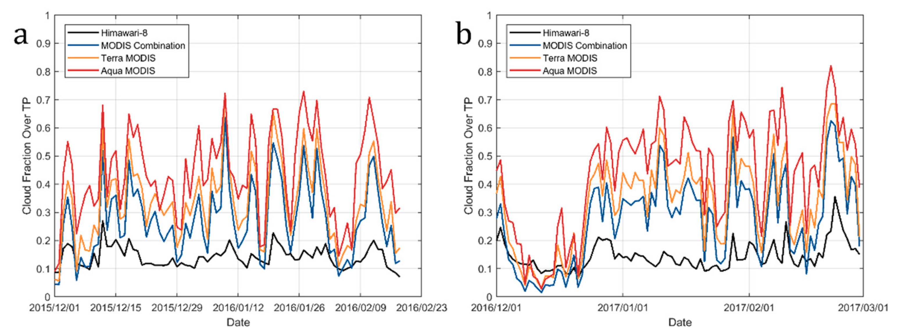
4.3. Cloud Removal Efficiency of Daily Composite Snow-Covred Area

With the aim of a spatially complete snow-covered area, the Himawari–8 AHI daily snow-covered area is the composite of all instantaneous daytime snow-covered area data available within a single day. The Cloud Mask Confidence Level Flag within the bit-packed QA layer of the Himawari–8 Level 2 Cloud Property product at 4 km was employed in this study to represent the cloud detection of Himawari–8 AHI imagery. The cloud removal efficiency of this temporal composite technique is subject to cloud persistence, observation intervals, and the cloud mask accuracy of the Himawari–8 Level 2 Cloud Property product. To demonstrate the cloud removal efficiency of Himawari–8 AHI observing the Earth at 10 min interval, its cloud coverage of the Tibetan Plateau was calculated and compared with that from MOD10C1 and MYD10C1. Figure 13 presents the daily cloud coverage of the Tibetan Plateau, of which the average was 34% and 33% in two winters (2015/2016 and 2016/2017), respectively, for the observation of Terra MODIS (MOD10C1), 44% and 43% for Aqua MODIS (MYD10C1), 27% for their combination, and 14% for the Himawari–8 AHI. The 2016/2017 winter had slightly less cloud coverage than 2015/2016 because the Tibetan Plateau was dominated by clear weather in December 2016.

Terra and Aqua MODIS instruments detect cloud coverage roughly in the range of 15%–45%. Aqua MODIS often detects more clouds than Terra MODIS and it may be partially due to their difference in satellite overpass time. Surprisingly, the Himawari–8 AHI Cloud Property product had more clouds than MODIS in December 2016, which is likely because the Himawari–8 cloud detection algorithm is “aggressive” at identifying clouds. A Himawari–8 AHI daily fractional snow cover image is shown in Figure 14. From Figure 14, it can be found that there are spatially extensive pixels labeled as cloudy in northern Tibet Plateau, which are in fact snow covered and under the clear-sky condition according to visual inspection. We look forward to improving the snow/cloud discrimination to avoid the cloud removal ability of Himawari–8 AHI being disturbed.

5. Discussion

Snow-covered area is an essential factor in surface energy balance and hydrological processes [56,73]. The National Research Council suggested that snow-covered area should have an accuracy of 10% or less at the spatial resolution of 50 km for continental-scale observations and 500 m for alpine-scale observations [71]. The World Meteorological Organization reported that snow-covered area requires a maximum uncertainty level of 10% for applications in agricultural meteorology and 20% for applications in the cryosphere (http://www.wmo-sat.info/oscar/requirements). However, many uncertainties have resulted in the RMSE of the Himawari–8 AHI snow-covered area algorithm being up to 0.20.

One main source of uncertainties is the sun–target–sensor geometry of Himawari–8 AHI imagery. Himawari–8 is located 35,793 km above the equator at 140.7°E, resulting in the viewing zenith angle over the Tibetan Plateau roughly ranging from 55° to 80°. As is shown in Figure 15, the pixel size in the north–south direction can be stretched by 1.5–3 times in most parts of the Tibetan Plateau region. Additionally, the pixel size in the west–east direction can be enlarged to 3–6 km as well, given that the spatial resolution of AHI’s bands 5 though 16 at nadir is 2 km. Signals of patchy and shallow snow are not likely to contribute much in such pixels; hence, the detection of snow cover may fail. Off-nadir viewing geometry not only enlarges the pixel but also elongates the atmospheric path. The absence of atmospheric correction of TOA reflectance in this study may have caused some inaccuracies for snow-covered area retrieval at the edges of the Himawari–8 AHI scanning range. Future studies will explore the effects of atmospheric correction using 6S [74], as well as the Himawari–8 aerosol optical thickness product and its cooperation with angular correction of reflectance.

Errors in the cloud-screening process have impacts on the retrieval of fractional snow cover as well. The erroneous identification of clear-sky conditions may lead to ice clouds being mistaken for snow. In addition, errors originating from cloud detection can propagate into the calculation of the snow index before snowfall. The NDSI/NDFSI value of clouds (water clouds in particular) may be mistaken for that of snow-free land. Consequently, fractional snow cover would be less accurate due to the errors from the cloud-screening process. However, the cloud detection issue in remote sensing technology has not been completely addressed yet. Clouds are found very often over the Tibetan Plateau in winter and the confusion between cloudy weather and clear skies is difficult to completely avoid when solely using spectral information. The terrain shadows within the Himawari–8 AHI imagery may result in uncertainties as well. At the edges of water bodies, the fractional snow cover may have been questionable in this study because we screened out water bodies before the retrieval process.

Unlike the MESMA for the fractional snow cover retrieval, the NDSI method is less physically reasonable but simpler and more feasible. The linear relationship between NDSI/NDFSI and fractional snow cover accounts for the varying land cover types and sun–target–sensor geometries, which is a step forward toward the MOD10 fractional snow cover algorithm. The varying snow properties (grain size and surface impurity) are not taken into consideration in the Himawari–8 AHI fractional snow cover estimation method. Therefore, the representation of fixed NDSI and NDFSI values for pure snow may be inappropriate. NDFSI is not as sensitive as NDSI to fractional snow cover, so the accuracy of fractional snow cover estimation in forests may be limited by the noise in NDFSI values.

An error analysis similar to the MOD10’s fractional snow cover retrieval method [17] was performed to investigate the variability in NDSI/NDFSI and the subsequent fractional snow cover estimation. The errors of fractional snow cover were associated with the variability of snow grain size, sun–target–sensor geometry, and atmospheric effect. It was assumed that each factor’s range is an approximation of ± 3σ and is normally distributed. The standard deviation, σ, was calculated for each factor and the root mean square of these factors gave a total error level. By using 50 and 1000 μm effective grain sizes for spherical particles with a solar zenith angle of 60°, snow directional-hemispherical reflectance was calculated based on the Mie scattering theory and the two-stream approximation to radiative transfer as aforementioned in Section 3.2. The Himawari–8 AHI cloud-free and snow-free reflectance data in November 2016 was also used. Then, we obtained a standard deviation of 0.0518 for the fractional snow cover. The effect of solar zenith angle was examined in a similar way. The solar zenith angle, with a range of 0°–80°, was used and the fractional snow cover result was a standard deviation of 0.0753. As we analyzed the effect of the viewing zenith angle varying from 0° to 80° in Section 3.2, a range of [0.67, 0.96] for NDSI and of [0.62, 0.96] for NDFSI can be assumed. That assumption would result in the fractional snow cover having a standard deviation of 0.112. The range of Himawari–8 AHI viewing zenith angle over the Tibetan Plateau is from 55° to 80°, hence a lower fractional snow cover variation can be expected. We also investigated atmospheric effect in the same way that Salomonson and Appel [17] did and the result was a standard deviation for fractional snow cover of 0.0226. Then, the square root of the sum-of-squares value for these factors was 0.146, which was close to the RMSE values listed in Table 3.

Though this dynamic snow index method is relatively simple and may have some uncertainties regarding variable imaging conditions and complex surface conditions, it is reasonable to monitor snow-covered areas with this method because the processing of massive amounts of geostationary weather satellite imagery can be complicated and time consuming.

6. Conclusions

Himawari–8 is a new geostationary weather satellite frequently observing East Asia and the Western Pacific Ocean. To explore the potential of snow cover monitoring over the Tibetan Plateau with this geostationary weather satellite, we developed a feasible methodology to estimate the snow-covered area (in the form of fractional snow cover) from the Himawari–8 AHI multispectral imagery. With the clouds screened out from instantaneous images acquired at daytime, the instantaneous fractional snow cover of each pixel is represented by the patchy snow and snow-free difference in snow indices divided by the difference of pure snow and snow-free ground. Considering the solar zenith angle, the daily composite of fractional snow cover images can be represented by reliable and cloud-free observations. This method does not require many computational resources and performs well over the Tibetan Plateau.

Compared with the Landsat–8 OLI snow-covered area generated with the MESMA method, the Himawari–8 AHI snow cover had an overall accuracy ranging from 0.83 to 0.93 over the Tibetan Plateau. As for the evaluation of fractional snow cover on the grid size of 0.02°, the Himawari–8 AHI fractional snow cover had RMSE values of 0.08–0.20 and R² values of 0.74–0.90. This method performed better for grasslands and sparsely vegetated lands and had errors higher than 0.15 over barren and rugged areas and forests. Considering the pixel size of the Himawari–8 AHI imagery at off-nadir conditions, this snow mapping method performed well based on the comparison with a grid size of 0.04°. Results of the 0.04° scale level revealed that the RMSE range was 0.07–0.16, the overall accuracy was 0.85–0.93, and the R² was 0.81–0.96. The daily composite of Himawari–8 AHI images generally reduces the cloud coverage in the Tibetan Plateau to 14%. It is an advantage over the combination of Terra and Aqua MODIS, which is about 27%. Notably, the Tibetan Plateau is close to the edge of Himawari–8’s full-disk image, and considering this, we look forward to extending this method to the high temporal observations of FY–4A (located at 104.7°E) for snow cover mapping.

For cloud-mitigated snow-covered area retrieval, the frequent multispectral images from geostationary weather satellites can be very helpful. Given that the geostationary weather satellite imagery of a spatially extensive area is acquired at various times of day, further efforts in snow-covered area mapping studies should consider improving the identification of clouds, shadows, and water bodies prior to fractional snow cover retrieval and making fractional snow cover retrieval more accurate by eliminating atmospheric and topographic effects.

References

1. Barnett, T.P.; Adam, J.C.; Lettenmaier, D.P. Potential impacts of a warming climate on water availability in snow-dominated regions. Nature 2005, 438, 303–309. [Google Scholar]
2. Winiger, M.; Gumpert, M.; Yamout, H. Karakorum–Hindukush–western Himalaya: Assessing high-altitude water resources. Hydrol. Process. 2005, 19, 2329–2338. [Google Scholar]
3. Su, F.; Zhang, L.; Ou, T.; Chen, D.; Yao, T.; Tong, K.; Qi, Y. Hydrological response to future climate changes for the major upstream river basins in the Tibetan Plateau. Glob. Planet. Chang. 2016, 136, 82–95. [Google Scholar]
4. Zhang, L.; Su, F.; Yang, D.; Hao, Z.; Tong, K. Discharge regime and simulation for the upstream of major rivers over Tibetan Plateau. J. Geophys. Res. Atmos. 2013, 118, 8500–8518. [Google Scholar]
5. Bookhagen, B.; Burbank, D.W. Toward a complete Himalayan hydrological budget: Spatiotemporal distribution of snowmelt and rainfall and their impact on river discharge. J. Geophys. Res. Earth Surf. 2010, 115, F03019. [Google Scholar]
6. Madan, N.J. Snow ecology: An interdisciplinary examination of snow-covered ecosystems. J. Ecol. 2001, 89, 1097–1098. [Google Scholar]
7. Zaitchik, B.F.; Rodell, M. Forward-looking assimilation of MODIS-derived snow-covered area into a land surface model. J. Hydrometeorol. 2009, 10, 130–148. [Google Scholar]
8. Hock, R.; Holmgren, B. A distributed surface energy-balance model for complex topography and its application to Storglaciären, Sweden. J. Glaciol. 2005, 51, 25–36. [Google Scholar]
9. Wu, T.; Qian, Z. The relation between the Tibetan winter snow and the Asian summer monsoon and rainfall: An observational investigation. J. Clim. 2003, 16, 2038–2051. [Google Scholar]
10. Xiao, Z.; Duan, A. Impacts of Tibetan Plateau snow cover on the interannual variability of the East Asian summer monsoon. J. Clim. 2016, 29, 8495–8514. [Google Scholar]
11. Zhang, Y.; Li, T.; Wang, B. Decadal change of the spring snow depth over the Tibetan Plateau: The associated circulation and influence on the East Asian summer monsoon. J. Clim. 2004, 17, 2780–2793. [Google Scholar]
12. Qian, Y.F.; Zheng, Y.Q.; Zhang, Y.; Miao, M.Q. Responses of China’s summer monsoon climate to snow anomaly over the Tibetan Plateau. Int. J. Climatol. 2003, 23, 593–613. [Google Scholar]
13. Li, W.; Guo, W.; Qiu, B.; Xue, Y.; Hsu, P.C.; Wei, J. Influence of Tibetan Plateau snow cover on East Asian atmospheric circulation at medium-range time scales. Nat. Commun. 2018, 9, 4243. [Google Scholar] [Green Version]
14. Dozier, J. Spectral signature of alpine snow cover from the Landsat Thematic Mapper. Remote Sens. Environ. 1989, 28, 9–22. [Google Scholar]
15. Kaufman, Y.J.; Kleidman, R.G.; Hall, D.K.; Martins, J.V.; Barton, J.S. Remote sensing of subpixel snow cover using 0.66 and 2.1 μm channels. Geophys. Res. Lett. 2002, 29, 1781. [Google Scholar]
16. Harrison, A.R.; Lucas, R.M. Multi-spectral classification of snow using NOAA AVHRR imagery. Int. J. Remote. Sens. 1989, 10, 907–916. [Google Scholar]
17. Salomonson, V.V.; Appel, I. Estimating fractional snow cover from MODIS using the normalized difference snow index. Remote Sens. Environ. 2004, 89, 351–360. [Google Scholar]
18. Painter, T.H.; Rittger, K.; McKenzie, C.; Slaughter, P.; Davis, R.E.; Dozier, J. Retrieval of subpixel snow covered area, grain size, and albedo from MODIS. Remote Sens. Environ. 2009, 113, 868–879. [Google Scholar] [Green Version]
19. Sirguey, P.; Mathieu, R.; Arnaud, Y. Subpixel monitoring of the seasonal snow cover with MODIS at 250 m spatial resolution in the Southern Alps of New Zealand: Methodology and accuracy assessment. Remote Sens. Environ. 2009, 113, 160–181. [Google Scholar]
20. Hall, D.K.; Riggs, G.A. Accuracy assessment of the MODIS snow products. Hydrol. Process. 2007, 21, 1534–1547. [Google Scholar]
21. Wang, X.; Xie, H.; Liang, T. Evaluation of MODIS snow cover and cloud mask and its application in Northern Xinjiang, China. Remote Sens. Environ. 2008, 112, 1497–1513. [Google Scholar]
22. Marchane, A.; Jarlan, L.; Hanich, L.; Boudhar, A.; Gascoin, S.; Tavernier, A.; Filali, N.; le Page, M.; Hagolle, O.; Berjamy, B. Assessment of daily MODIS snow cover products to monitor snow cover dynamics over the Moroccan Atlas mountain range. Remote Sens. Environ. 2015, 160, 72–86. [Google Scholar]
23. Rittger, K.; Painter, T.H.; Dozier, J. Assessment of methods for mapping snow cover from MODIS. Adv. Water Resour. 2013, 51, 367–380. [Google Scholar]
24. Hall, D.K.; Riggs, G.A.; Foster, J.L.; Kumar, S.V. Development and evaluation of a cloud-gap-filled MODIS daily snow-cover product. Remote Sens. Environ. 2010, 114, 496–503. [Google Scholar] [Green Version]
25. Morriss, B.F.; Ochs, E.; Deeb, E.J.; Newman, S.D.; Daly, S.F.; Gagnon, J.J. Persistence-based temporal filtering for MODIS snow products. Remote Sens. Environ. 2016, 175, 130–137. [Google Scholar] [Green Version]
26. Li, X.; Fu, W.; Shen, H.; Huang, C.; Zhang, L. Monitoring snow cover variability (2000–2014) in the Hengduan Mountains based on cloud-removed MODIS products with an adaptive spatio-temporal weighted method. J. Hydrol. 2017, 551, 314–327. [Google Scholar]
27. Dariane, A.B.; Khoramian, A.; Santi, E. Investigating spatiotemporal snow cover variability via cloud-free MODIS snow cover product in Central Alborz Region. Remote Sens. Environ. 2017, 202, 152–165. [Google Scholar]
28. Huang, Y.; Liu, H.; Yu, B.; Wu, J.; Kang, E.L.; Xu, M.; Wang, S.; Klein, A.; Chen, Y. Improving MODIS snow products with a HMRF-based spatio-temporal modeling technique in the Upper Rio Grande Basin. Remote Sens. Environ. 2018, 204, 568–582. [Google Scholar]
29. Dong, C.; Menzel, L. Producing cloud-free MODIS snow cover products with conditional probability interpolation and meteorological data. Remote Sens. Environ. 2016, 186, 439–451. [Google Scholar]
30. Dong, C.; Menzel, L. Improving the accuracy of MODIS 8-day snow products with in situ temperature and precipitation data. J. Hydrol. 2016, 534, 466–477. [Google Scholar]
31. Deng, J.; Huang, X.; Feng, Q.; Ma, X.; Liang, T. Toward improved daily cloud-free fractional snow cover mapping with multi-source remote sensing data in China. Remote Sens. 2015, 7, 6986–7006. [Google Scholar]
32. Dozier, J.; Painter, T.H.; Rittger, K.; Frew, J.E. Time–space continuity of daily maps of fractional snow cover and albedo from MODIS. Adv. Water Resour. 2008, 31, 1515–1526. [Google Scholar]
33. Romanov, P.; Tarpley, D. Enhanced algorithm for estimating snow depth from geostationary satellites. Remote Sens. Environ. 2007, 108, 97–110. [Google Scholar]
34. Romanov, P.; Gutman, G.; Csiszar, I. Satellite-derived snow cover maps for North America: Accuracy assessment. Adv. Space Res. 2002, 30, 2455–2460. [Google Scholar]
35. Romanov, P.; Gutman, G.; Csiszar, I. Automated monitoring of snow cover over North America with multispectral satellite data. J. Appl. Meteorol. 2000, 39, 1866–1880. [Google Scholar]
36. De Ruyter de Wildt, M.; Seiz, G.; Gruen, A. Operational snow mapping using multitemporal Meteosat SEVIRI imagery. Remote Sens. Environ. 2007, 109, 29–41. [Google Scholar]
37. Siljamo, N.; Hyvärinen, O. New geostationary satellite-based snow-cover algorithm. J. Appl. Meteorol. Clim. 2011, 50, 1275–1290. [Google Scholar]
38. Yang, J.; Jiang, L.; Shi, J.; Wu, S.; Sun, R.; Yang, H. Monitoring snow cover using Chinese meteorological satellite data over China. Remote Sens. Environ. 2014, 143, 192–203. [Google Scholar]
39. Wang, G.; Jiang, L.; Wu, S.; Shi, J.; Hao, S.; Liu, X. Fractional snow cover mapping from FY-2 VISSR imagery of China. Remote Sens. 2017, 9, 983. [Google Scholar]
40. Bessho, K.; Date, K.; Hayashi, M.; Ikeda, A.; Imai, T.; Inoue, H.; Kumagai, Y.; Miyakawa, T.; Murata, H.; Ohno, T.; et al. An introduction to Himawari–8/9-Japan’s new-generation geostationary meteorological satellites. J. Meteorol. Soc. Jpn. 2016, 94, 151–183. [Google Scholar]
41. Qiu, J. China: The third pole. Nature 2008, 454, 393–396. [Google Scholar] [Green Version]
42. Zhang, Y.; Li, B.; Zheng, D. Datasets of the boundary and area of the Tibetan Plateau. Acta Geogr. Sin. 2002, 69, 164–168. [Google Scholar]
43. Gao, Q.; Guo, Y.; Xu, H.; Ganjurjav, H.; Li, Y.; Wan, Y.; Qin, X.; Ma, X.; Liu, S. Climate change and its impacts on vegetation distribution and net primary productivity of the alpine ecosystem in the Qinghai-Tibetan Plateau. Sci. Total. Environ. 2016, 554–555, 34–41. [Google Scholar]
44. Miller, D.J. Grasslands of the Tibetan plateau. Rangelands 1990, 12, 159–163. [Google Scholar]
45. Li, P.; Mi, D. Distribution of snow cover in China. J. Glaciol. Geocryol. 1983, 5, 9–18. [Google Scholar]
46. Qin, D.; Liu, S.; Li, P. Snow Cover Distribution, Variability, and Response to Climate Change in Western China. J. Clim. 2006, 19, 1820–1833. [Google Scholar]
47. Wang, J.; Che, T.; Li, Z.; Li, H.; Hao, X.; Zheng, Z.; Xiao, P.; Li, X.; Huang, X.; Zhong, X.; et al. Investigation on snow characteristics and their distribution in China. Adv. Earth. Sci. 2018, 33, 12–26. [Google Scholar]
48. Japan Meteorological Agency. Himawari–8/9 Himawari standard data user’s guide (version 1.3), Version 1.3 ed.; Japan Meteorological Agency: Tokyo, Japan, 2017. [Google Scholar]
49. Imai, T.; Yoshida, R. Algorithm theoretical basis for Himawari–8 cloud mask product. Meteorol. Satell. Center Tech. Note 2016, 61, 1–17. [Google Scholar]
50. Shi, J. An automatic algorithm on estimating sub-pixel snow cover from MODIS. Quat. Sci. 2012, 32, 6–15. [Google Scholar]
51. Hao, S.; Jiang, L.; Shi, J.; Wang, G.; Liu, X. Assessment of MODIS-based fractional snow cover products over the Tibetan Plateau. IEEE J. Sel. Top. Appl. Earth Obs. Remote Sens. 2018, 12, 533–548. [Google Scholar]
52. Barsi, J.A.; Lee, K.; Kvaran, G.; Markham, B.L.; Pedelty, J.A. The spectral response of the Landsat–8 operational land imager. Remote Sens. 2014, 6, 10232–10251. [Google Scholar]
53. Lee, S.; Klein, A.G.; Over, T.M. A comparison of MODIS and NOHRSC snow-cover products for simulating streamflow using the Snowmelt Runoff Model. Hydrol. Process. 2005, 19, 2951–2972. [Google Scholar]
54. Wulf, H.; Bookhagen, B.; Scherler, D. Differentiating between rain, snow, and glacier contributions to river discharge in the western Himalaya using remote-sensing data and distributed hydrological modeling. Adv. Water Resour. 2016, 88, 152–169. [Google Scholar] [Green Version]
55. He, Z.H.; Parajka, J.; Tian, F.Q.; Blöschl, G. Estimating degree-day factors from MODIS for snowmelt runoff modeling. Hydrol. Earth. Syst. Sc. 2014, 18, 4773–4789. [Google Scholar] [Green Version]
56. Liu, Y.; Peters-Lidard, C.D.; Kumar, S.; Foster, J.L.; Shaw, M.; Tian, Y.; Fall, G.M. Assimilating satellite-based snow depth and snow cover products for improving snow predictions in Alaska. Adv. Water Resour. 2013, 54, 208–227. [Google Scholar]
57. Ek, M.B.; Mitchell, K.E.; Lin, Y.; Rogers, E.; Grunmann, P.; Koren, V.; Gayno, G.; Tarpley, J.D. Implementation of Noah land surface model advances in the National Centers for Environmental Prediction operational mesoscale Eta model. J. Geophys. Res. 2003, 108, 8851. [Google Scholar]
58. Wang, X.; Xie, H. New methods for studying the spatiotemporal variation of snow cover based on combination products of MODIS Terra and Aqua. J. Hydrol. 2009, 371, 192–200. [Google Scholar]
59. Riggs, G.A.; Hall, D.K. MODIS snow products collection 6 user guide. Digit. Media 2015, 66, 1–66. [Google Scholar]
60. Salomonson, V.V.; Appel, I. Development of the Aqua MODIS NDSI fractional snow cover algorithm and validation results. IEEE. Trans. Geosci. Remote 2006, 44, 1747–1756. [Google Scholar]
61. Amante, C. ETOPO1 1 arc-minute global relief model: procedures, data sources and analysis; NOAA NESDIS: Boudler, CO, USA, 2009. [Google Scholar]
62. Chen, J.; Chen, J.; Liao, A.; Cao, X.; Chen, L.; Chen, X.; He, C.; Han, G.; Peng, S.; Lu, M.; et al. Global land cover mapping at 30m resolution: A POK-based operational approach. ISPRS J. Photogramm. 2015, 103, 7–27. [Google Scholar] [Green Version]
63. Salisbury, J.W. Johns Hopkins University spectral library and ASTER spectral library. 2002. Available online: http://speclib.jpl.nasa.gov (accessed on 28 June 2004).
64. Wang, X.; Wang, J.; Jiang, Z.; Li, H.; Hao, X. An effective method for snow-cover mapping of dense coniferous forests in the Upper Heihe River Basin using Landsat Operational Land Imager data. Remote Sens. 2015, 7, 17246–17257. [Google Scholar]
65. Riggs, G.A.; Hall, D.K.; Salomonson, V.V. MODIS snow products user guide to collection 5. Digit. Media 2006, 80, 1–80. [Google Scholar]
66. Tanikawa, T.; Aoki, T.; Hori, M.; Hachikubo, A.; Aniya, M. Snow bidirectional reflectance model using non-spherical snow particles and its validation with field measurements. EARSeL eProceedings 2006, 5, 137–145. [Google Scholar]
67. Aoki, T.; Aoki, T.; Fukabori, M.; Hachikubo, A.; Tachibana, Y.; Nishio, F. Effects of snow physical parameters on spectral albedo and bidirectional reflectance of snow surface. J. Geophys. Res. Atmos. 2000, 105, 10219–10236. [Google Scholar] [Green Version]
68. Kokhanovsky, A.A.; Breon, F.M. Validation of an analytical snow BRDF model using PARASOL multi-angular and multispectral observations. IEEE Geosci. Remote S 2012, 9, 928–932. [Google Scholar]
69. Leroux, C.; Deuzé, J.L.; Goloub, P.; Sergent, C.; Fily, M. Ground measurements of the polarized bidirectional reflectance of snow in the near-infrared spectral domain: Comparisons with model results. J. Geophys. Res. Atmos. 1998, 103, 19721–19731. [Google Scholar]
70. Roujean, J.-L.; Leroy, M.; Deschamps, P.-Y. A bidirectional reflectance model of the Earth’s surface for the correction of remote sensing data. J. Geophys. Res. Atmos. 1992, 97, 20455–20468. [Google Scholar]
71. National Research Council. Prospects and concerns for satellite remote sensing of snow and ice; National Academy Press: Washington, DC, USA, 1989.
72. Huang, X.; Liang, T.; Zhang, X.; Guo, Z. Validation of MODIS snow cover products using Landsat and ground measurements during the 2001–2005 snow seasons over northern Xinjiang, China. Int. J. Remote. Sens. 2011, 32, 133–152. [Google Scholar]
73. Tahir, A.A.; Chevallier, P.; Arnaud, Y.; Ashraf, M.; Bhatti, M.T. Snow cover trend and hydrological characteristics of the Astore River basin (Western Himalayas) and its comparison to the Hunza basin (Karakoram region). Sci. Total. Environ. 2015, 505, 748–761. [Google Scholar]
74. Vermote, E.F.; Tanré, D.; Deuze, J.L.; Herman, M.; Morcette, J.-J. Second simulation of the satellite signal in the solar spectrum, 6S: An overview. IEEE. Trans. Geosci. Remote 1997, 35, 675–686. [Google Scholar]
Figure 1. The land cover type map of the Tibetan Plateau. The spatial extent of Landsat–8 Operational Land Imager (OLI) and Moderate Resolution Imaging Spectroradiometer (MODIS) data used in this study is shown as well.
Remotesensing 11 02391 g001
Figure 2. The snow cover duration (SCD) of the Tibetan Plateau [47].
Remotesensing 11 02391 g002
Figure 3. Reflectance of snow, water cloud, vegetation, soil, and water.
Remotesensing 11 02391 g003
Figure 4. Fractional snow cover versus normalized difference snow index (NDSI) on soil background.
Remotesensing 11 02391 g004
Figure 5. Fractional snow cover versus normalized difference snow index (NDSI) (a) and normalized difference forest–snow index (NDFSI) (b) on vegetation background.
Remotesensing 11 02391 g005
Figure 6. Flowchart of Himawari–8 AHI fractional snow cover retrieval.
Remotesensing 11 02391 g006
Figure 7. A case evaluation of Himawari–8 AHI fractional snow cover with Landsat–8 data for grassland: (a) Landsat–8 OLI image at the Worldwide Reference System-2 (WRS-2) Path/Row of 136/037 on 22 October 2016; (b) the corresponding Landsat–8 OLI fractional snow cover; (c) the corresponding Himawari–8 AHI fractional snow cover at UTC 4:10 a.m.; (d) the scatter plot displaying 8765 points of Himawari–8 AHI fractional snow cover versus Landsat–8 fractional snow cover at a 0.02° resolution. The Landsat–8 OLI natural color images shown hereafter are the composite of surface reflectance data from bands 6, 5, and 4 after gamma correction with the parameter of 0.5.
Remotesensing 11 02391 g007
Figure 8. A case evaluation of Himawari–8 AHI fractional snow cover with Landsat–8 data for a rugged and sparsely vegetated area: (a) the Landsat–8 OLI image at WRS-2 134/035 on 26 January 2016; (b) the corresponding Landsat–8 fractional snow cover; (c) the corresponding Himawari–8 AHI fractional snow cover at UTC 4:00 a.m.; (d) the scatter plot displaying 8999 points of Himawari–8 AHI fractional snow cover versus Landsat–8 fractional snow cover at a 0.02° resolution.
Remotesensing 11 02391 g008
Figure 9. A case evaluation of Himawari–8 AHI fractional snow cover with Landsat–8 data for a very rugged area: (a) Landsat–8 OLI image at WRS-2 136/033 on 8 January 2016; (b) the corresponding Landsat–8 fractional snow cover; (c) the corresponding Himawari–8 AHI fractional snow cover at UTC 4:10 a.m.; (d) the scatter plot displaying 9435 points of Himawari–8 AHI fractional snow cover versus Landsat–8 fractional snow cover at a 0.02° resolution.
Remotesensing 11 02391 g009
Figure 10. A case evaluation of Himawari–8 AHI fractional snow cover with Landsat–8 data for vegetated land: (a) Landsat–8 OLI image at WRS 134/038 on 27 February 2016; (b) the corresponding Landsat–8 fractional snow cover; (c) the corresponding Himawari–8 AHI fractional snow cover at UTC 4:00 a.m.; (d) the scatter plot displaying 10,394 points of Himawari–8 AHI fractional snow cover versus Landsat–8 fractional snow cover at a 0.02° resolution.
Remotesensing 11 02391 g010
Figure 11. A case evaluation of Himawari–8 AHI fractional snow cover with MOD10A1: (a) the Terra MODIS image (bands 5, 4, and 3) of an eastern part of the Tibetan Plateau on 10 December 2016; (b) the corresponding MOD10A1 fractional snow cover; (c) the corresponding Himawari–8 AHI image at UTC 4:20 a.m.; (d) the Himawari–8 AHI fractional snow cover.
Remotesensing 11 02391 g011
Figure 12. The scatter plot of Himawari–8 AHI fractional snow cover with MOD10A1 at the spatial scale of 2 km with 15,000 points (a) and of 4 km with 3750 points (b).
Remotesensing 11 02391 g012
Figure 13. The Tibetan Plateau’s cloud coverage fraction from Himawari–8 AHI and MODIS in the winter season of 2015/2016 (a) and 2016/2017 (b).
Remotesensing 11 02391 g013
Figure 14. The Himawari–8 AHI daily fractional snow cover of the Tibetan Plateau on 17 January 2016.
Remotesensing 11 02391 g014
Figure 15. The rate of Himawari–8 AHI’s pixel size expansion in the north–south (a) and west–east (b) directions.
Remotesensing 11 02391 g015