Article

The Effect of Mineral Sediments on Satellite Chlorophyll-a Retrievals from Line-Height Algorithms Using Red and Near-Infrared Bands

Water Science and Technology Directorate, Environment and Climate Change Canada, 867 Lakeshore Rd, Burlington, ON L7S 1A1, Canada
*
Author to whom correspondence should be addressed.
Remote Sens. 2019, 11(19), 2306; https://doi.org/10.3390/rs11192306
Submission received: 12 August 2019 / Revised: 24 September 2019 / Accepted: 27 September 2019 / Published: 3 October 2019

Abstract

:
Red and near-infrared line-height algorithms such as the maximum chlorophyll index (MCI) are often considered optimal for remote sensing of chlorophyll-a (Chl-a) in turbid eutrophic waters, under the assumption of minimal influence from mineral sediments. This study investigated the impact of mineral turbidity on line-height algorithms using MCI as a primary example. Inherent optical properties from two turbid eutrophic lakes were used to simulate reflectance spectra. The simulated results: (1) confirmed a non-linear relationship between Chl-a and MCI; (2) suggested optimal use of the MCI at Chl-a < ~100 mg/m3 and saturation of the index at Chl-a ~300 mg/m3; (3) suggested significant variability in the MCI:Chl-a relationship due to mineral scattering, resulting in an RMSE in predicted Chl-a of ~23 mg/m3; and (4) revealed elevated Chl a retrievals and potential false positive algal bloom reports for sediment concentrations > 20 g/m3. A novel approach combining both MCI and its baseline slope, MCIslope reduced the RMSE to ~5 mg/m3. A quality flag based on MCIslope was proposed to mask erroneously high Chl-a retrievals and reduce the risk of false positive bloom reports in highly turbid waters. Observations suggest the approach may be valuable for all line-height-based Chl-a algorithms.

Graphical Abstract

1. Introduction

Remote sensing is increasingly being used as a complementary approach to conventional ground-based water quality monitoring of inland waters [1,2,3], with applications supporting water resource management, protecting ecosystem services, and furthering our understanding of lake biogeochemical processes [4]. Of particular concern in many coastal and inland waters is the occurrence of potentially harmful cyanobacteria blooms, which can pose serious threats to the integrity of fresh and marine aquatic ecosystems and significant public health risks [5,6,7,8]. Numerous algorithms have been developed for the estimation of chlorophyll-a (Chl-a) concentrations from aquatic colour remote sensing (see references [9,10] for reviews), allowing the production of synoptic mapped algal bloom conditions for water quality managers and other water resource stakeholders. Algorithms are often implemented using different spectral ranges for different water types. For example, the blue/green (B/G) reflectance ratio [10,11,12] is considered optimal for Case 1 or oligotrophic waters, whereas algorithms targeting spectral features in the red–near-infrared (R-NIR) are frequently applied to turbid eutrophic waters [2,13,14]. Two main strategies have been used for Chl-a algorithms using R-NIR wavebands: band-ratios and peak line-height measures. Band-ratio algorithms taking the form of two-band [15], three-band [13], and four-band [16] models have been applied to a range of turbid eutrophic waters. The R-NIR line-height algorithms measure the height of a reflectance peak or trough associated with an algal or cyanobacterial fluorescence, absorption or scattering feature relative to a baseline typically defined by two wavelengths either side of that spectral feature. Such line-height algorithms include the cyanobacteria index (CI; [17]), fluorescence line height (FLH; [18]), maximum chlorophyll index (MCI; [14]), and maximum peak height (MPH; [2]).
The R-NIR algorithms based on band ratios or line-heights are particularly favourable for studying eutrophication and algal/cyanobacterial blooms in optically complex coastal and inland waters. Coloured dissolved organic matter (CDOM) absorption decreases exponentially from blue to red wavelengths so, in many cases, with the exception perhaps of highly dystrophic systems, the contribution of CDOM to optical properties in the R-NIR may be considered negligible. Line-height algorithms are also considered to be less sensitive to the uncertainties in atmospheric correction [19], which can limit the usefulness of band ratios over highly turbid or eutrophic waters (particularly B/G where those uncertainties are often exacerbated). Indeed the application of line-height algorithms to uncorrected top-of-atmosphere (TOA) or partially atmospherically-corrected (using bottom of Rayleigh reflectance, BRR) image products has gained popularity in recent years [1,20,21,22]. Under the assumption that the effect of mineral suspended particulate matter (MSPM) on these line-height algorithms is also minimal, they are frequently applied in coastal and inland water environments prone to high riverine sediment loads, resuspension events, and nearshore erosion. For example, Gower et al. [23] suggested the MCI allowed the detection of blooms in sediment-laden plumes of the Fraser River in the eastern Strait of Georgia. Binding et al. [24] noted the absence of elevated MCI in known mineral turbidity zones in Lake Erie, while the CI of [17] is applied in NOAA’s operational harmful algal bloom (HAB) Bulletin to track blooms in the shallow, turbid western basin of Lake Erie [3]. The MCI is also used routinely by Environment and Climate Change Canada (ECCC) to monitor the progression of intensive blooms in the shallow, turbid waters of Lake Winnipeg [1].
Despite previous validation of these approaches and confidence in their suitability for monitoring intense blooms, instances were noted whereby under conditions of extreme sediment load false positive bloom reports were occurring. Motivation for this study was therefore driven by a need to understand the effect of suspended sediments on chlorophyll retrievals and reduce uncertainties associated with bloom reports under highly turbid conditions. There has been some effort to consider the impact of mineral suspended particulate matter (MSPM) on Chl-a retrieval algorithms, such as the three-band ratio with an NIR band [25], a four-band ratio [16], and others [26]. These studies, however, mitigate the effect of mineral turbidity by choosing band combinations from the best regression agreement with Chl-a, without investigating the mechanisms by which MSPM affects the algorithms, and quantitatively computing the impact of MSPM on Chl-a retrievals. Furthermore, due to the scarcity of in situ datasets, algorithms are often derived over small Chl-a ranges (e.g., ~0–20 μg/L in reference [27]), have a limited number of data points (e.g., eight samples in reference [28]), or show irregular distribution of Chl-a concentrations over the range [29]. Such confounding factors in the process of algorithm development and validation limit the reliability and transferability of proposed models. It would therefore be useful to understand Chl-a algorithm performances over a wide range of biogeochemical conditions consistent with the natural variability observed in the field. To address such concerns, radiative transfer models can be used to build simulated reflectance spectra to provide adequate data density over the range of conditions representative of coastal and inland waters. Such simulations can be carried out using radiative transfer programs such as Hydrolight/Ecolight [30,31].
In this study, we used both in situ and simulated datasets to investigate the impact of mineral turbidity on R-NIR line-height Chl-a algorithms, using the MCI as a primary example, and explore potential solutions to mitigate MSPM-related uncertainties in Chl-a retrievals from the MCI and other line-height algorithms. We addressed the problem by: (a) applying a large historical database of in situ optical properties measured in turbid, eutrophic lakes, to compare in situ reflectance with results of radiative transfer simulations; (b) generating reflectance spectra for a range of Chl-a and MSPM concentrations to analyze the impact of MSPM on the relationship between MCI and Chl-a; and (c) exploring novel solutions to minimize the effect of MSPM on MCI-derived Chl-a.

2. Methods

2.1. Study Areas

Observations from two large North American lakes were used in this study. Lake Winnipeg (LW) is a turbid eutrophic lake in Manitoba, Canada, which has experienced accelerated nutrient loading over the last two decades leading to a substantial increase in the frequency, severity, and extent of algal blooms [1,32,33]. Lake Erie (LE) is the most biologically productive of the Laurentian Great Lakes and has suffered a resurgence of harmful algal blooms in the last decade, particularly in the turbid west basin [3,7]. Both lakes are fairly shallow (LW average depth ~19 m, west basin of LE average ~7 m), with substantial influence from river loadings of mineral sediments, shoreline erosion, and resuspension events, providing an ideal dataset for studying the impact of mineral sediments on chlorophyll-retrieval algorithms.

2.2. In Situ Biogeochemistry and Optical Measurements

A Hyperspectral Profiler II (Satlantic Inc., Halifax, NS, USA, now Seabird Scientific) was deployed at each station to measure profiles of upwelling radiance (Lu) and downwelling plane irradiance (Ed) at 2–3 nm intervals from 350–800 nm. The remote sensing reflectance, Rrs (λ, 0+) was calculated as Lu/Ed after extrapolation to the surface and correction for interactions at the air-water interface following Mueller et al. (2003) [34]. Profiles exhibiting ship shadow effects, low light levels, poor extrapolation, or otherwise erroneous profiles were quality flagged and removed from the analysis. The ECO-triplet sensors (Wetlabs, Philomath OR) were deployed for in situ spectral particulate backscatter measurements at six custom wavelengths (532, 630, 650, 676, 700 and 880 nm).
Particulate absorption was measured using the quantitative filter technique with a VARIAN Cary-300 dual-beam spectrophotometer after filtering surface water samples onto 47 mm Whatman GF/C filters, scanning from 350 to 750 nm at 1 nm increments (see reference [35]). Filters were placed on a glass slide directly in front of the detector window and the optical density of the sample was measured relative to a reference filter treated with distilled water. A pathlength amplification factor was applied following the theoretical calculations of [36] and residual scattering correction (assuming negligible absorption in the NIR) was carried out by normalizing spectra to the average absorption measured between 740–750 nm assuming no wavelength dependence. Removal of pigmented material using sodium hypochlorite enabled the partition of a*Total, a*Ph, and a*NAP as the total, phytoplankton, and non-algal particulate (including both mineral and organic detrital material) absorption fractions, respectively. Here we assumed a*NAP was dominated by mineral absorption and, thus, denoted this as a*MSPM from this point on. Spectral absorption by CDOM was measured spectrophotometrically after filtration though 0.45 μm cellulose acetate filters, with distilled water at the same ambient temperature used as a reference. The ranges of measured aCDOM(440) (CDOM absorption at 440 nm) are shown in Table 1. The analysis of Chl-a was carried out by Environment and Climate Change Canada (ECCC)’s National Laboratory for Environmental Testing. Surface water was filtered through 47 mm GFC filters and frozen immediately. After extraction with 90% acetone, Chl-a concentrations were determined spectrophotometrically using the trichromatic equations in SCOR-UNESCO [37]. Suspended particulate matter (SPM) was measured gravimetrically after filtering surface water onto pre-rinsed and weighed 47 mm GFC filters. Filters were subsequently reweighed after drying overnight at 80 °C and again after ashing (3 h at 500 °C) to provide concentrations of total SPM and MSPM, respectively. Data from several inland water research and monitoring cruises between 2011 and 2015 on board the CCGS Limnos and MV Namao provided a wide range of biogeochemical and optical conditions on the two lakes (see Table 1). Table 1 presents the number of observations used in this study and the range of water constituent concentrations measured on both lakes, which were used both as input to Ecolight for model validation purposes and as a guide to determine the appropriate ranges over which reflectance was simulated.

2.3. Rrs Modelling

Hydrolight-Ecolight 5.2 [30,31] is a widely used radiative transfer program for bio-optical modelling, allowing the simulation of spectral Rrs by defining the concentrations and absorption, scattering, and fluorescence properties for both Case 1 waters and for non-covarying components of Case 2 waters. This study used Ecolight, a faster version of Hydrolight which solves the azimuthally averaged radiative transfer equation to simulate nadir viewing Rrs. A typical Case 2 model in Ecolight was employed, with four components: pure water (w), phytoplankton (Ph), CDOM, and MSPM. As input for the model, default water absorption and backscatter of pure water was chosen in Ecolight 5.2 [31,38]. User-defined absorption (a) and backscattering (bb) coefficients were used according to Equations (1)–(3).
a ( λ ) = a w ( λ ) + a * P h ( λ ) · [ Chl-a ] + a * M S P M ( λ ) · [ M S P M ] + a * C D O M ( λ ) · [ C D O M ]
b b ( λ ) = b b   w ( λ ) + b b * P h ( λ ) · [ Chl-a ] + b b * M S P M ( λ ) · [ M S P M ]
a * P h ( λ ) = A × [ Chl-a ] B
where a* and bb* represent the concentration-specific inherent optical properties (SIOPs), [MSPM], [Chl-a] are the concentrations of MSPM, and chlorophyll-a respectively and [CDOM] is CDOM absorption at 440 nm. Considering the pigment package effect of chlorophyll-a [39,40], a chlorophyll-a dependent a*Ph(λ) was adopted as defined in Equation (3), following Bricaud et al. [41]. Concentration-specific absorption (a*) for CDOM and MSPM were determined by linear regression on their contributions to total absorption (aCDOM and aMSPM, respectively), while the A and B coefficients for a*Ph (Equation (3)) were fitted simultaneously using a least-squares optimization of the relationship between [Chl-a] and a*Ph(λ) calculated as aPh(λ)/[Chl-a]. Multiple linear regression was used to obtain the average concentration-specific backscatter for phytoplankton (bb*Ph) and MSPM (bb*MSPM) for each of the spectral bb channels of the ECO-triplet sensors, and then linearly interpolated between those channels. With weak absorption of CDOM in the R-NIR, previous studies [24,42] have shown that aCDOM(440) < 1 m−1 has limited effect on Rrs simulation in this spectral range; therefore, aCDOM(440) was kept at a constant lake-average of 0.994 m−1 for all simulations.
Average weather and viewing conditions from in situ samples were employed in the Rrs simulation, including a constant solar zenith angle of 30°, average cloud cover of 39.5%, and an average wind speed of 4.85 m/s. The simulations consider inelastic scattering, including the chlorophyll-a fluorescence with a default fluorescence efficiency of 0.02. All simulations were set to be optically deep under the condition of negligible contribution to Rrs from the substrate, a reasonable assumption for R-NIR wavelengths in turbid waters. Vertical profiles of biogeochemical constituents and optical properties were not available at all sites; therefore, constant vertical profiles equal to surface measures were used under the assumption of a vertically mixed water column. Such an assumption may not hold where calm conditions may have allowed algal biomass to accumulate at the surface under bloom conditions. The remaining parameters were set to default within Ecolight, including a RADTRAN-X sky model.

2.4. MCI Calculation and Performance Assessment

Modelled and in situ measured spectral reflectance were used to calculate simulated and observed MCI, respectively. The MCI and other line-height algorithms are defined as the height of a peak (or trough) in spectral radiance or reflectance at a waveband centered at λ2, relative to a baseline extrapolated between bands either side of that spectral feature at λ1 and λ3 as shown in Equation (4) [14,17]:
M C I = R rs ( λ 2 ) R rs ( λ 1 ) λ 2 λ 1 λ 3 λ 1 · [ R rs ( λ 3 ) R rs ( λ 1 ) ]
For the ocean and land colour instrument (OLCI) sensor onboard ESA’s Sentinel-3 satellite, and consistent with its predecessor MERIS, λ1, λ2, and λ3 are centered at 681, 708 and 753 nm, respectively, for the MCI.
A number of performance metrics are reported throughout this manuscript when comparing observed and simulated variables; the coefficient of determination (R2), root mean square error (RMSE), and mean absolute percentage error (MAPE), calculated according to Equations (5)–(7).
R 2 = 1 ( y y ^ ) 2 ( y y ¯ ) 2
R M S E = 1 n ( y ^ y ) 2
M A P E = 1 n 100 | y ^ y y |
where n is the sample number, y is observed value, y ^ is predicted value, and y ¯ is the expectation of observed values. y is Rrs, MCI, or [Chl-a] in different discussions in this study.

3. Results and Discussion

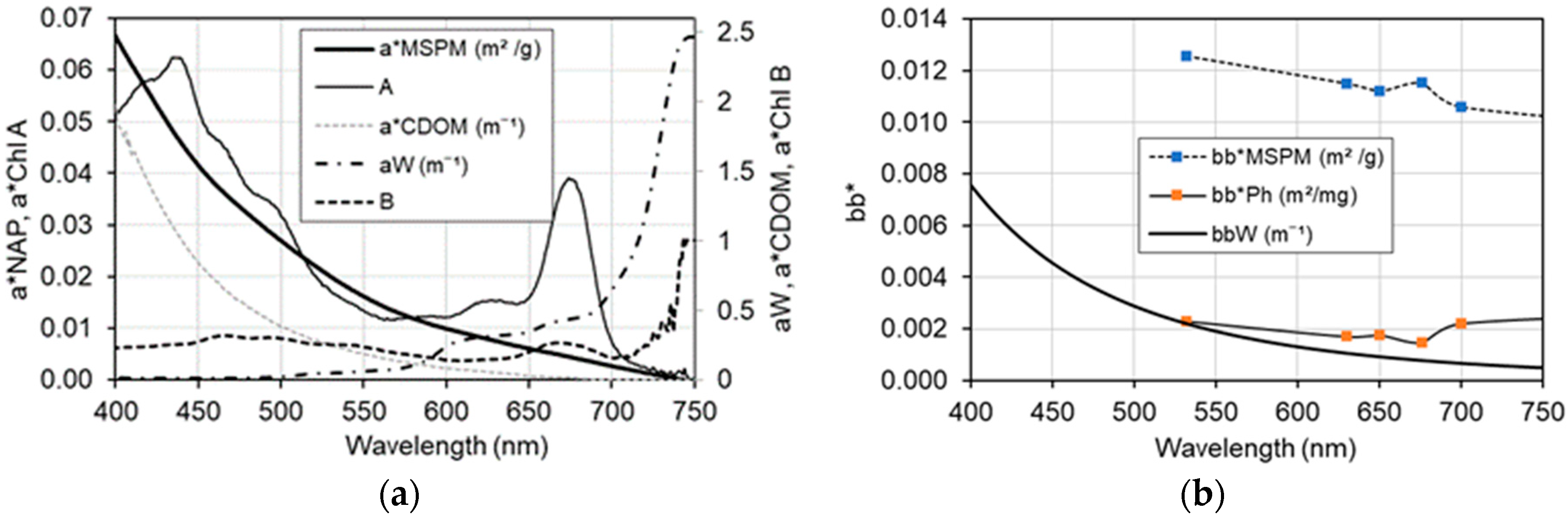
3.1. Inherent Optical Properties

The average concentration-specific absorption and backscatter coefficients for LE and LW are given in Figure 1a,b, respectively. The Chl-a dependent a*Ph (Equation (3)) was defined by the A and B coefficients presented in Figure 1a. Derived a*MSPM and a*CDOM showed the typical exponential increase in absorption towards shorter wavelengths. Absorption spectra were consistent in shape and within the wide-ranging magnitude of previous inland water observations [35,40,43]. Particulate absorption measured in this study were corrected to zero NIR absorption, as has been assumed elsewhere [44,45]; however, it has been suggested that mineral sediments do exhibit significant absorption in the NIR ([46,47,48]). As such, it is possible that the a*MSPM adopted here may result in overestimations in our simulated reflectance, although the effect on simulated MCI is anticipated to be small (for example in turbid and productive water with [Chl-a] at 50 mg/m3 and [MSPM] at 30 g/m3, the simulated MCI difference caused by an increase of a*MSPM at 0.005 m−1 is 6.8%). Average bb*MSPM were comparable with observations of [49] and [50] but somewhat lower than reported in [43]. The magnitude and spectral shape of bb*Ph derived here fell within the range of observations from phytoplankton cultures measured by [51] and [52]. Spectral bb*Ph showed elevated backscatter at wavelengths greater than 700 nm, consistent with observations of gas vacuolate cyanobacteria [52,53,54], which are known to be prevalent in LW and LE. Small depressions in the bb*MSPM may be due to the anomalous dispersion effects due to the strong absorption features of chlorophyll-a [55] and are likely artifacts of the statistical partitioning of organic and inorganic backscatter.

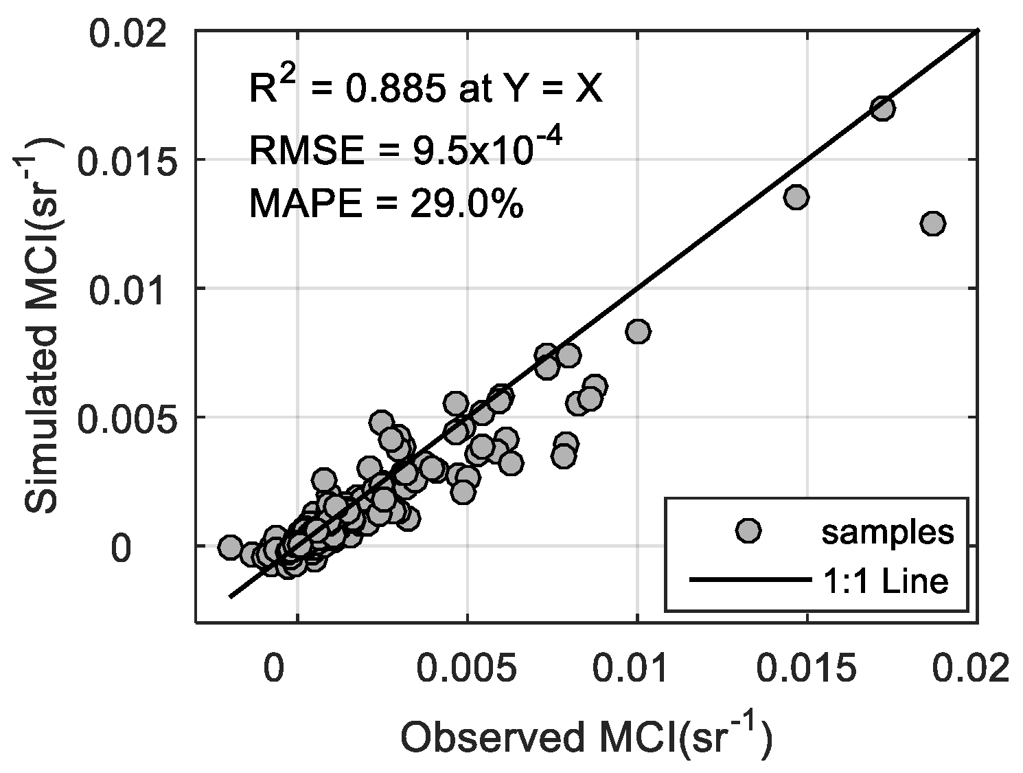
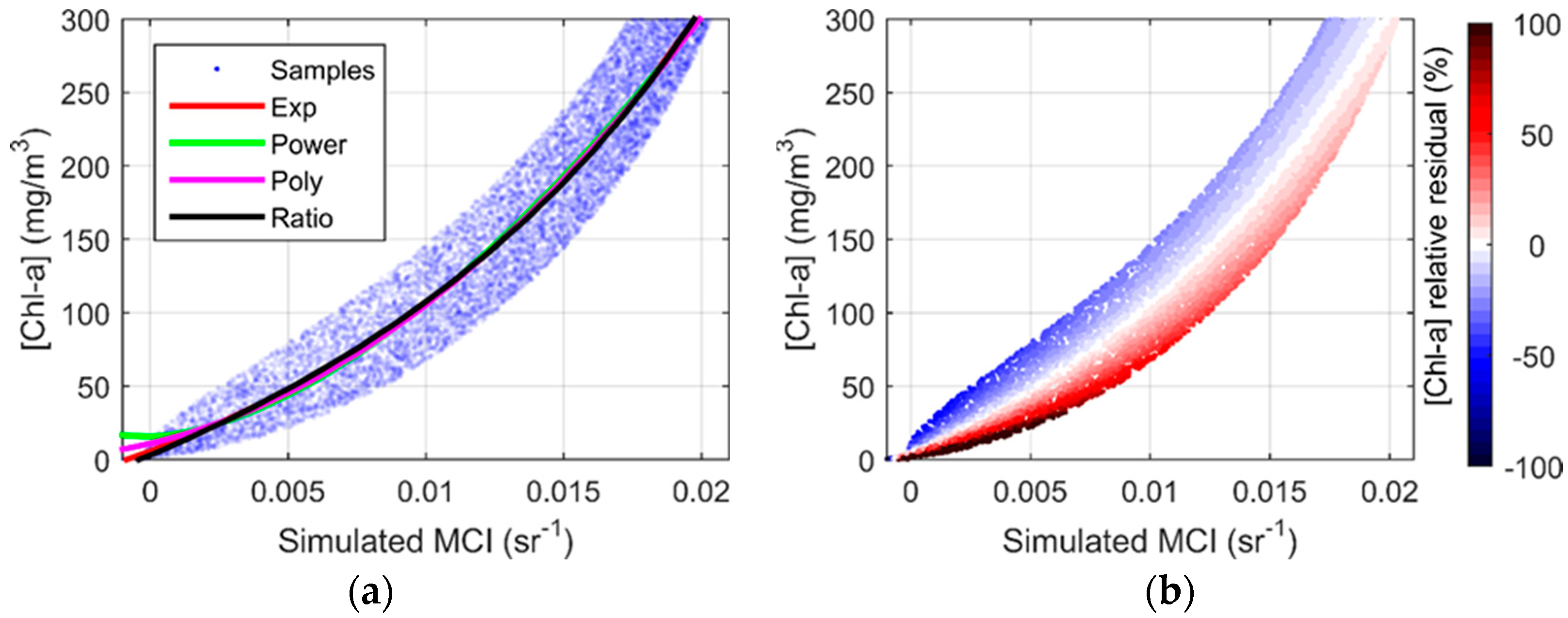
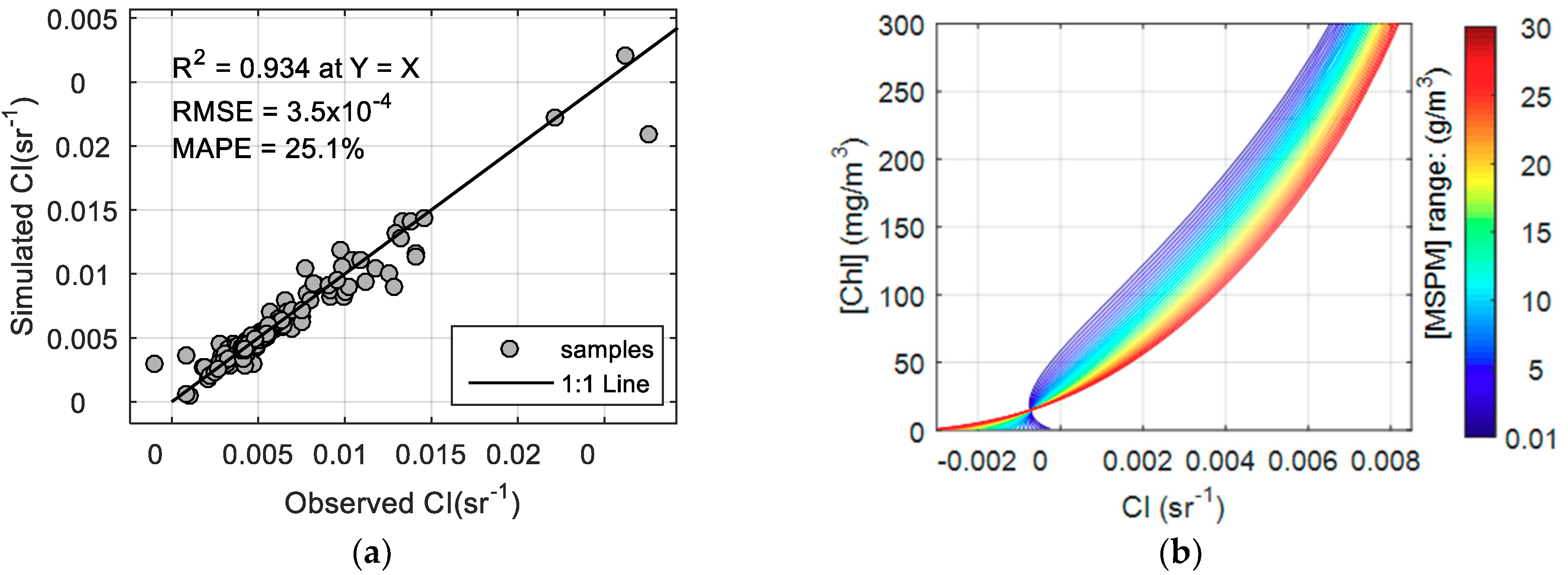
3.2. MCI Simulation and Validation

To evaluate the agreement between in situ samples and the Ecolight modelling described in Section 2.3, measured SIOPs and water constituents (Table 1, Figure 1) were used to simulate spectral Rrs between 600 nm and 885 nm at 5 nm increments and, subsequently, compute MCI for all stations. Ecolight-simulated MCI agreed well with MCI calculated on in situ measured Rrs (R2 = 0.885, RMSE = 9.5 × 10⁻⁴, at Y = X, Figure 2). The strong agreement between measured and modelled indices suggest here that we can have reasonable confidence in the model outcome. Nevertheless, care should be taken to consider various sources of uncertainty when interpreting the model results and in applying this approach to different systems. Figure 2 suggests some systematic underestimation of MCI especially with higher biomass. Model simulations were based on average SIOPs measured in two turbid eutrophic North American lakes and a default Chl-a fluorescence term. It is well known, however, that cyanobacteria have lower Chl-a fluorescence yield than eukaryotic phytoplankton [56], with most of the chlorophyll-a molecules belonging to the non-fluorescing photosystem I (PSI) [57]. In cyanobacteria, phycobiliproteins also contribute to fluorescence, which overlap with the spectrum of chlorophyll emission [58]. Using the default Ecolight fluorescence term may therefore overestimate Rrs at 681 nm, leading to a reduction in simulated MCI as observed here. Enhancing the capabilities of Ecolight to enable multiple fluorescence terms (including phycocyanin) to be more representative of cyanobacteria dominated waters may allow further improvements in the model agreement.
Documented wide variation in IOPs over optically complex inland waters brought about by regional and seasonal differences in the composition of optically active constituents [35,43] may alter the simulations presented here. Variations in phytoplankton community composition in Lake Erie, for example, have been shown to have a significant influence on optical properties and remote sensing Chl-a retrievals [53]. Differences in the spectral properties of IOPs brought about by uncertainties in methodological and/or statistical partitioning of organic and inorganic fractions, may produce additional variability. Furthermore, bias in simulated Rrs may be introduced by non-homogenous vertical distributions of cyanobacterial biomass [59].

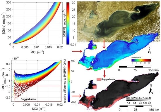
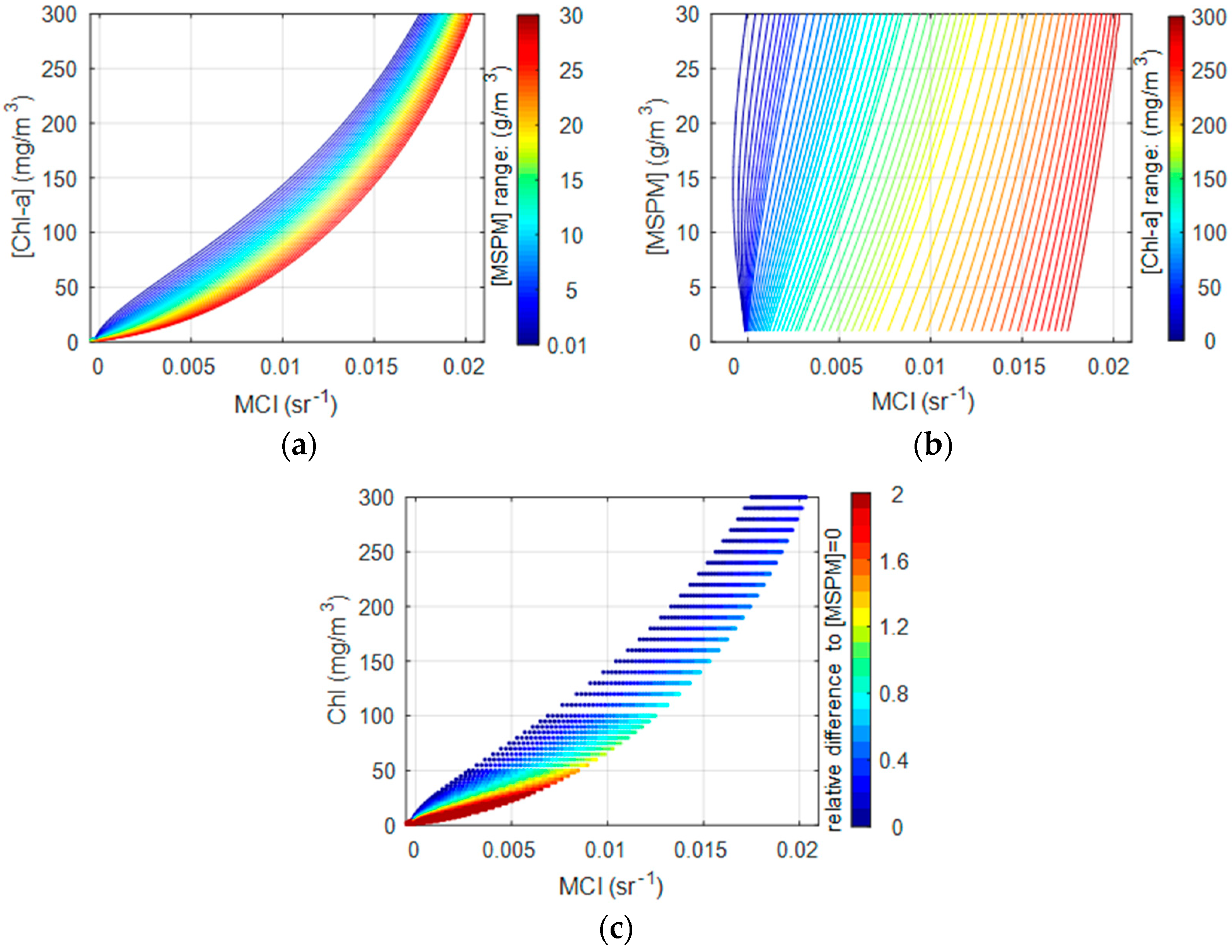
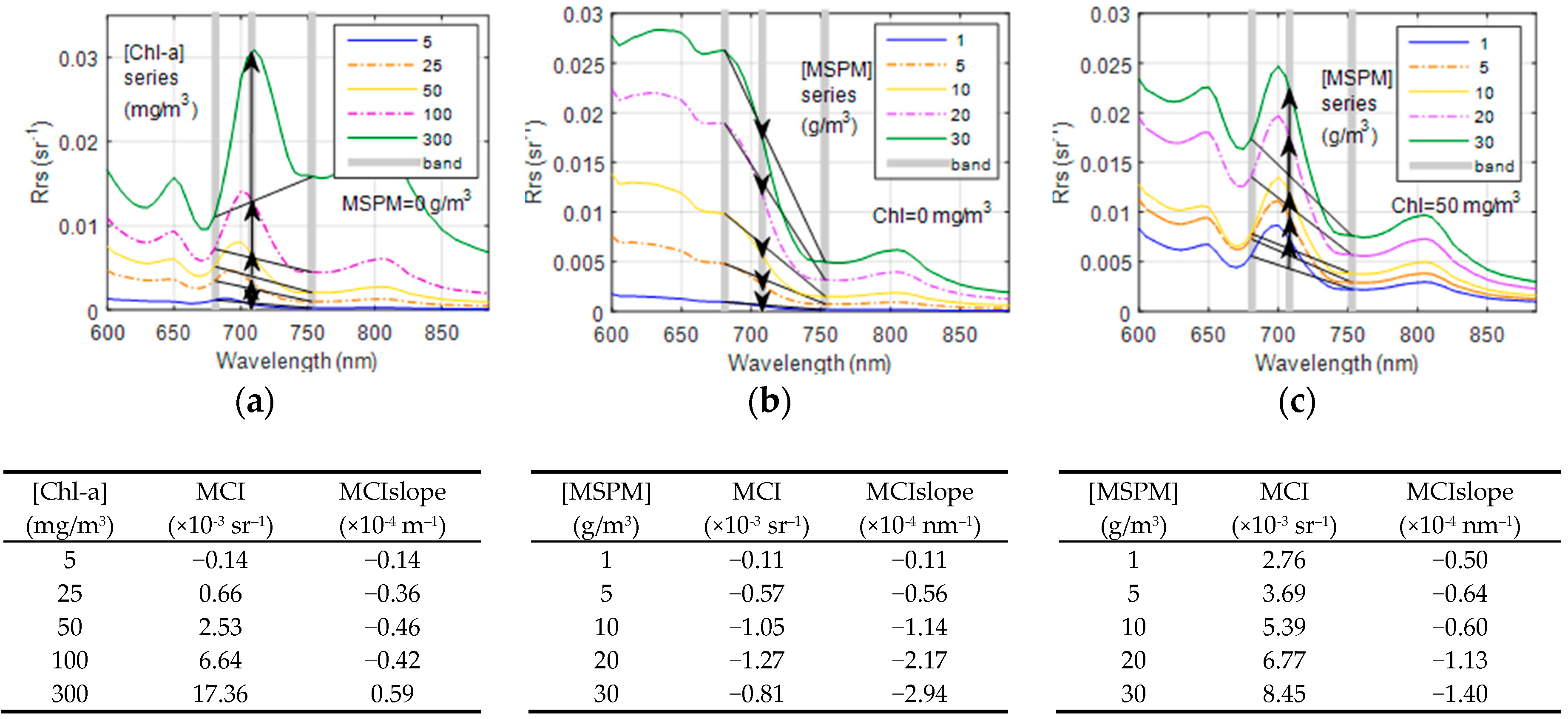
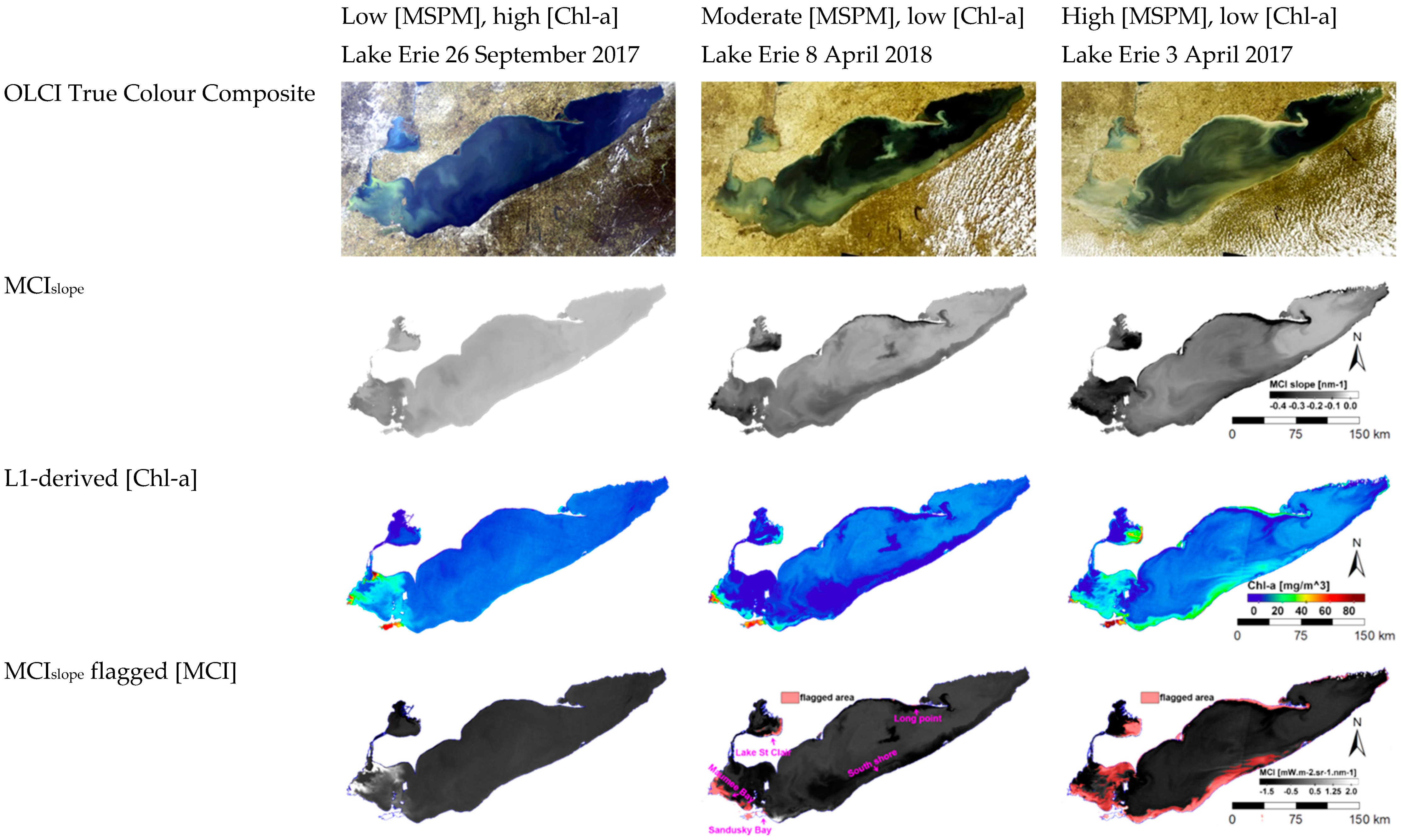
3.3. The Effect of MSPM on Simulated MCI

The MCI derived from simulated Rrs were computed over the [Chl-a] and [MSPM] ranges of 0.1–300 mg/m3 and 0.1–30 g/m3, respectively, consistent with the ranges of these two constituents observed in the field on LW and LE (Table 1). During the simulation, [Chl-a] had increments of 1 in the range 1–10 mg/m3, 2 from 10–30 mg/m3, 3 from 30–50 mg/m3, 5 from 50–100 mg/m3, and 10 from 100–300 mg/m3, while [MSPM] had increments of 1 from 1–30 g/m3. Figure 3a shows a non-linear relationship between simulated MCI and [Chl-a] which tends toward saturation at ~0.02 sr−1 and [Chl-a] ~300 mg/m3. This is in good agreement with in situ observations of [24] from Lake of the Woods over the same [Chl-a] range. The saturation of line-height algorithms is due to the increasing contribution from absorption relative to backscatter with increasing algal/cyanobacterial biomass and the known migration of the fluorescence/backscatter peak toward longer wavelengths. Switching algorithms, such as the MPH, target the changing peak location and aim to extend the sensitivity of Chl-a detection across a broader [Chl-a] range. The series of curves in Figure 3a suggest significant sensitivity of the MCI–[Chl-a] relationship to [MSPM], leading to increases in MCI for any given [Chl-a] due to the effects of a*MSPM and bb*MSPM, which are not spectrally neutral across the MCI wavelength interval (see Figure 1). This variability in the relationship between MCI and [Chl-a] could lead to significant uncertainties in derived Chl-a under turbid water conditions.
When interpreting the impact of MSPM on the MCI–[Chl-a] relationship from another perspective in Figure 3b, increasing [MSPM] results in an increase in MCI at a given [Chl-a], with the exception of very low [Chl-a]. At low [Chl-a] (as indicated by the blue curves in Figure 3b), MCI first decreases and then increases with increasing [MSPM]. The reduction in the slope of the MCI versus [MSPM] relationship with increasing [Chl-a] suggests the impact of MSPM on MCI decreases at high [Chl-a]. Indeed Figure 3c confirms the greatest uncertainty in derived [Chl-a] occurs at [Chl-a] < 50 mg/m3 when [MSPM] is greater than 20 g/m3, with the relative error decreasing substantially for [Chl-a] > 50 mg/m3.

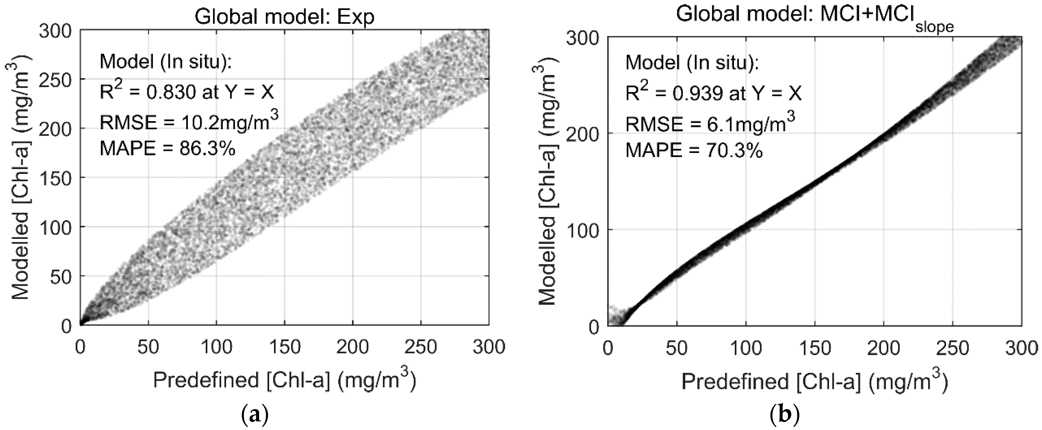
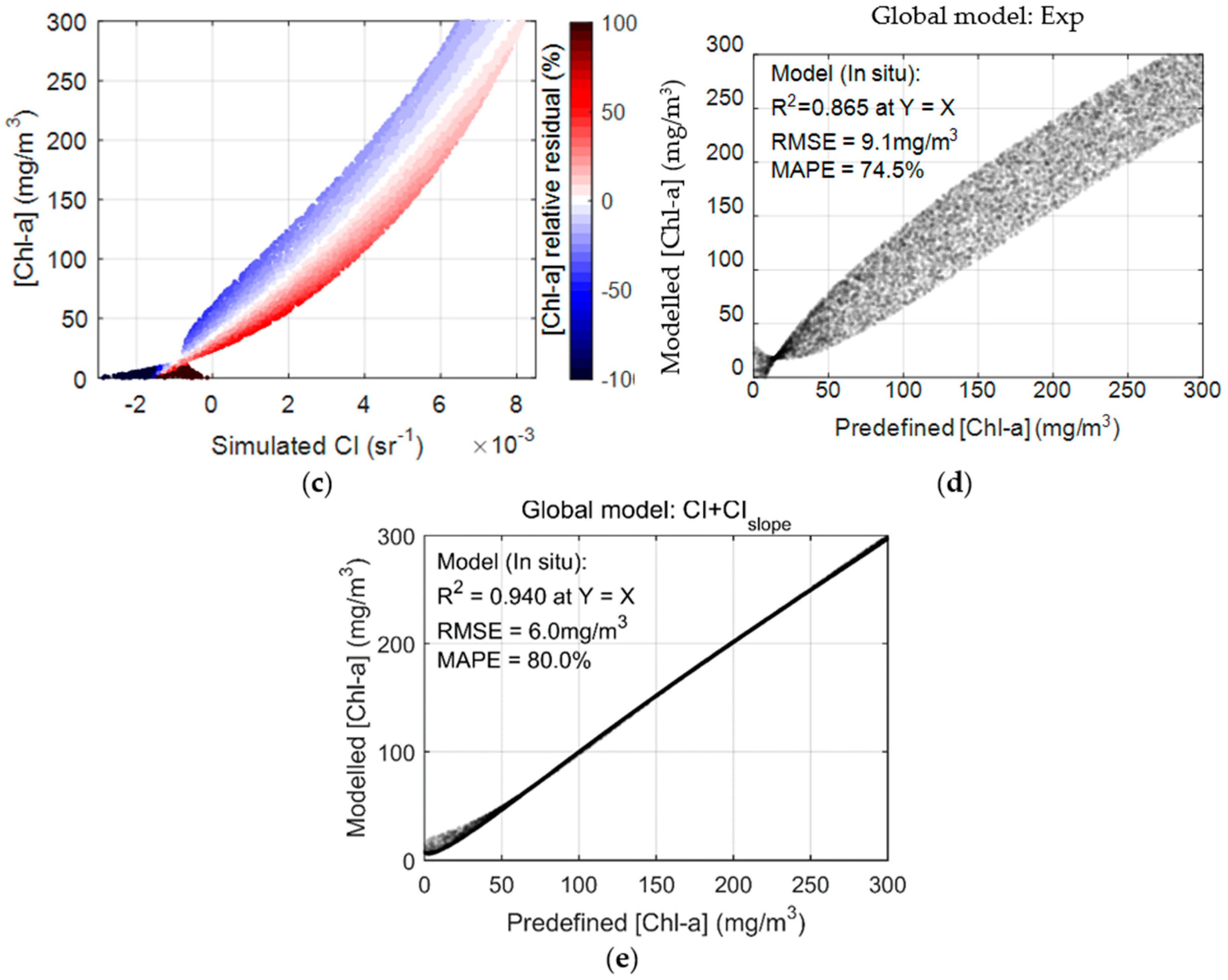
3.4. Global Performance Assessment of [Chl-a] Retrievals

A set of 10,000 Rrs spectra were simulated with randomly varying concentrations of Chl-a and MSPM, approximately uniformly distributed over the ranges 0–300 mg/m3 and 0–30 g/m3 respectively. This dataset provides sufficient samples across the full concentration ranges observed in the field and is used to capture the joint effect of [Chl-a] and [MSPM] on MCI and assess the performance of MCI-retrieved Chl-a from a global fit to the dataset. The large population size makes it possible to test the fit of different types of regression models between MCI and Chl-a over a wide [Chl-a] range. Computed MCI were divided randomly into 10 groups for separate regressions, each group with 1000 data points, and then the coefficients and performance metrics were averaged to obtain a stable evaluation of each model fit. A number of model forms were tested to fit the MCI–[Chl-a] distribution (Figure 4a, Table 2); exponential, power, polynomial, and rational polynomial functions. All the functions fitted the MCI-[Chl-a] distribution similarly well with R2 > 0.92, consistent RMSE of ~23 mg/m3 and MAPE ranging from 25% for the exponential fit to 68% for the power fit. The rational polynomial regression was a variant of a typical first-order rational polynomial, keeping coefficients positive and including an intercept, consistent with the approximate theoretical solution to the MCI-[Chl-a] relationship. Because many published algorithms are based on limited in situ datasets, the relationship between MCI and [Chl-a] and indeed many of the line-height algorithms are often fitted with linear functions over a specific [Chl-a] range [1,4,22], thus this analysis provides evidence of the form of the relationship over a wide range of conditions. Figure 4b shows the resulting MAPE in [Chl-a] derived from the global exponential fit, demonstrating the underestimation of [Chl-a] at low [MSPM] and overestimation at higher [MSPM]. Consistent with Figure 3c, the greatest overestimation occurs at high [MSPM] and [Chl-a] < 50 mg/m3.

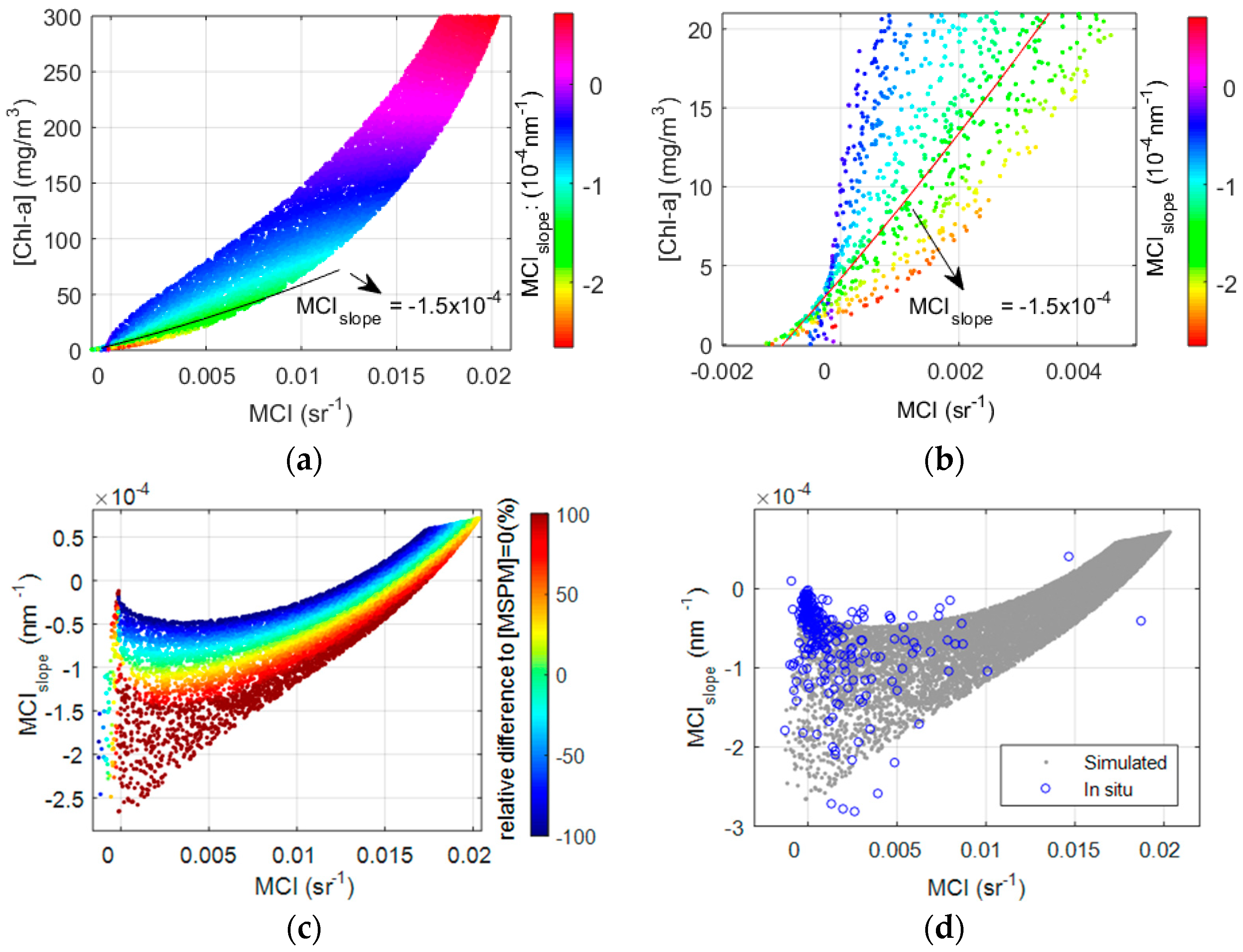
3.5. A Novel Solution for Improved Chl-a Retrievals Using Both MCI and Its Slope

This study explored how to constrain the effect of MSPM on MCI-derived [Chl-a] using the additional spectral information of the slope of the MCI baseline. MCIslope is defined according to Equation (8).
M C I s l o p e = R r s λ m a x R r s λ m i n λ m a x λ m i n
Figure 5a shows that under conditions of variable algal/cyanobacterial biomass when [MSPM] = 0, the modeled MCI baseline slope increases positively with increasing [Chl-a]. In contrast, in the absence of Chl-a (Figure 5b), there is no positive MCI under a range of [MSPM] up to 30 g/m3, and the spectral backscatter properties of MSPM lead to an increasingly negative slope of the MCI baseline with increasing [MSPM]. Consequently, under mixed sediment-algae conditions (Figure 5c), increasing [MSPM] leads to the steepening negative slope of the MCI baseline while coincidentally increasing MCI.
Figure 6a shows the variability of MCIslope in the relationship between MCI and [Chl-a] over the range of [MSPM] shown in Figure 3a. As suggested by the individual spectra in Figure 5, MCIslope increases consistently with increasing [Chl-a], to a positive slope above [Chl-a] ~200 mg/m3. For a constant [Chl-a], MCI increases while MCIslope decreases with an increasing contribution from MSPM, with the greatest variability being for [Chl-a] < 50 mg/m3. At very low [Chl-a] (< ~2 mg/m3, Figure 6b), the relationship changes, where MCI decreases with increasing [MSPM] while the MCIslope continues to decrease. Figure 6c shows the distribution of the [Chl-a] residuals relative to modeled [Chl-a] at [MSPM] = 0, showing the large potential retrieval error when MCIslope was < ~−1.5 × 10⁻⁴ nm−1. The low residual errors at MCI < 0 are again the product of the switch in the MCI:[Chl-a] relationship seen in Figure 6b. The MCI and MCIslope measured on in situ Rrs show a distribution consistent with modeling results (Figure 6d).
We propose a novel multiple regression solution incorporating both MCI and MCIslope to reduce the uncertainties in derived [Chl-a] due to the spectral variations in Rrs driven by MSPM. Figure 7a,b show the comparison of [Chl-a] derived from MCI using only an exponential model, and both MCI and MCIslope with a quadratic polynomial model. Model-simulated [Chl-a] (grey points in the figures) show a large variation around the 1:1 line in Figure 7a for the MCI only approach while the combined MCI and MCIslope approach substantially decreases the variation and forces the data closer to the 1:1 line. The combined MCI and MCIslope approach results in a significant reduction in the RMSE in derived [Chl-a], from 23.1 to 5.1 mg/m3 for the simulated dataset and from 10.2 to 6.1 mg/m3 for in situ derived MCI.
One major advantage of line-height algorithms in estimating Chl-a is that they are fairly insensitive to the atmospheric contribution to the TOA remote sensing signal, and relatively robust to atmospheric correction errors. However, that same advantage may not necessarily hold for a combined MCI and MCIslope approach, where the nature of the slope determination may be more sensitive to spectral atmospheric correction uncertainties than the line-height measure alone as well as errors propagated. This study has demonstrated the potential of using line-height measures and their baseline slopes to refine Chl-a retrieval algorithms using both in situ and modeled Rrs. Where atmospheric correction over optically complex inland and coastal waters results in a reliable level-2 spectral Rrs product, this approach may indeed provide enhanced Chl-a retrievals. However, due to the remaining challenges in atmospheric correction over highly turbid waters, as well as the successful application of line-height algorithms to TOA radiance or BRR products, we propose an alternate approach of using line-height slope parameters to define a quality flag. Slope thresholds would therefore mask potential areas of significant MSPM contamination and reduce the risk of erroneously high [Chl-a] and potential false positive algal bloom detection. A threshold MCIslope of <−1.5 × 10⁻⁴ nm−1, as shown in Figure 6a,b, removes a large fraction of those Chl-a retrievals with high uncertainty due to MSPM contamination, and would limit false positive bloom detection errors while maintaining the advantages and simplicity of an MCI Chl-a retrieval. This threshold may apply to accurate atmospheric-corrected Rrs products, but alternate thresholds are required for TOA radiance and/or BRR products. Furthermore, it is not yet known how a threshold might vary regionally depending on IOP variability; further work is required to confirm the stability and widespread applicability of a single threshold.
Three example level-1 OLCI scenes of Lake Erie are presented in Figure 8, from 26 September 2017, 8 May 2018, and 3 May 2017, capturing conditions of minimal sediment loads during a late summer algal bloom, moderate mineral resuspension with low [Chl-a], and heavy mineral resuspension with low [Chl-a], respectively. Average wind speeds at Windsor Airport, Ontario, over the 24 h prior to image capture were 2, 2.5, and 6.3 m/s, respectively, suggesting increasing sediment resuspension potential. True colour images in May of both years show areas of high near-shore mineral turbidity, for example, along the north shores (erosion of cohesive bluffs which contribute to the formation of the Long Point spit, [60]) as well as the shallow west basin and Lake St, Clair. The image of 8 May 2018 demonstrates the MCI’s tolerance of moderate mineral turbidity, resulting in no positive bias in the MCI-derived [Chl-a], but instead suggesting reduced [Chl-a] in turbidity zones, consistent with the modeled underestimation of [Chl-a] at low to moderate [MSPM] and low [Chl-a]. With increasing sediment, however, the switch evident in the modeling results is also demonstrated in imagery, where the heavy sediment loads of 3 May 2017 lead to falsely elevated MCI-derived [Chl-a]. Mapped MCIslope for each day can be seen to decrease from the predominantly algal conditions of September 2017 to the sediment-laden image of May 2017. Applying a flag threshold to OLCI level-1 products of MCI > 0 mW m–2 sr−1 nm−1 and MCIslope < −0.3 nm−1 accurately masks those areas of potential sediment contamination and false positive blooms while preserving reliable Chl-a retrievals (Figure 8).

3.6. Applicability to Other Line-Height Algorithms

In addition to the MCI, there are many similar R-NIR line-height-based algorithms such as the fluorescence line height (FLH) [18], cyanobacteria index (CI) [17], and maximum peak height (MPH) [2], which may benefit from this approach to minimizing Chl-a retrieval uncertainties due to the presence of mineral sediments. Similar to the MCI, they are often applied in turbid waters under the assumption of insensitivity to mineral scattering. Here, for example, we present a comparable analysis of the CI, which measures the spectral shape of Rrs centered at 681 nm with bands at 665 nm and 709 nm forming the baseline [17]. The effect of MSPM on CI is consistent with that of the MCI (Figure 9), creating the potential for significant overestimates in CI-derived [Chl-a] in turbid waters. Like Figure 2, Figure 4, and Figure 7 for the MCI, Figure 9 provides the corresponding evaluation of the CI, which is very similar in many aspects to the MCI, including performing a satisfactory model simulation (Figure 9a), having a general variation in magnitude and shape of the CI:[Chl-a] relationship caused by [MSPM] (Figure 9b), and in the magnitude and distribution of the MAPE residual (Figure 9c). Consistent with the results from the MCI, a combined CI and CIslope approach results in a considerable improvement in Chl-a retrievals, with reductions in the RMSE in derived [Chl-a], from 22.2 to 2.2 mg/m3 for the simulated dataset and from 9.3 to 6.0 mg/m3 for in situ derived CI. Of note in Figure 9b and in agreement with observations for the MCI is the reversal of the CI:[Chl-a] relationship with MSPM at low [Chl-a], whereby MSPM at first causes a decrease in CI before increasing. This common feature suggests the unlikely occurrence of false positive bloom reports due to the low to moderate [MSPM] at low [Chl-a] using CI- or MCI-based algorithms. The OLCI images comparable to Figure 8 (not shown) suggest extreme sediment loads are also likely to cause erroneous CI-retrieved [Chl-a]. Like the MCI, variability in SIOPs used would result in some variability in the model outcomes, notably in the width of the CI range and the location of the inflection point, although the general trends would remain consistent.

4. Summary and Conclusions

This study investigated the potential impact of MSPM on chlorophyll-a concentrations as derived from red/near-infrared line-height algorithms, such as the MCI and CI—approaches widely used in the detection of algal blooms in turbid coastal and inland waters. Remote sensing reflectance was simulated using the radiative transfer model Ecolight, with resulting line-height indices (MCI and CI) agreeing well with in situ observations. Modelled spectral Rrs showed significant sensitivity to mineral sediments in the R-NIR range. At very low Chl-a (< ~2 mg/m3), model results and image observations suggest that false positive algal bloom reports are unlikely for MSPM < ~20g/m3 (in fact, MCI and CI are inversely related to MSPM when Chl-a = 0 and imagery confirmed decreased MCI in moderate turbidity zones). For higher Chl-a, and/or heavily sediment laden waters with low Chl-a, the model results suggest MCI and CI are significantly enhanced by MSPM. Under conditions of mixed algal/mineral turbidity, as might be expected during wind-mixed conditions in shallow lakes (when cyanobacteria may be vertically uniform throughout the water column and sediment re-suspended from the bottom), Chl-a may be overestimated by these algorithm approaches. Wind events have been shown to lead to significant reductions in satellite-detected Chl-a due to the mixing of the surface algal biomass [61,62]. Results of the present study may further complicate the interpretation of satellite observations during wind events due to the potential for overestimated Chl-a caused by scattering-enhanced algal indices.
The MSPM had measurable effects on the baseline slope of the MCI and CI, which forms the basis of a novel approach for reducing uncertainties in satellite-derived Chl-a in turbid waters. Combining both MCI and its baseline slope parameter MCIslope (or CI and CIslope) resulted in considerable improvements to Chl-a retrieval accuracies compared with using the MCI (or CI) alone. Even if line-height slope parameters are not used to directly correct derived Chl-a, they can be used effectively as a method of flagging potentially erroneous Chl-a retrievals suspected of being contaminated by MSPM. Flag thresholds may be set on the basis of empirical evidence for both atmospherically and non-atmospherically corrected imagery. Quality flags based on a threshold MCIslope were able to accurately delineate those areas of OLCI imagery where MSPM led to erroneously high Chl-a retrievals to effectively limit false positive bloom reports.
For very high Chl-a concentrations, the model results suggest continued sensitivity to MSPM, although relative errors were reduced. However, under intense algal bloom conditions, particularly under quiescent conditions, increased buoyancy of cyanobacteria can lead to surface scums or cyanobacterial mats. Under such circumstances, a pure algal/cyanobacterial signal can typically be assumed, as the satellite-measured MCI will originate only from the surface biomass and not the potentially MSPM-laden water below it, therefore reducing the likelihood of large MSPM-induced algorithm uncertainties under surface bloom conditions.
The model results are dependent on the predefined IOPs and, thus, may vary regionally and seasonally depending on the composition of the main water colouring constituents. Any defined flag thresholds therefore require further validation, and if necessary, tuning to fit various level-1 and level-2 radiance or reflectance products, and which is the focus of ongoing research, but at present, the approach appears promising in its potential for improved Chl-a retrievals in turbid waters.

Author Contributions

The study was conceptualized by C.B., methodology developed and validated by C.Z., and results interpreted by C.Z. and C.B. Original draft preparation and writing was completed by C.Z. and reviewed and edited by C.B.

Funding

This study was funded by Environment and Climate Change Canada under the Lake Winnipeg Basin Initiative and the Great Lakes Protection Initiative.

Acknowledgments

The authors would like to thank the Lake Winnipeg Research Consortium and Canadian Coastguard for access to the RV Namao and CCGS Limnos. The OLCI data were acquired from the Copernicus open access sentinel hub.

Conflicts of Interest

The authors declare no conflict of interest.

References

  1. Binding, C.E.; Greenberg, T.A.; McCullough, G.; Watson, S.B.; Page, E. An analysis of satellite-derived chlorophyll and algal bloom indices on Lake Winnipeg. J. Great Lakes Res. 2018, 44, 436–446. [Google Scholar] [CrossRef]
  2. Matthews, M.W.; Bernard, S.; Robertson, L. An algorithm for detecting trophic status (chlorophyll-a), cyanobacterial-dominance, surface scums and floating vegetation in inland and coastal waters. Remote Sens. Environ. 2012, 124, 637–652. [Google Scholar] [CrossRef]
  3. Stumpf, R.P.; Wynne, T.T.; Baker, D.B.; Fahnenstiel, G.L. Interannual Variability of Cyanobacterial Blooms in Lake Erie. PLoS ONE 2012, 7, e42444. [Google Scholar] [CrossRef] [PubMed]
  4. Palmer, S.C.J.; Hunter, P.D.; Lankester, T.; Hubbard, S.; Spyrakos, E.; Tyler, A.N.; Présing, M.; Horváth, H.; Lamb, A.; Balzter, H.; et al. Validation of Envisat MERIS algorithms for chlorophyll retrieval in a large, turbid and optically-complex shallow lake. Remote Sens. Environ. 2015, 157, 158–169. [Google Scholar] [CrossRef] [Green Version]
  5. Kling, H.J. A summary of past and recent plankton of Lake Winnipeg, Canada using algal fossil remains. J. Paleolimnol. 1998, 19, 297–307. [Google Scholar] [CrossRef]
  6. Pick, F.R. Blooming algae: A Canadian perspective on the rise of toxic cyanobacteria. Can. J. Fish. Aquat. Sci. 2016, 73, 1149–1158. [Google Scholar] [CrossRef]
  7. Watson, S.B.; Ridal, J.; Boyer, G.L. Taste and odour and cyanobacterial toxins: Impairment, prediction, and management in the Great Lakes. Can. J. Fish. Aquat. Sci. 2008, 65, 1779–1796. [Google Scholar] [CrossRef]
  8. Winter, J.G.; DeSellas, A.M.; Fletcher, R.; Heintsch, L.; Morley, A.; Nakamoto, L.; Utsumi, K. Algal blooms in Ontario, Canada: Increases in reports since 1994. Lake Reserv. Manag. 2011, 27, 107–114. [Google Scholar] [CrossRef] [Green Version]
  9. Odermatt, D.; Gitelson, A.; Brando, V.E.; Schaepman, M. Review of constituent retrieval in optically deep and complex waters from satellite imagery. Remote Sens. Environ. 2012, 118, 116–126. [Google Scholar] [CrossRef] [Green Version]
  10. O’Reilly, J.E.; Maritorena, S.; Mitchell, B.G.; Siegel, D.A.; Carder, K.L.; Garver, S.A.; Kahru, M.; McClain, C. Ocean color chlorophyll algorithms for SeaWiFS. J. Geophys. Res. Ocean. 1998, 103, 24937–24953. [Google Scholar] [CrossRef] [Green Version]
  11. Antoine, D.; d’Andon, F.; Bourg, L. Sentinel-3 optical products and algorithm definition. In OLCI Level 2 Algorithm Theoretical Basis Document: Ocean Color Products in Case 1 Waters; ACRI ST: Cannes, France, 2010. [Google Scholar]
  12. Carder, K.L.; Chen, F.R.; Lee, Z.P.; Hawes, S.K.; Kamykowski, D. Semianalytic Moderate-Resolution Imaging Spectrometer algorithms for chlorophyll a and absorption with bio-optical domains based on nitrate-depletion temperatures. J. Geophys. Res. Ocean. 1999, 104, 5403–5421. [Google Scholar] [CrossRef]
  13. Dall’Olmo, G.; Gitelson, A.A.; Rundquist, D.C. Towards a unified approach for remote estimation of chlorophyll-a in both terrestrial vegetation and turbid productive waters. Geophys. Res. Lett. 2003, 30. [Google Scholar] [CrossRef]
  14. Gower, J.; King, S.; Borstad, G.; Brown, L. Detection of intense plankton blooms using the 709 nm band of the MERIS imaging spectrometer. Int. J. Remote Sens. 2005, 26, 2005–2012. [Google Scholar] [CrossRef]
  15. Gons, H.J. Optical Teledetection of Chlorophyll a in Turbid Inland Waters. Environ. Sci. Technol. 1999, 33, 1127–1132. [Google Scholar] [CrossRef]
  16. Le, C.; Li, Y.; Zha, Y.; Sun, D.; Huang, C.; Lu, H. A four-band semi-analytical model for estimating chlorophyll a in highly turbid lakes: The case of Taihu Lake, China. Remote Sens. Environ. 2009, 113, 1175–1182. [Google Scholar] [CrossRef]
  17. Wynne, T.T.; Stumpf, R.P.; Tomlinson, M.C.; Warner, R.A.; Tester, P.A.; Dyble, J.; Fahnenstiel, G.L. Relating spectral shape to cyanobacterial blooms in the Laurentian Great Lakes. Int. J. Remote Sens. 2008, 29, 3665–3672. [Google Scholar] [CrossRef]
  18. Letelier, R.M.; Abbott, M.R. An analysis of chlorophyll fluorescence algorithms for the moderate resolution imaging spectrometer (MODIS). Remote Sens. Environ. 1996, 58, 215–223. [Google Scholar] [CrossRef]
  19. Philpot, W.D. The derivative ratio algorithm: Avoiding atmospheric effects in remote sensing. IEEE Trans. Geosci. Remote Sens. 1991, 29, 350–357. [Google Scholar] [CrossRef]
  20. Hu, C.; Lee, Z.; Ma, R.; Yu, K.; Li, D.; Shang, S. Moderate Resolution Imaging Spectroradiometer (MODIS) observations of cyanobacteria blooms in Taihu Lake, China. J. Geophys. Res. Ocean. 2010, 115. [Google Scholar] [CrossRef]
  21. Matthews, M.W.; Odermatt, D. Improved algorithm for routine monitoring of cyanobacteria and eutrophication in inland and near-coastal waters. Remote Sens. Environ. 2015, 156, 374–382. [Google Scholar] [CrossRef]
  22. Tomlinson, M.C.; Stumpf, R.P.; Wynne, T.T.; Dupuy, D.; Burks, R.; Hendrickson, J.; Fulton Iii, R.S. Relating chlorophyll from cyanobacteria-dominated inland waters to a MERIS bloom index. Remote Sens. Lett. 2016, 7, 141–149. [Google Scholar] [CrossRef]
  23. Gower, J.; King, S.; Borstad, G.; Brown, L. The importance of a band at 709 nm for interpreting water-leaving spectral radiance. Can. J. Remote Sens. 2008, 34, 287–295. [Google Scholar] [CrossRef]
  24. Binding, C.E.; Greenberg, T.A.; Bukata, R.P. The MERIS Maximum Chlorophyll Index; its merits and limitations for inland water algal bloom monitoring. J. Great Lakes Res. 2013, 39, 100–107. [Google Scholar] [CrossRef]
  25. Gitelson, A.A.; Dall’Olmo, G.; Moses, W.; Rundquist, D.C.; Barrow, T.; Fisher, T.R.; Gurlin, D.; Holz, J. A simple semi-analytical model for remote estimation of chlorophyll-a in turbid waters: Validation. Remote Sens. Environ. 2008, 112, 3582–3593. [Google Scholar] [CrossRef]
  26. Qi, L.; Hu, C.; Duan, H.; Cannizzaro, J.; Ma, R. A novel MERIS algorithm to derive cyanobacterial phycocyanin pigment concentrations in a eutrophic lake: Theoretical basis and practical considerations. Remote Sens. Environ. 2014, 154, 298–317. [Google Scholar] [CrossRef]
  27. Bresciani, M.; Stroppiana, D.; Odermatt, D.; Morabito, G.; Giardino, C. Assessing remotely sensed chlorophyll-a for the implementation of the Water Framework Directive in European perialpine lakes. Sci. Total Environ. 2011, 409, 3083–3091. [Google Scholar] [CrossRef] [Green Version]
  28. Gitelson, A.A.; Gao, B.-C.; Li, R.-R.; Berdnikov, S.; Saprygin, V. Estimation of chlorophyll-a concentration in productive turbid waters using a Hyperspectral Imager for the Coastal Ocean—the Azov Sea case study. Environ. Res. Lett. 2011, 6, 024023. [Google Scholar] [CrossRef]
  29. Keith, D.J.; Milstead, B.; Walker, H.; Snook, H.; Szykman, J.J.; Wusk, M.; Kagey, L.; Howell, C.; Mellanson, C.; Drueke, C. Trophic status, ecological condition, and cyanobacteria risk of New England lakes and ponds based on aircraft remote sensing. J. Appl. Remote Sens. 2012, 6, 063577. [Google Scholar] [CrossRef]
  30. Mobley, C.D. Light and Water: Radiative Transfer in Natural Waters; Academic Press: San Diego, CA, USA, 1994. [Google Scholar]
  31. Mobley, C.D.; Sundman, L.K.; Sequoia Scientific, Inc. Hydrolight and Ecolight 5.2: Technical Documentation; Sequoia Scientific: Bellevue, WA, USA, 2013. [Google Scholar]
  32. Bunting, L.; Leavitt, P.R.; Simpson, G.L.; Wissel, B.; Laird, K.R.; Cumming, B.F.; St. Amand, A.; Engstrom, D.R. Increased variability and sudden ecosystem state change in Lake Winnipeg, Canada, caused by 20th century agriculture. Limnol. Oceanogr. 2016, 61, 2090–2107. [Google Scholar] [CrossRef]
  33. McCullough, G.K.; Page, S.J.; Hesslein, R.H.; Stainton, M.P.; Kling, H.J.; Salki, A.G.; Barber, D.G. Hydrological forcing of a recent trophic surge in Lake Winnipeg. J. Great Lakes Res. 2012, 38, 95–105. [Google Scholar] [CrossRef]
  34. Mueller, J.L.; Morel, A.; Frouin, R.; Davis, C.; Arnone, R.; Carder, K.; Lee, Z.P.; Steward, R.G.; Hooker, S.; Mobley, C.D.; et al. Ocean Optics Protocols for Satellite Ocean Color Sensor Validation, Revision 4. Volume III: Radiometric Measurements and Data Analysis Protocols; Mueller, J.L., Fargion, G.S., McClain, C.R., Eds.; Goddard Space Flight Space Center: Greenbelt, MD, USA, 2003. [Google Scholar]
  35. Binding, C.E.; Jerome, J.H.; Bukata, R.P.; Booty, W.G. Spectral absorption properties of dissolved and particulate matter in Lake Erie. Remote Sens. Environ. 2008, 112, 1702–1711. [Google Scholar] [CrossRef]
  36. Roesler, C.S. Theoretical and experimental approaches to improve the accuracy of particulate absorption coefficients derived from the quantitative filter technique. Limnol. Oceanogr. 1998, 43, 1649–1660. [Google Scholar] [CrossRef]
  37. SCOR/UNESCO. Determination of Photosynthetic Pigments; Report of SCOR/UNESCO Working Group 17; UNESCO Monographson Oceanographic Methodology: La Jolla, CA, USA, 1966; Volume 1, pp. 9–15. [Google Scholar]
  38. Pope, R.M.; Fry, E.S. Absorption spectrum (380–700 nm) of pure water. II. Integrating cavity measurements. Appl. Opt. 1997, 36, 8710–8723. [Google Scholar] [CrossRef] [PubMed]
  39. Bricaud, A.; Claustre, H.; Ras, J.; Oubelkheir, K. Natural variability of phytoplanktonic absorption in oceanic waters: Influence of the size structure of algal populations. J. Geophys. Res. Ocean. 2004, 109. [Google Scholar] [CrossRef]
  40. Zhang, Y.; Yin, Y.; Wang, M.; Liu, X. Effect of phytoplankton community composition and cell size on absorption properties in eutrophic shallow lakes: Field and experimental evidence. Opt. Express 2012, 20, 11882–11898. [Google Scholar] [CrossRef]
  41. Bricaud, A.; Morel, A.; Babin, M.; Allali, K.; Claustre, H. Variations of light absorption by suspended particles with chlorophyll a concentration in oceanic (case 1) waters: Analysis and implications for bio-optical models. J. Geophys. Res. Ocean. 1998, 103, 31033–31044. [Google Scholar] [CrossRef]
  42. McKee, D.; Cunningham, A.; Wright, D.; Hay, L. Potential impacts of nonalgal materials on water-leaving Sun induced chlorophyll fluorescence signals in coastal waters. Appl. Opt. 2007, 46, 7720–7729. [Google Scholar] [CrossRef]
  43. Moore, T.S.; Mouw, C.B.; Sullivan, J.M.; Twardowski, M.S.; Burtner, A.M.; Ciochetto, A.B.; McFarland, M.N.; Nayak, A.R.; Paladino, D.; Stockley, N.D.; et al. Bio-optical Properties of Cyanobacteria Blooms in Western Lake Erie. Front. Mar. Sci. 2017, 4, 300. [Google Scholar] [CrossRef]
  44. Babin, M.; Stramski, D. Light absorption by aquatic particles in the near-infrared spectral region. Limnol. Oceanogr. 2002, 47, 911–915. [Google Scholar] [CrossRef]
  45. Babin, M.; Stramski, D. Variations in the mass-specific absorption coefficient of mineral particles suspended in water. Limnol. Oceanogr. 2004, 49, 756–767. [Google Scholar] [CrossRef] [Green Version]
  46. Tassan, S.; Ferrari, G.M. An alternative approach to absorption measurements of aquatic particles retained on filters. Limnol. Oceanogr. 1995, 40, 1358–1368. [Google Scholar] [CrossRef] [Green Version]
  47. Bowers, D.G.; Binding, C.E. The optical properties of mineral suspended particles: A review and synthesis. Estuar. Coast. Shelf Sci. 2006, 67, 219–230. [Google Scholar] [CrossRef]
  48. Röttgers, R.; Dupouy, C.; Taylor, B.B.; Bracher, A.; Woźniak, S.B. Mass-specific light absorption coefficients of natural aquatic particles in the near-infrared spectral region. Limnol. Oceanogr. 2014, 59, 1449–1460. [Google Scholar] [CrossRef] [Green Version]
  49. Neukermans, G.; Loisel, H.; Mériaux, X.; Astoreca, R.; McKee, D. In situ variability of mass-specific beam attenuation and backscattering of marine particles with respect to particle size, density, and composition. Limnol. Oceanogr. 2012, 57, 124–144. [Google Scholar] [CrossRef]
  50. Reynolds, R.A.; Stramski, D.; Neukermans, G. Optical backscattering by particles in Arctic seawater and relationships to particle mass concentration, size distribution, and bulk composition. Limnol. Oceanogr. 2016, 61, 1869–1890. [Google Scholar] [CrossRef] [Green Version]
  51. Whitmire, A.L.; Pegau, W.S.; Karp-Boss, L.; Boss, E.; Cowles, T.J. Spectral backscattering properties of marine phytoplankton cultures. Opt. Express 2010, 18, 15073–15093. [Google Scholar] [CrossRef] [PubMed] [Green Version]
  52. Zhou, W.; Wang, G.; Sun, Z.; Cao, W.; Xu, Z.; Hu, S.; Zhao, J. Variations in the optical scattering properties of phytoplankton cultures. Opt. Express 2012, 20, 11189–11206. [Google Scholar] [CrossRef] [PubMed]
  53. Binding, C.E.; Zastepa, A.; Zeng, C. The impact of phytoplankton community composition on optical properties and satellite observations of the 2017 western Lake Erie algal bloom. J. Great Lakes Res. 2019, 45, 573–586. [Google Scholar] [CrossRef]
  54. Matthews, M.W.; Bernard, S. Characterizing the Absorption Properties for Remote Sensing of Three Small Optically-Diverse South African Reservoirs. Remote Sens. 2013, 5, 4370–4404. [Google Scholar] [CrossRef] [Green Version]
  55. Zaneveld, J.R.V.; Kitchen, J.C. The variation in the inherent optical properties of phytoplankton near an absorption peak as determined by various models of cell structure. J. Geophys. Res. Ocean. 1995, 100, 13309–13320. [Google Scholar] [CrossRef]
  56. Seppälä, J.; Ylöstalo, P.; Kaitala, S.; Hällfors, S.; Raateoja, M.; Maunula, P. Ship-of-opportunity based phycocyanin fluorescence monitoring of the filamentous cyanobacteria bloom dynamics in the Baltic Sea. Estuar. Coast. Shelf Sci. 2007, 73, 489–500. [Google Scholar] [CrossRef]
  57. Mimuro, M.; Fujita, Y. Estimation of chlorophyll a distribution in the photosynthetic pigment systems I and II of the blue-green alga Anabaena variabilis. Biochim. Et Biophys. Acta (BBA)–Bioenerg. 1977, 459, 376–389. [Google Scholar] [CrossRef]
  58. Campbell, D.; Hurry, V.; Clarke, A.K.; Gustafsson, P.; Oquist, G. Chlorophyll fluorescence analysis of cyanobacterial photosynthesis and acclimation. Microbiol. Mol. Biol. Rev. 1998, 62, 667–683. [Google Scholar] [PubMed]
  59. Kutser, T.; Metsamaa, L.; Dekker, A.G. Influence of the vertical distribution of cyanobacteria in the water column on the remote sensing signal. Estuar. Coast. Shelf Sci. 2008, 78, 649–654. [Google Scholar] [CrossRef]
  60. Davidson-Arnott, R.G.D.; Reid, H.E.C. Sedimentary processes and the evolution of the distal bayside of Long Point, Lake Erie. Can. J. Earth Sci. 1994, 31, 1461–1473. [Google Scholar] [CrossRef]
  61. Binding, C.E.; Greenberg, T.A.; Jerome, J.H.; Bukata, R.P.; Letourneau, G. An assessment of MERIS algal products during an intense bloom in Lake of the Woods. J. Plankton Res. 2010, 33, 793–806. [Google Scholar] [CrossRef] [Green Version]
  62. Wynne, T.T.; Stumpf, R.P.; Tomlinson, M.C.; Dyble, J. Characterizing a cyanobacterial bloom in Western Lake Erie using satellite imagery and meteorological data. Limnol. Oceanogr. 2010, 55, 2025–2036. [Google Scholar] [CrossRef] [Green Version]
Figure 1. The average concentration-specific inherent optical properties (SIOPs) used in Ecolight for reflectance simulations: (a) concentration-specific absorption coefficients, a*, and (b) concentration-specific backscatter coefficients, bb*. A and B in (a) are coefficients of a*Ph defined in Equation (3).
Remotesensing 11 02306 g001
Figure 2. Comparison of in situ and Ecolight simulated MCI. N = 246, as described in Table 1.
Remotesensing 11 02306 g002
Figure 3. The impact of MSPM on the MCI-[Chl-a] relationship. (a) MCI-[Chl-a] relationship from simulated Rrs; each isoline indicating a constant [MSPM] in the range of 0.1 to 30 g/m3 according to the colored legend. (b) [MSPM]-MCI relation with a [Chl-a] colored legend, and (c) [Chl-a] residuals relative to the MCI:[Chl-a] relationship at [MSPM] = 0.
Remotesensing 11 02306 g003
Figure 4. (a) Ten thousand simulated MCI based on variable [Chl-a] and [MSPM] with global best-fit relationships, also reported in Table 2. (b) Distribution of modelled [Chl-a] residual (MAPE) by applying the exponential fitting in (a).
Remotesensing 11 02306 g004
Figure 5. Modeled reflectance spectra and derived MCI and MCIslope for (a) varying [Chl-a] in the absence of MSPM, (b) varying [MSPM] in the absence of Chl-a, and (c) [Chl-a] = 50 mg/m3 and increasing [MSPM], showing the effect of MSPM on baseline slopes.
Remotesensing 11 02306 g005
Figure 6. (a) The variability of the MCIslope in the relationship between [Chl-a] and MCI and (b) the same variability of the MCIslope in the relationship between [Chl-a] and MCI expanded to show in detail [Chl-a] < 20 mg/m3. (c) The distribution of the [Chl-a] residual relative to derived [Chl-a] at [MSPM] = 0, in the [MCI, MCIslope] space, and (d) in situ derived MCI and MCIslope superimposed over simulated values.
Remotesensing 11 02306 g006
Figure 7. Comparison of global [Chl-a] fitting using (a) only MCI and (b) both MCI and its slope. The regression model used in (a) is the best performance model (exponential) in Table 2. The regression model in (b) is a quadratic polynomial regression from MCI and its slope to [Chl-a].
Remotesensing 11 02306 g007
Figure 8. Three examples of the ocean and land colour instrument (OLCI) scenes showing an RGB true colour composite, MCIslope, L1 MCI-derived [Chl-a], MCIslope mask area overlaid on MCI, using MCI > 0 mW/(m2∙sr∙nm) and MCIslope < −0.15 nm−1.
Remotesensing 11 02306 g008
Figure 9. (a) Comparison of in situ and Ecolight simulated CI, (b) modeled variability of the CI:[Chl-a] relationship in response to MSPM, (c) the distribution of MAPE residual when applying an exponential CI:[Chl-a] best-fit model, (d) modeled and in situ [Chl-a] from a global best-fit regression, and (e) modeled [Chl-a] from combined CI and CIslope regression.
Remotesensing 11 02306 g009aRemotesensing 11 02306 g009b
Table 1. A summary of in situ optical and water quality parameters from lakes Erie (LE) and Winnipeg (LW).
# ObservationsWater ConstituentConcentration
MEANMINMAXSD
LEWater372Chl-a (mg/m3)13.10.516120.4
IOPs292MSPM (g/m3)4.30.0124.75.1
Rrs138aCDOM(440) (m−1)0.40.032.40.4
LWWater316Chl-a7.60.829024.6
IOPs209MSPM7.00.0131.66.6
Rrs108aCDOM(440)1.80.265.50.8
Note: IOPs: inherent optical properties; MSPM: mineral suspended particulate matter.
Table 2. Comparison of different theoretical models for the relationship between [Chl-a] and MCI. Note that MCI was multiplied by 103 for the coefficients below.
Model (Chl=)abcR2RMSE (mg/m3)MAPE (%)
a · e b · M C I + c 1030.0685−96.80.92823.125.5
a · M C I b + c 1.931.6715.70.92823.168.2
a · M C I 2 + b × M C I + c 0.514.34110.9292339.9
a · M C I / ( b M C I ) + c 33241.83.090.92823.232.1

