Climate Data Records of Vegetation Variables from Geostationary SEVIRI/MSG Data: Products, Algorithms and Applications

Abstract

The scientific community requires long-term data records with well-characterized uncertainty and suitable for modeling terrestrial ecosystems and energy cycles at regional and global scales. This paper presents the methodology currently developed in EUMETSAT within its Satellite Application Facility for Land Surface Analysis (LSA SAF) to generate biophysical variables from the Spinning Enhanced Visible and InfraRed Imager (SEVIRI) on board MSG 1-4 (Meteosat 8-11) geostationary satellites. Using this methodology, the LSA SAF generates and disseminates at a time a suite of vegetation products, such as the leaf area index (LAI), the fraction of the photosynthetically active radiation absorbed by vegetation (FAPAR) and the fractional vegetation cover (FVC), for the whole Meteosat disk at two temporal frequencies, daily and 10-days. The FVC algorithm relies on a novel stochastic spectral mixture model which addresses the variability of soils and vegetation types using statistical distributions whereas the LAI and FAPAR algorithms use statistical relationships general enough for global applications. An overview of the LSA SAF SEVIRI/MSG vegetation products, including expert knowledge and quality assessment of its internal consistency is provided. The climate data record (CDR) is freely available in the LSA SAF, offering more than fifteen years (2004-present) of homogeneous time series required for climate and environmental applications. The high frequency and good temporal continuity of SEVIRI products addresses the needs of near-real-time users and are also suitable for long-term monitoring of land surface variables. The study also evaluates the potential of the SEVIRI/MSG vegetation products for environmental applications, spanning from accurate monitoring of vegetation cycles to resolving long-term changes of vegetation.

1. Introduction

Observations and monitoring are essential components of Global Framework for Climate Services initiative [1,2] that contribute significantly to meet the needs of climate research services. The role that satellites have played in observing the variability and change of the Earth system has increased significantly in the last decades. Thanks to the Earth observation (EO) satellite systems, a large number of variables related to the atmosphere, oceanic and terrestrial domains are accessible [3].

The Satellite Application Facility (SAF) for Land Surface Analysis (LSA) is a leading center for development and operational retrieval of land surface variables from European Organization for the Exploitation of Meteorological Satellites (EUMETSAT), specifically aimed to understand and quantify terrestrial processes and land-atmosphere interactions. Land surface models’ assessment and improvement of high quality and robust EO products are among the target applications of LSA SAF products. Particularly, the geostationary Spinning Enhanced Visible and Infrared Imager (SEVIRI) on board the Meteosat Second Generation (MSG) platform provides a very high temporal resolution (15 minutes) required for resolving the diurnal cycles of radiation, surface albedo and surface temperature [4]. The MSG program covers a series of four identical satellites MSG 1-4 (Meteosat 8-11) launched in 2002, 2005, 2012, and 2015 respectively. SEVIRI operates in 12 spectral channels [5], although only channels 1 (VIS0.6), 2 (VIS0.8) and 3 (NIR1.6), centered at about 0.635 μm (red), 0.81 μm (NIR) and 1.64 μm (SWIR), respectively situate in the optical domain.

The LSA SAF provides also variables for the characterization of terrestrial ecosystems and their role in the energy balance of Earth, such as land surface fluxes and three important biophysical variables related with the amount, structure and state of vegetation: Leaf Area Index (LAI), Fraction of Absorbed Photosynthetically Active Radiation (FAPAR) and Fractional Vegetation Cover (FVC) [6]. These variables are widely used in many land-surface vegetation, climate, and crop production models [7,8,9,10,11,12,13]. FVC represents the fraction of green vegetation covering a unit area of horizontal soil, corresponding to the gap fraction in the nadir direction. LAI is a measure of the amount of live foliage present in the canopy per unit ground surface. The FAPAR is the fraction of photosynthetically active radiation (400-700 nm) absorbed by the green parts of the canopy, and therefore constitutes an indicator of the presence, health and productivity of live vegetation.

Nowadays, consistent long-term data records of these variables with well-characterized uncertainty are currently required by the scientific community to model terrestrial ecosystems and energy cycles at regional and global scales [14]. Models related with land surface and climate usually require Near-Real-Time (NRT) datasets of these variables at high temporal frequencies, and with regional to global coverage [15]. Both, LAI and FAPAR are recognized as essential climate variables in the terrestrial domain by Global Climate Observing System (GCOS) [16].

Several methods have been proposed for estimating biophysical parameters from large scale optical sensors, some of which have been implemented in operational processing lines from POLarization and Directionality of Earth Reflectances (POLDER) [17], Moderate Resolution Imaging Spectroradiometer (MODIS) [18], MISR (Multi-angle Imaging SpectroRadiometer) [19], MEdium Resolution Imaging Spectrometer (MERIS) [20,21], Sea-viewing Wide Field-of-view Sensor (SEAWIFS) [22], VEGETATION [23,24] and Advanced Very High Resolution Radiometer (AVHRR) [25]. These methods can be roughly classified in two main categories: (i) methods based on optimized vegetation indices [26], and (ii) methods based on the inversion of physical models. Both approaches present advantages and drawbacks. It is referred to [27] for a detail intercomparison on the spread of currently available physical models. Although methods that invert physical models can potentially be applied to varying surface types, they require specifying a large number of model parameters, which may lead to unstable solutions [28]. Most inversion methods use one-dimensional (turbid) models (e.g., PROSAIL [29]), thereby assuming surface homogeneity within an image pixel. They are thus limited to address the sub-pixel mixing of land cover types, which is common at coarse resolutions satellites. The process of identifying the sub-pixel proportions of the constituent components is called spectral mixture model (SMM). SMM approaches are methods especially adequate for global studies, since the spatial variability within pixel is high [30,31].

In this paper, we describe the methodology currently used in LSA SAF to operationally generate the suite of SEVIRI/MSG (FVC, LAI and FAPAR) vegetation products. The high frequency of acquisition provided by the SEVIRI instrument assures the availability of cloud-free data for appropriately monitoring the vegetation dynamics in large regions. When one is choosing a retrieval method, one needs to consider the limited spatial and spectral resolution of SEVIRI instrument (i.e., only 3 optical channels and a spatial resolution of 3 km at the sub-satellite point that declines rapidly at higher latitudes). Furthermore, the challenges that the MSG geostationary satellite poses as compared to polar-orbiting satellite sensors due to diurnal variations in the solar zenith angle need to be considered. The algorithm to retrieve FVC relies on a novel stochastic SMM method, which addresses the large variability of soils and vegetation types using statistical (sum of Gaussian) distributions. The LSA SAF operational scheme to retrieve LAI and FAPAR uses statistical relationships general enough for global applications, proposed by Roujean and Lacaze [16] and Roujean and Bréon [32], respectively.

LSA SAF has been providing in NRT vegetation products (FVC, LAI and FAPAR) at two different time resolutions (daily and 10-days) since 2008 over the geostationary Meteosat disk, covering Europe, Africa, the Middle East and parts of South America. The suite of SEVIRI/MSG vegetation products is freely disseminated to users through LSA SAF website (https://landsaf.ipma.pt). During the different operational phases, these vegetation products have been routinely assessed and some improvements have been made in the upgraded versions. LSA SAF has recently reprocessed the entire MSG archive with the latest version of the several retrieval algorithms in order to obtain a continuous and homogeneous Climate Data Records (CDR) of vegetation products. More than fifteen years (January 2004- present) of homogeneous consistent estimates of FVC, LAI and FAPAR fields are available. The 10-days (FVC, LAI and FAPAR) CDRs are part of the suite of EUMETSAT climate products, which include Fundamental CDRs, Thematic CDRs and Data for operational climate monitoring and are also available from EUMETSAT web page (https://navigator.eumetsat.int/).

The paper presents the following structure. Section 2 is dedicated to describe the algorithms to retrieve FVC, LAI and FAPAR. The suite of LSA SAF SEVIRI/MSG vegetation products are described in Section 3, including expert knowledge and a quality assessment of the consistency between the products. Section 4 provides further insight about the added value and introduces examples of its application in numerous environmental applications.

2. Algorithm Description

2.1. SEVIRI/MSG

The algorithm for retrieving biophysical variables from SEVIRI/MSG data uses as input normalized spectral bidirectional reflectance factor (BRDF) at a fixed angular configuration (i.e., vertical illumination and observation angles of 0°) in order to reduce angular effects. This hotspot geometry leads to a minimum contribution of the shadow proportion and a precise estimation of FVC, coinciding with the complement to unity of the gap fraction at nadir direction [16]. Estimating the FVC with increased sun zenith angles would lead to an overestimation of FVC. The main drawback of this geometry is the significant contribution of illuminated soil background, which constitutes a confounding factor for the retrieval of FVC. Figure 1 outlines the main ingredients for deriving the SEVIRI/MSG products including the stochastic SMM approach for retrieving FVC, a pragmatic method for LAI retrieval from FVC, and a method based on an optimized vegetation index for FAPAR determination.

The BRDF algorithm applies a semi-empirical reflectance model in order to invert SEVIRI/MSG top-of-canopy reflectance factor values into three parameters (k₀, k₁, k₂). The input of the FVC algorithm is atmospherically corrected BRDF k₀ parameters in the MSG channels 1, 2 and 3, while FAPAR uses all three BRDF parameters (k₀, k₁, k₂) in order to correct surface’s reflectance anisotropy and minimize the effect of soil reflectance (see Figure 1). The algorithm to correct atmospheric effects and generate BRDF model parameters is fully described in [33], and in the ATBD of the Albedo MSG product [34].

2.2. FVC Algorithm

Let r be the spectrum of each mixture pixel, i.e., a column vector (r₁,r₂,...,r_n), where n is the total number of bands. When multiple scattering can be reasonably disregarded, the spectral reflectance of each pixel can be approximated by a linear mixture of pure spectra E (the so-called endmembers) weighted by their corresponding fractional abundances:

r =E f + ε,

(1)

where E [n × c] is the matrix of endmembers, f is a vector with the c unknown proportions in the mixture, and ε is the residual vector. The mixing equation is accompanied by two constraints: (1) the normalization constraint says proportions should sum up to one, and (2) the positivity constraint says that no endmember can make a negative contribution. The least-square principle establishes that the unknown parameters are those that minimize the Mahalanobis distance between the pixel r and point E f:

χ2 =(r – E f) ^T V(r)⁻¹ (r – E f)

(2)

where V(r) denotes the error matrix of the observations r. The coarse spatial resolution of SEVIRI and the availability of only three spectral bands poses a significant challenge for endmember selection in traditional (deterministic) SMM. The FVC algorithm relies on a novel stochastic SMM which uses a statistical representation of the endmembers to accommodate their variability at a global scale. Each pixel is described by a multiple combination of two pure classes, the target (vegetation) and the background (soil). Both vegetation and soil classes are not treated as deterministic (i.e., using fixed endmembers) but they follow a statistical (multi-modal) distribution, which attempts to capture the variability of soils and vegetation components at a global scale. The main steps of the algorithm are now described (see Figure 2).

Step 1: Selection of a training database

Given the large diversity of vegetation types and underlying soil background that can be found in the SEVIRI disk, a large training database of spectral signatures needs to be generated. To more reliably identify the pure components, two composite k₀ images were generated from all high quality observations (cloud- and snow-free) over a one-year period: a vegetated k₀ image corresponding to the peak of season and a devegetated k₀ image corresponding to the minimum canopy closure. The samples were chosen to be homogeneous over areas higher than SEVIRI spatial resolution, and the classification is based on the 1-km Global Land Cover 2000 (GLC2000) [35]. Training areas of non-vegetated class include desert areas, sparsely vegetated and shrublands. Vegetation areas were identified in crop and forest classes. Samples were further verified using purity methods to filter out possible outliers. In particular, pixels having less than 95% of soil/vegetation were excluded.

Step 2: Gaussian mixture model

At the SEVIRI resolution, the soils and vegetation components usually present a high sub-pixel spatial variability. In order to address this variability, a parametric mixture model weighted sum of Gaussian distributions (or clusters) is adopted [36]. This probabilistic model is applied separately for the target (vegetation) and the background (soil) classes:

$${\mathrm{f}}_{\mathrm{soil}}\left(x|{\mathit{\mu }}_k,{\mathit{\Sigma }}_k\right)={{\displaystyle \sum }}_{k=1}^{G_{\mathrm{s}}}{\tau }_k{\varphi }_k\left(x|{\mathit{\mu }}_k,{\mathit{\Sigma }}_k\right)$$

(3)

$${\mathrm{f}}_{\mathrm{veg}}\left(x|{\mathit{\mu }}_k,{\mathit{\Sigma }}_k\right)={{\displaystyle \sum }}_{k^{\prime }=1}^{G_{\mathrm{v}}}{\tau }_{k^{\prime }}{\varphi }_{k^{\prime }}{\left(x|{\mathit{\mu }}_{k^{\prime }},{\mathit{\Sigma }}_{k^{\prime }}\right)}_{,}$$

(4)

where ${\varphi }_k$ is class conditional distribution of the k-th Gaussian, with mean ${\mathit{\mu }}_k$ and covariance ${\mathit{\Sigma }}_k$,

$${\varphi }_k(x|{\mathit{\mu }}_k,{\mathit{\Sigma }}_k)={(2\mathsf{\pi })}^{-\mathrm{n}/2}{|{\mathit{\Sigma }}_k|}^{-1/2}\exp \left(-\frac{1}{2}{\left(x-{\mathit{\mu }}_k\right)}^{\mathrm{T}}{\mathit{\Sigma }}_k^{-1}\left(x-{\mathit{\mu }}_k\right)\right)$$

(5)

${\tau }_{k }$ is the probability that an observation belongs to the k-th component (${\tau }_k\ge 0;{\displaystyle \sum }_{k=1}^{G_s}{\tau }_k=1$), and G_s and G_v are the number of Gaussian components for soil and vegetation, respectively. The algorithm uses the Expectation-Maximization (E-M) approach [37] to estimate the means ${\mathit{\mu }}_k$ and covariances ${\mathit{\Sigma }}_k$ of the individual Gaussian components. This simple iterative approach increases the log likelihood of the observed data and usually converges if the data conform reasonably well to the mixture model. The k-means algorithm is used to initialize the E-M parameters $\left({\mathit{\mu }}_k,{\mathit{\Sigma }}_k\right)$_. Multiple initializations are made to avoid numerical problems local maxima. We assume ellipsoidal unconstrained component covariance matrices and use the Bayesian Information Criterion (BIC) [38,39] to determine an appropriate number of Gaussian components. The value of BIC is the maximized log likelihood with a penalty for the number of parameters. The larger the BIC score, the stronger the evidence for the model. The determination of the number of Gaussian components takes into account not only the BIC score but also the requirement that the distributions must provide a faithful representation of the data. A typical number of 6-7 Gaussians for soil and 3-5 for vegetation has been used to represent the variability of the different SEVIRI geographical areas.

Step 3: Model selection

Each SEVIRI pixel is usually a mixture of several backgrounds and/or vegetation components. The stochastic SMM computes all possible models by taking all possible sets of models $\left\{M_1,\dots M_N\right\}$, with N = G_s^. G_v. A model $M_k$ is defined a pair of class-conditional distributions for vegetation-soil $M_k\equiv (f_{soil\left(k\right)},f_{veg\left(k^{\prime }\right)})$. At the SEVIRI resolution, different sets of soil and vegetation may yield to very similar mixtures. Let $p\left(M_k|r\right)$ be the posterior probability or likelihood of model $M_k$ given pixel data r, and $\pi \left(M_K\right)$ the a priori probability of having the model $M_k$ at a particular pixel. Based on the Bayes theorem most often used in classification problems, the posterior probability assigned to a model $M_K$ is proportional to its likelihood times its prior probability:

$$p(M_k|r)=\frac{p(r|M_k)\cdot \pi \left(M_k\right)}{{{\displaystyle \sum }}_{i=1}^{N}p(r|M_i)\cdot \pi \left(M_i\right)}.$$

(6)

Although a priori probabilities $\pi \left(M_k\right)$ are often unknown and could be assumed to be equal (uninformative prior), they provide a means to inject prior information in the algorithm and, therefore, reduce the misidentification of the models by considering rules on the basis of ancillary data such as land cover classifications. The likelihood of $M_k$ for each individual pixel, $p(r|M_k)$, can be determined as follows:

$$(r|M_k)={{\displaystyle \int }}_{\mathrm{x}}{{\displaystyle \int }}_{{\mathrm{x}}^{\prime }}{\varphi }_{\mathrm{soil}\left(\mathrm{k}\right)}(x|{\mathit{\mu }}_k,{\mathit{\Sigma }}_k)\cdot {\varphi }_{\mathrm{veg}\left(k^{\prime }\right)}(x^{\prime }|{\mathit{\mu }}_k,{\mathit{\Sigma }}_{k^{\prime }})\mathsf{\Gamma }\left(x,x^{\prime },r\right)\mathrm{d}{x}^{\prime }\mathrm{d}{x}_{,}$$

(7)

where $\Gamma \left(x,x^{\prime },r\right)$ is an "accept-reject" function that is the unity when the line joining x (vegetation) and x’ (soil) intercepts the region in the feature space centered at the mixture r, and is zero otherwise. We considered around r an envelope volume V(r) given by the radiometric uncertainties attached to the input, i.e., the covariance structure of the k₀ product.

The algorithm solves this integral using Monte Carlo methods, i.e., from endmember spectra drawn from multivariate normal distribution. It basically consists in counting the number of model samples from each possible mixture combination that can give rise to the mixture pixel r, as illustrated in Figure 3 considering a simplified bidimensional problem with 3 vegetation clusters (V₁, V₂, V₃) and 3 soil clusters (S₁, S₂, S₃). The size and orientation in the elliptical probability density contours are determined by the covariance of clusters ${\mathit{\Sigma }}_k$. It is obvious that (S₃, V₁) is the most likely model in the mixture. However, other different model combinations, such as (S₂, V₁) and (S₃, V₂), have non negligible probabilities and may yield to the same mixture spectrum.

Rather than using a single date, multi-temporal SEVIRI observations {t₁, t₂, … t_M} over a seasonal period can be used to more reliably determine the likelihood of model $M_K$ in a mixture pixel r, i.e.,:

$$p(r|{\mathrm{M}}_k)={{\displaystyle \prod }}_{i=1}^{\mathrm{M}}p\left(r\left(t_i\right){|\mathrm{M}}_k\right){,}_{}k=1,2,\dots ,N,$$

(8)

where $r\left(t_i\right)$ represent the input reflectance at date $t_i$. The LSA SAF algorithm uses M=2 dates, associated to the maximum and minimum canopy closure of each SEVIRI pixel, making use of the vegetated/devegetated k₀ images generated in step 1:

$$p(r|{\mathrm{M}}_k)=p(k_0\left(t_{\mathrm{devegetated}}\right)|{\mathrm{M}}_k)\cdot p(k_0\left(t_{\mathrm{vegetated}}\right)|{\mathrm{M}}_k){,}_{}k=1,2,\dots ,N$$

(9)

The simultaneous use of devegetated $k_0\left(t_{devegetated}\right)$ and vegetated $k_0\left(t_{vegetated}\right)$ spectral information for extreme situations of the annual growing cycle such as harvested crops and peak of season, are well suited to determine the likelihood of the soil and vegetation components, respectively. Figure 4 allows to better understand the concept. Symbols correspond to pure soil and vegetation samples identified over the Southern Africa SEVIRI geographical area, projected onto the bidimensional k₀ space of SEVIRI channels. Bare areas are predominantly found in sparsely vegetated and open shrublands (GLC2000 classes 19, 14 and 12) whereas purely vegetated areas are mostly found in close forest classes, herbaceous and croplands (GLC2000 classes 1, 2, 13 and 16). In this example, the best suited number of Gaussian components was 3 for vegetation and 6 for soil.

The improved multitemporal identification of vegetation and underlying soil background is illustrated for a SEVIRI pixel occupied by open broadleaved deciduous species. Blue symbols correspond to the migration of the pixel signature during year 2015 (numbers from 1 to 36 correspond to decades). The leaf fall is concentrated during the winter season, reaching devegetated period (filled pentagram in Figure 4) at decade 8, when the spectral signature approaches to the soil line. During the development phase, NIR values increase while red and MIR values decrease, and the pixel departs from the soil line, eventually reaching a high canopy closure (filled square in Figure 4a). Combining the probabilities in both extreme periods (Equation (9)), the most likely models for the vegetation and soil are obtained, i.e., vegetation classes V₁ and V₂ with the darkest soil type S₁.

Step 4. Estimation of FVC

The retrieval of vegetation parameters is an ill-posed problem. A feature selection/extraction step, may be useful to transform the original space r ∈ °³ [(k₀)_red, (k₀)_NIR, (k₀)_SWIR] onto a feature space that makes the retrieval model more sensitive to changes in vegetation and minimize the sensitivity to soil background and noise in the inputs. Vegetation retrieval is specially hampered by the influence of undesired soil variability at SWIR wavelengths (1.6 µm), which is particularly large for the soils in Africa (see Figure 4b). This high variability has shown to be a cause for overestimation of FVC in semi-arid regions over dark soils (further insights will be given in Figure 5b). Latest version projects r onto a new features space w ∈ °⁵, increasing the relative influence of channels 1 and 2 with respect to channel 3 ([(k₀)_red, (k₀)_red, (k₀)_NIR, (k₀)_NIR, (k₀)_SWIR]). This strategy has served us to reduce possible biases due to SWIR background reflectance variability.

In addition, a standardization transform is applied, which transforms the data to a set of variations about the mean value with a mean value of zero and a standard deviation of one:

$$\hat{r}=\frac{r-{\mu }_r}{{\sigma }_r},$$

(10)

where $\hat{r}$ is the standardized vector associated to the pixel vector r, with mean and ${\mu }_r$ standard deviation ${\sigma }_r$. Using the standardised endmembers, $\widehat{E_i}$ (i = 1,…,c), the unmixing is formulated as follows:

$$\hat{r}={{\displaystyle \sum }}_{i=1}^c\widehat{E_i}\widehat{f_{\mathrm{i}}}+\hat{\mathsf{\epsilon }},$$

(11)

where $\widehat{f_i}$ is the proportion of such endmember in the standardised coordinates, and $\hat{\mathsf{\epsilon }}$ is the residual vector expressed in standardised units. Although the solution is similar to the conventional SMM, the sum-to-one condition is now expressed as

$${{\displaystyle \sum }}_{i=1}^c\frac{\widehat{f_i}}{{\sigma }_{E_i}}=\frac{1}{{\sigma }_r}.$$

(12)

Through this standardization, SMM is less sensitive to the brightness variability within each vegetation-soil component [40]. Standardized signatures are performed for all possible models and image spectra as previous step before computing the fractions of soil and vegetation. In order to compute the fractions, the closed formulation of the method of Lagrange is adopted [36], which provides a fast and unbiased solution. Finally, FVC is estimated as a linear combination of single-model estimates:

$$\mathrm{FVC}={{\displaystyle \sum }}_{k=1}^{N}p(M_k|r)\cdot \mathrm{FVC}\left(M_k\right),$$

(13)

where $\mathrm{FVC}\left(M_k\right)$ is unmixed abundance of vegetation in the $M_k$ model. The contribution of each model is thus weighted by its a posteriori probability $p(M_K|r)$. Although other similar approaches have been developed to address the issue of the spatial variability of endmembers [40,41,42,43,44,45], the LSA SAF approach decomposes the soil/vegetation into a number of subclasses using non-uniform probabilities for the different models. These probabilities $p(M_K|r)$ vary from pixel to pixel, depending on its likelihood and were pre-computed beforehand in order to increase the robustness of the algorithm and speed up its computational efficiency.

Figure 5 allows understanding better the physical basis of the algorithm and its performance. The results correspond to mean predictions of FVC given a realized value of two SEVIRI channels (considering all possible values of the third channel). We can identify the triangle envelope formed by the mixed pixels which is the physical basis for SMM approaches. The soil/vegetation components are spectrally distinct enough, particularly in the red-NIR space (Figure 5a), where non-vegetation surfaces distribute primarily along the so-called “soil line”. Dense canopies situate in the top vertex, although showing a significant spectral variability. The LSA SAF algorithm provides a fair generalization of information from the training data generated in step 1, suggesting that solutions are well constrained. The isolines present realistic values that are consistent with other literature studies [46], and EPS satellite products [24]. The smooth FVC variations with gradual change in reflectance suggests that solutions are stable, without discontinuities that lead to large retrieval errors and are usually found in SMM problems with a large number of endmembers. The algorithm mitigates thus the effects of noise in the input data.

The algorithm uses also SWIR information, which conveys useful information about the vegetation water content and a good sensitivity to FVC (Figure 5b). However, the large variability of SWIR reflectance of soils in the African continent has shown to be confounding factor. In particular, inclusion of SWIR bands causes an overestimation trend for FVC in sparse areas over dark soils in Southern Africa, with values up to 0.15 (see Figure 5b). 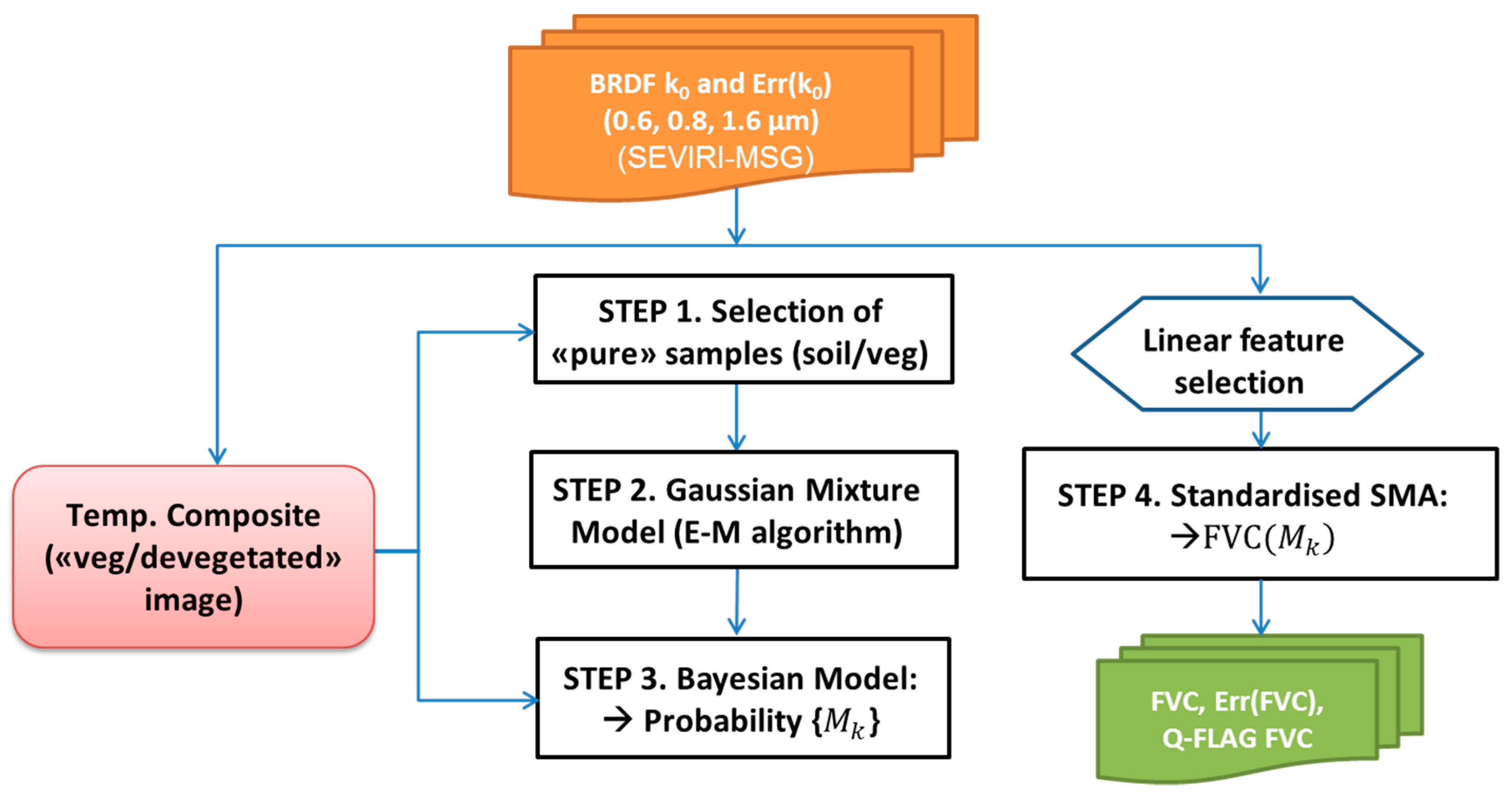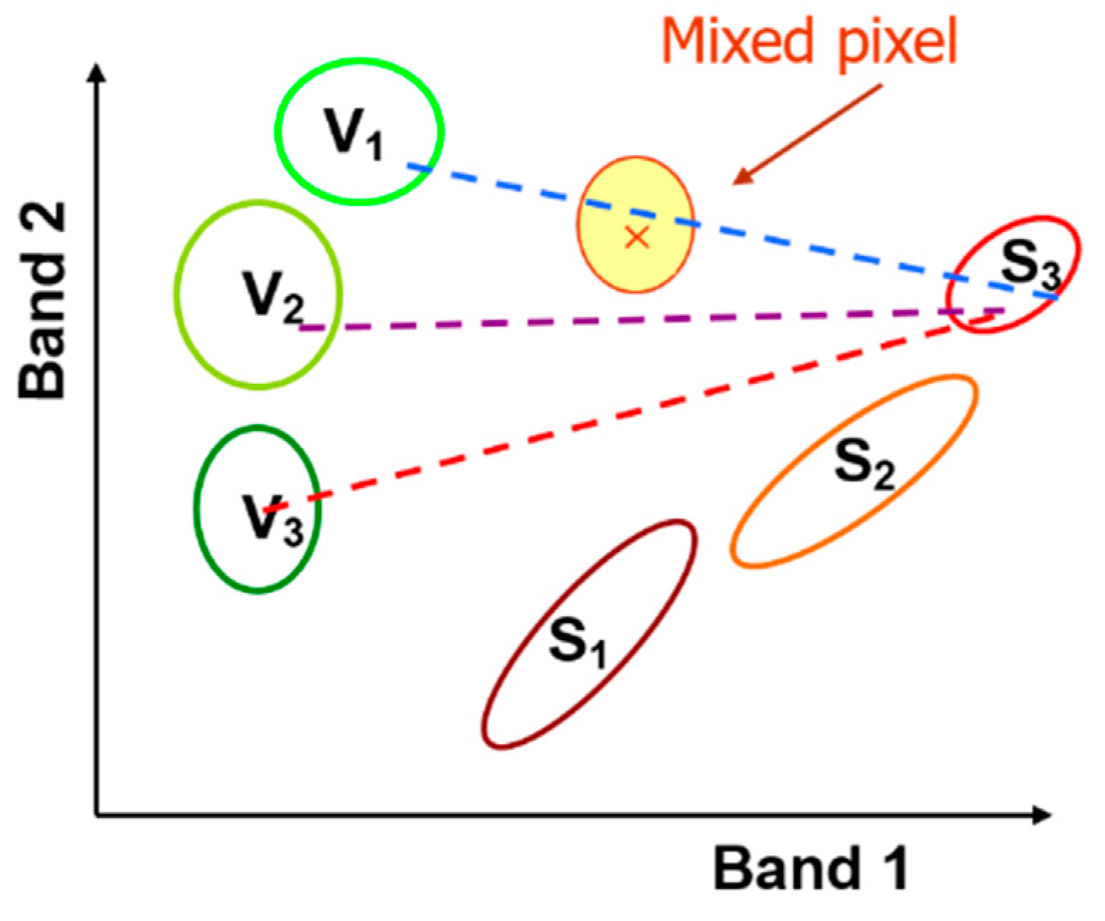An effective way to reduce this overestimation is underweighting the SWIR band (step 4 of the algorithm).

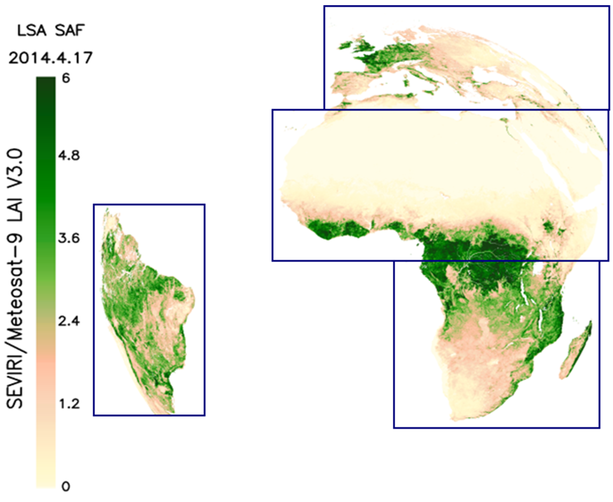
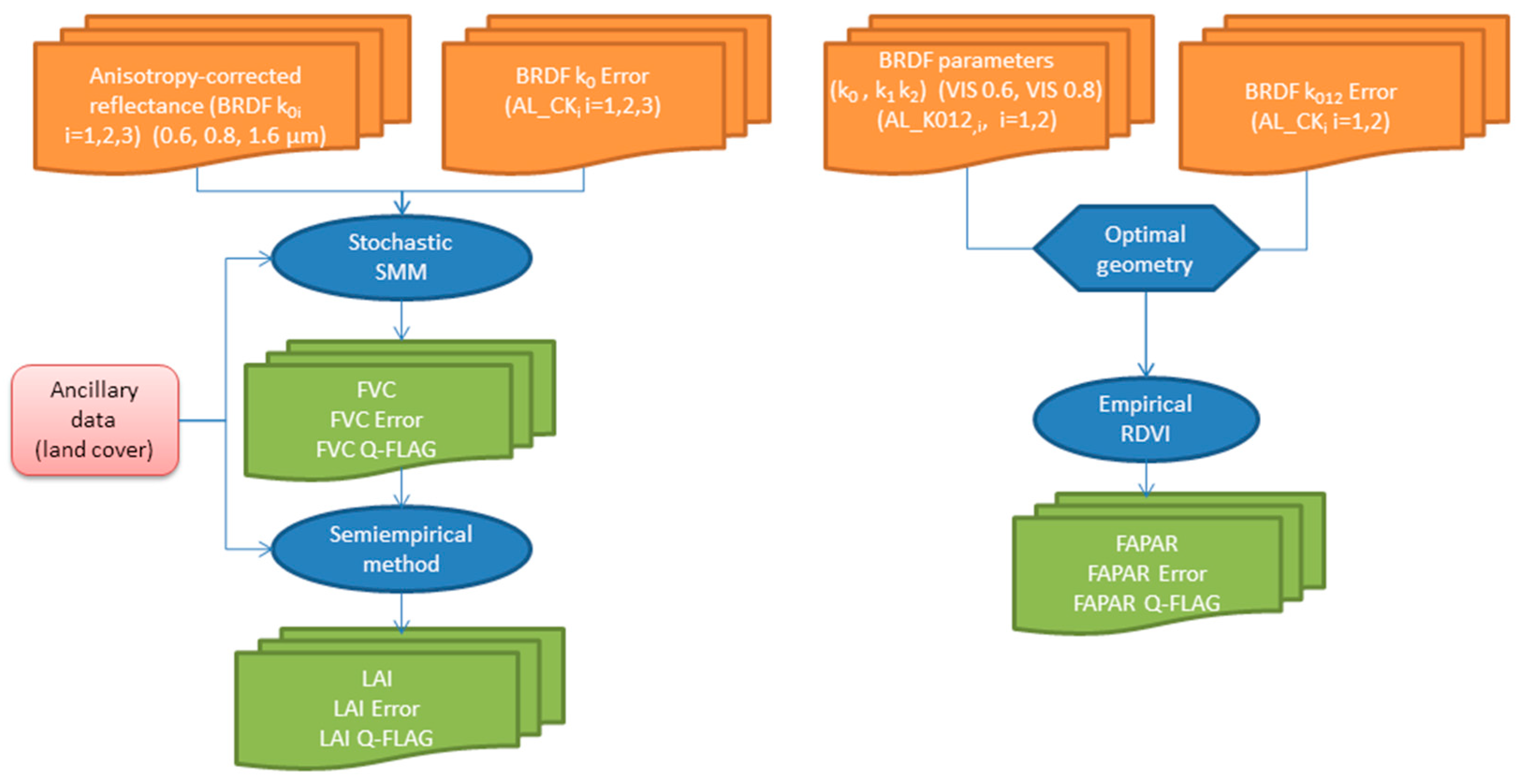
2.3. LAI Algorithm

The LSA SAF algorithm uses a pragmatic solution to the radiative transfer problem, which assumes a tractable physical model for interception of solar direct irradiance by leaf canopies [43]. By assuming that leaves are flat with bi-Lambertian properties, the total transmittance, which represents the fraction of incident radiation above the canopy which reaches the soil background level can be expressed as follows [47]:

$$T\left({\theta }_{\mathrm{s}}\right)=\exp [-b\left(G\left({\theta }_{\mathrm{s}}\right)/{\mu }_{\mathrm{s}}\right)\mathrm{LAI}],$$

(14)

where μ_s = cosθ_s, being θ_s the solar zenith angle, G(θ_s) is the average extinction function [48], $T\left({\theta }_{\mathrm{s}}\right)$ and b is the backscattered parameter, which can be roughly assumed to be equal to 0.945 for all vegetation types [49]. The fraction of solar radiation intercepted by the vegetation (FIPAR), which coincides with FVC when the sun and the observer are both at zenith, i.e., $\mathrm{FVC}=\mathrm{FIPAR}\left({\theta }_{\mathrm{s}}=0\right)$ is expressed as:

$$\mathrm{FIPAR}\left({\theta }_{\mathrm{s}}\right)=1-T\left({\theta }_{\mathrm{s}}\right)=1-\exp [-b\left(G\left({\theta }_{\mathrm{s}}\right)/{\mu }_{\mathrm{s}}\right)\mathrm{LAI}].$$

(15)

The above formulation assumes a random distribution of foliage elements, disregarding the increased probability of light penetration in clumped canopies. A clumping index Ω [50], which accounts for the degree of the deviation of foliage distribution from the random case, can be introduced in Equation (15) to correct possible underestimation of LAI [20]:

$$\mathrm{FVC}=\mathrm{FIPAR}\left({\theta }_{\mathrm{s}}=0\right)=1-\exp (-b\cdot G\left({\theta }_{\mathrm{s}}=0\right)\cdot \Omega \cdot \mathrm{LAI}).$$

(16)

It can be assumed for simplicity a value of 0.5 for the leaf projection factor G(θ_s) considering spherical orientation of the foliage. In order to avoid maximum LAI values in fully vegetated areas exceeding a value about 7, a coefficient a₀ in the range (1.04-1.07) is introduced in Equation (16):

$$\mathrm{FVC}=a_{\mathrm{o}}\{1-\exp (-0.5\cdot b\cdot \Omega \cdot \mathrm{LAI})\}.$$

(17)

A land cover-dependent clumping index is considered for each of the GLC2000 classes, which corresponds to the maximum values calculated from global POLDER multiangular data [51]. The values range from 0.68 for evergreen forest to 0.83-0.85 for herbaceous, shrub and cultivated areas (see Table S1 in Supplementary Material), leading to a conservative first-order correction of the clumping effect.

2.4. FAPAR Algorithm

The algorithm used for retrieving daily integrated green FAPAR is not novel but it relies on the method proposed by [32], a statistical relationship general enough for global applications based on simulations using the homogeneous SAIL (Scattering by Arbitrary Inclined Leaves) model [52]. The algorithm does not use any prior knowledge on the land cover. Although the SAIL model is widespread in the remote sensing community for the estimation of vegetation biophysical variables, limitations of homogeneous models should be more important in heterogeneous (e.g., savannas and open shrublands) or in canopies showing a complex architecture (e.g., boreal forest). More than 5000 soil/vegetation combinations varying leaf inclination distribution (LIFD), LAI, leaf transmittance, leaf reflectance and soil spectral albedo were considered. The diffuse fraction of incoming radiation was held constant and equal to 0.2, which represents clear sky conditions. For each scenario, red and NIR reflectances with variations of sun and view angles were derived from the SAIL model along with daily-integrated FAPAR, as computed by integration of the instantaneous FAPAR over the day:

$$\mathrm{FAPAR}=\frac{{{\displaystyle \int }}_t^{t^{\prime }}\mathrm{APAR}\mathrm{d}t}{{{\displaystyle \int }}_t^{t^{\prime }}\mathrm{PAR}\mathrm{d}t},$$

(18)

where t and t’ are the time for sunrise and sunset. The FAPAR was integrated over solar angles corresponding to a target located at 45°N latitude and at the equinox.

An optimal geometry based on the criteria of linearity and minimum dispersion between NDVI and daily-integrated FAPAR was found in the solar principal plane (θ_s=45°, θ_v=60°, ϕ=0°). The soil contribution to the canopy reflectance was reduced at this oblique view using a vegetation index, called RDVI (Renormalized Difference Vegetation Index), defined as follows:

$$\mathrm{RDVI}={\left(\mathrm{NDVI}·\mathrm{DVI}\right)}^{1/2}=\frac{\mathrm{NIR}-\mathrm{R}}{\sqrt{\mathrm{NIR}+\mathrm{R}}},$$

(19)

where DVI [16] is the difference vegetation index, defined as follows:

$$\mathrm{DVI}=\left(k_0\right)\mathrm{NIR}-\left(k_0\right)\mathrm{VIS}.$$

(20)

Finally, the RDVI-FAPAR relationship in the optimal geometry is given as follows:

$$\mathrm{FAPAR}=1.81 {\left(\mathrm{RDVI}\right)}_{\mathrm{opt}}-0.21,$$

(21)

where (RDVI)_opt refers to the RDVI computed in the optimal geometry. The reflectance in the optimal geometry for each spectral channel is estimated as follows [53]:

$$R_{\mathrm{opt}}\left(\lambda \right)=k_0\left(\lambda \right)-0.240k_1\left(\lambda \right)+0.202k_2\left(\lambda \right)$$

(22)

2.5. Products Uncertainty Estimation

A per-pixel estimate of the uncertainty for each prediction, namely ${\sigma }_{\mathrm{FVC}}$, ${\sigma }_{\mathrm{LAI}}$ and ${\sigma }_{\mathrm{FAPAR}}$, is provided, which propagates uncertainty of inputs and other variables involved in the calculations (see Equations in Supplementary Material).

3. The SEVIRI/MSG Vegetation Products

The LSA SAF generates and disseminates a suite of vegetation products derived from SEVIRI/MSG BRDF composited data for the whole Meteosat disk over land surfaces ideally free of snow and ice cover using the described algorithm at two different time resolutions (see Figure 6), daily (MDLAI, MDFVC, MDFAPAR), and 10-days (MTLAI, MTFVC, MTFAPAR) [54]. The characteristics of SEVIRI based products provided by the LSA SAF are described in

Table 1. Product Requirements for MSG vegetation products, in terms resolution and accuracy.

Product	Identifier	Distribution	Temporal Resolution	Spatial Resolution	Target Accuracy
MDFVC	LSA-421	NRT	1-day	MSG pixel	Max [0.075,15%]
MTFVC	LSA-422	NRT	10-days	MSG pixel	Max [0.075,15%]
MTFVC-R	LSA-450	CDR(1)	10-days	MSG pixel	Max [0.075,15%]
MDLAI	LSA-423	NRT	1-day	MSG pixel	Max [0.5,20%]
MTLAI	LSA-424	NRT	10-days	MSG pixel	Max [0.5,20%]
MTLAI-R	LSA-451	CDR(2)	10-days	MSG pixel	Max [0.5,20%]
MDFAPAR	LSA-425	NRT	1-day	MSG pixel	Max [0.075,15%]
MTFAPAR	LSA-426	NRT	10-days	MSG pixel	Max [0.075,15%]
MTFAPAR-R	LSA-452	CDR(3)	10-days	MSG pixel	Max [0.075,15%]

¹http://doi.org/10.15770/EUM_SAF_LSA_0003. ²http://doi.org/10.15770/EUM_SAF_LSA_0004. ³http://doi.org/10.15770/EUM_SAF_LSA_00035.

. Daily products use as input the MDAL BRDF parameters computed using a daily rolling compositing approach with a characteristic 5-day compositing period, whereas the 10-days product use as input the MTAL BRDF product based on a composite over a 30-day period. We refer for further details about the recursive temporal composition to Geiger et al. [33]. Using the latest version of the daily (v3.1) and 10-days (v1.2) algorithms, released in January 2016, the LSA SAF system generates and disseminated the products in Near-Real-Time (NRT) with a time lag of about six hours. NRT users are also encouraged to use EUMETCast (https://navigator.eumetsat.int), i.e., the primary distribution means for EUMETSAT image data and derived products.

The algorithms were reprocessed to generate the full archive of CDRs for 10-days vegetation products for FVC (MTFVC-R), LAI (MTLAI-R) and FAPAR (MTFAPAR-R) over the period 2004-2015, which complement the datasets available in the LSA SAF website since 2016 onwards. Both NRT products and homogeneous CDR 10-days vegetation products are available from the website (https://landsaf.ipma.pt/en/products/vegetation/). A similar dataset of reprocessed daily products has been produced as internal products for the period 2004-2015. Although the daily products are not foreseen to be distributed as CDR, they may be made available upon request.

The algorithm is firstly applied separately at four SEVIRI geographic regions: Europe (Euro), Northern Africa (NAfr), Southern Africa (SAfr), and South America (SAme) (see location in Figure 6). However, since the latest version (v3.1) onwards, products are disseminated for the whole Meteosat disk. The projection and spatial resolution correspond to the characteristics of Level 1.5 (standard geolocation) MSG/SEVIRI instrument data. Information on geo-location and data distribution is available at the LSA SAF web-site: http://landsaf.ipma.pt.

Each product is delivered in the Hierarchical Data Format version 5 (HDF5), which contains three separate datasets: a biophysical product, its respective error estimate and a Quality Flag (QF) field. The error dataset is a pixel-wise estimate of the observation uncertainty, which is indicative of the quality of the retrieval error (see details of calculation in Supplementary Material). These retrieval errors have shown to be within the range of the typical differences found between satellite products. For examples the uncertainty ranges typically between 0.05 and 0.10 for FVC, between 0.5 and 1.0 for LAI and between 0.05 and 0.20 for FAPAR. The FAPAR product presents a lower quality because it uses as input the three BRDF parameters (k₀, k₁, k₂), with k₂ presenting large uncertainties and noisy profiles on a short time scale, mainly in Western Africa.

The algorithms to retrieve LSA SAF vegetation require ideally free of snow and ice cover observations. Since snow events in previous days, though influencing the signal, may be unidentified BRDF product, an empirical criterion was used to identify and mask out pixels with residual, by combining the SEVIRI channels 1 (0.6 μm) and 3 (1.6 μm):

$$\begin{array}{c}{k}_0\left({\lambda }_1\right)-k_0\left({\lambda }_3\right)>0\\ or k_0\left({\lambda }_1\right)>k_{0,\max }\left({\lambda }_1\right)+0.06\\ or (k_0\left({\lambda }_1\right)>k_{0,\max }\left({\lambda }_1\right)+0.02 \mathrm{and} k_0\left({\lambda }_3\right)<k_{0,\min }\left({\lambda }_3\right))\end{array}$$

where $k_{0,\max }\left({\lambda }_1\right)$ and $k_{0,\min }\left({\lambda }_3\right)$ refer to the values of the $k_0$ devegetated image in channel 1 and 3, respectively. The QF records relevant information at the pixel level about the quality and processing status of retrievals (e.g., unrealistic input ranges, traces of inland water, traces of snow and retrieval values out of maximum physical range). The QF codes and several empirical thresholds used to blind problematic areas are shown in Tables S2 and S3 in Supplementary Material, respectively, as in the Product User Manual (available from http://landsaf.ipma.pt).

Figure 7 shows quality information of the SEVIRI/MSG FVC, LAI and FAPAR products, using the mean error of the products along the year 2014. Green color refers to consolidate regions with optimal quality. Reliable areas with medium quality are shown in cyan color. Orange color refers to regions with low quality. Finally, red color refers to generally unusable areas, presenting large view zenith angles and frequent snow cover (e.g., Europe during wintertime). FAPAR is generally unusable in areas with persistent cloud occurrence (e.g., western Africa).

The seasonal variations in the quality and coverage of the daily MSG FVC product along 2014 are depicted in Figure 8. Optimal or medium quality retrievals are obtained for north and south Africa continental zones with a negligible percentage of poor quality or missing values. An acceptable performance is also found over Europe from April through September, with a significant quality reduction during late autumn and winter. The worst performance is observed for south America regions, generally due to decreased accuracy and a larger percentage of missing values. Both daily MSG LAI and FAPAR products show similar performance stages with slightly lower rates of high quality values.

A detailed assessment of the MSG CDR products is provided in a validation report [55], showing good spatial and temporal consistency as compared to currently available validated vegetation products and no presence of artefacts. Noteworthy good inter-annual precision and stability of the long-term time series was found. Based on the validation results, performed over a representative network of sites over global conditions, CDR MSG vegetation products reached the operational status, what means that the products fulfilled all defined requirements and are suitable for distribution to users. Positive results were found for all the considered criteria, evaluated by comparisons with similar products such as Copernicus Global Land Monitoring Service GEOV1 based on SPOT/VGT data and NASA MODIS/TERRA products. Accuracy assessment against ground references provided by the Committee on Earth Observation Satellite (CEOS) through its Working Group in Calibration and Validation (WGCV) showed improved accuracy as compared to similar products and up to 84% of validation samples within target requirements [55].

Internal Consistency between the LSA SAF Products

Temporal profiles of the 10-days MSG vegetation products were verified through a comparison with the daily vegetation products. A very good agreement was found for the three products (see examples in Figure 9). Although one main drawback of the daily FAPAR product with regard to other operational products was the shaky temporal profiles on a daily basis, the 10-days (MTFAPAR) improves notably the smoothness of daily FAPAR.

The aim of this section is also to analyse the consistency among the suite of LSA SAF vegetation products (i.e., FAPAR and LAI) and albedo fields. The energy absorbed by the ground below vegetation (FGROUND) can be estimated by combining the FAPAR and an independent LSA SAF field from the albedo SEVIRI product, the bi-hemispherical reflectance integrated over the photosynthetically active spectral region (BHRPAR) [33]. From energy conservation, the fraction of PAR absorbed by the ground beneath the canopy is given by [56]:

$$\mathrm{FGROUND}=1-\mathrm{BHRPAR}-\mathrm{FAPAR},$$

(23)

Following previous works [56], FGROUND can be expressed as the downward PAR flux density, F, times the soil absorptance, 1−α, where α is the reflectance of the canopy background and F can be expressed via the Beer’s law [57]:

$$\mathrm{FGROUND}\approx \frac{1-\alpha }{1-\alpha {\mathrm{r}}^{*}}{\mathrm{e}}^{\left[-G\left({\theta }_{\mathrm{s}}\right)\mathrm{LAI}/\cos \left({\theta }_{\mathrm{s}}\right)\right]},$$

(24)

where r* is the probability that photon entering through the lower canopy boundary will be reflected back by the vegetated layer [58,59]. Figure 10 shows the relationship between MSG LAI and FGROUND for two SEVIRI regions, Europe (Euro), and southern Africa (SAfr), as derived from BHRPAR and FAPAR SEVIRI/MSG products using Equation (24). The distribution can be well approximated by the exponential function, $\mathrm{FGROUND}={\mathrm{Ae}}^{-\mathrm{B}·\mathrm{LAI}}$ for different periods, which indicates a strong consistency between LAI and FGROUND at the resolution of SEVIRI products.

4. Potential Applications of SEVIRI Vegetation Products

Different studies have assessed the quality of SEVIRI vegetation products [60,61,62]. MSG/SEVIRI LAI and FAPAR products were included in a detailed scientific analysis for quality information provision within the Evaluation and Quality Control (EQC) of climate data products derived from satellite and in situ observations to be catalogued within the Copernicus Climate Change Service (C3S) Climate Data Store (CDS) [63]. The products have been extensively used as input for environmental applications [64,65]. Particularly, the MSG LAI product found applicability to examine the feedback of land surface in response to vegetation changes [66], and in a hydrological model for flood early warning systems [67]. Gessner et al. [61] reported that the MSG LAI product is well suited to capture critical periods of growing cycle during the rainy season in West Africa as compared to existing global LAI products derived from polar orbit instruments. The use of MSG FVC and LAI products improved evapotranspiration estimates with respect to ECOCLIMAP-I in a land surface model [68]. Daily MSG LAI products were used for automatic derivation of detailed phenological information at the African continent [69]. The MSG LAI was fused with VGT/SPOT LAI to fill frequent gaps in VGT product during the rainy season in West Africa [70]. Further case studies and product applications of the SEVIRI/MSG vegetation products are provided in the LSA SAF web page (https://landsaf.ipma.pt/).

The SEVIRI/MSG vegetation products are routinely used as input in the operational line of several LSA SAF products. Daily MSG FVC and LAI are required inputs to update information about the state of vegetation for the derivation of the LSA SAF evapotranspiration and (latent and sensible) heat flux products [71]. The MSG FVC information on the pixel fraction of vegetation cover is required to operationally retrieve thermal Land Surface Emissivity [72]. The daily MSG FAPAR is also included as input on the Monteith’s LUE concept used for the computation of the 10-days Gross Primary Production (MGPP) product recently developed in LSA SAF [73,74]. The remaining of this section provides further insights about potential use of the LSA SAF vegetation products, considering three illustrative examples of land processes applications.

4.1. Application 1: Monitoring of Seasonal Cycle and Phenology

The enhanced data quality of geoestationary SEVIRI products can be demonstrated by comparing time series of FVC and polar-orbiting satellite sensors such as MODIS and SPOT/VGT across the cloud-prone equatorial regions, such as Amazonian, West Africa and Central Africa. As illustrated in a representative site in the western part of Equatorial Africa (Figure 11), the quality of polar-orbiting satellite products is severely hampered by cloud occurrence. The presence of missing values for long periods and unrealistic short-term variations reduces the ability of polar orbit products to capture the seasonal cycle.

Conversely, temporal profiles of MSG FVC are consistent from year to year showing realistic smooth variations, even during periods with high cloud coverage during the growing season. These findings are in line with previous studies [61,75]. This is mainly because the frequent sampling of its geostationary platform allows to accumulate enough cloud-free observations along a single day.

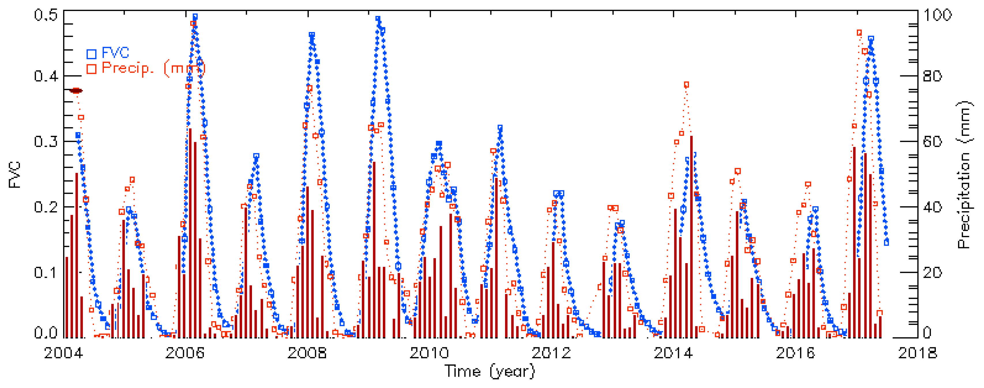
4.2. Application 2: Interrelation between Vegetation and Rainfall

Accumulated precipitation data derived from 10-days rainfall estimates (RFE 2.0) at a spatial resolution of 0.1° were considered to explore the performance of the SEVIRI FVC product over the Africa continent. The Rainfall Estimator (RFE) is produced by NOAA Climate Prediction Center (NOAA/CPC) merging information from polar-orbiting microwave measurements, geostationary infrared satellite estimates and gridded rainfall gauge measurements [76,77]. As illustrated in Figure 12, the SEVIRI FVC is an indicator of spatial and temporal rainfall variability, showing a strong temporal correlation with rainfall measurements (Pearson coefficient of determination r ranging from 0.7 to 0.9) in most of Africa.

Figure 13 shows an example of the relationships between FVC and 3-month accumulated rainfall for an herbaceous biome located in southern Africa. A clear interrelation is found between inter-annual variations of both magnitudes, proving the FVC product to be a proper indicator to detect sensitive areas. In particular, the rainfall deficit occurred during the rainy seasons of 2005, 2013, 2015 and 2016 produced a severe impact on the FVC during the growing season. Although not all regions present similar response to rainfall precipitation, NRT monitoring of FVC anomalies can be used to diagnose in below-normal rainfall values in sensitive areas, and inputted in early warning system of water stress initiation and severe drought events.

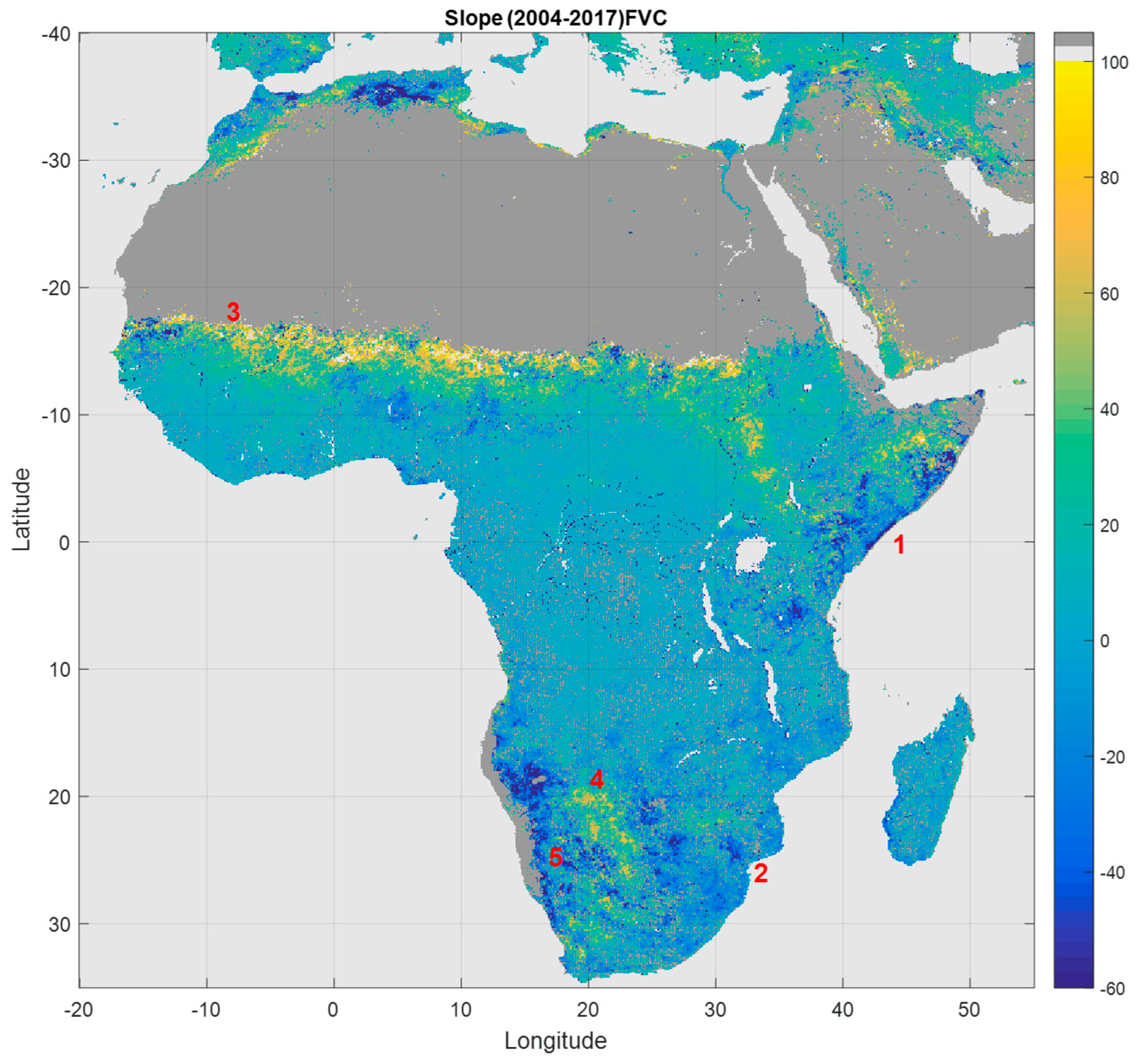
4.3. Application 3: The Detection of Inter-Annual Vegetation Trends over the Period 2004-2017

A trend analysis over Africa to report long-term variations due to subtle changes over the period 2004-2017 has been performed. A multiresolution analysis (MRA) wavelet transform (WT) has been applied to the 10-days MSG FVC product [78]. Figure 14 shows the derived normalized trend of inter-annual changes over Africa for the period 2004-2017. In general, no trend is observed over central Africa (light blue and green colors) with some distinguishable negative trend areas (dark blue colors) localized at eastern (Horn of Africa, region 1), southern Mozambique (region 2) and western Namibia (region 5). The impact on vegetation is particularly evident in these regions since they have been affected by a precipitation deficit due to El Niño-Southern Oscillation (ENSO) events [79,80,81]. Conversely, positive trend values (yellow colors) are mostly located in the grassland biomes of the Sahel zone (region 3) and a few patches in east of Namibia and west of Bostwana (region 4). The Sahel results agree with the widely reported re-greening behavior in this area for the last two decades [82,83] whereas the behavior of region 4 is possibly explained by exceptionally wet years in southwestern Africa since circa 2005.

5. Summary and Conclusions

This paper describes the algorithm currently used in the LSA SAF operational system to produce in NRT daily and 10-days basis global FVC, LAI and FAPAR biophysical products from SEVIRI/MSG data. A novel algorithm has been proposed to retrieve FVC, which is also the base for retrieving LAI using a semi-empirical method. It relies on a stochastic spectral mixture model which characterizes the large variability of soil background and target vegetation using statistical (Gaussian mixture) models with a finite number of classes, and determines a posteriori probabilities of the background/soil classes making use of the pixel multitemporal trajectory. The FAPAR algorithm uses statistical relationships with BRDF in an optimal angular geometry, general enough for global applications. This study evidences a good consistency among the suite of SEVIRI/MSG (daily and 10-days) vegetation products, as well as among FAPAR, LAI and BHRPAR, enabling a realistic partitioning of incoming solar radiation between the canopy and the ground below the canopy.

Main advantages and relevant information derived from this study are summarized below:

• NRT daily (MDFVC, MDLAI, MDFAPAR) and 10-days (MTFVC, MTLAI, MTFAPAR) products are generated and disseminated from LSA SAF since January 2004 over the geostationary Meteosat disk offering almost fifteen years of an alternative dataset to the user community.
• The 10-days (MTFVC-R, MTLAI-R and MTFAPAR-R) CDRs are provided as a suite of EUMETSAT climate products data records estimated consistently along the years using the latest versions of the whole processing chain algorithms. The 10-days products could be suitable for a community of users that requires observations representative of a 30-day period with at frequency of 10 days (e.g., numerical weather and climate models, and flood forecasting systems).
• The daily SEVIRI/MSG timeliness of the distribution of the observations and its smaller compositing period avoids possible shifts regarding the actual state of the vegetation (e.g., for an early estimate of key phenological parameters and seasonal production).
• The absence of gaps and the high temporal frequency and continuity of the products over Africa offer major potentials for NRT monitoring of land cover dynamics for applications that require frequent observations such as agriculture, and food management.
• The SEVIRI/MSG vegetation products have demonstrated its suitability to accurately resolving long term changes in large regions, allowing improving the understanding of interactions between land surface and climate.

The MSG programme is expected to provide observations for the next years to ensure long-term operations. In order to improve the coverage of the LSA SAF service, an ongoing work is the clone of MSG algorithms to produce similar LSA SAF products based on the Indian Ocean Data Coverage (IODC) observations. A priority work in LSA SAF is the adaptation of the algorithms to take advantage of enhanced capabilities in terms of spatial and spectral resolution of the future EUMETSAT sensors. The algorithm will be adapted to the enhanced characteristics of the Flexible Combined Imager (FCI)/Meteosat Third Generation satellites (MTG), allowing a more accurate characterization of the soil and vegetation signatures and improved screening of snow pixels. The FCI based products will ensure the continuity of the service during the lifetime of the MTG program.

References

- WMO. A Global Framework for Climate Services-Empowering the Most Vulnerable; WMO: Geneva, Switzerland, 2011. [Google Scholar]
- Hewitt, C.; Mason, S.; Walland, D. The Global Framework for Climate Services. Nat. Clim. Chang. 2012, 2, 831–832. [Google Scholar] [CrossRef]
- Dowell, M.; Lecomte, P.; Husband, R.; Schulz, J.; Mohr, T.; Tahara, Y.; Eckman, R.; Lindstrom, E.; Wooldridge, C.; Hilding, S.; et al. Strategy Towards an Architecture for Climate Monitoring from Space. 2013. Available online: http://www.wmo.int/pages/prog/sat/documents/ARCH_strategy-climate-architecture-space.pdf (accessed on 1 June 2019).
- Trigo, I.F.; Dacamara, C.C.; Viterbo, P.; Roujean, J.-L.; Olesen, F.; Barroso, C.; Camacho-de-Coca, F.; Carrer, D.; Freitas, S.C.; García-Haro, J.; et al. The Satellite Application Facility for Land Surface Analysis. Int. J. Remote Sens. 2011, 32, 2725–2744. [Google Scholar] [CrossRef]
- Schmetz, J.; Pili, P.; Tjemkes, S.; Just, D.; Kerkmann, J.; Rota, S.; Ratier, A. An introduction to Meteosat Second Generation (MSG). Bull. Am. Meteorol. Soc. 2002, 83, 977–992. [Google Scholar] [CrossRef]
- Liang, S. Comprehensive Remote Sensing; Elsevier: Amsterdam, The Netherlands, 2017. [Google Scholar]
- Chase, T.N.; Pielke, R.; Kittel, T.; Nemani, R.; Running, S. Sensitivity of a general circulation model to global changes in leaf area index. J. Geophys. Res. 1996, 101, 7393–7408. [Google Scholar] [CrossRef]
- Buermann, W.; Dong, J.; Zeng, X.; Myneni, R.B.; Dickinson, R.E. Evaluation of the utility of satellite-based leaf area index data for climate simulation. J. Clim. 2001, 14, 3536–3550. [Google Scholar] [CrossRef]
- Leuning, R.; Zhang, Y.Q.; Rajaud, A.; Cleugh, H.; Tu, K. A simple surface conductance model to estimate regional evaporation using MODIS leaf area index and the Penman–Monteith equation. Water Resour. Res. 2008, 44. [Google Scholar] [CrossRef]
- Pagani, V.; Guarneri, T.; Busetto, L.; Ranghetti, L.; Boschetti, L.; Movedi, E.; Campos-Taberner, M.; García-Haro, F.J.; Katsantonis, D.; Stavrakoudis, D.; et al. A high resolution, integrated system for rice yield forecast at district level. Agric. Syst. 2018, 168, 181–190. [Google Scholar] [CrossRef]
- Gilardelli, C.; Stella, T.; Confalonieri, R.; Ranghetti, L.; Campos-Taberner, M.; García-Haro, F.J.; Boschetti, M. Downscaling rice yield simulation at sub-field scale using remotely sensed LAI data. Eur. J. Agron. 2018, 103, 108–116. [Google Scholar] [CrossRef]
- López-Lozano, R.; Duveiller, G.; Seguini, L.; Meroni, M.; Garcia-Condado, S.; Hooker, J.; Leo, O. Towards regional grain yield forecasting with 1-km resolution EO biophysical products: Strengths and limitation at pan-European level. Agric. For. Meteorol. 2015, 206, 12–32. [Google Scholar] [CrossRef]
- Barlage, M.; Zeng, X. The effects of observed fractional vegetation cover on the land surface climatology of the community land model. J. Hydrometeorol. 2004, 5, 823–830. [Google Scholar] [CrossRef]
- Bojinski, S.; Verstraete, M.; Peterson, T.; Richter, C.; Simmons, A.; Zemp, M. The concept of essential climate variables in support of climate research, applications, and policy. Bull. Am. Meteorol. Soc. 2014, 95, 1431–1443. [Google Scholar] [CrossRef]
- CTOS. Implementation Plan for the Global Observing System for Climate in Support of the UNFCCC (2010 Update); GCOS Rep. 138; CTOS: Geneva, Switzerland, 2010; p. 186. Available online: https://library.wmo.int/doc_num.php?explnum_id=3851 (accessed on 9 September 2019).
- GCOS-200. The Global Observing System for Climate: Implementation Needs; Rep. 200; World Meteorological Organization; GCOS: Geneva, Switzerland, 2016; p. 315. Available online: https://library.wmo.int/doc_num.php?explnum_id=3417 (accessed on 9 September 2019).
- Roujean, J.-L.; Lacaze, R. Global mapping of vegetation parameters from POLDER multiangular measurements for studies of surface-atmosphere interactions: A pragmatic method and validation. J. Geophys. Res. 2002, 107, ACL6:1–ACL6:14. [Google Scholar] [CrossRef]
- Knyazikhin, Y.; Glassy, J.; Privette, J.L.; Tian, Y.; Lotsch, A.; Zhang, Y.; Wang, Y.; Morisette, J.T.; Votava, P.; Myneni, R.B.; et al. MODIS Leaf Area Index (LAI) and Fraction of Photosynthetically Active Radiation Absorbed by Vegetation (FPAR) Product (MOD15) Algorithm Theoretical Basis Document; NASA Goddard Space Flight Center: Greenbelt, MD, USA, 1999; Volume 20771. [Google Scholar]
- Hu, J.; Tan, B.; Shabanov, N.; Crean, K.A.; Martonchik, J.V.; Diner, D.J.; Knyazikhin, Y.; Myneni, R.B. Performance of the MISR LAI and FPAR algorithm: A case study in Africa. Remote Sens. Environ. 2003, 88, 324–340. [Google Scholar] [CrossRef]
- Gobron, N.; Pinty, B.; Verstraete, M.; Govaerts, Y. The MERIS Global Vegetation Index (MGVI): Description and preliminary application. Int. J. Remote Sens. 1999, 20, 1917–1927. [Google Scholar] [CrossRef]
- Bacour, C.; Baret, F.; Béal, D.; Weiss, M.; Pavageau, K. Neural network estimation of LAI, fAPAR, fCover and LAI×Cab, from top of canopy MERIS reflectance data: Principles and validation. Remote Sens. Environ. 2006, 105, 313–325. [Google Scholar] [CrossRef]
- Gobron, N.; Mélin, F.; Pinty, B.; Verstraete, M.M.; Widlowski, J.-L.; Bucini, G. A Global Vegetation Index for SeaWiFS: Design and Applications. In Remote Sensing and Climate Modeling: Synergies and Limitations SE-1; Beniston, M., Verstraete, M.M., Eds.; Springer: New York, NY, USA, 2001; Volume 7, pp. 5–21. [Google Scholar]
- Baret, F.; Hagolle, O.; Geiger, B.; Bicheron, P.; Miras, B.; Huc, M.; Berthelot, B.; Niño, F.; Weiss, M.; Samain, O.; et al. LAI, fAPAR and fCover CYCLOPES global products derived from VEGETATION: Part 1: Principles of the algorithm. Remote Sens. Environ. 2007, 110, 275–286. [Google Scholar] [CrossRef]
- Baret, F.; Weiss, M.; Lacaze, R.; Camacho, F.; Makhmara, H.; Pacholcyzk, P.; Smets, B. GEOV1: LAI and FAPAR essential climate variables and FCOVER global time series capitalizing over existing products. Part1: Principles of development and production. Remote Sens. Environ. 2013, 137, 299–309. [Google Scholar] [CrossRef]
- García-Haro, F.J.; Campos-Taberner, M.; Muñoz-Marí, J.; Laparra, V.; Camacho, F.; Sánchez-Zapero, J.; Camps-Valls, G. Derivation of global vegetation biophysical parameters from EUMETSAT Polar System. ISPRS J. Photogramm. Remote Sens. 2018, 139, 57–74. [Google Scholar] [CrossRef]
- Gitelson, A.A. Wide dynamic range vegetation index for remote quantification of biophysical characteristics of vegetation. J. Plant Physiol. 2004, 161, 165–173. [Google Scholar] [CrossRef] [PubMed]
- Widlowski, J.L.; Taberner, M.; Pinty, B.; Bruniquel-Pinel, V.; Disney, M.; Fernandes, R.; Gastellu-Etchegorry, J.P.; Gobron, N.; Kuusk, A.; Lavergne, T. Third Radiation Transfer Model Intercomparison (RAMI) exercise: Documenting progress in canopy reflectance models. J. Geophys. Res. Atmos. 2007, 112. [Google Scholar] [CrossRef]
- Weiss, M.; Baret, F.; Myneni, R.B.; Pragnere, A.; Knyazikhin, Y. Investigation of a model inversion technique to estimate canopy biophysical variables from spectral and directional reflectance data. Agronomie 2000, 20, 3–22. [Google Scholar] [CrossRef]
- Jacquemoud, S.; Verhoef, W.; Baret, F.; Bacour, C.; Zarco-Tejada, P.J.; Asner, G.P.; François, C.; Ustin, S.L. PROSPECT + SAIL models: A review of use for vegetation characterization. Remote Sens. Environ. 2009, 113, S56–S66. [Google Scholar] [CrossRef]
- Fisher, J.I.; Mustard, J.F.; Vadeboncoeur, M.A. Green leaf phenology at Landsat resolution: Scaling from the field to the satellite. Remote Sens. Environ. 2006, 100, 265–279. [Google Scholar] [CrossRef]
- Filipponi, F.; Valentini, E.; Nguyen Xuan, A.; Guerra, C.A.; Wolf, F.; Andrzejak, M.; Taramelli, A. Global MODIS Fraction of Green Vegetation Cover for Monitoring Abrupt and Gradual Vegetation Changes. Remote Sens. 2018, 10, 653. [Google Scholar] [CrossRef]
- Roujean, J.-L.; Breon, F.-M. Estimating PAR absorbed by vegetation from bidirectional reflectance measurements. Remote Sens. Environ. 1995, 51, 375–384. [Google Scholar] [CrossRef]
- Geiger, B.; Carrer, D.; Franchisteguy, L.; Roujean, J.L.; Meurey, C. Land surface albedo derived on a daily basis from Meteosat second generation observations. IEEE Trans. Geosci. Remote Sens. 2008, 46, 3841–3856. [Google Scholar] [CrossRef]
- Geiger, B.; Carrer, D.; Hautecoeur, O.; Franchistéguy, L.; Roujean, J.-L.; Catherine Meurey, X.C.; Jacob, G.; Algorithm Theoretical Basis Document (ATBD). Land Surface Albedo PRODUCTS: LSA-103 (ETAL). Available online: Ref: SAF/LAND/MF/ATBD_ETAL/1.3, 25 November 2016, 41 pp (accessed on 12 July 2019).
- Bartholome, E.; Belward, A.S. GLC2000: A new approach to global land cover mapping from earth observation data. Int. J. Remote Sens. 2005, 26, 1959–1977. [Google Scholar] [CrossRef]
- Bishop, C.M. Neural Networks for Pattern Recognition; Oxford University Press: Oxford, UK, 1995. [Google Scholar]
- McLachlan, G.J.; Krishnan, T. The EM Algorithm and Extensions; Wiley: New York, NY, USA, 1997. [Google Scholar]
- Stone, M. Comments on model selection criteria of Akaike and Schwartz. J. R. Stat. Soc. 1979, 41, 276–278. [Google Scholar]
- Fraley, C.; Raftery, A.E. Model-Based Clustering, Discriminant Analysis, and Density Estimation. J. Am. Stat. Assoc. 2002, 97, 611–631. [Google Scholar] [CrossRef]
- Garcia-Haro, F.J.; Sommer, S.; Kemper, T. A new tool for variable multiple endmember spectral mixture analysis (VMESMA). Int. J. Remote Sens. 2005, 26, 2135–2162. [Google Scholar] [CrossRef]
- Roberts, D.A.; Gardner, M.; Church, R.; Ustin, S.; Scheer, G.; Green, R.O. Mapping chaparral in the Santa Monica Mountains using multiple endmember spectral mixture models. Remote Sens. Environ. 1998, 65, 267–279. [Google Scholar] [CrossRef]
- Bateson, C.A.; Asner, G.P.; Wessman, C.A. Endmember Bundles: A New Approach to Incorporating Endmember Variability into Spectral Mixture Analysis. IEEE Trans. Geosci. Remote Sens. 2000, 38, 1083–1094. [Google Scholar] [CrossRef]
- Asner, G.P.; Heidebrecht, K.B. Spectral unmixing of vegetation, soil and dry carbon cover in arid regions: Comparing multispectral and hyperspectral observations. Int. J. Remote Sens. 2002, 23, 3939–3958. [Google Scholar] [CrossRef]
- Song, C. Spectral mixture analysis for subpixel vegetation fractions in the urban environment: How to incorporate endmember variability? Remote Sens. Environ. 2005, 95, 248–263. [Google Scholar] [CrossRef]
- Somers, B.; Asner, G.P.; Tits, L.; Coppin, P. Endmember variability in spectral mixture analysis: A review. Remote Sens. Environ. 2011, 115, 1603–1616. [Google Scholar] [CrossRef]
- Huete, A.R. A soil-adjusted vegetation index (SAVI). Remote Sens. Environ. 1988, 25, 295–309. [Google Scholar] [CrossRef]
- Roujean, J.-L. A tractable physical model of shortwave radiation interception by vegetative canopies. J. Geophys. Res. 1996, 101, 9523–9532. [Google Scholar] [CrossRef]
- Ross, J. The Radiation Regime and Architecture of Plant Stands; Springer Science & Business Media: Berlin, Germany, 2012; Volume 3. [Google Scholar]
- Roujean, J.-L.; Tanré, D.; Bréon, F.-M.; Deuzé, J.-L. Retrieval of land surface parameters from airborne polder bidirectional reflectance distribution function during hapex-sahel. J. Geophys. Res. Atmos. 1997, 102, 11201–11218. [Google Scholar] [CrossRef]
- Nilson, T. A theoretical analysis of the frequency of gaps in plant stands. J. Agric. Meteorol. 1971, 8, 25–38. [Google Scholar] [CrossRef]
- Chen, J.M.; Menges, C.H.; Leblanc, S.G. Global mapping of foliage clumping index using multi-angular satellite data. Remote Sens. Environ. 2005, 97, 447–457. [Google Scholar] [CrossRef]
- Verhoef, W. Light scattering by leaf layers with application to canopy reflectance modeling: The SAIL model. Remote Sens. Environ. 1984, 16, 125–141. [Google Scholar] [CrossRef]
- Roujean, J.-L.; Leroy, M.; Deschamps, P.-Y. A bidirectional reflectance model of the Earth’s surface for the correction of remote sensing data. J. Geophys. Res. Atmos. 1992, 97, 20455–20468. [Google Scholar] [CrossRef]
- Garcia-Haro, F.J.; Gilabert, M.A.; Melia, J. Linear spectral mixture modelling to estimate vegetation amount from optical spectral data. Int. J. Remote Sens. 1996, 17, 3373–3400. [Google Scholar] [CrossRef]
- Camacho, F.; García-Haro, F.J.; Fuster, B.; Sanchez-Zapero, J. MSG/SEVIRI Vegetation Parameters (VEGA) Validation Report. SAF/LAND/UV/VR_VEGA_MSG, v3.1. 2018, p. 109. Available online: https://landsaf.ipma.pt/en/products/vegetation/ (accessed on 9 September 2019).
- García-Haro, F.J.; Camacho-de Coca, F.; Meliá, J.; Martínez, B. Operational derivation of vegetation products in the framework of the LSA SAF project. In Proceedings of the 2005 EUMETSAT Meteorological Satellite Conference, Dubrovnik, Croatia, 19–23 September 2005. [Google Scholar]
- Diner, D.J.; Braswell, B.H.; Davies, R.; Gobron, N.; Hu, J.; Jin, Y.; Kahn, R.A.; Knyazikhin, Y.; Loeb, N.; Muller, J.-P.; et al. The value of multiangle measurements for retrieving structurally and radiatively consistent properties of clouds, aerosols, and surfaces. Remote Sens. Environ. 2005, 97, 495–518. [Google Scholar] [CrossRef]
- Hu, J.; Su, Y.; Tan, B.; Huang, D.; Yang, W.; Schull, M.; Bull, M.A.; Martonchik, J.V.; Diner, D.J.; Knyazikhin, Y.; et al. Analysis of the MISR LAI/FPAR product for spatial and temporal coverage, accuracy and consistency. Remote Sens. Environ. 2007, 107, 334–347. [Google Scholar] [CrossRef]
- Knyazikhin, Y.; Marshak, A. Mathematical aspects of BRDF modeling: Adjoint problem and Green’s function. Rem. Sens. Rev. 2000, 18, 263–280. [Google Scholar] [CrossRef]
- Wang, Y.; Buermann, W.; Stenberg, P.; Smolander, H.; Häme, T.; Tian, Y.; Hu, J.; Knyazikhin, Y.; Myneni, R.B. A new parameterization of canopy spectral response to incident solar radiation: Case study with hyperspectral data from pine dominant forest. Remote Sens. Environ. 2003, 85, 304–315. [Google Scholar] [CrossRef]
- Gessner, U.; Niklaus, M.; Kuenzer, C.; Dech, S. Intercomparison of leaf area index products for a gradient of sub-humid to arid environments in West Africa. Remote Sens. 2013, 5, 1235–1257. [Google Scholar] [CrossRef]
- Camacho, F.; García-Haro, F.J.; Sánchez-Zapero, J.; Fuster, B.; Validation Report MSG/SEVIRI Vegetation Parameters (VEGA). SAF/LAND/UV/VR_VEGA_MSG, Issue 3.1. 2017. Available online: http://www.landsaf.meteo.pt (accessed on 9 September 2019).
- Nightingale, J.; Mittaz, J.P.; Douglas, S.; Dee, D.; Ryder, J.; Taylor, M.; Old, C.; Dieval, C.; Fouron, C.; Duveau, G.; et al. Ten Priority Science Gaps in Assessing Climate Data Record Quality. Remote Sens. 2019, 11, 986. [Google Scholar] [CrossRef]
- Martínez, B.; Camacho, F.; Verger, A.; García-Haro, F.J.; Gilabert, M.A. Inter-comparison and quality assessment of MERIS, MODIS and SEVIRI fAPAR products over the Iberian Peninsula. Int. J. Appl. Earth Obs. Geoinf. 2013, 21, 463–476. [Google Scholar] [CrossRef]
- Verger, A.; Camacho, F.; García-Haro, F.J.; Meliá, J. Prototyping of Land-SAF leaf area index algorithm with VEGETATION and MODIS data over Europe. Remote Sens. Environ. 2009, 113, 2285–2297. [Google Scholar] [CrossRef]
- Mamadou, O.; Galle, S.; Cohard, J.M.; Peugeot, C.; Kounouhewa, B.; Biron, R.; Zannou, A.B. Dynamics of water vapor and energy exchanges above two contrasting Sudanian climate ecosystems in Northern Benin (West Africa). J. Geophys. Res.-Atmos. 2016, 121, 11–269. [Google Scholar] [CrossRef]
- Koriche, S.A.; Rientjes, T.H.M. Application of satellite products and hydrological modelling for flood early warning. Phys. Chem. Earth 2016, 93, 12–23. [Google Scholar] [CrossRef]
- Ghilain, N.; Arboleda, A.; Sepulcre-Canto, G.; Batelaan, O.; Ardo, J.; Gellens-Meulenberghs, F. Improving evapotranspiration in a land surface model using biophysical variables derived from MSG/SEVIRI satellite. Hydrol. Earth Syst. Sci. 2012, 16, 2567–2583. [Google Scholar] [CrossRef]
- Guan, K.; Medvigy, D.; Wood, E.F.; Caylor, K.K.; Li, S.; Jeong, S.J. Deriving vegetation phenological time and trajectory information over Africa using SEVIRI daily LAI. IEEE Trans. Geosci. Remote Sens. 2014, 52, 1113–1130. [Google Scholar] [CrossRef]
- Klein, C.; Bliefernicht, J.; Heinzeller, D.; Gessner, U.; Klein, I.; Kunstmann, H. Feedback of observed interannual vegetation change: A regional climate model analysis for the West African monsoon. Clim. Dyn. 2017, 48, 2837–2858. [Google Scholar] [CrossRef]
- Arboleda, A.; Ghilain, N.; Meulenberghs, F. First Product User Manual for MET&DMET (v2) and new LE&H products. Available online: SAF/LAND/RMI/PUM/ET&SF/1.1, 2018, 35 pp (accessed on 12 July 2019).
- Trigo, I.F.; Peres, L.F.; DaCamara, C.C.; Freitas, S.C. Thermal land surface emissivity retrieved from SEVIRI/METEOSAT. IEEE Trans. Geosci. Remote Sens. 2008, 46, 307–315. [Google Scholar] [CrossRef]
- Martínez, B.; Sánchez-Ruiz, S.; Gilabert, M.A.; Moreno, A.; Campos-Taberner, M.; García-Haro, F.J. Retrieval of daily gross primary production over Europe and Africa from an ensemble of SEVIRI/MSG products. Int. J. Appl. Earth Obs. 2018, 65, 124–136. [Google Scholar] [CrossRef]
- Martínez, B.; Gilabert, M.A.; Sánchez-Ruiz, S.; Campos-Taberner, M.; García-Haro, F.J.; Brüemmer, C.; Carrara, A.; Feig, G.; Grünwald, T.; Mammarella, I.; et al. Evaluation of the LSA-SAF Gross Primary Production product derived from SEVIRI/MSG data (MGPP). ISPRS J. Photogramm. Remote Sens. 2019. in review. [Google Scholar]
- García-Haro, F.J.; Camacho, F.; Verger, A.; Meliá, J. Current status and potential applications of the LSA-SAF suite of vegetation products. In Proceedings of the 29th EARSeL Symposium, Chania, Greece, 15–18 June 2009. [Google Scholar]
- Xie, P. CPC RFE Version 2.0. NOAA/CPC Training Guide; Drought Monitoring Centre: Nairobi, Kenya, 2001. [Google Scholar]
- Laws, K.B.; Janowiak, J.E.; Huffman, G.J. Verification of rainfall estimates over Africa using RFE, NASA MPA-RT, and CMORPH. In Proceedings of the Combined Preprints CD-ROM, 84th AMS Annual Meeting, Paper P2.2 in 18th Conference on Hydrology, Seattle, WA, USA, 11–15 January 2004; p. 6. [Google Scholar]
- Martínez, B.; Gilabert, M.A. Vegetation dynamics from NDVI time series analysis using the wavelet transform. Remote Sens. Environ. 2009, 113, 1823–1842. [Google Scholar] [CrossRef]
- Loewenberg, S. Humanitarian response inadequate in Horn of Africa crisis. Lancet 2011, 378, 555–558. [Google Scholar] [CrossRef]
- Archer, E.R.M.; Landman, W.A.; Tadross, M.A.; Malherbe, J.; Weepener, H.; Maluleke, P.; Marumbwa, F.M. Understanding the evolution of the 2014–2016 summer rainfall seasons in southern Africa: Key lessons. Clim. Risk Manag. 2017, 16, 22–28. [Google Scholar] [CrossRef]
- Qu, C.; Hao, X.; Qu, J.J. Monitoring Extreme Agricultural Drought over the Horn of Africa (HOA) Using Remote Sensing Measurements. Remote Sens. 2019, 11, 902. [Google Scholar] [CrossRef]
- Brandt, M.; Mbow, C.; Diouf, A.A.; Verger, A.; Samimi, C.; Fensholt, R. Ground and satellite-based evidence of the biophysical mechanisms behind the greening Sahel. Glob. Chang. Biol. 2015, 21, 1610–1620. [Google Scholar] [CrossRef] [PubMed]
- Nicholson, S.E.; Funk, C.; Fink, A.H. Rainfall over the African continent from the 19th through the 21st century. Glob. Planet. Chang. 2017, 165, 114–127. [Google Scholar] [CrossRef]