Abstract
Understanding extraterrestrial environments and landforms through remote sensing and terrestrial analogy has gained momentum in recent years due to advances in remote sensing platforms, sensors, and computing efficiency. The seasonal brines of the largest salt plateau on Earth in Salar de Uyuni (Bolivian Altiplano) have been inadequately studied for their localized hydrodynamics and the regolith volume transport across the freshwater-brine mixing zones. These brines have recently been projected as a new analogue site for the proposed Martian brines, such as recurring slope lineae (RSL) and slope streaks. The Martian brines have been postulated to be the result of ongoing deliquescence-based salt-hydrology processes on contemporary Mars, similar to the studied Salar de Uyuni brines. As part of a field-site campaign during the cold and dry season in the latter half of August 2017, we deployed an unmanned aerial vehicle (UAV) at two sites of the Salar de Uyuni to perform detailed terrain mapping and geomorphometry. We generated high-resolution (2 cm/pixel) photogrammetric digital elevation models (DEMs) for observing and quantifying short-term terrain changes within the brines and their surroundings. The achieved co-registration for the temporal DEMs was considerably high, from which precise inferences regarding the terrain dynamics were derived. The observed average rate of bottom surface elevation change for brines was ~1.02 mm/day, with localized signs of erosion and deposition. Additionally, we observed short-term changes in the adjacent geomorphology and salt cracks. We conclude that the transferred regolith volume via such brines can be extremely low, well within the resolution limits of the remote sensors that are currently orbiting Mars, thereby making it difficult to resolve the topographic relief and terrain perturbations that are produced by such flows on Mars. Thus, the absence of observable erosion and deposition features within or around most of the proposed Martian RSL and slope streaks cannot be used to dismiss the possibility of fluidized flow within these features.
1. Introduction
Unmanned aerial vehicles (UAVs) or drones have revolutionized the possibilities of remote imaging and terrain modeling due to several advantages over the conventional spaceborne and aerial platforms [1,2]. Spaceborne platforms suffer from various limitations, such as fixed revisit times, cloud- and weather-related noise (except for microwave imaging), and extremely high costs for sub-meter resolution data. Similarly, conventional airborne platforms, such as helicopters and aircrafts, cannot fly in bad weather or below low-level clouds and have extremely high operational costs for image acquisition on a repeating basis. UAVs are remotely piloted reusable motorized aerial vehicles that are lightweight and easily transportable to remote places and can carry various types of payloads and cameras that are designed for specific purposes [1]. Thus, UAVs are adaptable to various research needs in terms of providing flexibility with timings of data acquisition, revisits, data/sensor types (multispectral, photogrammetric stereos, thermal/night imaging, hyperspectral, microwave, and light detection and ranging (LiDAR)), flying altitudes, viewing angles, and overlap dimensions. UAVs have the potential to act as a bridging platform between spatially discontinuous field observations and spatially continuous but costlier and coarser spaceborne remote sensing. Most importantly, the acquisition and operational costs of such automated systems are considerably lower, thereby providing better imaging options to a wide variety of user groups. For these reasons, in recent years a multitude of UAV-based studies have emerged in nearly all natural science domains, such as agriculture e.g., [3,4,5], forestry e.g., [6,7,8,9,10], urban mapping e.g., [11], geomorphology e.g., [12], glaciology e.g., [1], submerged vegetation mapping e.g., [13,14]; physical geography e.g., [15], mine monitoring e.g., [16,17], landscape dynamics e.g., [18], archaeology e.g., [19], bathymetry e.g., [20], and coastal dynamics e.g., [21,22]. An unprecedented growth in computational efficiency in recent years has resulted in several software and hardware packages that are capable of handling vast amounts of UAV data and enabling the processing and generation of precise high-resolution structure-from-motion (SfM)-based digital elevation models (DEMs) and orthomosaics of any terrain [23]. Interested readers can obtain more information on the features of various commercial UAVs, their hardware components and specifications, and their interdisciplinary applications from several key research papers and review articles e.g., [1,2,24,25,26,27]. Here, our objective is to derive high-resolution geomorphometric information about a briny salt flat environment in cold arid conditions that are similar to those on Mars using UAV data.
Salt flats are one of the most dynamic, mineral-rich, and heterogeneous landforms [28], often displaying strong fluvio-aeolian interactions [29]. In fact, such fluvio-aeolian interactions in drylands, such as Salar de Uyuni, have important environmental and ecological implications and deserve focused research at various spatiotemporal scales [30]. Vast salt flats account for nearly half of the world’s lithium reserves [31] and also provide significant quantities of boron and potash [32]. The high economic importance of salt flats, in addition to the high ecological and tourist value of their associated peripheral brines and saline water lagoons, explains the recent global interest in salt flat hydrogeology [32]. Salt flats are of two broad types: Coastal and continental. The main focus of remote sensing-based monitoring of saline environments on earth has been on the coastal environs to observe land degradation e.g., [33], vegetation mapping of tidal flats and salt marshes e.g., [34,35], environmental changes e.g., [36], species identification and mapping e.g., [37], land use/land cover changes e.g., [38], topography and geomorphology e.g., [39], and land deformations e.g., [40]. Nevertheless, the sequential study of continental salt flats is equally relevant for several research areas. Playas or dry salt lakes, as zones of groundwater discharge, act as important sources of water in cold arid regions, such as South American salt flats, where playa groundwater and brines support the mining industry and local flora and fauna [41]. Information about hydrology and groundwater table changes in continental salt flats are of substantial importance in monitoring local aquifer changes e.g., [42] and salt losses from the crust e.g., [43]. Such salt flats are also rich in various minerals and their mapping and monitoring can facilitate precise mineralogical estimation e.g., [44]. In addition, natural weathering rates of salty rocks can provide a clue about the landscape evolution of a region e.g., [45]. Continuous monitoring of continental salt flats is also important in evaluating the effectiveness of salt-replenishment projects for conserving the local ecosystem e.g., [46]. Monitoring of continental salt flats further facilitates paleo-environmental and paleo-climatic interpretation in desert and evaporitic sediments [29]. Moreover, since a major water input to such continental salt flat systems is lateral inflow with minor contributions from direct rainfall (due to the atmospheric aridity) and the only output is evaporation [32], the surficial and hydrological changes in salt flat systems can be used as a proxy in studying the effects of climate change [47]. Terrestrial salt crack polygons and salt flat environments can function as Martian analogues e.g., [48] to understand Martian desiccation cracks e.g., [49] and extraterrestrial life e.g., [50]. In fact, aeolian processes acting on fluvial deposits are known to aid in the formation of polygonal patterns and dunes [29]. Thus, a comprehensive and high-resolution understanding of the geomorphological features and seasonal dynamics of brine-rich salt flats not only helps us understand their responses to climatic and anthropogenic factors and characterize all aspects of the water budget, especially the elusive evaporation component, but also improves our knowledge of analogous extraterrestrial landforms, such as Martian desiccation cracks and probable brines.
Wetlands are commonly present in the margins of salt flats as a result of discharge of groundwater at the resulting freshwater-brine mixing, which is characterized by a mixing zone or saline interface [32]. Ecologically, these wetlands are some of the most sensitive regions and the monitoring of the salt flat mixing zones is of importance for managing mineral resources and associated ecosystems. In this regard, after a careful literature survey, we identify several research gaps to the best of our knowledge. First, there is no study on UAV-based high-resolution 3D and geomorphometric mapping of a continental salt flat environment. A recent study [32] has established how crucial such 3D information can be in modeling the hydrodynamics and the freshwater-brine mixing zones in salt flats. Second, there is no published research that elaborates on the short-term intra-seasonal terrain changes of the briny salt flat environment. Third, these salt flat brines were recently established as analogues for probable briny features on Mars [51,52] and a high-resolution investigation, such as the present work, was needed to monitor their flow characteristics. Here, our aim is not to participate in the debate on whether or not such liquid brines can exist on contemporary Mars. The premise of our research is based on the fact that several studies propose surface features such as recurring slope lineae (RSL) e.g., [53,54] and slope streaks e.g., [55,56,57] as plausible Martian brines with transient liquid water activity. RSL form a significant constituent of Martian “special regions” [58,59,60]. Moreover, there are contradictory views on whether RSL are watery flows [54,61,62,63,64,65], dry processes [66], or a combination of both [67,68]. Even if they are water related features, we have different opinions on the probable amount of liquid water flowing within them [67,69,70,71].
In order to prove or to disprove such hypotheses we must perform more rigorous analogue studies. Establishing and using a terrestrial brine environment as a Martian analogue site for such possibly briny surface features can be an important step in this direction. Identifying such research prospects of using UAVs for Mars research, the National Aeronautics and Space Administration (NASA) is sending the first UAV to Mars with the agency’s Mars 2020 rover mission, which is currently scheduled to launch in July 2020 [72]. We discuss this aspect of the Mars analogy in detail in the subsequent sections. Thus, the present research aims at filling the research gaps with the following objectives:
- To perform UAV-based high-resolution repeat survey and 3D data generation for the mixing zone of a continental salt flat environment;
- To generate geomorphometric parameters for the mixing zone of a continental salt flat environment;
- To observe short-term geomorphometric changes in the brines and their surroundings;
- To quantify the rate of regolith volume transport within such natural brines and to discuss their possible analogies with the proposed Martian brines.
In the following sections, we briefly introduce the study area and why it can be called a Mars brine analogue environment. We also provide details on the methods of high-resolution 3D data generation and morphometric analyses that we used in this study. We further discuss the implications of our temporal analyses for understanding the rheology of the possible Martian brines.
2. Study Area and Brine Seasonality
The identified Martian brine analogue environment is in Salar de Uyuni in Bolivian Altiplano (Figure 1). Salar de Uyuni is the largest salt flat on Earth, with an area of ~10,000 km2 [73]. This salt flat is situated at an elevation of 3653 m above sea level [74]. In this region within the southern hemisphere, the coldest and driest months are from May to September with zero rainy days on average, a mean relative humidity (RH) of ~35%, and an average minimum temperature of −7.5 °C [75] (Figure 2). The flatness of the terrain in this vast salt flat and the homogeneous reflectance allow for in-orbit satellite calibration of multispectral sensors, radiometers, and altimeters [75].
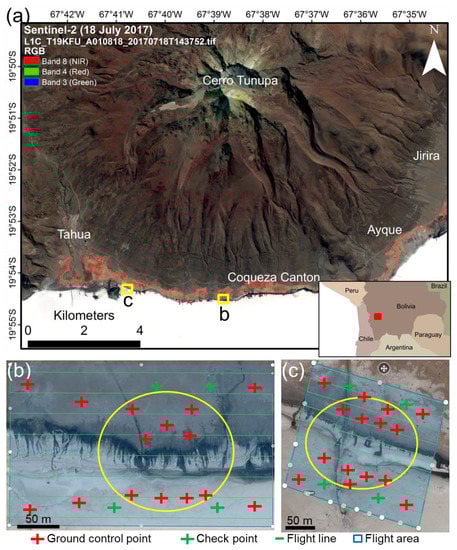
Figure 1.
Location map and flight lines. (a) A contextual map of the study sites in false color composite (RGB:843). The red rectangle in the inset political map in (a) shows the geographical location of the study sites. The yellow rectangles show the relative positions of the two flight sites, (b) Location 1 and (c) Location 2. The yellow circles in (b) and (c) highlight our areas of interest in the middle, which are surrounded by the maximum number of ground control points. Image credit for (a): Produced from European Space Agency (ESA) Sentinel-2 remote sensing data acquired under the European Commission’s Copernicus Program and downloaded from United States Geological Survey (USGS) EarthExplorer. Image credit for (b) and (c): Produced using DroneDeploy flight planning freeware with a Google Earth (GE) image collected on 15 September 2013 in the background, and the data provider for the GE image is National Centre for Space Studies (CNES)/Airbus.
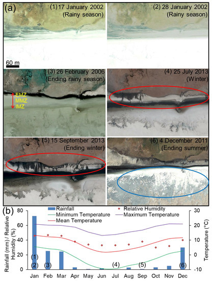
Figure 2.
Brine seasonality on the slopes. (a) Available high-resolution images from different seasons. The red ellipses highlight the emergence and growth of brines throughout the winter. The blue ellipse signifies the freshly precipitated salt evaporites. The double-headed red arrow shows various regions of the mixing zone (IMZ: Internal mixing zone, MMZ: Middle mixing zone, and EMZ: External mixing zone). (b) Meteorology of the study area. The plotted meteorological data have been derived from Table 1 of Lamparelli et al. [75]. The numbers on the bar plots represent the corresponding images in (a). The data provider for the GE images in (a) is CNES/Airbus.
The mapped areas cover the lowest slopes of Cerro Tunupa, a dormant volcano, where these slopes meet the salt flat (Figure 1). Figure 2 compiles all the available high-resolution satellite images for a section of these slopes and displays the significantly changing terrain within the seasons of a hydrological year. In January–February, the region experiences its highest precipitation in the form of rainfall (Figure 2b) and the terrain is washed-off, with a bright homogeneous salt flat that is distinctively visible (the upper panel of Figure 2a). By the end of February (the middle panel of Figure 2a), when the groundwater levels are at maximum and very close to the surface due to the recent rainfall events, the freshwater-brine interface lies at the external mixing zone (EMZ) at higher elevations. In July, when the temperatures are the lowest, there is absolutely no rainfall and the RH remains sufficient for promoting deliquescence and brine formation (Figure 2b), we start observing new dark streaks that originate at EMZ on the Tunupa slopes, which continue to grow through the winter until September–October (within the red ellipses in Figure 2a). By December, the temperature reaches its highest value and active evaporation leads to fading and disappearance of the shallow brines, which leave behind freshly precipitated salts (the blue ellipse in Figure 2a). During these months, we also observe the shifting of the freshwater-brine interface to the internal mixing zone (IMZ) at lower elevations.
The idea behind the present work was to study the Salar de Uyuni brines as analogues for the proposed Martian brines. RSL on Mars are seasonal, like Salar de Uyuni brines, but are relatively smaller understandably because of extremely low possible water volumes in the RSL. Another kind of proposed brines on Mars called slope streaks are not seasonal but are just a one-time phenomenon and are of the order of same magnitudes as Salar de Uyuni brines. Thus, in slope streak there are only one time terrain changes which occur and since we do not see any remarkable changes in the best Martian images of ~25 cm/pixel resolutions for a wide majority of slope streaks, it again tells us that the terrain changes are very minute possibly due to low volume of liquid water and need better spatial resolutions to get resolved. Thus, the prime requisites for an earth analogue to study these proposed Martian brines is that it has to be seasonal (like RSL) and it has to be studied while the water volumes in it are still lower (like both, RSL and slope streaks) during the formation season. In fact, the water volume that should be present in RSL throughout the season will still be lower than the volume, which the Salar de Uyuni brines could generate just in several days due to the relatively higher RH and more favorable temperatures. As one can see in Figure 2a, just in one and a half months of brine season (July–September) these small developing Salar de Uyuni brines turn into huge pools. The days when we opted for field work were carefully selected when the brines were not too small to observe small temporal scale changes and not too huge to make them irrelevant as an analogue. Thus, making more dynamical observations, which could last over several weeks was not ideal in the present case and whichever observations we had to take, it had to be within a short-temporal span since a couple of days of water activity in Salar de Uyuni is almost equivalent to the expected seasonal water activity in RSL on Mars. The study area was identified using high-resolution temporal Google Earth (GE) images, which showed significant brine seasonality (Figure 2) on the slopes. We planned the field work during 22–26 August 2017 for two locations that are ~4 km apart (Figure 1). The month of August was selected because the brines were not overly developed to completely cover the slopes and not too underdeveloped to show insignificant variations at the diurnal scale. Moreover, the briny water was transparent during the days on which field work was conducted and the base terrain was clearly visible, thereby allowing for drone-based geomorphometry and terrain modeling. The subsequent methodological steps are discussed in the following sections. Although the mixing zone predominantly displayed south-facing slope-orientation (aspect) with similar brine morphologies, we tried to select two mapping locations (Figure 1b,c) based on several dissimilarities. The two locations showed slight differences in slope and aspect conditions, with Location 2 (Figure 1c) being slightly steeper and facing south-west direction, in contrast to the south-facing gentler slopes at Location 1 (Figure 1b). Location 1 had interconnected and larger brines (maximum length ~65 m on 22 August 2017) compared to Location 2, where several of the brines were separated and comparatively smaller, with the largest brine reaching up to a length of ~52 m on 22 August 2017. Due to the slightly steeper slopes, the observed brine changes at Location 2 were more prominent on diurnal scales than at Location 1. Hence, we decided to perform the repeat flight for Location 2 at a two-day interval (22 August and 24 August) and for Location 1 at a four-day interval (22 August and 26 August) to better capture the short-term changes.
3. Materials and Methods
The following methodological steps were taken to achieve the research objectives.
3.1. Ground Control Points (GCPs)
The main objective of the field trip was to perform repeated UAV flights at two different locations and generate temporal DEMs and orthomosaics. These repeat DEMs that were generated for different days were used to measure elevation and other geomorphometric changes. Thus, we needed ground control points (GCPs) as common reference points or tie points (TPs) for enforcing a common georectification during the process of generating temporal DEMs. This enforced proper co-registration of the DEMs and made them mutually comparable to obtain accurate differencing results and geomorphometric changes. Therefore, more than ensuring the absolute positional accuracy of the GCP coordinates, which would have ideally required the use of a differential global positioning system (DGPS) unit, our objective was to use the GCPs as TPs to ensure relative positional accuracy and the same coordinates for the repeat DEMs for further comparison. The generic term for such GCPs is “stereo ground control points (SGCPs)” as an SGCP is a cross between a regular GCP and a TP. SGCPs have known ground coordinates (latitude, longitude, and elevation) with acceptable accuracy and are clearly identifiable in two or more images; however, the pixels and line locations vary for each image. Therefore, in addition to determining the relationship between the raw images and the ground, like a GCP, an SGCP also identifies how the images relate to each other, like a TP. The use of SGCPs further results into a stronger mathematical model for terrain modeling. Thus, although extreme absolute accuracy in GCPs was not mandatory for our study, we opted for one of the best possible handheld global positioning system (GPS) options for quick and acceptable GCP collection, which is suitable for our research objectives. We used a Garmin eTrex® 30x, which is one of the most accurate handheld GPS units that are presently available and has been widely utilized in various kinds of environmental research in recent years [76,77,78,79]. This GPS has significantly improved accuracy over other hand-held devices due to its ability to use both global navigation satellite system (GLONASS) and GPS satellites. In addition, as shown in Figure 1 and Figure 2, the field locations were widely open areas without any vegetation, habitation, and cliffs; thus, the reception of the navigation satellites was extremely good and they provided stable and reliable GPS readings. The Garmin eTrex® 30x GPS unit also provides the option of increasing the accuracy of GCPs via a feature, namely, “waypoint averaging”, by collecting multiple samples over a duration, which the unit automatically averages out to provide the most accurate final coordinates.
For both locations, we started collecting GCPs in the morning of 22 August using two Garmin eTrex® 30x GPS units; in total, 19 GCPs were collected for each of the locations in the stable areas (Figure 1b,c), 15 of which were used as SGCPs while four were used as check points to estimate the positional inaccuracies in the generated DEMs. The markers that were used to clearly identify the GCPs in the UAV images were similar to those that are depicted in Figure 1b,c (the red plus marks on white-background cardboard paper of dimensions 30 cm × 30 cm), with the middle of each plus mark used as a GPS recording point. We also made use of the waypoint averaging feature of the GPS unit by recording four points for each location with a 5-minute time interval between each reading. We inserted thin sticks in the middle of the markers after taking all the readings for each point to facilitate their location for placing the markers again, prior to the repeat flights. However, before the next flights, we further confirmed the locations of the markers by comparing them with 22 August GPS readings. All the GCPs were well-distributed, with highest densities in the middle of the flight rectangles, surrounding our points of interest (the yellow circles in Figure 1b,c).
3.2. UAV and Flight Planning
The UAV that was used for the present study was the DJI Phantom 4 Pro quadcopter (Figure 3a,b). This UAV has a weight (including the battery and propellers) of 1.388 kg, a diagonal size (excluding the propellers) of 35 cm, and a maximum flight time of ~30 minutes. The drone has a maximum service ceiling of ~6000 m above sea level (asl); in the present work, we flew it below ~3730 m asl. The UAV is resistant to a maximum wind speed of 10 m/s with an operating temperature range of 0 °C–40 °C and is equipped with an integrated 3-axis gimbal that provides an extremely narrow angular vibration range (±0.02°) and always maintains the preferred camera look-angle. We flew in calm wind conditions with clear skies (Figure 3) between the local times of ~10 am and 2 pm on all the days when the brines were not frozen, starting at Location 1 and proceeding to Location 2. DJI Phantom 4 Pro uses both GPS and GLONASS satellites and operating frequencies of 2.4–2.483 GHz and 5.725–5.825 GHz, which provide it a high hover accuracy range with respect to GPS positioning (vertical: ±0.5 m; horizontal: ±1.5 m) up to 7 km from the launch site.
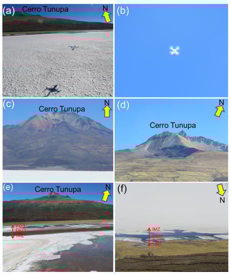
Figure 3.
Several of the field photographs that were captured between 22 and 26 August 2017. (a) The unmanned aerial vehicle (UAV) during lift-up. (b) The UAV at the top altitude of 60 m from the surface. (c,d) are pictures of Cerro Tunupa from Location 1 and Location 2, respectively. The double-headed red arrows in (e,f) show various regions of the mixing zone (IMZ: Internal mixing zone, MMZ: Middle mixing zone, and EMZ: External mixing zone). Field photograph credit: Group of Atmospheric Science, Luleå University of Technology.
The DJI Phantom 4 Pro camera uses a 1″ complementary metal-oxide semiconductor (CMOS) sensor that produces photographs with standard RGB channels. The 20-megapixel sensor has a manually adjustable aperture from F2.8 to F11; it supports autofocus with a focus range from 1 m to infinity and a field of view (FOV) of 84° and has a mechanical shutter for still imaging while the UAV is moving fast or the object of interest is dynamic. This camera sensor provided us a high spatial resolution of 1.8 cm/pixel, even from a flying altitude of 60 m. The selection of the flying altitude represents a trade-off between the pixel resolution, the completion of the entire flight with only one battery, and a substantial number of photographs (~300 for each location) to enable faster post-processing. Table 1 highlights the various flight plan and image parameters that we employed in the DroneDeploy flight planning freeware during the field data acquisition. The launch and landing sites were the same for all the flights at each location. To increase the density and accuracy of the point clouds and stereo-imaging, we ensured a high degree of overlap (side overlap = 70% and front overlap = 85%) between the images.

Table 1.
Flight plan and image parameters.
3.3. Generation of DEMs and Orthomosaics
The aerial photos were processed for DEM and orthomosaic generation using Agisoft PhotoScan Pro stand-alone licensed software. Agisoft PhotoScan Pro is a stand-alone software package that performs photogrammetric processing of digital images and generates 3D spatial data that are compatible with other GIS applications using structure-from-motion (SfM) photogrammetry, which was originally developed by Ullman [80]. For UAV-based surface modeling, Agisoft PhotoScan Pro is a proven performer amongst several widely used software packages, such as Erdas-LPS, EyeDEA (University of Parma), Pix4UAV, and PhotoModeler Scanner [81]. Agisoft PhotoScan has been widely used in a variety of environmental research in recent years e.g., [16,82,83,84].
Agisoft PhotoScan Pro has a fully automated workflow for 3D reconstruction and, in addition to its proven capability for accurate surface modeling e.g., [81], PhotoScan has several other advantages that suited our project and objectives: It comes at an affordable cost; it has a user-friendly graphic interface, and can derive sensor parameters intrinsically to perform calibration, local processing, and high-resolution and robust 3D modeling to generate outputs in multiple file formats that are compatible with other geospatial software [82]. A detailed account of the inherent SfM procedure and the workflow in PhotoScan are presented in Verhoeven [85]. Here, we briefly discuss the steps for deriving DEMs and orthomosaics from the aerial survey data. Agisoft PhotoScan Pro can generate the DEM in three primary stages:
1. Photograph alignment (bundle adjustment): Agisoft PhotoScan aligns the series of photos from a UAV survey using the camera location coordinates and algorithms to automatically detect stable common features among the images and determine the location and alignment of each camera position with respect to others [81,82]. This process is also called bundle adjustment and it generates a 3D sparse point cloud using the stereo-imaging, projection, and intersection of pixel rays from the different positions [82]. Depending on the computational efficiency of the processing computer, these steps can take widely varying times to complete and the selection of the processing parameters typically involves a trade-off between the computation time, the required accuracy, and the resolution of the results. However, for the entire data processing task, we employed a highly efficient computer with the following specifications: (i) Central processing unit (CPU): Intel Xeon E5-2650 v4, 12 cores, 24 threads, (ii) random-access memory (RAM): 256 GB, and (iii) graphics card: Nvidia Geforce Titan XP 12 GB GDDR5X. This computer enabled us not to compromise on any processing parameter, and we opted for the highest values for running the algorithms. For photograph alignment, we opted for the “Highest” accuracy and the highest possible numbers of tie points and key points in the processing tool window. For both locations, the photograph alignment took several hours and the results of the alignment process are shown in Figure 4.
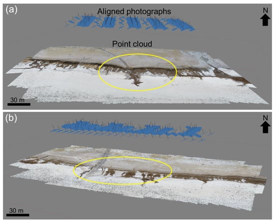
Figure 4.
Aligned photographs and dense point clouds for (a) Location 1 and (b) Location 2 for 22 August 2017 surveys that were generated in the Agisoft PhotoScan Pro stand-alone licensed software. The yellow ellipses highlight our areas of interest in the middle, densest portion of the point clouds.
2. Geometry building and dense point cloud generation: Before beginning this step, we can import GPS-derived GCPs into the processing and use the GCP markers that are observable in the images to assign more accurate GCP locations to the computed dense point cloud instead of proceeding with the on-board UAV GPS-based locations. The GCP coordinates also enable us to create a local coordinate system for precise scaling and alignment of the point cloud. A densification technique is applied on the already-generated sparse point cloud to derive a 3D dense point cloud using multi-view stereopsis (MVS) or depth mapping techniques [86]. The field GCP markers were observed, reviewed, and corrected in ~35% of the photographs that were captured for both locations. After this manual transfer of the local coordinates of the GCPs to the photographs, the model geometry is corrected via the Optimize Alignment tool in PhotoScan, followed by the intrinsic process of matching features to complete the final phase of geometry building to generate an accurate high-resolution 3D dense point cloud [82]. For this step, we opted for the “Ultra high” processing parameter and “Aggressive” depth filtering to derive the best possible results; the formed dense point cloud is shown in Figure 4. Our areas of interests were the middle, densest portions of the point clouds (the yellow ellipses in Figure 4) that were surrounded by the maximum number of GCPs (the yellow ellipses in Figure 1b,c).
3. Texture building and DEM generation: In this step, the generated 3D dense point cloud provides a continuous surface that can be triangulated and rendered with the original imagery to build a textured 3D mesh and create the final digital surface model [82] and, subsequently, the orthomosaics. For the DEMs, the dense point cloud was selected as the source data, with enabled interpolation and a pixel resolution of 2 cm/pixel, and WGS 1984 UTM Zone 19S as the coordinate system. For orthomosaics generation, the DEMs were selected as surface data, with enabled hole filling and 2 cm/pixel output resolution.
3.4. Geomorphometry
We focused on deriving first- and second-order terrain derivatives, such as the slope, aspect, curvature, and surface roughness, for geomorphometric analyses e.g., [55,87,88,89,90,91]. We employed the Spatial Analyst toolbox of the ArcGIS software version 10.6.1 to derive the slope, aspect, and curvature geomorphometric parameters. For a given elevation pixel, the Slope tool computes the maximum rate of change in the elevation value from that pixel to its eight adjoining pixels, whereas the Aspect tool determines the alignment of the slope in terms of the maximum rate of change from each pixel to its eight neighbors [88,92]. The Curvature tool of the Spatial Analyst toolbox calculates the second-order derivative of the input surface on a per-pixel basis for each pixel, for which a fourth-order polynomial is fitted to a surface that is composed of a 3 × 3 window [88,93,94]. We used the Geospatial Data Abstraction Library (GDAL) Roughness tool within the QGIS 2.18.23 software to derive surface roughness. The Roughness tool accepts elevation data as input and calculates the largest inter-cell difference of a central pixel and its surrounding pixels for each pixel [95]. We used the Reclassify tool within the Spatial Analyst toolbox of ArcGIS 10.6.1 to further classify the aspect, curvature, and roughness geomorphometric parameters into various classes, as shown in Figure 5 and Figure 6. The aspect and curvature classification schemes are explained in the respective tool help sections of the ArcGIS 10.6.1 software. To classify the surface roughness parameter, we employed the “Natural Breaks” option as this classification is based on natural groupings that are inherent to the data and classes are identified based on similar values and maximum differences between classes [96]. In order to obtain the error limit for our difference DEMs, we used the equation (1) as proposed by Etzelmüller [97].
where, Mean ∆h is the mean error in elevation difference, and Mean h1 and Mean h2 are the mean elevation errors in the repeat DEMs.
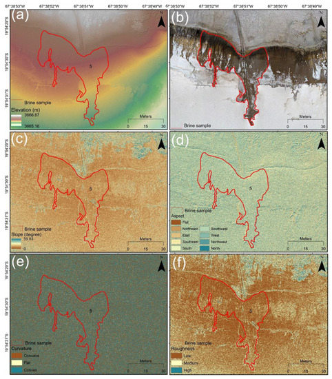
Figure 5.
Terrain at Location 1. (a) Digital elevation model (DEM), (b) orthomosaic, (c) slope, (d) aspect, (e) curvature, and (f) roughness. The numbers and red polygons indicate the brine samples that we selected for further analyses.
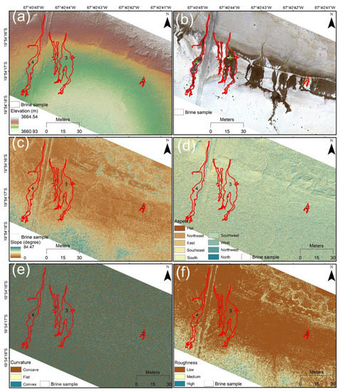
Figure 6.
Terrain at Location 2. (a) DEM, (b) orthomosaic, (c) slope, (d) aspect, (e) curvature, and (f) roughness. The numbers and red polygons indicate the brine samples that we selected for further analyses.
4. Results and Discussions
The following sections summarize the key results of our study within the predefined objectives.
4.1. DEMs, Orthomosaics, and Geomorphometric Parameters
The DEMs, orthomosaics, and other geomorphometric parameters are shown in Figure 5 and Figure 6 for Locations 1 and 2, respectively. The briny water was transparent during all the days on which field work was conducted and the base terrain was clearly visible (Figure 5b and Figure 6b), thereby allowing for drone-based imaging, geomorphometry, and terrain modeling. We selected five morphologically distinct brine samples for the analyses from the two locations as the representatives of all the brine streams in the region. The morphological characteristics of these samples are listed in Table 2. As discussed previously, several smaller and disjoint brines (Samples 1–4) were observed at Location 2 and we started the analyses from there. Location 1 had the largest sample (Sample 5), which was a composite of multiple contributing brines that were attached to one another. The longest brine sample was Sample 4, while Sample 5 had the largest areal span. Sample 2 was the smallest and represented a newly developed brine stream. Samples 1 and 4 displayed a largely linear morphology, which was most similar to RSL and the majority of the slope streaks that have been observed on Mars [55,98]. However, Martian slope streaks are also known to display a wide range of morphologies, such as fan-shape, curvilinear, and splitting/branching [51] (Figure 7). A striking morphological similarity is observed between Samples 1 and 4, and the curvilinear slope streaks (Figure 7e). The slope streaks are large-scale features on Mars with the usual dimensions about an order of magnitude larger than the Salar streaks (Figure 7e).
Table 2.
Selected morphologically distinct brine samples. All the given dimensions are based on observations that were made on 22 August 2017.
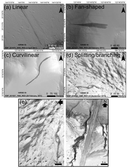
Figure 7.
Several of the most common morphologies of Martian slope streaks. (a) Linear, (b) fan-shaped, (c) curvilinear, (d) splitting/branching, and (e) Martian slope streaks (left) and Samples 1 and 4 (right) from Salar de Uyuni (in grayscale for comparison). High Resolution Imaging Science Experiment (HiRISE) image credit: NASA/JPL/University of Arizona.
In Table 3, we have summarized the characteristics of the geomorphometric parameters that were derived from the 22 August 2017 DEM for all the brine samples that are shown in Figure 5 and Figure 6. As mentioned above, we used check points for comparing the generated DEMs with GPS measurements and average absolute difference between DEMs and GPS coordinates were found to be 2.3 mm in horizontal and 2.8 mm in vertical. It should be noted that the GPS unit used by us can have inherent geolocation inaccuracy of 1–2 m on flat surfaces and the discussed results henceforth should be considered accordingly in terms of their absolute accuracy. Despite differing in size, Samples 1 and 4 showed similar elevation ranges, with the same mean elevation of ~3661.96 m. However, being the longest of all the brines, Sample 4 displayed remarkably higher values for local slopes (mean = 6.66°), curvature (mean = −0.21 mm−1), and roughness (mean = 6.69 mm) due to its stretch throughout all the mixing zones. In addition, the significantly higher standard deviation values for all these parameters for Sample 4 further demonstrate the wide terrain variability within this brine. All the brines displayed, on average, a more concave (negative mean value) curvature owing to slow subsurface erosion by the flowing brines. Another point worth mentioning here is that these five brines exhibited widely variable slope ranges at their initiation points. The slopes at the points of initiation varied from as high as ~40° for Sample 1 to as low as ~3° for Sample 4. Such broad slope ranges have also been displayed by the triggering points of Martian slope streaks, with ~8% of streaks originating even at gentler slopes of <10°, which are unsuitable for any dry-mass movement flow e.g., [55].
Table 3.
Characteristics of the geomorphometric parameters that were derived from the 22 August 2017 DEM.
4.2. Short-Term Geomorphometric Changes in the Brines and their Surroundings
To estimate the changes in the geomorphometric parameters between 22 and 26 August at Location 1 and 22 and 24 August at Location 2, we subtracted the geomorphometric rasters of 26 August and 24 August from the corresponding 22 August rasters. In Table 4, we have compiled the statistics regarding the observed changes and several interesting inferences can be made based on them. The average rates of bottom surface elevation change for brines were ~0.6 mm/day at Location 1 and ~1.44 mm/day at Location 2. According to the elevation changes, the least developed and smallest sample, namely, Sample 2, understandably displays minimal volumetric mass movement and elevation change from 22 to 24 August at Location 2 (Table 4). While we understand that all the average absolute differences between DEMs and GPS coordinates as reported in Section 4.1 are in the mm-range and their quantification can further be improved by more repeat surveys and DGPS-based field measurements, the nearly one-tenth (~0.1) of a pixel co-registration accuracy provides us an acceptable control over the reported elevation changes in the DEMs (Table 4). Such surficial changes are clearly observable in Figure 8 and Figure 9, thus removing any doubt from the selection of the pixel resolution that we opted for this research. Moreover, our DEM differencing results are in the mm-scale and still larger than one-tenth of the 2 cm/pixel DEM resolution (Table 4) as compared to several other well-cited studies e.g., [97,99,100], which report mean elevation differences, which are even lesser than one-tenth of the pixel resolutions of their respective DEMs. Here, we are going to compare two models for each of the locations and consistent with respect to each other, but due to the lack of precise DGPS inputs, may also likely be deformed at the start. This means that even individual DEM derivatives derived from these DEMs can have some level of uncertainty. However, by using same methods, processing parameters, and SGCPs, we have ensured that the level of these intrinsic deformations (if any) is similar, coherent, and consistent between the repeat DEMs as our main aim here is to observe the “changes” between the repeat DEMs. When we compared the elevations of subsequent DEMs (22 and 26 August at Location 1 and 22 and 24 August at Location 2) at all 30 stable GCPs and eight check points for both locations (Figure 1b,c), we observed an extremely low average deviation of 2.8 ± 0.3 mm, which can be attributed to our use of the same flight plans, GCPs, and image processing system and parameters for DEM and orthomosaic generations. The average of mean error in the difference DEMs at eight check points for both the locations as calculated using equation 1 was found to be ~3.9 mm. However, in terms of absolute accuracy, again this error is in addition to the intrinsic GPS errors as mentioned above.
Table 4.
Geomorphometric changes (mean ± standard deviation) in and around brine samples that were derived from the consecutive UAV acquisitions. Please note that the average of mean error in the difference DEMs at eight checkpoints was found to be ~3.9 mm for both the locations.
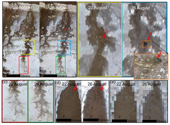
Figure 8.
Surficial changes in the brines. (a) Sample 2, with areas showing signs of minimal (red and green rectangles) and maximal (yellow and blue rectangles) mass transport. (b) The red arrow highlights the area from where significant regolith removal occurred between 22 and 24 August and the orange rectangle highlights the same area in a field photograph (credit: Group of Atmospheric Science, Luleå University of Technology) that was captured on 24 August. (c) The terminus of the brine where no visible topographic change could be observed, except the brine-stained surface. (d) Significant mass transport and regolith removal (red arrow) in an adjacent, larger brine. (e) Resampled versions of the brine that is shown in (d) with decreased resolution from 2 cm/pixel to 30 cm/pixel.
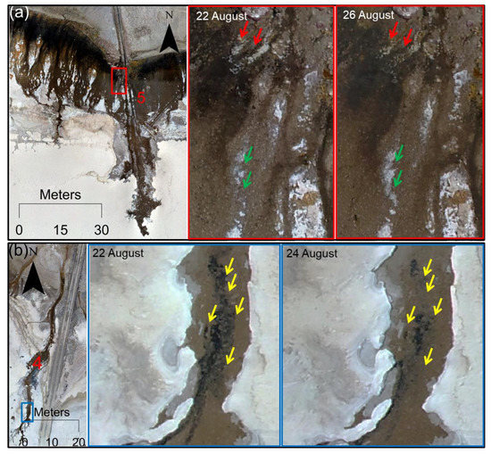
Figure 9.
Erosion, surface deposition, and pit deposition in brine samples. (a) Red arrows indicate signs of salt erosion and green arrows indicate surface deposition in subsequent images of Sample 5. (b) Yellow arrows indicate numerous troughs near the terminus of Sample 4 on 22 August, which were substantially filled by 24 August.
The bottom surface elevation changes during the consecutive mapping days; thus, the corresponding volumetric mass movement values essentially agree with the brine size and areal coverage for Location 2 (Table 2 and Table 4). However, despite being significantly larger than the brine samples at Location 2 (Table 2), Sample 5 at Location 1 showed elevation changes that were greater than those of only the smallest brine (Sample 2). Additionally, we must take into account that Sample 5 was revisited after four days, in contrast to the two-day observation gap for the samples at Location 2. However, Sample 5 still showed considerably lesser surficial changes, which further demonstrates the significant role that terrain parameters, such as the slope and aspect, could play in defining the flow and mass movements within such brines. The mean slope for Sample 5 was smaller compared to other samples (Table 3) and the slope can be a decisive parameter in controlling the flow rates and mass movement.
Several other inferences can be made from the statistics that are listed in Table 4. For example, the standard deviations of the bottom surface elevation changes for the brines at both locations are of the same order of magnitude as the corresponding elevation changes, thereby indicating significant variability. This high variability in elevation changes can be explained by localized salt and regolith removal at specific areas within the brines (Figure 8b,d). In Figure 8a, we highlight a region within Sample 2 (yellow and blue rectangles) that displayed significant elevation changes within the two days between the consecutive flights. The orange rectangle and the inset image in Figure 8b show a zoomed-in view and a field photograph of this area, respectively. Since Sample 2 was the smallest and least developed brine sample that we selected and within two days we observed regolith removal, we also examined an adjacent brine that was larger and relatively well-developed and found considerable evidence (Figure 8d) that at short temporal scales, such localized regolith removals can take place within these terrestrial brines. All the brines except Sample 4 displayed increases in surface slope and roughness, with significantly higher corresponding standard deviation values (Table 4). However, for Sample 4, the slope and roughness decreased during the days of observation and the standard deviation values were nearly twice those of the other samples. Sample 4 was narrow and the longest sample, with ~4 m of elevation change from the point of its initiation to its terminus (Table 2), and had nearly double the slope and roughness values of the other samples (Table 3); hence, it could not only have a faster erosion rate but also be unsuitable for supporting intra-brine depositions of displaced regolith in regions that have nearly flat slopes, thereby decreasing the surface roughness within the brine in general. Such downslope depositions of removed regolith over the plane surface within the brines have been observed in the other samples (Figure 9a) with gentler slopes. However, towards the terminus of Sample 4, we observed an area that was full of troughs on 22 August but was substantially filled with the sedimentation of eroded salt and regolith on 24 August (Figure 9b), which further explains the observed decrease in the surface roughness. Thus, such longer brines that traverse across all the mixing zones contribute significantly towards long-range salt, regolith, and nutrient mixing and mass transfer in continental salt flats.
On average, for all the brine samples, the local curvature in general and the concavity of the surface in particular increased during the observation periods (Table 4). Being a second-order derivative of the input surface, such an increase in the curvature at certain places is a direct indicator of erosion and surface depressions that are generated on short temporal scales of 2–4 days. This increase in local curvature was prominent for Samples 4 and 5 (Table 4) and, as shown in Figure 9, these were the brines that exhibited maximal terrain changes in terms of erosion and deposition, which is possibly due to the narrower and faster flows in Sample 4 and the steeper terrain and significant volume of the developed brine in Sample 5, which could dissolve and displace substantial amounts of salt and regolith. In addition, we performed an analysis to identify changes in the immediate vicinity of the brine samples. Considering the rate of brine-induced perturbations, we demarcated a 3 m buffer area around all the brine samples in the 22 August orthomosaics for monitoring the terrain changes within this buffer and observed slight increases in the surface elevations (Table 4) due to the deposition of transferred salts and regolith by the brines. On average, the increases in terrain elevation were 0.08 mm/day for Sample 5 at Location 1 and 0.21 mm/day for the brine samples at Location 2 (Table 4). The observed standard deviations in the changed elevation values were nearly double the values, which demonstrated that substantial parts of these buffer areas not only gained deposited salt and regolith but also lost salt and regolith due to the expansion in the brines during the observation periods. In addition, the altitudinal disparities between the removed salts and regolith from the brines and the deposited salts and regolith around the brines (Table 4) demonstrate the importance of intra-brine regolith shifts at diurnal scales.
4.3. Salar de Uyuni as an Analogue for the Martian Brine Environment
Several terrestrial analogues for expected Martian brines have been reported. They exhibit a seasonality that is similar to that of RSL and a morphology that is similar to slope streaks as reported from the McMurdo Dry Valleys, Antarctica e.g., [55,56,62,101,102,103]. Understandably, the terrestrial meteorology is too dynamic to allow the formation and sustained existence of natural brines in open environments as finding regions with coexisting salty dust and favorable atmospheric deliquescence conditions is extremely difficult on Earth and even if a briny feature is formed, there is always the possibility that high temperatures, a precipitation event, or dust storms could erase or obliterate it. If we consider the plausible briny origin of Martian RSL or slope streaks, then precise studies of the short-lived terrestrial brines are necessary for making inferences regarding the possible formation, geochemistry, and rheology of the proposed Martian brines. To achieve these objectives, we must first identify and characterize the limited number of such analogue sites that exist on Earth.
As one of the pioneering works in this regard, Head et al. [56] reported slope streak analogues from the Upper Wright Valley in Antarctica. The formation mechanism of these analogues, as proposed by Head et al. [56], involves melting of seasonal snowpack, followed by percolation and downslope migration of the meltwater into the dry substrate over the impermeable permafrost layer. In the finer-grained colluvium at lower elevations, capillarity draws this meltwater towards the surface, thereby wetting it and forming the streaks. Thus, the mechanism that was proposed by Head et al. [56] was not entirely related to salt-based deliquescence. In later years, Levy et al. [103] reported more such analogues from the adjacent Taylor Valley in Antarctica and called them “water tracks”. Although they also suggested that the features were a result of snow and ice melts, as proposed by Head et al. [56], Levy et al. [103] further established that these water tracks dynamically conveyed the salts and other solutes across the valley. Based on geomorphological and seasonal similarities, Levy [62] further proposed an analogy between the Antarctic water tracks and Martian RSL. Dickson et al. [101] reported these water tracks to be rich in CaCl2, making the Don Juan Pond (DJP) in the South Fork of the Upper Wright Valley the most saline natural water body on Earth. Dickson et al. [101] additionally proposed the possibility of seasonal, transient DJP-like hydrological systems near the RSL sites on Mars. Gough et al. [102] provided substantial simulation-based and field-derived observational evidence that seasonal brine formation via deliquescence by CaCl2 salts might be contributing significantly to the origin and enrichment of water tracks. Recently, an englacial hydrologic system of brine formation underneath a cold glacier in the McMurdo Dry Valleys (Antarctica) was investigated using radio echo sounding, combined with LiDAR DEM [104]. This study demonstrated that under the glacier, the presence of a network of subparallel basal crevasses enables the injection of pressurized subglacial brine into the ice, which finally appears as the “Blood Falls”. Such campaigns in remote regions, particularly in Antarctica, are extremely costly and difficult to organize and identifying other terrestrial analogues for Martian brines can provide better opportunities for us to study them.
Against the background of the abovementioned discussion on the presence and the need to explore and study such proposed Martian brines analogues, Salar de Uyuni can be considered a perfect candidate. The study area, which is shown in Figure 1, has no precipitation and minimal meteorological dynamics during the winter months [75] (Figure 2b), thereby ensuring prolonged stable surficial and atmospheric conditions for brine development and flows. In addition, this site has a confirmed location that is outside the permafrost zone [105], thereby eliminating any possibility of permafrost or seasonal snowpack melt contributions to the formation of brines. Therefore, unlike in Antarctica, the observed brines in Salar de Uyuni are formed solely due to salt deliquescence and can provide important inferences about the development and rheology of the proposed Martian brines. These brines in Salar de Uyuni have Na+, Ca2+, and K+ as dominant cation species and Cl− and SO42− as dominant anions [106]. Thus, like the expected constituents of the proposed Martian brines e.g., [55,57], the Salar de Uyuni brines are also prominently rich in chlorides and sulfates. In Figure 2a, we have compiled several high-resolution Google Earth images from different seasons to show the brine seasonality in the mixing zones that are north of the salt flat. The proposed Salar analogue site is relatively more approachable than Antarctica in terms of logistics, terrain mapping, field experimentation, and sampling.
From the results that were discussed in Section 4.2, we can make several inferences in terms of analogy with possible Martian brines and salt flat environments. The first inference is regarding the inability to observe any topographic relief that pertains to a failed layer as a result of mass movement in most of the proposed Martian brines, such as RSL or slope streaks [55]. Although based on shadow length measurements, in some of the observations from High Resolution Imaging Science Experiment (HiRISE) images, where Chuang et al. [107] were able to observe some topographic relief, they calculated the failed layer depth to be of the order of a meter or less. Chuang et al. [107] and Burleigh et al. [108] also demonstrated that slope streak formation can be triggered by falling boulders and meteoroid impacts and the few slope streaks for which any topographic relief could be observed are typically the streaks that are associated with such boulder or meteoroid impacts. An example of this phenomenon is presented in Figure 10, where a recent meteoroid impact has created a slope streak within which terrain perturbations that correspond to fluidized flows can be observed clearly. This inability to easily detect any topographic relief that corresponds to a failed layer for RSL or slope streaks can be attributed to the low observed average rate of elevation change, namely, ~1.02 mm/day, in terrestrial seasonal brines. First, according to the published accounts of RSL, they are seasonal features on Mars and they appear and keep growing [64] like Salar de Uyuni brines during a particular seasons when the temperature and RH conditions allow the possibility of transient liquid waters. An example of the presence of RSL and its association with visible salt-bearing deposits, analogous to Salar de Uyuni brines, is presented in Figure 11 for Aureum Chaos, which is a major canyon system and collapsed area on Mars that is abundant in hydrated or clay minerals (phyllosilicates) and salts as a result of vast groundwater discharge in the past. However, compared to Salar de Uyuni brines, RSLs are significantly narrower and smaller in dimensions with widths of 0.5–5 m and lengths that reach a maximum of several tens of meters [64]. Hence, the volume of formed brines in RSL can possibly be significantly lower compared to the terrestrial brines, thereby leading to lower erosion rates. In addition, the error limits for HiRISE-derived elevations can be of the order of ~0.5 m in vertical precision [98], which further limits the accuracy of surface elevation change measurements and demonstrates that the mm-scale surface elevation changes are well within the m-scale error limits and unresolvable using HiRISE-derived topography. Over the past decade, HiRISE has contributed immensely to the detections, visual observations, and studies of such small-scale surface features on Mars [51,109,110] but the reliable measurements of temporal topographical perturbations in such features require even higher resolutions. The highest possible HiRISE resolution is 25 cm/pixel and in the case of the observed terrestrial brines in Salar de Uyuni, observing terrain relief was not possible even in 2 cm/pixel images for most of the brines. However, the highest resolution HiRISE images (25 cm/pixel) are not many in number and the resolutions for the majority of them usually vary between 30–40 cm/pixel. Figure 8d,e highlight the variation that such a resolution difference can make in the visual analyses. When we resampled the brine that is shown in Figure 8d and decreased its resolution from 2 cm/pixel to 30 cm/pixel (Figure 8e), all previously observable topographic changes were no longer resolvable. Second, slope streaks are not seasonal; they are formed as a one-time event [51,55,98] and appear as a surface-staining phenomenon. Figure 8c displays an analogous scenario similar to slope streaks, where the terrestrial brine is covering a previously dry region; thus, it appears as a stained surface that has no terrain perturbations. Significantly less salt and regolith were removed during this fresh flow (Figure 8c) and this removal could only be detected via DEM comparisons. However, Martian slope streaks are substantially larger than RSL or terrestrial brines and reach up to kilometers [55,98]. Therefore, the formed brine volume in a slope streak can be transiently liquid, but more than or comparable to that of terrestrial brines, which can explain why we observe terrain changes that correspond to fluidized flows and topographic relief, as shown in Figure 10, only for a few slope streaks. These streaks may possibly be the only streaks that could have enough transient brine volume to generate sufficient mass movements and surface changes at the cm-scale, which could be detected by the HiRISE camera.
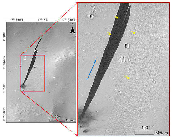
Figure 10.
New impact site that triggers a slope streak, as observed in the ESP_054066_1920 HiRISE image, which was acquired on 7 February 2018. The yellow arrows indicate the flow-parallel striations, which confirm a mass movement or fluidized flow in the dark streak and in a faded adjacent streak. The blue arrow indicates the direction of the flow. HiRISE image credit: NASA/JPL/University of Arizona.
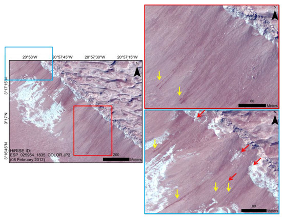
Figure 11.
Recurring slope lineae (RSL) in a hematite-rich area (red terrain) in Aureum Chaos as observed in HiRISE image ESP_025954_1835, which was acquired on 08 February 2012. Aureum Chaos is a major canyon system and the collapsed area is abundant in hydrated or clay minerals (phyllosilicates) and salts as a result of vast groundwater discharge in the past. Sulfate salts with magnesium, calcium, and iron are particularly predominant in this region. The red arrows highlight the spatial correlation between the salt-bearing deposits (white) on the slopes and the RSL features (yellow arrows) that are observed directly below them, while such features are missing on the slopes where salt-bearing deposits are not visible. HiRISE image credit: NASA/JPL/University of Arizona.
Another important observation that was made during the present research is that the fluidized phase in the Salar de Uyuni brines was transparent and the base terrain of the brines was clearly visible during the field work, which corresponds to the presence of majorly pure liquid phase in the brines and not only salt-hydrate complexes, thereby suggesting that a well-developed deliquescence mechanism is responsible for the formation of these brines. The brines in Salar de Uyuni have high concentrations of Ca2+ and Cl− ions [106] and CaCl2 can show very high eutectics at diurnal scales [55] in the temperature and RH conditions of Salar de Uyuni. CaCl2 should spontaneously dissolve into the liquid phase by deliquescence under such temperature and RH conditions; thus, the formed brines are abundant in a pure liquid phase that contains completely dissolved salt species and has high transparency. This further demonstrates the sequence of formation mechanisms of such terrestrial brines, in which the upper-crust salts on the higher slopes of EMZ initially undergo sapping or deliquescence via interaction with subsurface or atmospheric water, respectively, when the temperature and RH conditions are favorable. Subsequently, the produced pure liquid phase, after gaining enough volume, starts moving downslope, thereby facilitating the sapping/deliquescence of adjacent salty slopes and gradually increasing in dimensions throughout the brine season. Observing this transparency in brines from a UAV platform is important not only for demonstrating UAV’s usability for such research but also for confirming a large-scale deliquescence in a terrestrial environment, which may have implications for our understanding of similar extraterrestrial processes.
5. Conclusions
The present research explores the short-term intra-seasonal terrain changes of the briny salt flat environment at unprecedented spatial resolutions using UAVs and makes analogous inferences with implications for proposed Martian brines. We have provided detailed information on a methodology for obtaining topographical data, which may also be helpful for other researchers in UAV flight planning and execution. The use of UAVs for temporal monitoring of such salt flats can improve our knowledge about nutrient transport across the salt flat mixing zones, precise modeling of ecological vulnerability, and mineralogical estimations. Such high-resolution and UAV-based geomorphometric mapping of salt flat brines had never been performed before and the results of the present study demonstrate the high diurnal dynamism in these seasonal brines and further provide important inferences for several unresolved issues that are related to understanding the proposed Martian brines. For example, the absence of observable topographic relief or terrain perturbations within most of the proposed Martian brines appears to be more of an issue related to the remote sensor’s spatial resolution limits than the actual absence of erosion and deposition features within or around the proposed Martian brines, demonstrating the possibility of fluidized flows within the Martian surface features that are projected as Martian brines. The dependence of the rate of terrain change within the Salar brines on the slope and size of the brines further explains the wide dimensional and topographical variabilities that are observed in the proposed Martian brines.
Here, we established Salar de Uyuni as a more suitable terrestrial analogue for the proposed Martian brines than the previously published analogues from Dry Valleys, Antarctica due to Salar’s location outside permafrost or snowy terrain in a cold arid environment. It is easier to reach Salar de Uyuni and conduct analogous brine research. Thus, we expect the present research to motivate future studies in this direction. In addition, in the present paper, our focus is primarily to discuss the brine analogy between salt flats on Earth and salty terrain on Mars. However, such salt flats in South America can be extremely useful for establishing many geological e.g., [48,111,112] and astrobiological e.g., [113,114] analogies. For example, as a future prospect, analogous research between the salt desiccation polygons in Salar de Uyuni and the cracks that are found in a recently discovered evaporated salt pond on Mars [115] (Figure 12) can be established to model the landscape evolution in such salt flats. In addition, the morphological differences between the polygons in the same image frame, as shown in the insets of Figure 12b, can further be established as an indicator of minute groundwater level differences that arise from differential flow rates and mixing [32] within the salt flats at local scales. With the advent of hyperspectral cameras that are mountable on UAVs, the next step in brine analogue research can be to monitor the changing mineralogy and hydration levels of such terrestrial brines and their surroundings throughout the season to reveal the mystery behind the differential hydration levels that are observed within and around the proposed Martian brines. Due to logistic issues, a detailed investigation on the absolute DEM accuracy was not possible during the present field work. However, we later tried to estimate the absolute positional accuracy of the generated DEM for our UAV system with respect to the Trimble R10 Integrated Differential Global Navigation Satellite System (DGNSS) for a flat test area as the study area. The obtained root mean square error (RMSE) was ~7 m in vertical and ~2 m in horizontal without using any GCP and solely relying on the GPS onboard the UAV; sufficient enough for our objectives, which mainly focused on imaging and observing dimensional changes in the streaks and were independent of the requirement of the absolute positional accuracy. Yet, our use of SGCPs provides better confidence to the obtained results and inferences. This range of RMSE is reported by another recent study [116] for the similar UAV systems. Seasonal monitoring of such brine environments over several years can reveal at high resolution the impact of the changing climate on the hydrology and groundwater dynamics of these ecologically vulnerable regions. It will also be advantageous to add inferences based on numerical simulations consisting of considerations for Martian gravity to derive possible regolith transports within the expected Martian brines.
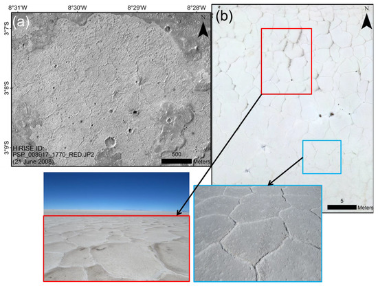
Figure 12.
Salt desiccation polygons on Earth and Mars. (a) Salt evaporites and polygonal salt cracks near Meridiani Planum, Mars. (b) Salt desiccation polygons in Salar de Uyuni, as captured using UAV. The Martian salt cracks are nearly two orders of magnitude larger than the Salar cracks. Field photograph credit: Group of Atmospheric Science, Luleå University of Technology. HiRISE image credit: NASA/JPL/University of Arizona.
Author Contributions
Conceptualization, A.B.; field data collection, A.B. and J.A.R.L.; data processing, A.B., L.S. and J.A.R.L.; formal analysis, A.B., L.S., F.J.M.-T. and M.-P.Z.; investigation, A.B., L.S., F.J.M.-T. and M.-P.Z.; methodology, A.B. and L.S.; software, A.B. and L.S.; writing—original draft, A.B.; writing—review and editing, L.S., F.J.M.-T. and M.-P.Z.
Funding
This research received no external funding.
Acknowledgments
We thank the efforts of the guest editor and the reviewers for their suggestions in improving the paper. We acknowledge the Wallenberg Foundation and the Kempe Foundation for supporting our Mars research activities in general. We thank NASA, JPL, and University of Arizona for providing HiRISE images free of charge. The maps in various figures have been created using ArcGIS version 10.6.1.
Conflicts of Interest
The authors declare no conflicts of interest. The funders had no role in the design of the study; in the collection, analyses, or interpretation of data; in the writing of the manuscript, or in the decision to publish the results.
References
- Bhardwaj, A.; Sam, L.; Akanksha; Martín-Torres, F.J.; Kumar, R. UAVs as remote sensing platform in glaciology: Present applications and future prospects. Remote Sens. Environ. 2016, 175, 196–204. [Google Scholar] [CrossRef]
- Colomina, I.; Molina, P. Unmanned aerial systems for photogrammetry and remote sensing: A review. ISPRS J. Photogramm. Remote Sens. 2014, 92, 79–97. [Google Scholar] [CrossRef]
- Aasen, H.; Burkart, A.; Bolten, A.; Bareth, G. Generating 3D hyperspectral information with lightweight UAV snapshot cameras for vegetation monitoring: From camera calibration to quality assurance. ISPRS J. Photogramm. Remote Sens. 2015, 108, 245–259. [Google Scholar] [CrossRef]
- Gago, J.; Douthe, C.; Coopman, R.; Gallego, P.; Ribas-Carbo, M.; Flexas, J.; Escalona, J.; Medrano, H. UAVs challenge to assess water stress for sustainable agriculture. Agric. Water Manag. 2015, 153, 9–19. [Google Scholar] [CrossRef]
- Luna, I.; Lobo, A. Mapping Crop Planting Quality in Sugarcane from UAV Imagery: A Pilot Study in Nicaragua. Remote Sens. 2016, 8, 500. [Google Scholar] [CrossRef]
- Chianucci, F.; Disperati, L.; Guzzi, D.; Bianchini, D.; Nardino, V.; Lastri, C.; Rindinella, A.; Corona, P. Estimation of canopy attributes in beech forests using true colour digital images from a small fixed-wing UAV. Int. J. Appl. Earth Obs. Geoinf. 2016, 47, 60–68. [Google Scholar] [CrossRef]
- Getzin, S.; Nuske, R.S.; Wiegand, K. Using Unmanned Aerial Vehicles (UAV) to Quantify Spatial Gap Patterns in Forests. Remote Sens. 2014, 6, 6988–7004. [Google Scholar] [CrossRef]
- Goldbergs, G.; Maier, S.W.; Levick, S.R.; Edwards, A. Efficiency of Individual Tree Detection Approaches Based on Light-Weight and Low-Cost UAS Imagery in Australian Savannas. Remote Sens. 2018, 10, 161. [Google Scholar] [CrossRef]
- Mikita, T.; Janata, P.; Surový, P. Forest Stand Inventory Based on Combined Aerial and Terrestrial Close-Range Photogrammetry. Forests 2016, 7, 165. [Google Scholar] [CrossRef]
- Wallace, L.; Lucieer, A.; Malenovský, Z.; Turner, D.; Vopěnka, P. Assessment of Forest Structure Using Two UAV Techniques: A Comparison of Airborne Laser Scanning and Structure from Motion (SfM) Point Clouds. Forests 2016, 7, 62. [Google Scholar] [CrossRef]
- Koeva, M.; Muneza, M.; Gevaert, C.; Gerke, M.; Nex, F. Using UAVs for map creation and updating. A case study in Rwanda. Surv. Rev. 2018, 50, 312–325. [Google Scholar] [CrossRef]
- Clapuyt, F.; Vanacker, V.; Van Oost, K. Reproducibility of UAV-based earth topography reconstructions based on Structure-from-Motion algorithms. Geomorphology 2016, 260, 4–15. [Google Scholar] [CrossRef]
- Flynn, K.F.; Chapra, S.C. Remote Sensing of Submerged Aquatic Vegetation in a Shallow Non-Turbid River Using an Unmanned Aerial Vehicle. Remote Sens. 2014, 6, 12815–12836. [Google Scholar] [CrossRef]
- Liu, T.; Abd-Elrahman, A.; Morton, J.; Wilhelm, V.L.; Jon, M. Comparing fully convolutional networks, random forest, support vector machine, and patch-based deep convolutional neural networks for object-based wetland mapping using images from small unmanned aircraft system. GISci. Remote Sens. 2018, 55, 243–264. [Google Scholar] [CrossRef]
- Smith, M.W.; Carrivick, J.L.; Quincey, D.J. Structure from motion photogrammetry in physical geography. Prog. Phys. Geogr. 2016, 40, 247–275. [Google Scholar] [CrossRef]
- Iizuka, K.; Itoh, M.; Shiodera, S.; Matsubara, T.; Dohar, M.; Watanabe, K. Advantages of unmanned aerial vehicle (UAV) photogrammetry for landscape analysis compared with satellite data: A case study of postmining sites in Indonesia. Cogent Geosci. 2018, 4, 1–15. [Google Scholar] [CrossRef]
- Tong, X.; Liu, X.; Chen, P.; Liu, S.; Luan, K.; Li, L.; Liu, S.; Liu, X.; Xie, H.; Jin, Y.; et al. Integration of UAV-Based Photogrammetry and Terrestrial Laser Scanning for the Three-Dimensional Mapping and Monitoring of Open-Pit Mine Areas. Remote Sens. 2015, 7, 6635–6662. [Google Scholar] [CrossRef]
- Turner, D.; Lucieer, A.; De Jong, S.M. Time Series Analysis of Landslide Dynamics Using an Unmanned Aerial Vehicle (UAV). Remote Sens. 2015, 7, 1736–1757. [Google Scholar] [CrossRef]
- De Reu, J.; De Smedt, P.; Herremans, D.; Van Meirvenne, M.; Laloo, P.; De Clercq, W. On introducing an image-based 3D reconstruction method in archaeological excavation practice. J. Archaeol. Sci. 2014, 41, 251–262. [Google Scholar] [CrossRef]
- Storlazzi, C.D.; Dartnell, P.; Hatcher, G.A.; Gibbs, A.E. End of the chain? Rugosity and fine-scale bathymetry from existing underwater digital imagery using structure-from-motion (SfM) technology. Coral Reefs 2016, 35, 889–894. [Google Scholar] [CrossRef]
- Jaud, M.; Grasso, F.; Le Dantec, N.; Verney, R.; Delacourt, C.; Ammann, J.; Deloffre, J.; Grandjean, P. Potential of UAVs for Monitoring Mudflat Morphodynamics (Application to the Seine Estuary, France). ISPRS Int. J. Geo-Inf. 2016, 5, 50. [Google Scholar] [CrossRef]
- Long, N.; Millescamps, B.; Guillot, B.; Pouget, F.; Bertin, X. Monitoring the Topography of a Dynamic Tidal Inlet Using UAV Imagery. Remote Sens. 2016, 8, 387. [Google Scholar] [CrossRef]
- Kalacska, M.; Chmura, G.; Lucanus, O.; Bérubé, D.; Arroyo-Mora, J. Structure from motion will revolutionize analyses of tidal wetland landscapes. Remote Sens. Environ. 2017, 199, 14–24. [Google Scholar] [CrossRef]
- Hardin, P.J.; Jensen, R.R. Small-Scale Unmanned Aerial Vehicles in Environmental Remote Sensing: Challenges and Opportunities. GISci. Remote Sens. 2011, 48, 99–111. [Google Scholar] [CrossRef]
- Nex, F.; Remondino, F. UAV for 3D mapping applications: A review. Appl. Geomat. 2013, 6, 1–15. [Google Scholar] [CrossRef]
- Watts, A.C.; Ambrosia, V.G.; Hinkley, E.A. Unmanned Aircraft Systems in Remote Sensing and Scientific Research: Classification and Considerations of Use. Remote Sens. 2012, 4, 1671–1692. [Google Scholar] [CrossRef]
- Whitehead, K.; Hugenholtz, C.H. Remote sensing of the environment with small unmanned aircraft systems (UASs), part 1: A review of progress and challenges. J. Unmanned Veh. Syst. 2014, 2, 69–85. [Google Scholar] [CrossRef]
- Milewski, R.; Chabrillat, S.; Behling, R. Analyses of Recent Sediment Surface Dynamic of a Namibian Kalahari Salt Pan Based on Multitemporal Landsat and Hyperspectral Hyperion Data. Remote Sens. 2017, 9, 170. [Google Scholar] [CrossRef]
- Svendsen, J.B. Parabolic halite dunes on the Salar de Uyuni, Bolivia. Sediment. Geol. 2003, 155, 147–156. [Google Scholar] [CrossRef]
- Belnap, J.; Munson, S.M.; Field, J.P. Aeolian and fluvial processes in dryland regions: The need for integrated studies. Ecohydrology 2011, 4, 615–622. [Google Scholar] [CrossRef]
- USGS. Mineral Commodities Summary. 2017. Available online: https://minerals.usgs.gov/minerals/pubs/mcs/ (accessed on 5 December 2018).
- Marazuela, M.; Vázquez-Suñè, E.; Custodio, E.; Palma, T.; Garcia-Gil, A.; Ayora, C. 3D mapping, hydrodynamics and modelling of the freshwater-brine mixing zone in salt flats similar to the Salar de Atacama (Chile). J. Hydrol. 2018, 561, 223–235. [Google Scholar] [CrossRef]
- Dieng, N.M.; Dinis, J.; Faye, S.; Gonçalves, M.; Caetano, M. Combined Uses of Supervised Classification and Normalized Difference Vegetation Index Techniques to Monitor Land Degradation in the Saloum Saline Estuary System. In Estuaries of the World; Springer Science and Business Media LLC: Berlin/Heidelberg, Germany, 2014; pp. 49–63. [Google Scholar]
- Kumar, L.; Sinha, P. Mapping salt-marsh land-cover vegetation using high-spatial and hyperspectral satellite data to assist wetland inventory. GISci. Remote Sens. 2014, 51, 483–497. [Google Scholar] [CrossRef]
- Lee, Y.-K.; Park, J.-W.; Choi, J.-K.; Oh, Y.; Won, J.-S. Potential uses of TerraSAR-X for mapping herbaceous halophytes over salt marsh and tidal flats. Estuarine Coast. Shelf Sci. 2012, 115, 366–376. [Google Scholar] [CrossRef]
- Alphan, H.; Yilmaz, K.T.; Yılmaz, K.T. Monitoring Environmental Changes in the Mediterranean Coastal Landscape: The Case of Cukurova, Turkey. Environ. Manag. 2005, 35, 607–619. [Google Scholar] [CrossRef] [PubMed]
- Sun, C.; Liu, Y.; Zhao, S.; Zhou, M.; Yang, Y.; Li, F. Classification mapping and species identification of salt marshes based on a short-time interval NDVI time-series from HJ-1 optical imagery. Int. J. Appl. Earth Obs. Geoinf. 2016, 45, 27–41. [Google Scholar] [CrossRef]
- Shalaby, A.; Tateishi, R. Remote sensing and GIS for mapping and monitoring land cover and land-use changes in the Northwestern coastal zone of Egypt. Appl. Geogr. 2007, 27, 28–41. [Google Scholar] [CrossRef]
- Silvestri, S.; Marani, M.; Marani, A. Hyperspectral remote sensing of salt marsh vegetation, morphology and soil topography. Phys. Chem. Earth Parts A/B/C 2003, 28, 15–25. [Google Scholar] [CrossRef]
- Kourkouli, P.; Wegmüller, U.; Teatini, P.; Tosi, L.; Strozzi, T.; Wiesmann, A.; Tansey, K. Ground Deformation Monitoring Over Venice Lagoon Using Combined DInSAR/PSI Techniques. In Engineering Geology for Society and Territory Volume 4; Springer Science and Business Media LLC: Berlin/Heidelberg, Germany, 2014; pp. 183–186. [Google Scholar]
- Kampf, S.K.; Tyler, S.W.; Ortiz, C.A.; Muñoz, J.F.; Adkins, P.L. Evaporation and land surface energy budget at the Salar de Atacama, Northern Chile. J. Hydrol. 2005, 310, 236–252. [Google Scholar] [CrossRef]
- Turk, L. Diurnal fluctuations of water tables induced by atmospheric pressure changes. J. Hydrol. 1975, 26, 1–16. [Google Scholar] [CrossRef]
- Mason, J.L.; Kipp, K.L. Hydrology of the Bonneville Salt Flats, Northwestern Utah, and Simulation of Gound-Water Flow and Solute Transport in the Shallow-Brine Aquifer; United States Geological Professional Paper 1585; U.S. Geological Survey: Denver, CO, USA, 1997.
- Kesler, S.E.; Gruber, P.W.; Medina, P.A.; Keoleian, G.A.; Everson, M.P.; Wallington, T.J. Global lithium resources: Relative importance of pegmatite, brine and other deposits. ORE Geol. Rev. 2012, 48, 55–69. [Google Scholar] [CrossRef]
- Goudie, A.S.; Watson, A. Rock block monitoring of rapid salt weathering in southern Tunisia. Earth Surf. Process. Landf. 1984, 9, 95–98. [Google Scholar] [CrossRef]
- White, W.W., III. Salt Laydown Project-Replenishment of salt to the Bonneville Salt Flats. In Great Salt Lake-An Overview of Change: Special Publication of the Utah Department of Natural Resources; Utah Geological Survey: Salt Lake City, UT, USA, 2002; pp. 433–486. [Google Scholar]
- Rosen, M.R. The Importance of Groundwater in Playas: A Review of Playa Classifications and the Sedimentology and Hydrology of Playas. Geol. Soc. Am. Spec. Pap. 1994, 289, 1–18. [Google Scholar] [CrossRef]
- El-Maarry, M.R.; Watters, W.A.; Yoldi, Z.; Pommerol, A.; Fischer, D.; Eggenberger, U.; Thomas, N. Dried Lakes in Western United States as Analogue to Desiccation Fractures on Mars. In Proceedings of the 47th Lunar and Planetary Science Conference, The Woodlands, TX, USA, 21–25 March 2016. [Google Scholar]
- El-Maarry, M.R.; Pommerol, A.; Thomas, N. Desiccation of phyllosilicate-bearing samples as analog for desiccation cracks on Mars: Experimental setup and initial results. Planet. Space Sci. 2015, 111, 134–143. [Google Scholar] [CrossRef]
- Edwards, H.G.M.; Mohsin, M.A.; Sadooni, F.N.; Hassan, N.F.N.; Munshi, T. Life in the sabkha: Raman spectroscopy of halotrophic extremophiles of relevance to planetary exploration. Anal. Bioanal. Chem. 2006, 385, 46–56. [Google Scholar] [CrossRef] [PubMed]
- Bhardwaj, A.; Sam, L.; Martín-Torres, F.J.; Zorzano, M.-P. Are Slope Streaks Indicative of Global-Scale Aqueous Processes on Contemporary Mars? Rev. Geophys. 2019, 57, 48–77. [Google Scholar] [CrossRef]
- Bhardwaj, A.; Sam, L.; Martín-Torres, F.J.; Zorzano, M.-P. Revisiting Enigmatic Martian Slope Streaks. EOS 2019, 100. [Google Scholar] [CrossRef]
- McEwen, A.S.; Ojha, L.; Dundas, C.M.; Mattson, S.S.; Byrne, S.; Wray, J.J.; Cull, S.C.; Murchie, S.L.; Thomas, N.; Gulick, V.C. Seasonal Flows on Warm Martian Slopes. Science 2011, 333, 740–743. [Google Scholar] [CrossRef]
- Ojha, L.; Wilhelm, M.B.; Murchie, S.L.; McEwen, A.S.; Wray, J.J.; Hanley, J.; Massé, M.; Chojnacki, M.; Chojnacki, M. Spectral evidence for hydrated salts in recurring slope lineae on Mars. Nat. Geosci. 2015, 8, 829–832. [Google Scholar] [CrossRef]
- Bhardwaj, A.; Sam, L.; Martín-Torres, F.J.; Zorzano, M.-P.; Fonseca, R.M. Martian slope streaks as plausible indicators of transient water activity. Sci. Rep. 2017, 7, 7074. [Google Scholar] [CrossRef]
- Head, J.W.; Marchant, D.R.; Dickson, J.L.; Levy, J.S.; Morgan, G.A. Slope Streaks in the Antarctic Dry Valleys: Characteristics, Candidate Formation Mechanisms, and Implications for Slope Streak Formation in the Martian Environment; U.S. Geological Survey: Denver, CO, USA, 2007.
- Kreslavsky, M.A.; Head, J.W. Slope streaks on Mars: A new “wet” mechanism. Icarus 2009, 201, 517–527. [Google Scholar] [CrossRef]
- Rettberg, P.; Anesio, A.M.; Baker, V.R.; Baross, J.A.; Cady, S.L.; Detsis, E.; Foreman, C.M.; Hauber, E.; Ori, G.G.; Pearce, D.A.; et al. Planetary Protection and Mars Special Regions—A Suggestion for Updating the Definition. Astrobiology 2016, 16, 119–125. [Google Scholar] [CrossRef] [PubMed]
- Rummel, J.D. Special regions in Mars exploration: Problems and potential. Acta Astronaut. 2009, 64, 1293–1297. [Google Scholar] [CrossRef]
- Rummel, J.D.; Beaty, D.W.; Jones, M.A.; Bakermans, C.; Barlow, N.G.; Boston, P.J.; Chevrier, V.F.; Clark, B.C. de Vera Jean-Pierre, P.; Gough, R.V.; et al. A new analysis of Mars “special regions”: Findings of the second MEPAG Special Regions Science Analysis Group (SR-SAG2). Astrobiology 2014, 14, 887–968. [Google Scholar] [CrossRef] [PubMed]
- Chevrier, V.F.; Rivera-Valentin, E.G. Formation of recurring slope lineae by liquid brines on present-day Mars. Geophys. Res. Lett. 2012, 39. [Google Scholar] [CrossRef]
- Levy, J. Hydrological characteristics of recurrent slope lineae on Mars: Evidence for liquid flow through regolith and comparisons with Antarctic terrestrial analogs. Icarus 2012, 219, 1–4. [Google Scholar] [CrossRef]
- Mitchell, J.L.; Christensen, P.R. Recurring slope lineae and chlorides on the surface of Mars. J. Geophys. Res. Planets 2016, 121, 1411–1428. [Google Scholar] [CrossRef]
- Stillman, D.E.; Michaels, T.I.; Grimm, R.E.; Harrison, K.P. New observations of Martian southern mid-latitude recurring slope lineae (RSL) imply formation by freshwater subsurface flows. Icarus 2014, 233, 328–341. [Google Scholar] [CrossRef]
- Stillman, D.E.; Michaels, T.I.; Grimm, R.E.; Hanley, J. Observations and modeling of northern mid-latitude recurring slope lineae (RSL) suggest recharge by a present-day martian briny aquifer. Icarus 2016, 265, 125–138. [Google Scholar] [CrossRef]
- Schmidt, F.; Andrieu, F.; Costard, F.; Kocifaj, M.; Meresescu, A.G. Formation of recurring slope lineae on Mars by rarefied gas-triggered granular flows. Nat. Geosci. 2017, 10, 270–273. [Google Scholar] [CrossRef]
- Dundas, C.M.; McEwen, A.S.; Chojnacki, M.; Milazzo, M.P.; Byrne, S.; McElwaine, J.N.; Urso, A. Granular flows at recurring slope lineae on Mars indicate a limited role for liquid water. Nat. Geosci. 2017, 10, 903–907. [Google Scholar] [CrossRef]
- Masse, M.; Conway, S.J.; Gargani, J.; Patel, M.R.; Pasquon, K.; McEwen, A.; Carpy, S.; Chévrier, V.; Balme, M.R.; Ojha, L.; et al. Transport processes induced by metastable boiling water under Martian surface conditions. Nat. Geosci. 2016, 9, 425–428. [Google Scholar] [CrossRef]
- Chojnacki, M.; McEwen, A.; Dundas, C.; Ojha, L.; Urso, A.; Sutton, S. Geologic context of recurring slope lineae in Melas and Coprates Chasmata, Mars. J. Geophys. Res. Planets 2016, 121, 1204–1231. [Google Scholar] [CrossRef]
- Edwards, C.S.; Piqueux, S. The water content of recurring slope lineae on Mars. Geophys. Res. Lett. 2016, 43, 8912–8919. [Google Scholar] [CrossRef]
- Grimm, R.E.; Harrison, K.P.; Stillman, D.E. Water budgets of martian recurring slope lineae. Icarus 2014, 233, 316–327. [Google Scholar] [CrossRef]
- Mars Helicopter to Fly on NASA’s Next Red Planet Rover Mission. Available online: https://www.nasa.gov/press-release/mars-helicopter-to-fly-on-nasa-s-next-red-planet-rover-mission (accessed on 5 June 2019).
- Risacher, F.; Alonso, H.; Salazar, C. The origin of brines and salts in Chilean salars: A hydrochemical review. Earth-Sci. Rev. 2003, 63, 249–293. [Google Scholar] [CrossRef]
- Baker, P.A.; Rigsby, C.A.; Seltzer, G.O.; Fritz, S.C.; Lowenstein, T.K.; Bacher, N.P.; Veliz, C. Tropical climate changes at millennial and orbital timescales on the Bolivian Altiplano. Nature 2001, 409, 698–701. [Google Scholar] [CrossRef]
- Lamparelli, R.C.; Ponzoni, F.; Zullo, J.; Pellegrino, G.Q.; Arnaud, Y. Characterization of the salar de uyuni for in-orbit satellite calibration. IEEE Trans. Geosci. Remote Sens. 2003, 41, 1461–1468. [Google Scholar] [CrossRef]
- Gush, W.G. The Decline of the Globally Threatened Rudd’s Lark in One of Its Last Remaining Core Sites, the Wakkerstroom Grasslands. Ph.D. Thesis, University of Cape Town, Cape Town, South Africa, 2017. Available online: https://open.uct.ac.za/handle/11427/25011 (accessed on 31 August 2018).
- Jones, K. An Inventory and Mapping of Cliffs within the South Cumberland Plateau Region of Tennessee. Master’s Thesis, The University of Tennessee at Chattanooga, Chattanooga, TN, USA, May 2018. Available online: https://scholar.utc.edu/theses/562/ (accessed on 31 August 2018).
- Lindstrøm, I.M. No Mitigating Effects of Roadside Vegetation Clearing on Ungulate-Vehicle Collisions in Nord-Trøndelag. Master’s Thesis, Norwegian University of Science and Technology (NTNU), Trondheim, Norway, 2016. Available online: https://brage.bibsys.no/xmlui/handle/11250/2391557 (accessed on 31 August 2018).
- Tussadiah, A.; Subandriyo, J.; Novita, S.; Pranowo, W.S. Verification of Pisces Dissolved Oxygen Model Using in Situ Measurement in Biak, Rote, And Tanimbar Seas, Indonesia. Int. J. Remote Sens. Earth Sci. (IJReSES) 2017, 14, 37–46. [Google Scholar] [CrossRef][Green Version]
- Ullman, S. The interpretation of structure from motion. Proc. R. Soc. Lond. Ser. B Boil. Sci. 1979, 203, 405–426. [Google Scholar]
- Sona, G.; Pinto, L.; Pagliari, D.; Passoni, D.; Gini, R. Experimental analysis of different software packages for orientation and digital surface modelling from UAV images. Earth Sci. Inform. 2014, 7, 97–107. [Google Scholar] [CrossRef]
- Burns, J.; Delparte, D.; Gates, R.; Takabayashi, M. Integrating structure-from-motion photogrammetry with geospatial software as a novel technique for quantifying 3D ecological characteristics of coral reefs. PeerJ 2015, 3, e1077. [Google Scholar] [CrossRef]
- Kersten, T.P.; Lindstaedt, M. Image-based low-cost systems for automatic 3D recording and modelling of archaeological finds and objects. In Euro-Mediterranean Conference; Springer: Berlin/Heidelberg, Germany, 2012; pp. 1–10. [Google Scholar]
- Themistocleous, K.; Ioannides, M.; Agapiou, A.; Hadjimitsis, D.G. The methodology of documenting cultural heritage sites using photogrammetry, UAV, and 3D printing techniques: The case study of Asinou Church in Cyprus. In Third International Conference on Remote Sensing and Geoinformation of the Environment (RSCy2015); International Society for Optics and Photonics: Bellingham, WA, USA, 2015; Volume 9535, p. 953510. [Google Scholar]
- Verhoeven, G. Software review taking computer vision aloft—Archaeological three-dimensional reconstructions from aerial photographs with PhotoScan. Archaeol. Prospect. 2011, 73, 67–73. [Google Scholar] [CrossRef]
- Furukawa, Y.; Ponce, J. Accurate Camera Calibration from Multi-View Stereo and Bundle Adjustment. Int. J. Comput. Vis. 2009, 84, 257–268. [Google Scholar] [CrossRef]
- Sam, L.; Bhardwaj, A.; Singh, S.; Kumar, R. Remote sensing flow velocity of debris-covered glaciers using Landsat 8 data. Prog. Phys. Geogr. 2016, 40, 305–321. [Google Scholar] [CrossRef]
- Sam, L.; Bhardwaj, A.; Kumar, R.; Buchroithner, M.F.; Martín-Torres, F.J. Heterogeneity in topographic control on velocities of Western Himalayan glaciers. Sci. Rep. 2018, 8, 12843. [Google Scholar] [CrossRef]
- Singh, M.K.; Snehmani Gupta, R.D.; Bhardwaj, A.; Joshi, P.K.; Ganju, A. High resolution DEM generation for complex and snow covered Indian Himalayan region using ADS80 Aerial Push-broom camera: A first time attempt. Arab. J. Geosci. 2015, 8, 1403–1414. [Google Scholar] [CrossRef]
- Singh, M.K.; Gupta, R.D.; Snehmani Bhardwaj, A.; Ganju, A. Scenario-based validation of moderate resolution DEMs freely available for complex Himalayan terrain. Pure Appl. Geophys. 2016, 173, 463–485. [Google Scholar] [CrossRef]
- Snehmani Bhardwaj, A.; Pandit, A.; Ganju, A. Demarcation of potential avalanche sites using remote sensing and ground observations: A case study of Gangotri glacier. Geocarto Int. 2014, 29, 520–535. [Google Scholar] [CrossRef]
- Burrough, P.A.; McDonell, R.A. Principles of Geographical Information Systems; Oxford University Press: Oxford, UK, 1998; p. 190. [Google Scholar]
- Moore, I.D.; Grayson, R.B.; Landson, A.R. Digital Terrain Modelling: A Review of Hydrological, Geomorphological, and Biological Applications. Hydrol. Process. 1991, 5, 3–30. [Google Scholar] [CrossRef]
- Zevenbergen, L.W.; Thorne, C.R. Quantitative analysis of land surface topography. Earth Surf. Process. Landf. 1987, 12, 47–56. [Google Scholar] [CrossRef]
- Wilson, M.F.J.; O’Connell, B.; Brown, C.; Guinan, J.C.; Grehan, A.J. Multiscale Terrain Analysis of Multibeam Bathymetry Data for Habitat Mapping on the Continental Slope. Mar. Geodesy 2007, 30, 3–35. [Google Scholar] [CrossRef]
- De Smith, M.J.; Goodchild, M.F.; Longley, P. Geospatial Analysis: A Comprehensive Guide to Principles, Techniques and Software Tools; Troubador Publishing Ltd.: Leicester, UK, 2007. [Google Scholar]
- Etzelmüller, B. On the Quantification of Surface Changes using Grid-based Digital Elevation Models (DEMs). Trans. GIS 2000, 4, 129–143. [Google Scholar] [CrossRef]
- Brusnikin, E.S.; Kreslavsky, M.A.; Zubarev, A.E.; Patratiy, V.D.; Krasilnikov, S.S.; Head, J.W.; Karachevtseva, I.P. Topographic measurements of slope streaks on Mars. Icarus 2016, 278, 52–61. [Google Scholar] [CrossRef]
- Abermann, J.; Fischer, A.; Lambrecht, A.; Geist, T. On the potential of very high-resolution repeat DEMs in glacial and periglacial environments. Cryosphere 2010, 4, 53–65. [Google Scholar] [CrossRef]
- Wang, D.; Kääb, A. Modeling Glacier Elevation Change from DEM Time Series. Remote Sens. 2015, 7, 10117–10142. [Google Scholar] [CrossRef]
- Dickson, J.L.; Head, J.W.; Levy, J.S.; Marchant, D.R. Don Juan Pond, Antarctica: Near-surface CaCl2-brine feeding Earth’s most saline lake and implications for Mars. Sci. Rep. 2013, 3, 1166. [Google Scholar] [CrossRef]
- Gough, R.; Wong, J.; Dickson, J.; Levy, J.; Head, J.; Marchant, D.; Tolbert, M. Brine formation via deliquescence by salts found near Don Juan Pond, Antarctica: Laboratory experiments and field observational results. Earth Planet. Sci. Lett. 2017, 476, 189–198. [Google Scholar] [CrossRef]
- Levy, J.S.; Fountain, A.G.; Gooseff, M.N.; Welch, K.A.; Lyons, W.B.; Gooseff, M. Water tracks and permafrost in Taylor Valley, Antarctica: Extensive and shallow groundwater connectivity in a cold desert ecosystem. GSA Bull. 2011, 123, 2295–2311. [Google Scholar] [CrossRef]
- Badgeley, J.A.; Pettit, E.C.; Carr, C.G.; Tulaczyk, S.; Mikucki, J.A.; Lyons, W.B. MIDGE Science Team An englacial hydrologic system of brine within a cold glacier: Blood Falls, McMurdo Dry Valleys, Antarctica. J. Glaciol. 2017, 63, 387–400. [Google Scholar] [CrossRef]
- Rangecroft, S.; Suggitt, A.J.; Anderson, K.; Harrison, S. Future climate warming and changes to mountain permafrost in the Bolivian Andes. Clim. Chang. 2016, 137, 231–243. [Google Scholar] [CrossRef]
- Risacher, F.; Fritz, B. Origin of salts and brine evolution of Bolivian and Chilean salars. Aquat. Geochem. 2009, 15, 123–157. [Google Scholar] [CrossRef]
- Chuang, F.C.; Beyer, R.A.; McEwen, A.S.; Thomson, B.J. HiRISE observations of slope streaks on Mars. Geophys. Res. Lett. 2007, 34. [Google Scholar] [CrossRef]
- Burleigh, K.J.; Melosh, H.J.; Tornabene, L.L.; Ivanov, B.; McEwen, A.S.; Daubar, I.J. Impact airblast triggers dust avalanches on Mars. Icarus 2012, 217, 194–201. [Google Scholar] [CrossRef]
- Bhardwaj, A.; Sam, L.; Martín-Torres, F.J.; Zorzano, M.-P. Discovery of recurring slope lineae candidates in Mawrth Vallis, Mars. Sci. Rep. 2019, 9, 2040. [Google Scholar] [CrossRef] [PubMed]
- Bhardwaj, A.; Sam, L.; Martin-Torres, F.J.; Zorzano, M.-P. Distribution and Morphologies of Transverse Aeolian Ridges in ExoMars 2020 Rover Landing Site. Remote Sens. 2019, 11, 912. [Google Scholar] [CrossRef]
- El-Maarry, M.R.; Pommerol, A.; Thomas, N. Analysis of polygonal cracking patterns in chloride-bearing terrains on Mars: Indicators of ancient playa settings. J. Geophys. Res. Planets 2013, 118, 2263–2278. [Google Scholar] [CrossRef]
- Hudson, T.L.; Aharonson, O. Diffusion barriers at Mars surface conditions: Salt crusts, particle size mixtures, and dust. J. Geophys. Res. Space Phys. 2008, 113. [Google Scholar] [CrossRef]
- Barbieri, R.; Stivaletta, N. Continental evaporites and the search for evidence of life on Mars. Geol. J. 2011, 46, 513–524. [Google Scholar] [CrossRef]
- Fairén, A.G.; Davila, A.F.; Lim, D.; Bramall, N.; Bonaccorsi, R.; Zavaleta, J.; Uceda, E.R.; Stoker, C.; Wierzchos, J.; Dohm, J.M.; et al. Astrobiology through the Ages of Mars: The Study of Terrestrial Analogues to Understand the Habitability of Mars. Astrobiology 2010, 10, 821–843. [Google Scholar] [CrossRef]
- Hynek, B.M.; Osterloo, M.K.; Kierein-Young, K.S. Late-stage formation of Martian chloride salts through ponding and evaporation. Geology 2015, 43, 787–790. [Google Scholar] [CrossRef]
- Manfreda, S.; Dvorak, P.; Mullerova, J.; Herban, S.; Vuono, P.; Justel, J.A.; Perks, M. Assessing the Accuracy of Digital Surface Models Derived from Optical Imagery Acquired with Unmanned Aerial Systems. Drones 2019, 3, 15. [Google Scholar] [CrossRef]


© 2019 by the authors. Licensee MDPI, Basel, Switzerland. This article is an open access article distributed under the terms and conditions of the Creative Commons Attribution (CC BY) license (http://creativecommons.org/licenses/by/4.0/).