Article

Estimation of the Maturity Date of Soybean Breeding Lines Using UAV-Based Multispectral Imagery

1
Division of Food Systems and Bioengineering, University of Missouri, Columbia, MO 65211, USA
2
Division of Plant Sciences, University of Missouri, Columbia, MO 65211, USA
*
Author to whom correspondence should be addressed.
Remote Sens. 2019, 11(18), 2075; https://doi.org/10.3390/rs11182075
Submission received: 6 August 2019 / Revised: 28 August 2019 / Accepted: 2 September 2019 / Published: 4 September 2019
(This article belongs to the Special Issue Advanced Imaging for Plant Phenotyping)

Abstract

:
Physiological maturity date is a critical parameter for the selection of breeding lines in soybean breeding programs. The conventional method to estimate the maturity dates of breeding lines uses visual ratings based on pod senescence by experts, which is subjective by human estimation, labor-intensive and time-consuming. Unmanned aerial vehicle (UAV)-based phenotyping systems provide a high-throughput and powerful tool of capturing crop traits using remote sensing, image processing and machine learning technologies. The goal of this study was to investigate the potential of predicting maturity dates of soybean breeding lines using UAV-based multispectral imagery. Maturity dates of 326 soybean breeding lines were taken using visual ratings from the beginning maturity stage (R7) to full maturity stage (R8), and the aerial multispectral images were taken during this period on 27 August, 14 September and 27 September, 2018. One hundred and thirty features were extracted from the five-band multispectral images. The maturity dates of the soybean lines were predicted and evaluated using partial least square regression (PLSR) models with 10-fold cross-validation. Twenty image features with importance to the estimation were selected and their changing rates between each two of the data collection days were calculated. The best prediction (R2 = 0.81, RMSE = 1.4 days) was made by the PLSR model using image features taken on 14 September and their changing rates between 14 September and 27 September with five components, leading to the conclusion that the UAV-based multispectral imagery is promising and practical in estimating maturity dates of soybean breeding lines.

Graphical Abstract

1. Introduction

By 2050, the global population is expected to reach 9.8 billion [1] and the current arable land is decreasing due to climate change, urbanization, soil degradation, water shortages and pollution [2]. Food demand is expected to be 60% higher than it is today resulting in global food supplies at a great stress. Crop breeding is a promising solution for the food crisis by developing new crop varieties with improved traits, including high yield potential and resilience to biotic and abiotic stresses due to adverse environments [3].
The rational of breeding programs is to select crop cultivars with superior genotypes among a large number of variants that have better production and quality, tolerance to biotic and abiotic stresses and high efficiency in cultivation, harvest and processing [4]. Selection criteria could be yield, lodging, flowering and maturity date, stress symptoms, severity, etc. depending on the purpose of breeding programs. Specifically in soybean breeding programs, physiological maturity date is a critical parameter for the selection of soybean lines. Soybeans with extended maturity time may take full advantage of the growing season to improve their yield [5]. However, soybeans in delayed harvest days may suffer frost damages or high harvest losses. Therefore, soybean cultivars are divided into maturity groups (MGs, e.g., MG III or MG IV) from 0 to 10 according to their time length from planting to physiological maturity, and also maturity group zones were developed to define where a soybean cultivar is the best [6].
Breeders determine the MG of a new variety by referring to the relative maturity (RM, by dividing a MG to 10 subgroups, e.g., RM3.0 to RM3.9 are 10 RMs in MG III) of the new variety to commercially released soybean cultivars (referred as checks) with a known MG. The relative maturity is determined by the differences in the maturity dates (the first day of the year when soybeans reach maturity status) between the new variety and the checks. Conventionally, soybean breeders take measurements of the physiological maturity date (R8) [7] of desired breeding lines using visual ratings by observing the pubescence color. However, visual rating is labor-intensive, time-consuming, and more importantly it is subjective [8]. In conventional breeding programs a breeder may need to scout tens of thousands of breeding lines in a progeny trail in a season [9], which makes it challenging to select the most desired lines. Therefore, there is a pressing need to develop an efficient and effective tool to take measurements of the maturity date of soybean progeny breeding lines in fields using novel approaches.
Maturity generally occurs when soybean pods have reached their physiological matured stages, showing gray, tan or brown color in pods [10]. After entering the beginning maturity stage (R7), the soybean plant, including leaves and pods, will lose moisture quickly from around 60% to less than 30%, depending on air temperature, humidity and soil conditions [11]. In addition, with the plant approaching senescence, the chlorophyll content of leaves reduces and color turns to yellow/gray [10], which might result in substantial changes in spectral reflectance. Therefore, it is possible to quantify the plant maturity level using the combinations of spectral reflectance in given wavebands that are very sensitive to crop canopy characteristics, such as chlorophyll content [12], nitrogen content and water stress [13].
Yu Li [9] developed a random forest model to classify mature and immature soybean lines using images in the blue and near-infrared band from an unmanned aerial vehicle (UAV)-based high-throughput phenotyping (HTP) platform, and achieved over 93% classification accuracy. Christenson Schapaugh [14] predicted relative maturity of soybean lines using a partial least square regression (PLSR) model with three vegetation indices (VIs) derived from narrow spectral bands that were acquired by a UAV imaging system. The correlation between predicted relative maturity and observed maturity was 0.5 with a root mean square error (RMSE) of 5.19 days. However, the difference between two relative maturity designations (e.g., RM 3.7 and RM 3.8) of soybeans is usually only one to two days (personal communication with a soybean breeder—Dr. Andrew Scaboo). It is not sufficient for soybean breeding purposes by classifying breeding lines into only two classes of mature and immature lines or the prediction with 5 days error. To the best of our knowledge, there is no studies showing such ability to determine accurate maturity date that breeders can use.
Therefore, the goal of this study was to investigate a method to estimate the maturity dates of soybean breeding lines using a UAV-based imaging system. There were three supportive objectives to achieve this goal: (1) To investigate the best time (growth stage) to collect images, (2) to select image features important to estimate relative maturity date and (3) to evaluate the estimation accuracy.

2. Materials and Methods

2.1. Field Experiment

The field experiment was conducted at an experimental field in the Greenley Research Center of the University of Missouri, Novelty, Missouri, United States (40°01′N, 92°11′W) in 2018. Eleven thousand, four hundred and seventy-three soybean lines were inbred from soybean varieties in MG III and IV, and planted on 29 May, 2018, in a 3.64 ha field. The soybean lines were planted in single-row plots, each being a progeny row derived from a single F4 plant, without replicates with 2.59 m in length and 0.76 m spacing in between rows. The breeding lines started maturing from September 19 and completed on 2 October, 2018.
Three hundred and twenty-six soybean lines were randomly selected before R8 stages as ground references for the estimation of maturity dates. The maturity dates of these soybean lines were determined by an experienced breeder using visual assessments. The measurements of maturity date were recorded every seven days starting from 31 August to 5 October. Mature plots were not observed until 19 September. In each measuring day, a soybean line that has approximately 95% of its pods achieved mature pod color was determined being mature and the date was recorded as its maturity date, and for those that have slightly less or more than 95% pods achieved mature color, the maturity dates were estimated as 1 to 3 days after or before the measuring day.

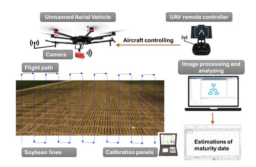
2.2. UAV Data Collection

Multispectral images were acquired using a multispectral camera RedEdge-M (MicaSense, Seattle, WA, USA) that has a resolution (number of total pixels) of 1260 pixels × 960 pixels. The details of wavelength are shown in Table 1. An iPad mini 3 (Apple Inc., Cupertino, CA, USA) was used to configure the camera taking time-lapse images at 1 frame per second (fps) by connecting the camera using its Wi-Fi hotspot. A GPS unit was attached to the camera and pre-programed to provide geo-referencing information for each frame of images. All images with the EXIF (Exchangeable Image File Format) metadata were saved to an onboard SD card of the camera. Before each flight, a calibration reflectance panel (CRP) was imaged by holding the camera at about 1 m above the CRP and looking vertically in an open area (to avoid shadow). The CRP has a factory calibrated reflectance in each of the five spectral bands that is used to convert the raw pixel values of multispectral images into reflectance during post processing [15]. The reflectance in each band of the CRP used in this study is shown in Table 1.
The multispectral camera was mounted on a UAV DJI Matrice 600 Pro (DJI, Shenzhen, China) with the camera facing to the ground vertically (nadir view). The UAV platform was controlled using a flight control App Autopilot (Hangar Technology, Austin, TX, U.S.A.) that allows setting up flight path, flying speed and elevation prior to the flights. Images were taken at 30 m above ground level (AGL) with a ground sample distance (GSD) of 20.8 mm∙pixel−1, and desired flight speed and number of paths were carefully determined to obtain sufficient overlaps (forward overlap of 87.5% and side overlap of 84.5% in this case) to cover the whole field. The images were acquired from 13:15:00 CDT to 15:00:00 CDT on 27 August, 14 September and 27 September, 2018.

2.3. Image Processing

The geo-referenced multispectral images were downloaded from the SD card and uploaded to a UAV image processing software Pix4D Mapper (Pix4D, Lausanne, Switzerland) to generate orthomosaic images of the field. After all the images were imported, the camera GPS information was read automatically from the EXIF metadata. The images of the CRP were selected and the reflectance was inputted manually following an instruction [16]. The “Ag Multispectral processing” template was chosen for this processing. When the processing was completed, the orthomosaic of each band was generated and exported as a .tif image, which was processed using the Image Processing Toolbox and Computer Vision System Toolbox of MATLAB (ver. 2016b, The MathWorks, Natick, MA, USA).
The background (soil and other non-crop) information was first removed from orthomosaic images using color thresholds. Figure 1a,c are the colorful images with the red (r), green (g) and blue (b) channels of images acquired on 27 August and 27 September and they show different color contrasts between soil and soybeans at different growth stages. A blue normalized difference vegetation index (BNDVI) [17] that could signify the crop pixels and suppress non-crop pixels was used to remove background of images on 27 August and 14 September as it had the highest contrast between soil and soybeans (Figure 1b). The blue-wide dynamic range vegetation index (BWDRVI) [18] was used for images on 27 September as it was found having higher contrast than BNDVI when soybean leaves started turning yellow and similar to soil color (Figure 1d). From the histograms in Figure 1e,f, pixels with BNDVI values higher than 0 or with BWDRVI values higher than 0.7 were considered as soybean lines.
B N D V I = n i r b l u e n i r + b l u e .
B W D R V I = 0.1 × n i r r e d 0.1 × n i r + r e d .
After background removal, individual soybean lines were segmented from one of the five-band images (the blue band images were used in this case) by manually drawing vertical and horizontal lines in alleys between plots. The segmented individual lines were saved as binary masks and then applied to the rest bands to get images of individual lines in each band. Each segmented line has a unique plot number associated according to its physical position in the field and the number was saved with images of the lines. The 326 soybean samples were recognized by matching plot numbers in ground reference data with those in segmented images.
Fifty-four vegetation indices (VIs) were extracted from the five-band images using the formula summarized by Agapiou Hadjimitsis [19] and Henrich Götze [20]. The formula and brief description of the selected VIs are included in the Appendix A Table A1. The mean and standard deviation (std) values of these Vis and the pixels of the five-band images of each single row were calculated as image features. In addition, we also calculated the mean and the std values of the hue, saturation (S) and value (V) in HSV color space and the L*, a* and b* in CIELAB color space, which were converted from r, g, and b channels using MATLAB function ‘rgb2hsv’ and ‘rgb2lab’. In total, 130 image features were extracted for further processing.

2.4. Maturity Date and Adjusted Maturity Date

The status of maturity was determined when approximately 95% of the pods in a line had achieved mature pod color by visual assessment [10], ignoring delayed leaf drop and green stems, which introduces variances in canopy images of soybean lines with the same maturity date. Additionally, maturity dates of soybean lines are usually determined visually by breeders in an interval of seven days and the dates of the breeding lines matured within the intervals were estimated based on experiences, therefore, the maturity dates may allow a one-or two-day error [9]. Figure 2 shows images of three soybean lines taken on 27 September. Although they were recorded with the maturity date of 25 September, they had different amount of green leaves remaining on the canopy. Line 7344 (left) had rarely leaves remaining so that it could be derived from the images that its pods have turned to mature color. However, certain amount of green leaves on the canopy of line 6913 (right) covered most of its stems. The real scenarios could be that either its pods had reached the mature color but with delayed dropping leaves or its maturity date was estimated too early in the interval of seven days.
In order to tolerate the variances in canopy leaves, we used a new parameter adjusted maturity date (adMD), calculated as Equation (3). The adMD calculates the variances in canopy images of the soybeans matured on the same day and applied the variances to the manually measured maturity date. The original maturity dates would be extended to a more precise format (22.2, 23.7 and 25.6 for soybean lines in Figure 2 from left to right) considering human error and canopy variances.
a d M D i = 1 n ( 1 n x i n m i n s t d i n ) + M D i ,
where adMDi is the adjusted maturity date of the ith soybean line. represents the ith soybean line, = 1, 2,…, 326 and n represents the nth image feature used in an estimation model, n = 1, 2,…, 130. MDi is the maturity date of the ith soybean line that is determined by breeders. xin is the value of the ith soybean line in the nth image feature. min is the mean of all soybean lines matured on the same day with the ith soybean line in the nth image features. stdin is the standard deviation of all soybean lines matured on the same day with the ith soybean line in the nth image features.

2.5. Data Analysis

All statistical analyses were conducted using the statistical toolboxes in MATLAB. To evaluate the potential of UAV-based imagery in estimating maturity dates, PLSR models were built using image features as predictors and maturity dates as responses for the data collected on three days. PLSR models create linear combinations (known as components) of the original predictor variables (image features) to explain the observed variability in the responses (measured maturity dates). Additionally, PLSR largely is able to reduce the variability and instability of estimated responses caused by multicollinearity among predictors [21]. The PLSR was conducted using ‘plsregress’ function with a 10-fold cross-validation. The estimation accuracy was evaluated using the RMSE of the estimated responses.
To develop a parsimonious and interpretable PLSR model for each data set, variable importance in projection (VIP) scores were used to select predictors by estimating the importance of each predictor in a PLSR model. A predictor with a VIP score close to or greater than 1 can be considered important in a given model [22]. The VIP scores of each predictor were calculated using MATLAB codes suggested by the MathWorks Support Team [23].
The variance inflation factor (VIF) was also calculated to remove image features with high collinearity [24]. The VIF is calculated as a dependent variable of the coefficient of determination (R2) of an individual feature against all other features. R2 was obtained by calling the parameter of ‘lm. Rsquare. Ordinary’ in the ‘fitlm’ function. This step was performed in a loop that the variable with the highest VIF was removed each time and the loop would not stop until the highest VIF is less or equal to 5 [25]. The higher the VIF value an image features have, the higher the collinearity is between this feature with others.
To better interpret the PLSR models, the correlation between each selected predictor and maturity dates were calculated using ‘corr’ function with the ‘Pearson’ option. As the multispectral images were collected on the three days at different growth stages of soybean lines, the changes in image features between each two days may indicate the transitions from the immature to mature status of soybean lines. The changing rate between each two data collection days was calculated using Equation (4).
C h a n g i n g   r a t e ( i ) = P ( i + 1 ) P ( i ) P ( i ) .
where P is each selected predictor of single soybean lines on the = 1st, 2nd and 3rd time of data collection.

3. Results

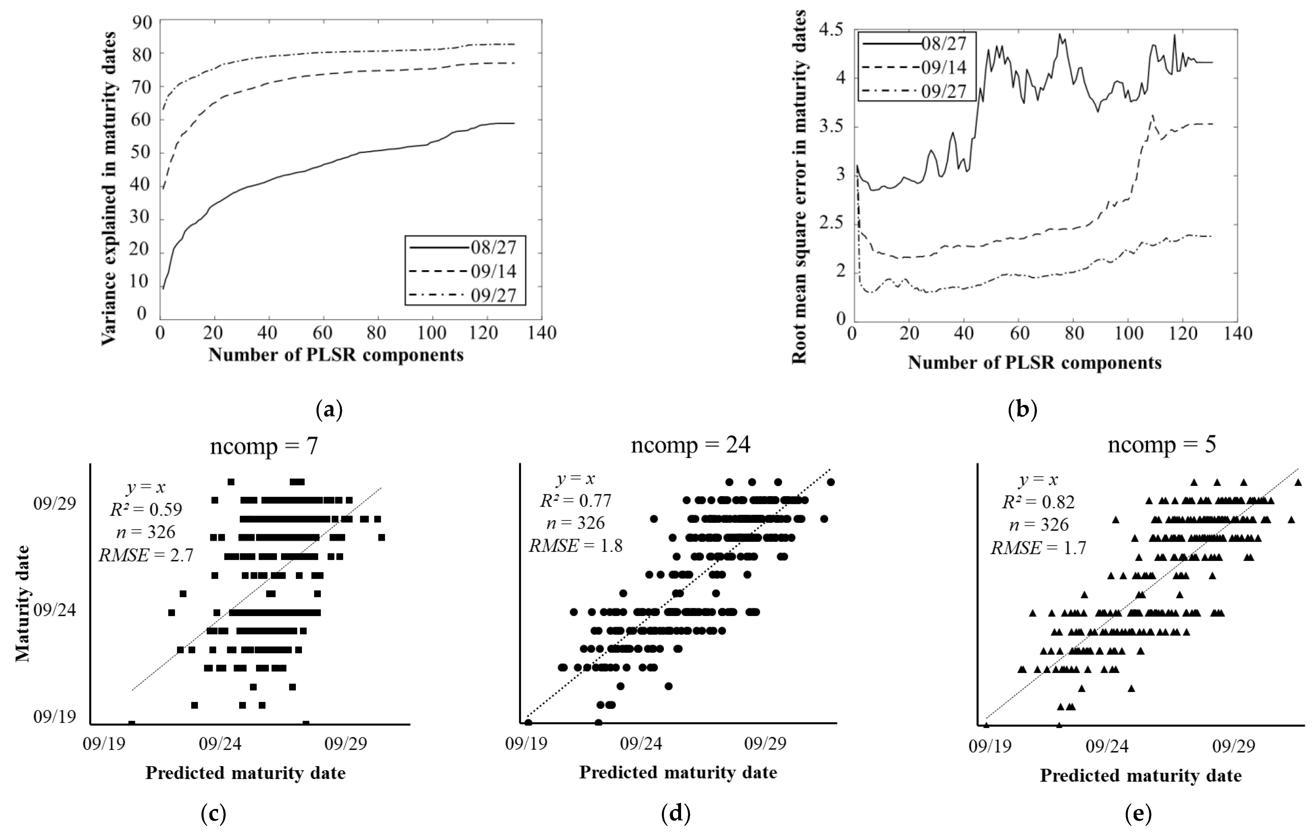
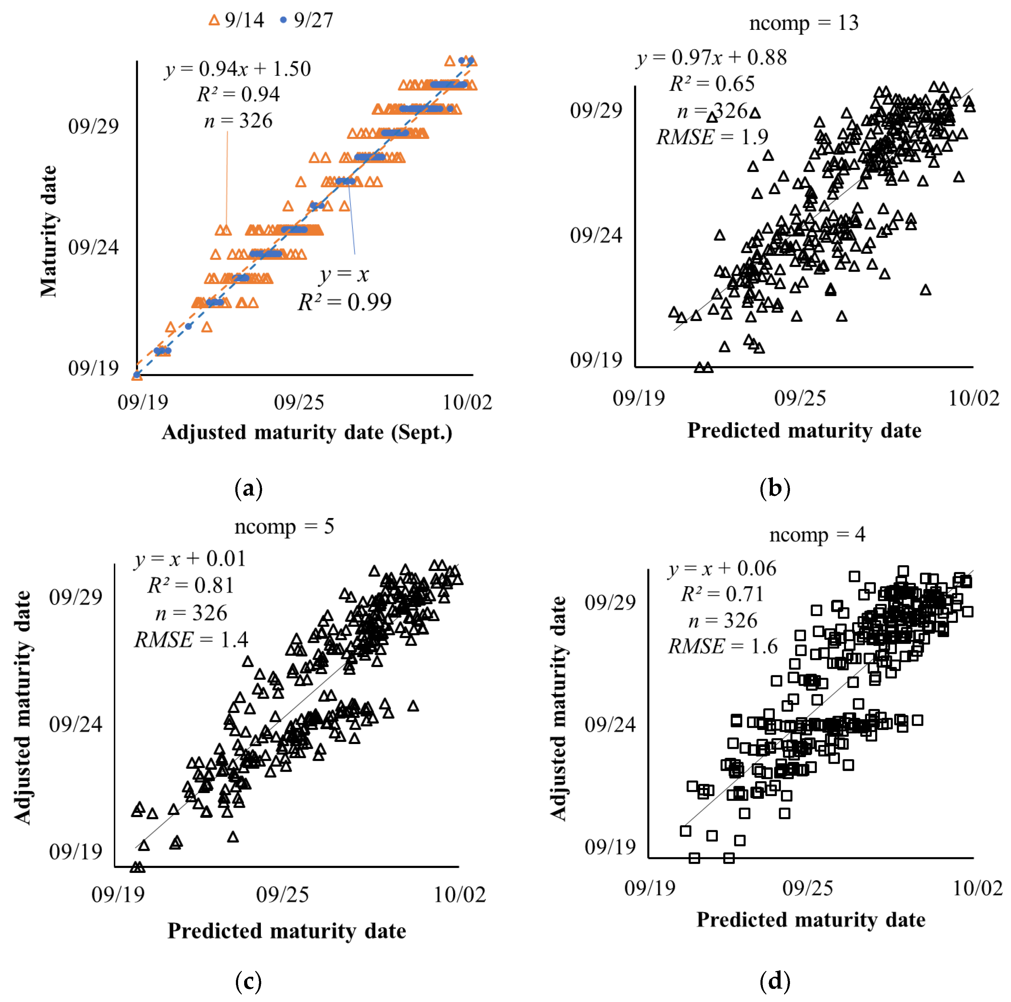
3.1. Estimation of Soybean Maturity Dates Using PLSR

The maturity dates estimated using the PLSR models with a 10-fold cross-validation on the three days are shown in Figure 3. Figure 3a illustrates the percent variance explained in maturity dates with the number of PLSR components. Variance in maturity dates can be explained up to 59%, 77% and 83% using image features on 27 August, 14 September and 27 September, respectively. Figure 3b shows the changes of RMSE with the number of PLSR components and the optimal number of components for each day was determined when the RMSE reaches the minimum on that day. The estimation using image features on 27 September had the lowest RMSE of 1.7 with five components followed by the one on 14 September (RMSE = 1.8) with 24 components and 27 August (RMSE = 2.7) with seven components. Thus, the optimal numbers of components for the PLSR model on the three days are 7, 24 and 5, respectively.
Figure 3c–e show the correlations between manual maturity dates and predicted maturity dates from PLSR models with the optimal numbers of components. When using image features of soybean lines in the middle of their maturity stage (R8, 27 September), there was the best agreement (R2 = 0.82) of predicted maturity dates and manual measurements.

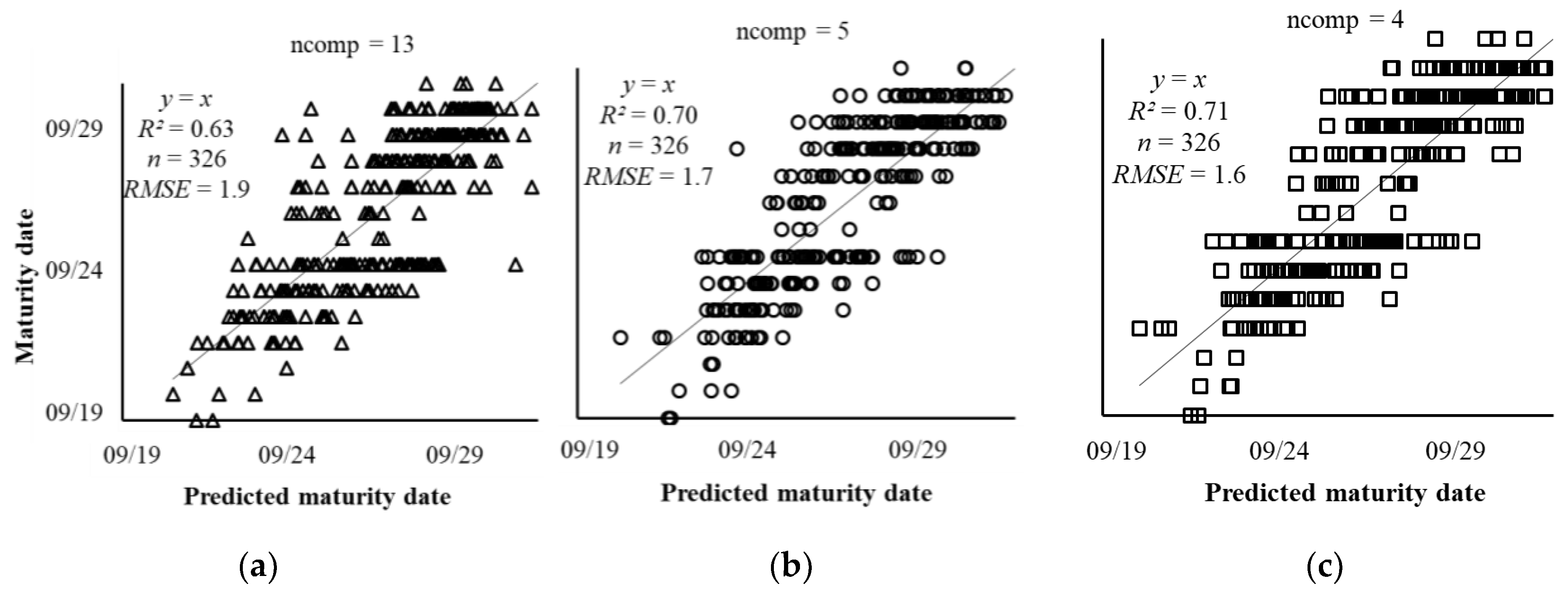
3.2. Model Parsimony

Figure 4 shows the VIP scores of 130 predictors of the PLSR models on the three days. There were 42, 56 and 73 predictors with VIP scores equal or greater than 1 in models on August 27, September 14 and September 27, respectively.
VIFs of these predictors were then calculated and those with VIFs less than 5 are shown in Table 2. Table 2 also shows the Pearson correlations between the maturity dates and the selected predictors (image features) from PLSR models on the three days. It can also be seen that there were few image features overlapping in the PLSR models for all the three days. The possible reason is that there were strong collinearities existing among all the 130 image features so that those with high Pearson correlations were not selected due to their high VIFs (>5).
In order to understand the different growth trends of soybean lines matured sequentially, the Pearson correlations between maturity dates and the selected image features in Table 2 were calculated and shown in Table 3. It can be seen that only three image features re_mean, CI_mean and IF_mean had significant linear relationships with the maturity dates on August 27, while the majority of image features on September 14 and September 27 are of significance.
Figure 5 shows the predicted maturity dates using three PLSR models with 20 selected images features and their changing rates. The estimations were performed using the same method mentioned in Section 2.5. The optimal numbers of components for the three PLSR models were 13, 5 and 4, respectively. Compared with Figure 3d,e, the PLSR models with changing rates in the selected image features taken between September 14 and September 27 improved the estimation accuracy (Figure 5b,c). The results indicate that there are certain patterns when images features of soybean lines with different maturity dates changed over time and these patterns could help to recognize the maturity dates. From Figure 5a,b, the model with the changing rates between September 14 and September 27 had higher estimation accuracy than the one with the changing rates between August 27 and September 14, showing the challenges in estimating maturity dates at early stages.

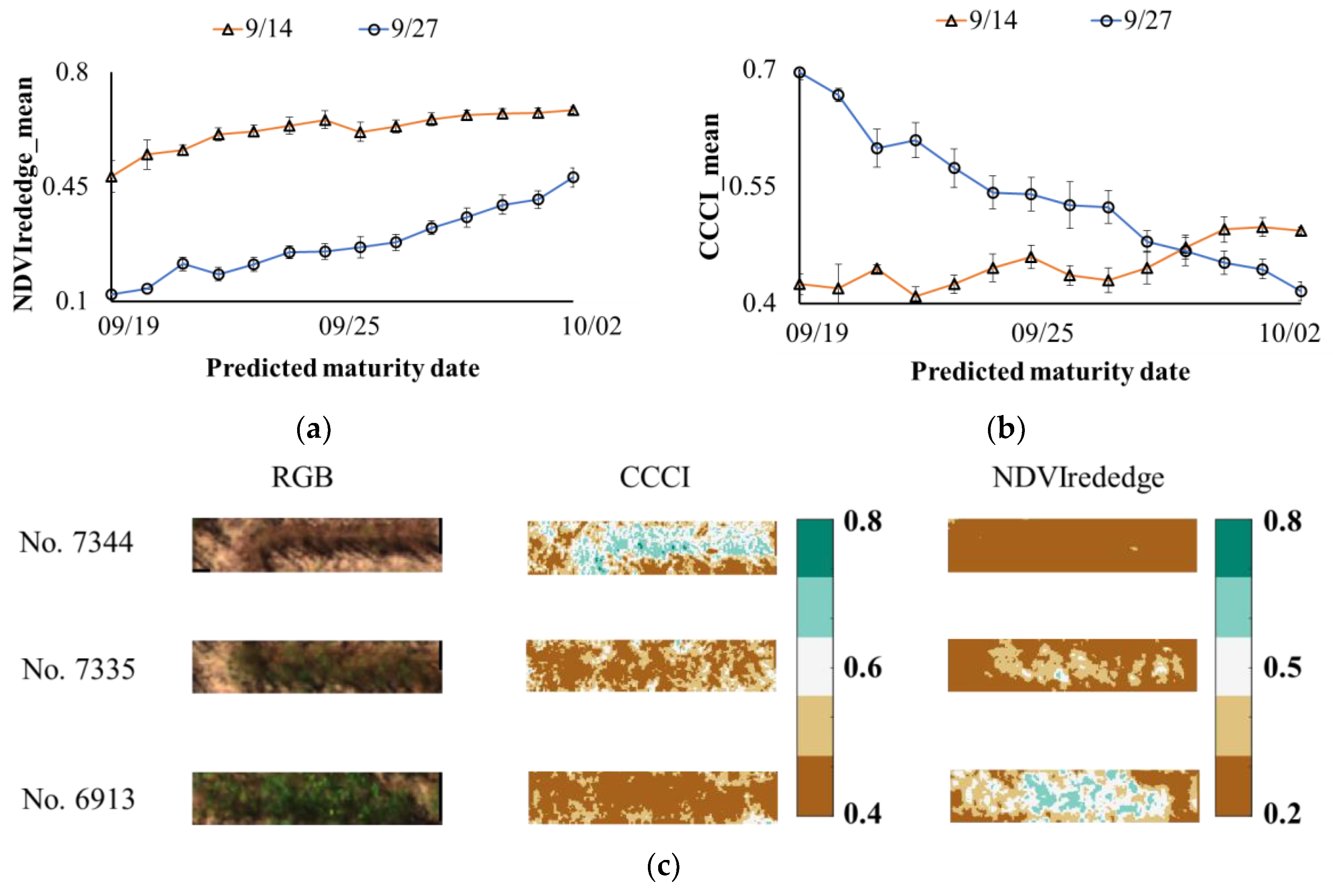
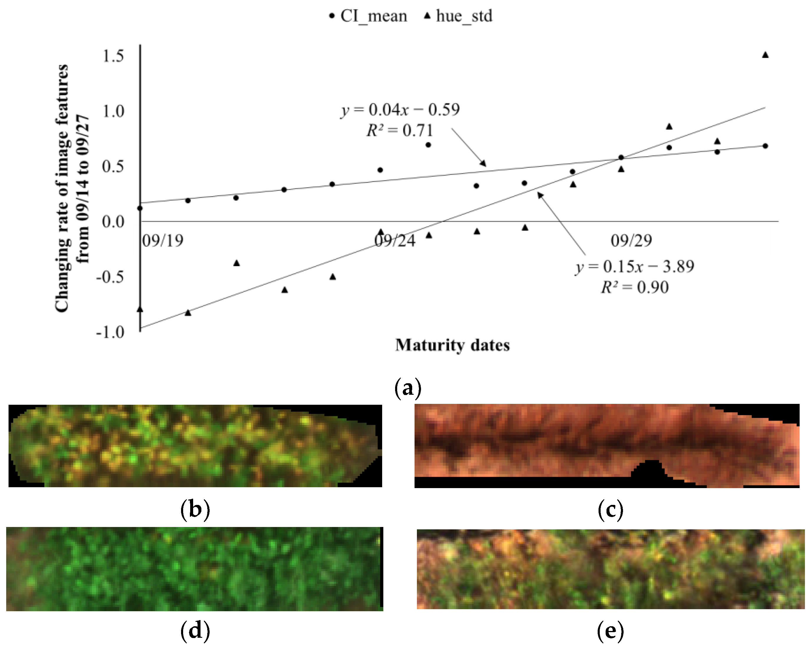
3.3. Adjusted Maturity Dates Based on the Variances in Image Features

Even though we can observe the monotonically increasing and decreasing trends in the selected image features against the maturity dates (Table 2), the variances in some days overlapped with other days (Figure 6a,b), especially when those soybean lines were close to their maturity, for example, the large variances in NDVIrededge_mean taken on 14 September were observed in those lines matured on 19 September and 20, and the large variances in CCCI_mean taken on 27 September were observed from 21 September to 27 September.
Figure 6c shows canopy images in these two vegetation indices of soybean lines (as shown in Figure 1) that were determined by visual ratings maturing at the same day (25 September). It can be seen that the dry stems had the highest CCCI values, while the green leaves had the lowest. When soybean lines had reached their R7 stages, the water content of the seeds are less than 50% and when they at R8 stages, the water content are less than 30% [10]. As an indicator of water stress suggested by Barnes Clarke [13], CCCI could represent various water content in soybean lines.
The NDVIrededge was first proposed by Gitelson and Merzlyak [26] and found that it was highly proportional to crop leaf chlorophyll content. It was calculated using the Red (668 nm) band with the Red Edge (717 nm) band and has shown a strong linear proxy (R2 = 0.94) of the green portion of the fraction of absorbed photosynthetically active radiation (fAPAR) that is sensitive to chlorophyll content in maize and soybean canopy [27]. It is consistent with our observation that the soybean line with more remaining leaves (No. 6913) had higher NDVIrededge values while the dry line (No. 7344) had very low values.
The maturity dates of soybean lines were adjusted based on the variances of NDVIrededge_mean and CCCI_mean taken on 14 September and 27 September. The relationships between maturity dates and the adjusted maturity dates were shown in Figure 7. The PLSR models were used to predict the maturity dates using the same method mentioned in Section 2.5 and the estimations are shown in Figure 7b–c.

4. Discussion and Future Work

4.1. Estimation of Soybean Maturity Dates at Different Growth Stages

The estimation of soybean maturity dates using PLSR with image features collected on different days in Figure 2 shows that the best agreement of predicted maturity dates and manual measurements was made by image features in the middle of their maturity stage, while the worst is by those collected when none of the soybean lines started maturing.
From Table 2, there was only one image feature (re_mean) had a significant linear relationship with the maturity dates on 27 August, while there were nine and five image features highly correlated (p-value < 0.05) with the maturity dates for 14 September and 27 September, respectively, indicating the challenge in estimating maturity date at early stage. We can also see that there were six common image features selected for PLSR models on 27 August and 14 September, and five of them had significant linear relationships on 14 September. These image features had the potential to be used as predictors, but they have not shown the trends at the early stage when mostly soybean lines remained green (Figure 1a).
Again, it can be seen from Table 3 that only three image features re_mean, CI_mean and IF_mean had significant linear relationships with the maturity dates on 27 August, while the majority of image features on 14 September and 27 September were of significance. It may indicate a higher accuracy in estimation of maturity date using data from later stages than early stages, as implied by the estimations from the PLSR models (Figure 3).

4.2. Selected Features for Parsimonious Models

For all the three days, five image features (CIrededge_mean, GDVI_std, GRVI_mean and BNDVI_mean) had positive linear relationships with the maturity dates, and four image features (S_mean, CVI_std, IF_std, CI_mean and IF_mean) were negatively related to the maturity dates, suggesting that these image features of all soybean lines kept increasing or decreasing from the beginning to the full maturity stage so that they can maintain consistent trends no matter which stage the image features were collected at. As shown in Figure 8a, for all the soybean lines, the changing rates in CI_mean were above 0 due to the increased CI_mean in all soybean lines from 14 September to 27 September. It was also observed that the changing rates in soybean lines matured later were greater than those in lines matured early, leading to a positive linear relationship between the changing rates in CI_mean and the maturity dates.
It should be noticed that the Pearson correlation coefficients of the other 11 image features in Table 3 had opposite signs for the three days, especially for the latter two days, such as re_mean, CCCI_std, CI_std, NormG_std, hue_std and GRNDVI_std. The reason may be that for the soybean lines matured at different days, there were different changing rates in such features. From Figure 8a, the changing rates in hue_std were significantly less than 0 for lines matured before 24 September, indicating the hue_std of these lines decreased from 14 September to 27 September. For lines matured during 24 September to 27 September, the changing rates in hue_std were very close to 0, suggesting that the hue_std in these lines barely changed between two data collection days. For lines matured after 27 September, the changing rates were significantly greater than 0, showing that there were increased hue_std in these lines. It might be due to the gradually occurrence of yellow leaves when the soybean lines were closed to their maturity (Figure 8b), leading to high variances in hue, while those lines matured late still had more green leaves (Figure 8c). When hue was calculated on 27 September, matured soybean lines had more dry leaves than fresh leaves (Figure 8d), leading to low variances, while the late-matured lines were stepping into their R8 stages (Figure 8e), resulting in high variances. Similar situations could happen in other image features with opposite linear relationships for the latter two days.

4.3. Adjusted Maturity Dates

In Figure 7a, the adjusted maturity dates for both image collection days were extended around their observed maturity dates, which might help to tolerate the variances of canopy green leaves as well as errors from subjective judgments and estimations of breeders. By using the adjusted maturity dates as ground reference, the RMSE dropped from 1.7 to 1.4 and the R2 increased to 0.81 using the selected images features taken on 14 September and their changing rates between 14 September and 27 September, while nearly no changes occurred on the other two models. It might be because these two image features captured more variances on 14 September than those on 27 September.
By personal communication with breeders, RMSE within 1.5 days can be considered as a tolerable error in soybean breeding programs. Compared to previous studies, our study shows improvements on predicting the exact maturity dates instead of the classification between mature and immature lines [9], as well as making a more practical prediction (with an acceptable accuracy) for breeding programs [14]. Therefore, it can be concluded that it is a promising method to predict soybean maturity dates using UAV-based multispectral image features by screening the soybean lines once at the beginning of maturity stage to quantify the variances in canopies, and another one at the middle of the full maturity stage to track the canopy changes.
As the adjusted maturity dates are first proposed in this study to tolerate the variances of canopy green leaves for the purpose of predicting soybean maturity dates using canopy image features, the maturity dates were adjusted based on the variances in two image features with known matured dates in a single environment. In soybean breeding programs, RMs of a variety from around 40–50 environments are required to assign a MG to the variety. Therefore, the variances need to be quantified in future studies by repeating the experiments in multiple environments and documenting the image features.
Errors could be introduced by many factors regarding image features. Due to the limited field of view of the multispectral camera, the 3.64 ha field was fully screened by three flight missions during the time period of more than 2 h, including taking off and landing the UAV, changing batteries and calibration. Light changes during image collection were conjunctions of many factors, such as the changing relative position between sun and drone, various light diffusions caused by the thin cloud in the sky and the random exiting thick clouds, which resulted in cloud shadows in the images (not observed in this study) [28]. Another inevitable source of variation is some blurred portions of orthomosaic caused by image stitching. At the later stage of soybean growth, soybean lines with big canopies can touch and overlap with their neighbors and leaves on immature lines are yellow or in the transition to yellow, which were hard to be distinguished with soil. Under this scenario, blurs and even undetectable misalignments of breeding lines might occur in the orthomosaic.

4.4. Future Work

In future studies, the variances in image features to adjust the maturity dates need to be quantified and derived by repeating the experiments in multiple environments and documenting image features. There was also two major issues expected to be addressed to reduce errors introduced during the image collection and processing pipeline. First, as an image pixel value is the reflectance of incoming solar irradiance, the variation in light conditions could introduce variations to image-derived features. The relationship between light changes during UAV flight missions and camera responses (reflectance) should be further explored and flight dynamics (drone pose, sun’s position, light diffusion, clouds, etc.) need to be better integrated to describe the light changes. Second, variations are inevitably introduced when images are stitched based on features recognition. Instead of localizing individual breeding lines from an orthomosaic, efforts have to be made to investigate the potential of direct georeferencing that geometric position of a breeding line is the conjunction of the relative position of the line in an image and the UAV position where the image was taken. With direct georeferencing, flight attitude and speed can be liberated from high image overlaps (≥ 70% for creating orthomosaic images) so that the time issue and light variation can be moderated consequently.

5. Conclusions

The potential of predicting maturity dates of soybean breeding lines using UAV-based multispectral imagery was investigated in this paper. Maturity dates of 326 soybean breeding lines were taken using visual ratings from the beginning maturity stage (R7) to full maturity stage (R8), and the aerial multispectral images were also taken during this period on 27 August, 14 September and 27 September. One hundred and thirty features were extracted from the five-band multispectral images. The maturity dates of soybean lines were predicted and evaluated using PLSR models with 10-fold cross-validation. The results showed that the estimations at later stages had a better accuracy than those at earlier stages. Twenty image features with importance were then selected to simplify the PLSR models. The changing rates in image features between each of the two collection days were calculated. The estimation accuracy was improved by the simplified PLSR models with the selected image features and their changing rates. The adjusted maturity dates were proposed to tolerate the variances of canopy green leaves and calculated based on the variances in NDVIrededge_mean and CCCI_mean. The best prediction (R2 = 0.81, RMSE = 1.4 days) was made by the PLSR model using selected images features taken on 14 September and their changing rates between 14 September and 27 September as predictors and the adjusted maturity dates as responses with five components. This study outperformed other similar studies in terms of prediction accuracy and practical usefulness. Another contribution of this paper is that based on our observations from canopy images, the adjusted maturity dates were proposed to tolerate the variances of canopy green leaves as well as errors from subjective judgments and estimations of breeders.

Author Contributions

Conceptualization, A.S. and J.Z. (Jianfeng Zhou); methodology, J.Z. (Jing Zhou); formal analysis, J.Z. (Jing Zhou); investigation, J.Z. (Jing Zhou), D.Y. and C.N.V.; resources, A.S.; writing—original draft preparation, J.Z. (Jing Zhou); writing—review and editing, A.S., D.Y., C.N.V. and J.Z. (Jianfeng Zhou); supervision, J.Z. (Jianfeng Zhou)

Funding

This research received no external funding.

Acknowledgments

We would like to thank Joshua Dakota and other colleagues in Bay Farm Research Facility of the Missouri Soybean Association for their kindly help in plant material preparation and colleagues in Greenley Research Center at the University of Missouri in field operations and management. We also would like to thank our colleague Dandan Fu from Huazhong Agricultural University, China for her kind help in conducting experiments.

Conflicts of Interest

The authors declare no conflict of interest.

Appendix A

Table A1. Vegetation indices.
No.Index NameDescriptionsFormula
1NDVINormalized difference VI* n i r r e d n i r + r e d
2ATSAVIAdjusted transformed soil-adjusted VI 1.22 × nir 1.22 × red 0.03 1.22 n i r + r e d 0.0366 + 0.08 × ( 1 + a 2 )
3ARVI2 Atmospherically Resistant VI 2 0.18 + 0.17 × n i r r e d n i r + r e d
4BWDRVI Blue-wide dynamic range VI 0.1 × n i r r e d 0.1 × n i r + r e d
5CCCI Canopy Chlorophyll Content Index n i r r e n i r + r e N D V I
6CIgreen Chlorophyll Index Green n i r g r e e n 1
7CIrededgeChlorophyll Index RedEdge n i r r e 1
8CVIChlorophyll VI n i r × r e d g r e e n 2
9CIColoration Index r e d b l u e r e d
10CTVICorrected Transformed VI N D V I + 0.5 | N D V I + 0.5 | × | N D V I + 0.5 |
11GDVIGreen Difference VI n i r g r e e n
12EVIEnhanced VI 2.5 × n i r r e d n i r + 6 × r e d 7.5 × b l u e + 1
13EVI2 Enhanced VI 2 2.4 × n i r r e d n i r + r e d + 1
14EVI22Enhanced VI 2-2 2.5 × n i r r e d n i r + 2.4 × r e d + 1
15GEMIGlobal Environment Monitoring Index a =   2 × ( n i r 2 r e d 2 ) + 1.5 × n i r + 0.5 × r e d n i r + r e d + 0.5
G E M I = a × ( 1 0.25 × a ) r e d 0.125 1 r e d
16GARIGreen atmospherically resistant VI n i r ( g r e e n ( b l u e r e d ) ) n i r + ( g r e e n + ( b l u e r e d ) )
17GLIGreen leaf index 2 × g r e e n r e d b l u e 2 × g r e e n + r e d + b l u e
18GBNDVIGreen-Blue NDVI n i r ( g r e e n + b l u e ) n i r + ( g r e e n + b l u e )
19GRNDVIGreen-Red NDVI n i r ( g r e e n + r e d ) n i r + ( g r e e n + r e d )
20HHue tan 1 ( 2 × r e d g r e e n b l u e 30.5 × ( g r e e n b l u e ) )
21IPVIInfrared percentage VI n i r 2 × ( n i r + r e d ) × N D V I
22IIntensity r e d + g r e e n + b l u e 30.5
23LogRLog Ratio l o g ( n i r r e d )
24MSAVIModified Soil Adjusted VI 1 2 × ( 2 × n i r + 1 ( 2 × n i r + 1 ) 2 8 × ( n i r r e d ) )
25NormGNorm Green g r e e n n i r + r e d + g r e e n
26NormNIRNorm NIR n i r n i r + r e d + g r e e n
27NormR Norm Red r e d n i r + r e d + g r e e n
28NGRDINormalized green red difference index g r e e n r e d g r e e n + r e d
29BNDVIBlue-normalized difference VI n i r b l u e n i r + b l u e
30GNDVIGreen NDVI n i r g r e e n n i r + g r e e n
31NDRENormalized Difference Red-Edge n i r r e n i r + r e .
32RIRedness Index r e d g r e e n r e d + g r e e n
33NDVIrededgeNormalized Difference Rededge/Red r e r e d r e + r e d
34PNDVIPan NDVI n i r ( g r e e n + r e d + b l u e ) n i r + ( g r e e n + r e d + b l u e )
35RBNDVIRed-Blue NDVI n i r ( r e d + b l u e ) n i r + ( r e d + b l u e )
36IFShape Index 2 × r e d g r e e n b l u e g r e e n b l u e
37GRVIGreen Ratio VI n i r g r e e n
38DVIDifference VI n i r r e d
39RRI1RedEdge Ratio Index 1 n i r r e
40IOIron Oxide r e d b l u e
41RGRRed–Green Ratio r e d g r e e n
42SRRedNIRRed/NIR Ratio VI r e d n i r
43RRI2Rededge/Red RedEdge Ratio Index 2 r e r e d
44SQRTIRR SQRT(IR/R) n i r r e d
45TNDVITransformed NDVI n i r r e d n i r + r e d + 0.5
46TGITriangular greenness index 0.5 × ( 0.19 × ( r e d g r e e n ) 0.12 × ( r e d b l u e ) )
47WDRVIWide Dynamic Range VI 0.1 × n i r r e d 0.1 × n i r + r e d
48MSRModified Simple Ratio r e d n i r r e d + 1
49MTVI2Modified Triangular VI 1.5 × ( 1.2 × ( n i r g r e e n ) 2.5 × ( r e d g r e e n ) ) ( 3 n i r ) 2 6 × n i r + 5 × r e d 0.5
50RDVIRenormalized Difference VI n i r r e d n i r + r e d
51IRGRed Green Ratio Index r e d g r e e n
52OSAVIOptimized Soil Adjusted VI n i r r e d n i r + r e d + 0.16
53SRNDVISimple Ratio × Normalized Difference Vegetation Index n i r 2 r e d n i r + r e d 2
54SARVI2Soil and Atmospherically Resistant Vegetation Index 2 2.5 × n i r r e d 1 + n i r + 6 × r e d 7.5 × b l u e
*VI: Vegetation index.

References

  1. Hincks, J.; The World Is Headed for a Food Security Crisis. Here’s How We Can Avert It. 2018. Available online: https://www.un.org/development/desa/en/news/population/world-population-prospects-2017.html (accessed on 15 February 2019).
  2. Breene, K. Food Security and Why It Matters. 2018. Available online: https://www.weforum.org/agenda/2016/01/food-security-and-why-it-matters/ (accessed on 15 February 2019).
  3. Sun, M. Efficiency Study of Testing and Selection in Progeny-Row Yield Trials and Multiple-Environment Yield Trials in Soybean Breeding. Ph.D. Thesis, Iowa State University, Ames, IA, USA, 2014. [Google Scholar]
  4. Breseghello, F.; Coelho, A.S.G. Traditional and Modern Plant Breeding Methods with Examples in Rice (Oryza sativa L.). J. Agric. Food Chem. 2013, 61, 8277–8286. [Google Scholar] [CrossRef] [PubMed]
  5. Staton, M. What Is the Relationship between Soybean Maturity Group and Yield; Michigan State University Extension: East Lansing, MI, USA, 2017. [Google Scholar]
  6. Mourtzinis, S.; Conley, S.P. Delineating Soybean Maturity Groups across the United States. Agron. J. 2017, 109, 1397. [Google Scholar] [CrossRef]
  7. Fehr, W. Principles of Cultivar Development: Theory and Technique; Macmillan Publishing Company: London, UK, 1991. [Google Scholar]
  8. Masuka, B.; Atlin, G.N.; Olsen, M.; Magorokosho, C.; Labuschagne, M.; Crossa, J.; Bänziger, M.; Pixley, K.V.; Vivek, B.S.; von Biljon, A.; et al. Gains in Maize Genetic Improvement in Eastern and Southern Africa: I. CIMMYT Hybrid Breeding Pipeline. Crop Sci. 2017, 57, 168–179. [Google Scholar] [CrossRef] [Green Version]
  9. Yu, N.; Li, L.; Schmitz, N.; Tian, L.F.; Greenberg, J.A.; Diers, B.W. Development of methods to improve soybean yield estimation and predict plant maturity with an unmanned aerial vehicle based platform. Remote Sens. Environ. 2016, 187, 91–101. [Google Scholar] [CrossRef]
  10. Fehr, W.R.; Caviness, C.E.; Burmood, D.T.; Pennington, J.S. Stage of Development Descriptions for Soybeans, Glycine max (L.) Merrill1. Crop Sci. 1971, 11, 929. [Google Scholar] [CrossRef]
  11. Peske, S.T.; Höfs, A.; Hamer, E. Seed moisture range in a soybean plant. Rev. Bras. Sement. 2004, 26, 120–124. [Google Scholar] [CrossRef]
  12. Rundquist, D.C.; Gitelson, A.A.; Viña, A.; Arkebauer, T.J.; Keydan, G.; Leavitt, B. Remote estimation of leaf area index and green leaf biomass in maize canopies. Geophys. Res. Lett. 2003, 30. [Google Scholar] [CrossRef] [Green Version]
  13. Barnes, E.; Clarke, T.R.; Richards, S.E.; Colaizzi, P.D.; Haberland, J.; Kostrzewski, M.; Waller, P.; Choi, C.; Riley, E.; Thompson, T. Coincident detection of crop water stress, nitrogen status and canopy density using ground based multispectral data. In Proceedings of the Fifth International Conference on Precision Agriculture, Bloomington, MN, USA, 16–19 July 2000. [Google Scholar]
  14. Christenson, B.S.; Schapaugh, W.T.; An, N.; Price, K.P.; Prasad, V.; Fritz, A.K. Predicting Soybean Relative Maturity and Seed Yield Using Canopy Reflectance. Crop. Sci. 2016, 56, 625. [Google Scholar] [CrossRef]
  15. MicaSense. Use of Calibrated Reflectance Panels for RedEdge Data. 2017. Available online: https://support.micasense.com/hc/en-us/articles/115000765514-Use-of-Calibrated-Reflectance-Panels-For-RedEdge-Data (accessed on 20 April 2019).
  16. MicaSense. How to Process RedEdge Data in Pix4D. 2018. Available online: https://support.micasense.com/hc/en-us/articles/115000831714-How-to-Process-RedEdge-Data-in-Pix4D (accessed on 20 April 2019).
  17. Yang, C.; Everitt, J.H.; Bradford, J.M.; Murden, D. Airborne Hyperspectral Imagery and Yield Monitor Data for Mapping Cotton Yield Variability. Precis. Agric. 2004, 5, 445–461. [Google Scholar] [CrossRef]
  18. Hancock, D.W.; Dougherty, C.T. Relationships between Blue- and Red-based Vegetation Indices and Leaf Area and Yield of Alfalfa. Crop Sci. 2007, 47, 2547–2556. [Google Scholar] [CrossRef]
  19. Agapiou, A.; Hadjimitsis, D.G.; Alexakis, D.D. Evaluation of Broadband and Narrowband Vegetation Indices for the Identification of Archaeological Crop Marks. Remote Sens. 2012, 4, 3892–3919. [Google Scholar] [CrossRef] [Green Version]
  20. Henrich, V.; Götze, C.; Jung, A.; Sandow, C. Development of an Online indices-database: Motivation, concept and implementation. In Proceedings of the 6th EARSeL Imaging Spectroscopy SIG Workshop Innovative Tool for Scientific and Commercial Environment Applications, Tel Aviv, Israel, 16–19 March 2009. [Google Scholar]
  21. Ishtiaq, K.S.; Abdul-Aziz, O.I. Relative Linkages of Canopy-Level CO2 Fluxes with the Climatic and Environmental Variables for US Deciduous Forests. Environ. Manag. 2015, 55, 943–960. [Google Scholar] [CrossRef]
  22. Eigenvector Research. Vip. 2018. Available online: http://wiki.eigenvector.com/index.php?title=Vip (accessed on 15 February 2019).
  23. MathWorks Support Team. How to Calculate the Variable Importance in Projection from Outputs of PLSREGRESS. Available online: https://www.mathworks.com/matlabcentral/answers/443239-how-to-calculate-the-variable-importance-in-projection-from-outputs-of-plsregress (accessed on 15 February 2019).
  24. James, G.; Witten, D.; Hastie, T.; Tibshirani, R. An Introduction to Statistical Learning; Springer: Berlin/Heidelberg, Germany, 2013; Volume 112. [Google Scholar]
  25. Chen, D.; Neumann, K.; Friedel, S.; Kilian, B.; Chen, M.; Altmann, T.; Klukas, C. Dissecting the phenotypic components of crop plant growth and drought responses based on high-throughput image analysis. Plant Cell 2014, 26, 4636–4655. [Google Scholar] [CrossRef] [PubMed]
  26. Gitelson, A.; Merzlyak, M.N. Spectral Reflectance Changes Associated with Autumn Senescence of Aesculus hippocastanum L. and Acer platanoides L. Leaves. Spectral Features and Relation to Chlorophyll. Estim. J. Plant Physiol. 1994, 143, 286–292. [Google Scholar] [CrossRef]
  27. Viña, A.; Gitelson, A.A. New developments in the remote estimation of the fraction of absorbed photosynthetically active radiation in crops. Geophys. Res. Lett. 2005, 32. [Google Scholar] [CrossRef] [Green Version]
  28. MicaSense. DLS Sensor Basic Usage. 2017. Available online: https://micasense.github.io/imageprocessing/MicaSense%20Image%20Processing%20Tutorial%203.html (accessed on 20 April 2019).
Figure 1. Orthomosaic images of part of the soybean field. (a,c) are the colorful images with the red (r), green (g) and blue (b) channels of images acquired on 27 August and 27 September. (b) The grayscale image of blue normalized difference vegetation index (BNDVI) derived from images taken on 27 August and (d) the grayscale image of blue-wide dynamic range vegetation index (BWDRVI) derived from images taken on 27 September. (e,f) are histograms of image pixel values in the two red rectangles.
Remotesensing 11 02075 g001
Figure 2. Illustration of variations in canopy images of the soybean lines matured on 25 September. Images were generated using r, g and b bands from the multispectral camera. Breeding line no. from left to right is: 7344, 7335 and 6913.
Remotesensing 11 02075 g002
Figure 3. Estimation of maturity dates using partial least square regression (PLSR). (a) Percent of variance explained in the maturity dates as a function of the number of components in the PLSR model. (b) Mean square error in the maturity dates as a function of the number of components. (c)–€ The correlations between manual maturity dates and predicted maturity dates using images features taken on 27 August, 14 September and 27 September, respectively. ncomp: The optimal number of components.
Remotesensing 11 02075 g003
Figure 4. Variable importance in projection (VIP) scores of 130 predictors of the PLSR models on the three days.
Remotesensing 11 02075 g004
Figure 5. Estimation of maturity dates using PLSR models with selected images features and the changing rates. (a) The correlations between manual maturity dates and predicted maturity dates using the selected images features taken on 14 September and their changing rates between 27 August and 14 September. (b) The correlations using the selected images features taken on 14 September and their changing rates between 14 September and 27 September. (c) The correlations using the selected images features taken on 27 September and their changing rates between 14 September and 27 September.
Remotesensing 11 02075 g005
Figure 6. Vegetation indices CCCI and NDVIrededge. (a)–(b) The relationships between maturity dates and NDVIrededge_mean and CCCI_mean collected on 14 September and 27 September. (c) Canopy images of the soybean lines matured on 25 September in RGB, CCCI and NDVIrededge.
Remotesensing 11 02075 g006
Figure 7. Adjusted maturity dates. (a) The relationship between maturity dates and the adjusted maturity dates based on the variances of NDVIrededge_mean and CCCI_mean taken on 14 September and 27 September. (b) The correlations between adjusted maturity dates and predicted maturity dates using the selected image features taken on 14 September and their changing rates between 27 August and 14 September. (c) The correlations using the selected image features taken on 14 September and their changing rates between 14 September and 27 September. (d) The correlations using the selected image features taken on 27 September and their changing rates between 14 September and 27 September.
Remotesensing 11 02075 g007
Figure 8. The changing rates in CI_mean and hue_std from 14 September and 27 September. (a) The changing rates in CI_mean and hue_std. (b,d) are RGB images of a line matured on 19 September, and they were taken on 14 September and 27 September, respectively. (c,e) are RGB images of a line matured on 1 October, and they were taken on 14 September and 27 September, respectively.
Remotesensing 11 02075 g008
Table 1. Wavelength information of the camera and the reflectance in each band of the calibration reflectance panel (CRP).
Band NameCenter Wavelength (nm)Bandwidth * (nm)Reflectance (%)
Blue (b)4752049.2
Green (g)5602049.3
Red (r)6681049.1
Red edge (re)7171048.7
Near-infrared (nir)8404049.0
* Bandwidth is defined as the full width at half maximum (FWHM).
Table 2. Pearson correlations between the predictors with VIP scores ≥ 1 and variance inflation factors (VIFs) < 5 and maturity dates on the three days.
Image FeaturesAugust 27September 14September 27
re_mean–0.596 *
S_mean–0.501–0.697 **
CCCI_std–0.487–0.930 ***
Cirededge_mean0.5040.368
CVI_std–0.389
CI_std0.184–0.662 **
GDVI_std0.1770.861 ***
H_mean †0.102
NormG_std0.413–0.831 ***
IF_std–0.170
RRI2_std–0.239–0.227
CI_mean–0.935 ***
H_std–0.915 ***
GRVI_mean0.922 ***
MTVI2_std0.795 ***
hue_std ‡0.959 ***
GEMI_mean0.977 ***
GRNDVI_std0.959 ***
BNDVI_mean0.934 ***
IF_mean–0.991 ***
*, ** and *** indicate the significance at p = 0.05, 0.01 and 0.001 levels, respectively. † and ‡ represent the feature hue in HSV color space but was calculated using different methods. † uses the equation in Appendix A Table A1. ‡ is converted from the RGB image using the ‘rgb2hsv’ function in MATLAB.
Table 3. Pearson correlations between maturity dates and the means of image features at each maturity dates on the three days.
Image FeaturesAugust 27September 14September 27
re_mean–0.596 *–0.4140.890 ***
S_mean–0.501–0.697 **–0.830 ***
CCCI_std–0.487–0.930 ***0.605 *
Cirededge_mean0.5040.928 ***0.368
CVI_std–0.389–0.718 **–0.552 *
CI_std0.184–0.662 **0.931 ***
GDVI_std0.1770.861 ***0.845 ***
H_mean0.102–0.830 ***–0.409
NormG_std0.413–0.831 ***0.916 ***
IF_std–0.170–0.921 ***–0.585 *
RRI2_std–0.239–0.2270.981 ***
CI_mean–0.595 *–0.935 ***–0.886 ***
H_std–0.490–0.915 ***0.268
GRVI_mean0.4970.922 ***0.499
MTVI2_std–0.0350.795 ***0.989 ***
hue_std–0.413–0.931 ***0.959 ***
GEMI_mean–0.0040.857 ***0.977 ***
GRNDVI_std0.242–0.889 ***0.959 ***
BNDVI_mean0.3560.879 ***0.934 ***
IF_mean–0.544 *–0.879 ***–0.991 ***
*, ** and *** indicate the significance at p = 0.05, 0.01 and 0.001 levels, respectively.

