Developing a New Machine-Learning Algorithm for Estimating Chlorophyll-a Concentration in Optically Complex Waters: A Case Study for High Northern Latitude Waters by Using Sentinel 3 OLCI


Abstract
1. Introduction
- Introduce a unified Chl-a retrieval algorithm to monitor Chl-a concentration in complex high northern latitude waters, such as inland, coastal waters, the Marginal Ice Zone (MIZ), and for open Arctic oceans.
- Design the model specifically to S3 OLCI so that the advantageous spectral, spatial and temporal resolutions of the instrument can be used for monitoring these complex high northern latitude waters.
- Provide a tool to assess uncertainties in the retrieval of the Level 2 (L2) radiometric data, i.e., the Remote sensing reflectance (Rrs), which is the input to many of the Ocean Color algorithms, including the model introduced here.
2. Materials and Methods
2.1. Data
2.1.1. Training Data for Model Optimization
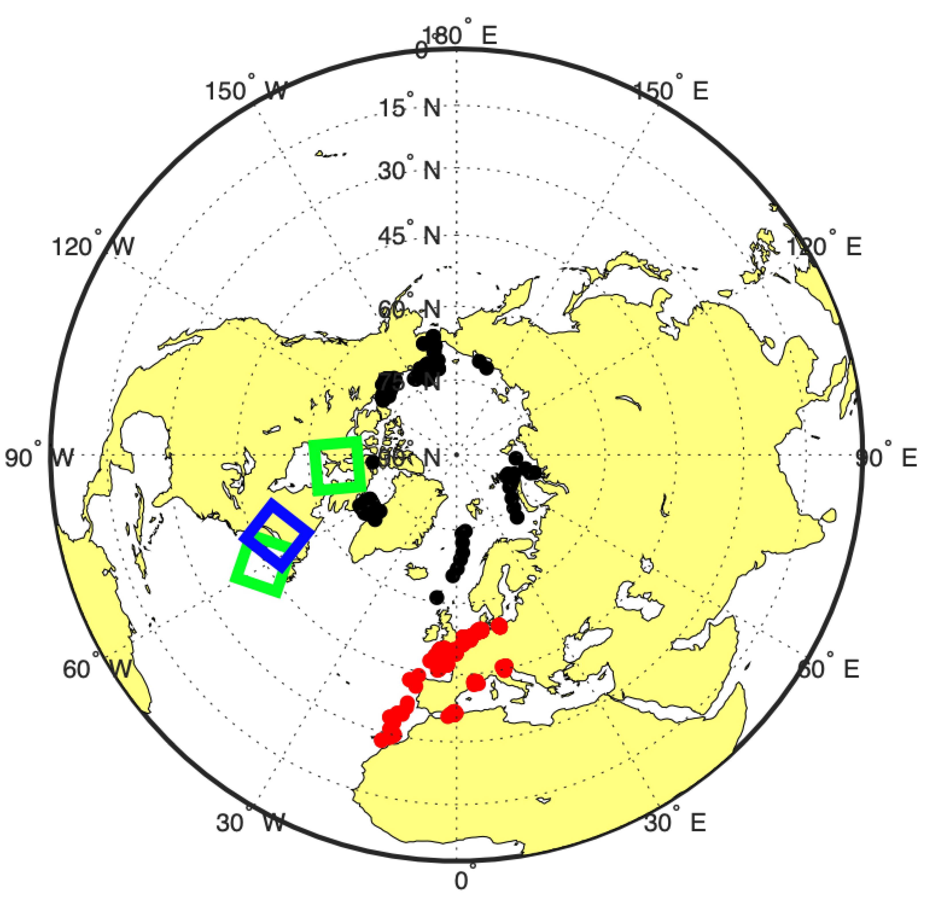
The Arctic Data
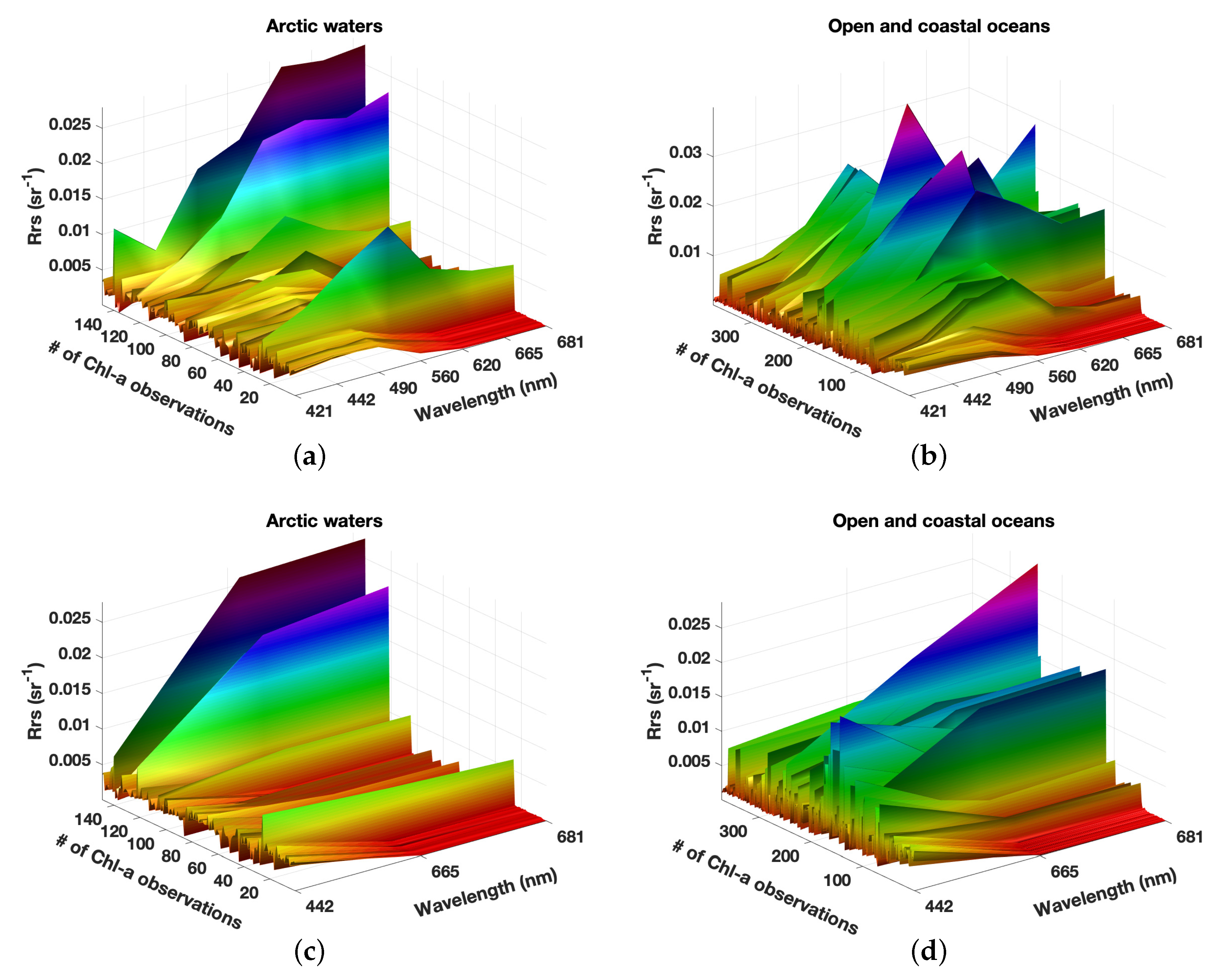
Rrs Measurements
The COASTlOOC Data
The Merged Global Data
Total Chl-a Measurements
2.1.2. Data for Prediction with the Trained ML GPR Balaton Model
2.2. Methodology
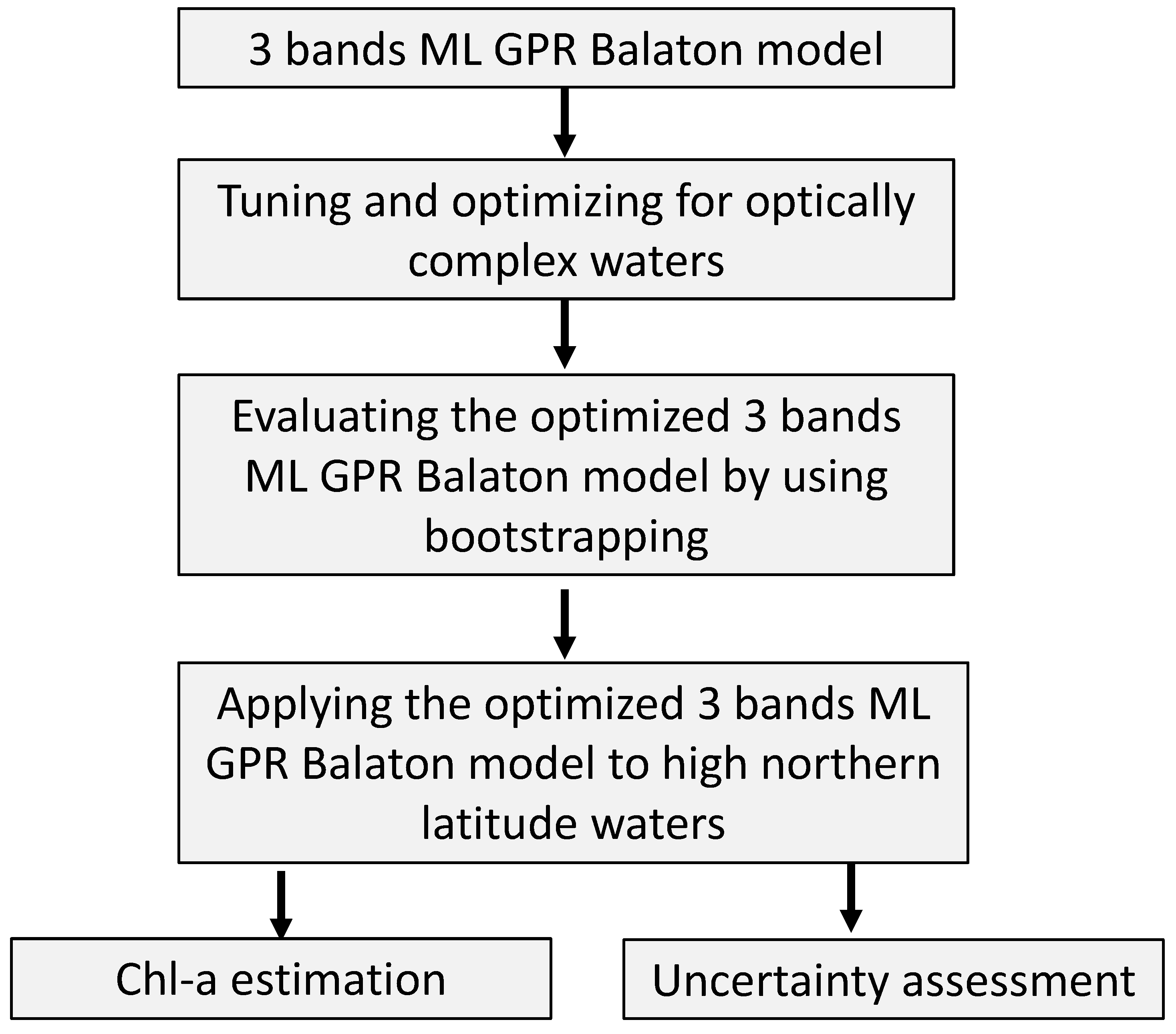
2.2.1. The ML GPR Balaton Model
2.2.2. Interpretation of the ML GPR Balaton Model
2.2.3. Description of the Analysis
3. Results
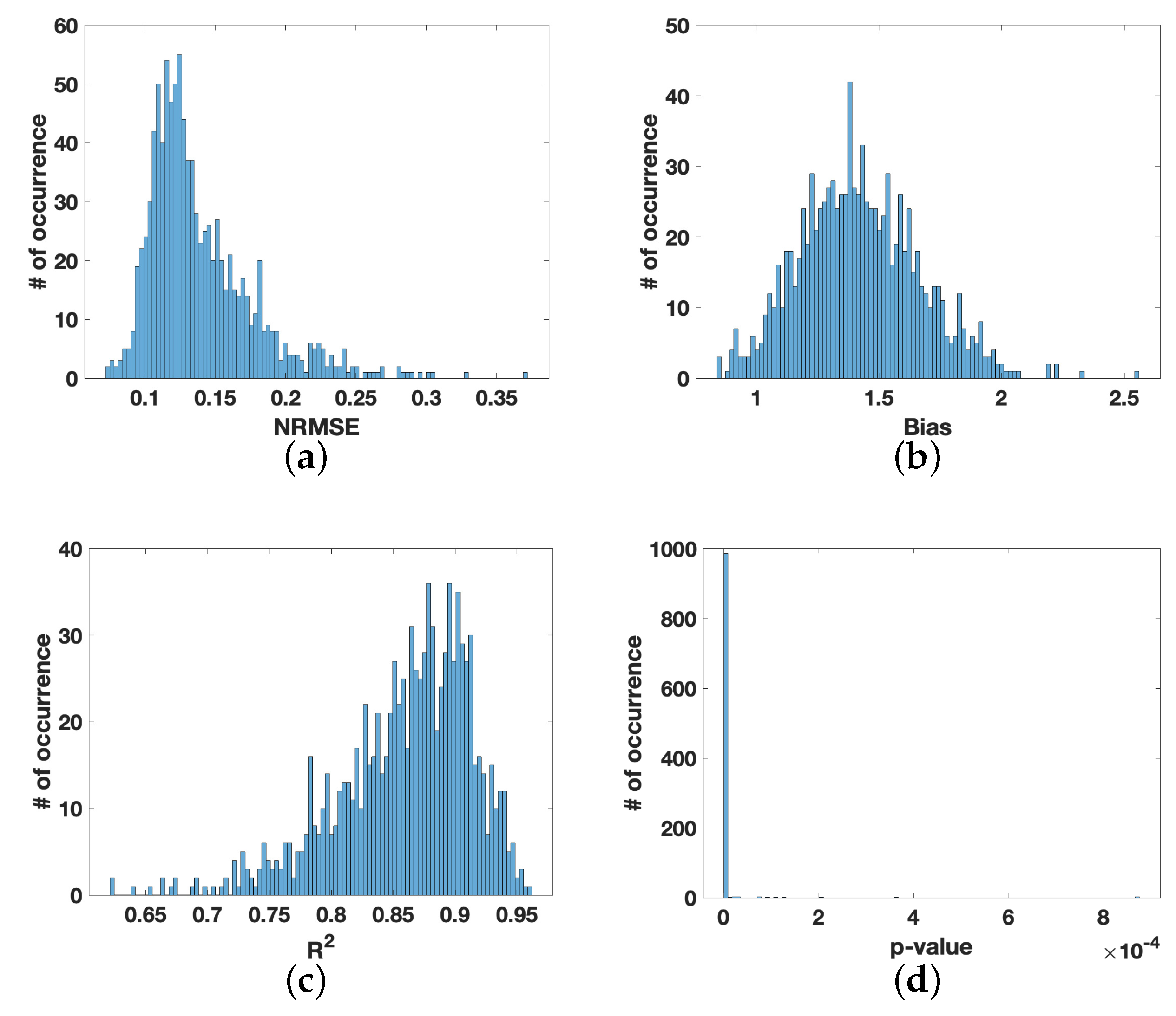
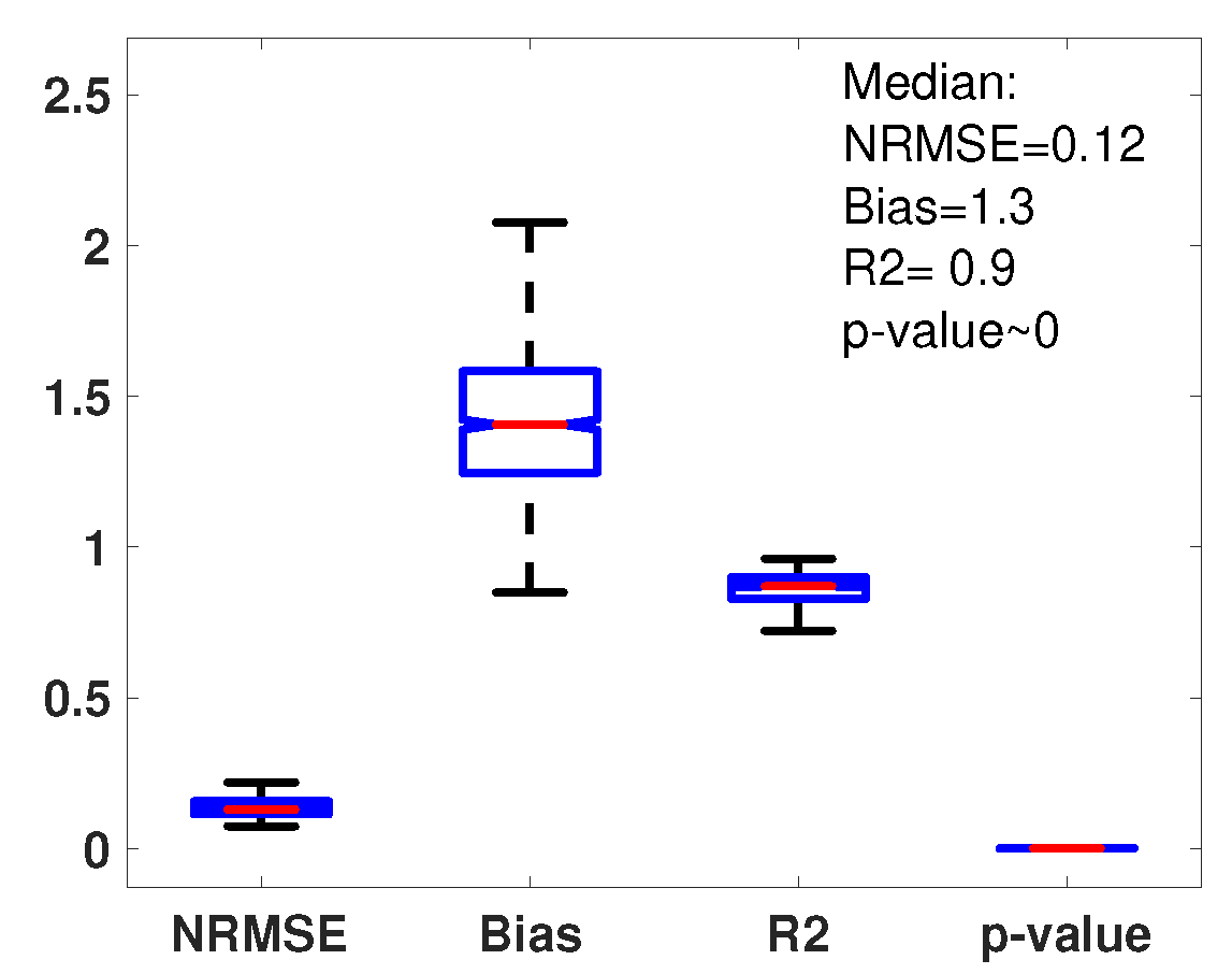
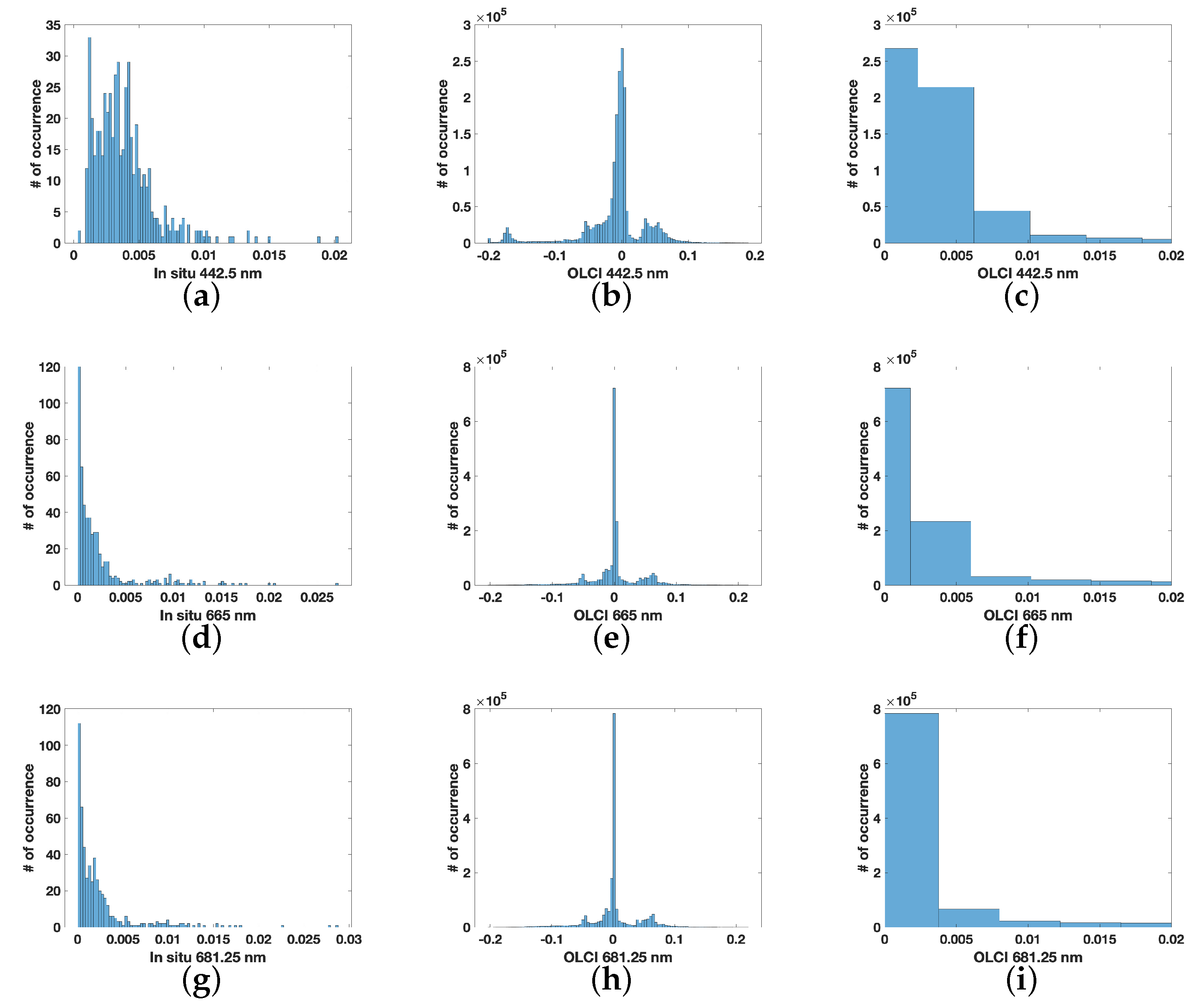
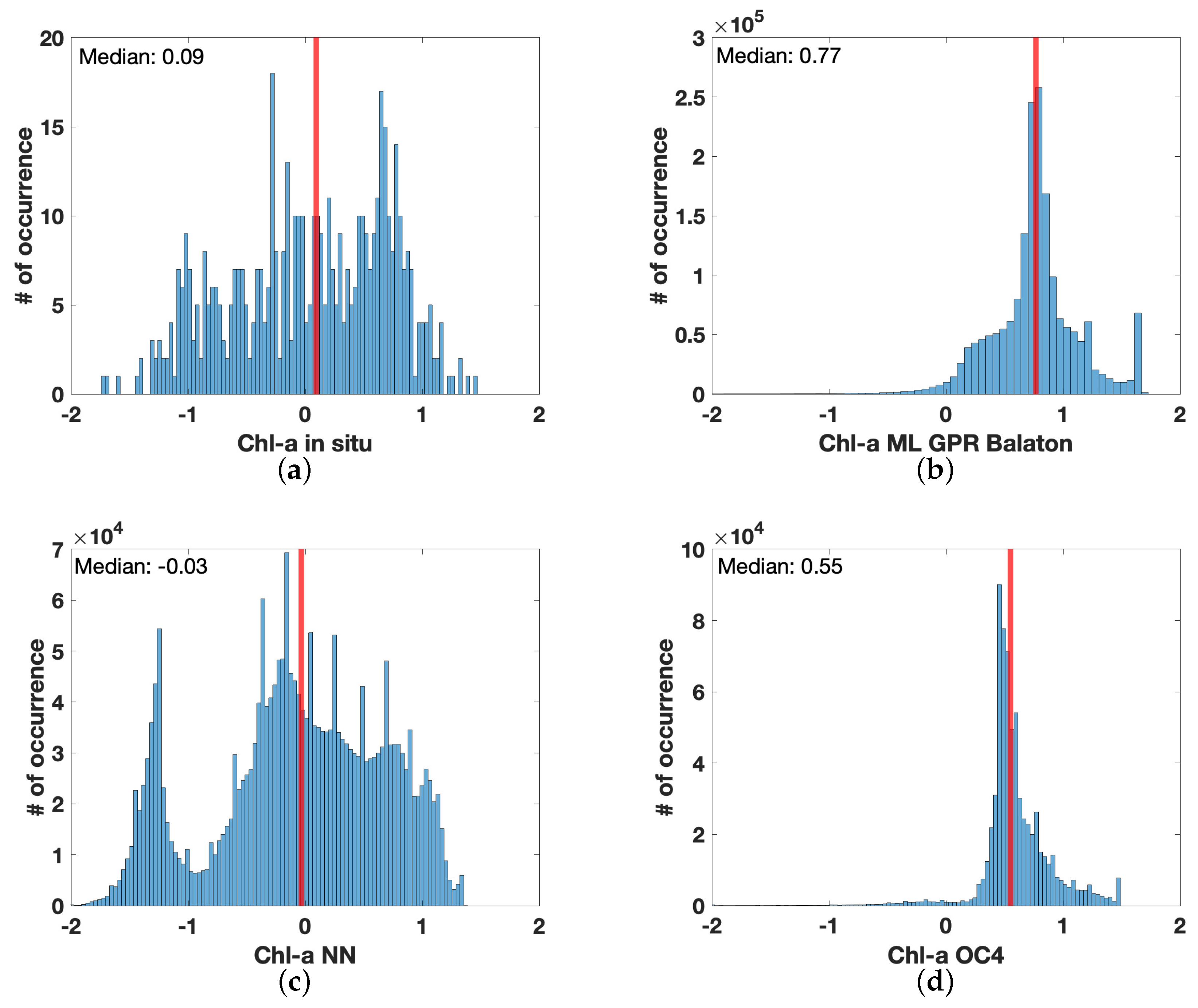
3.1. Statistical Analysis
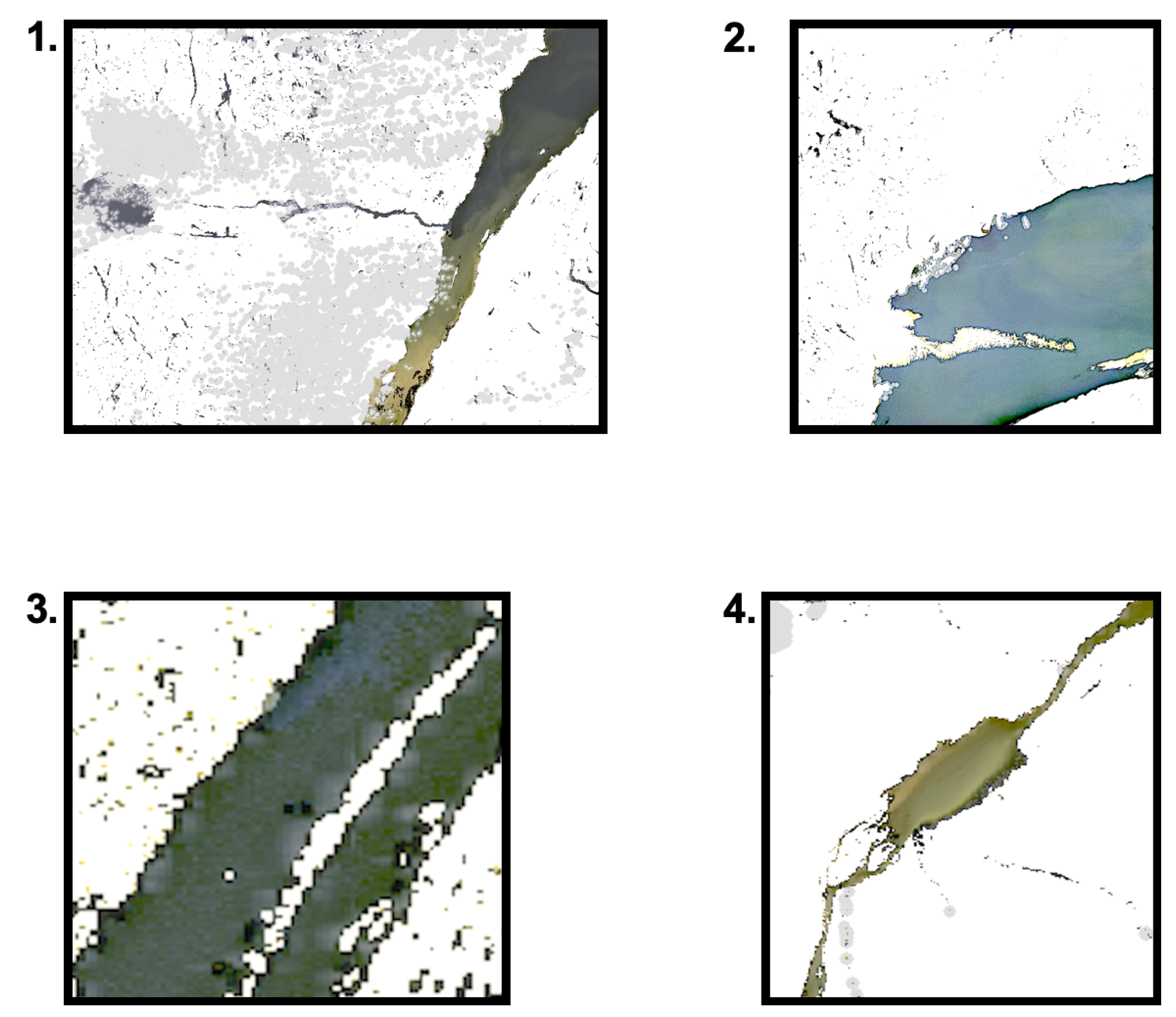
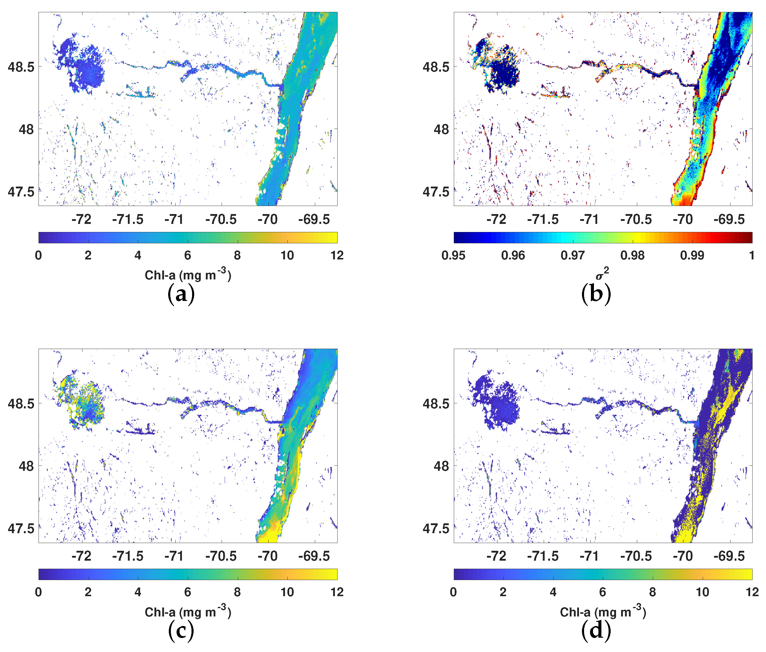
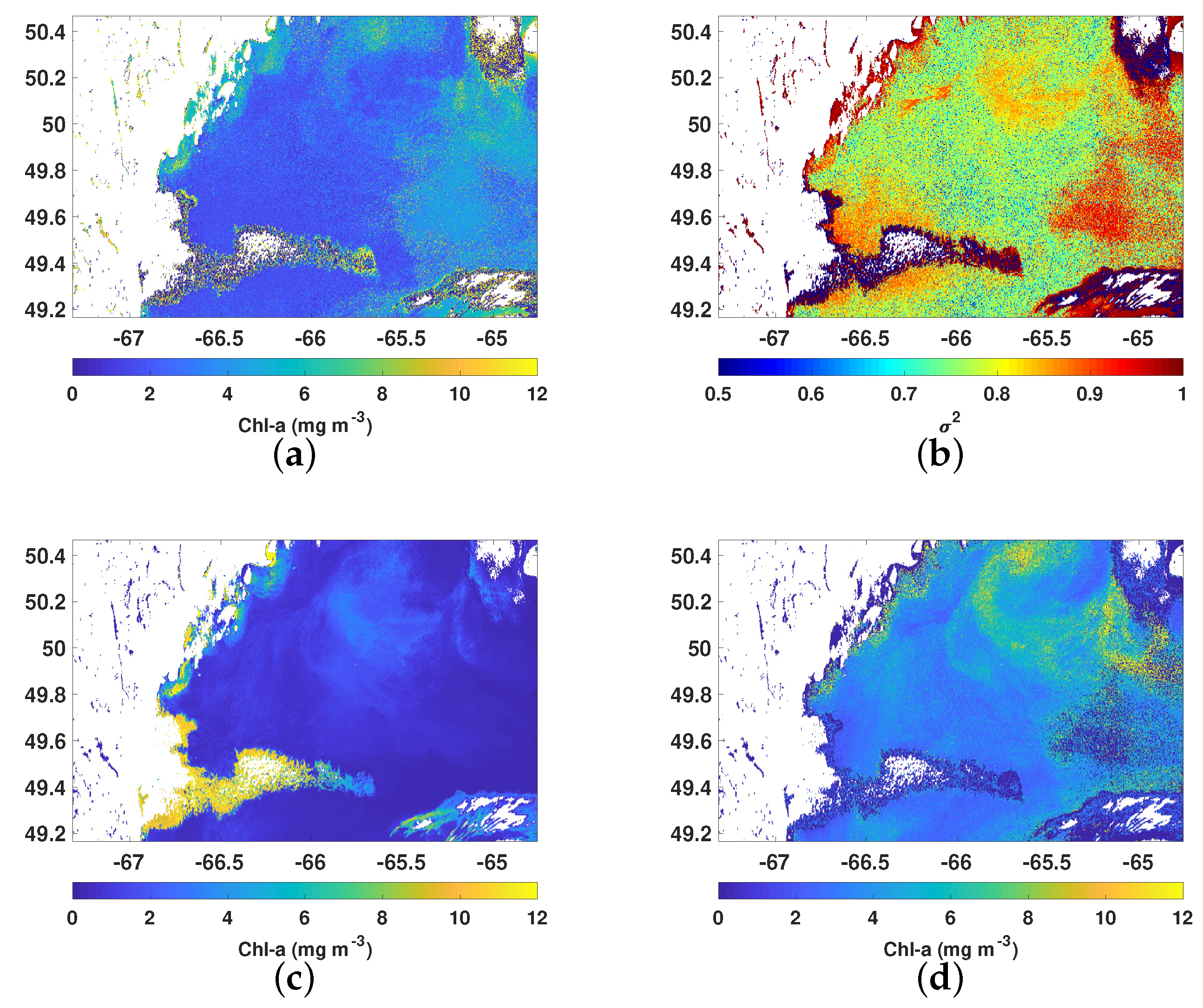
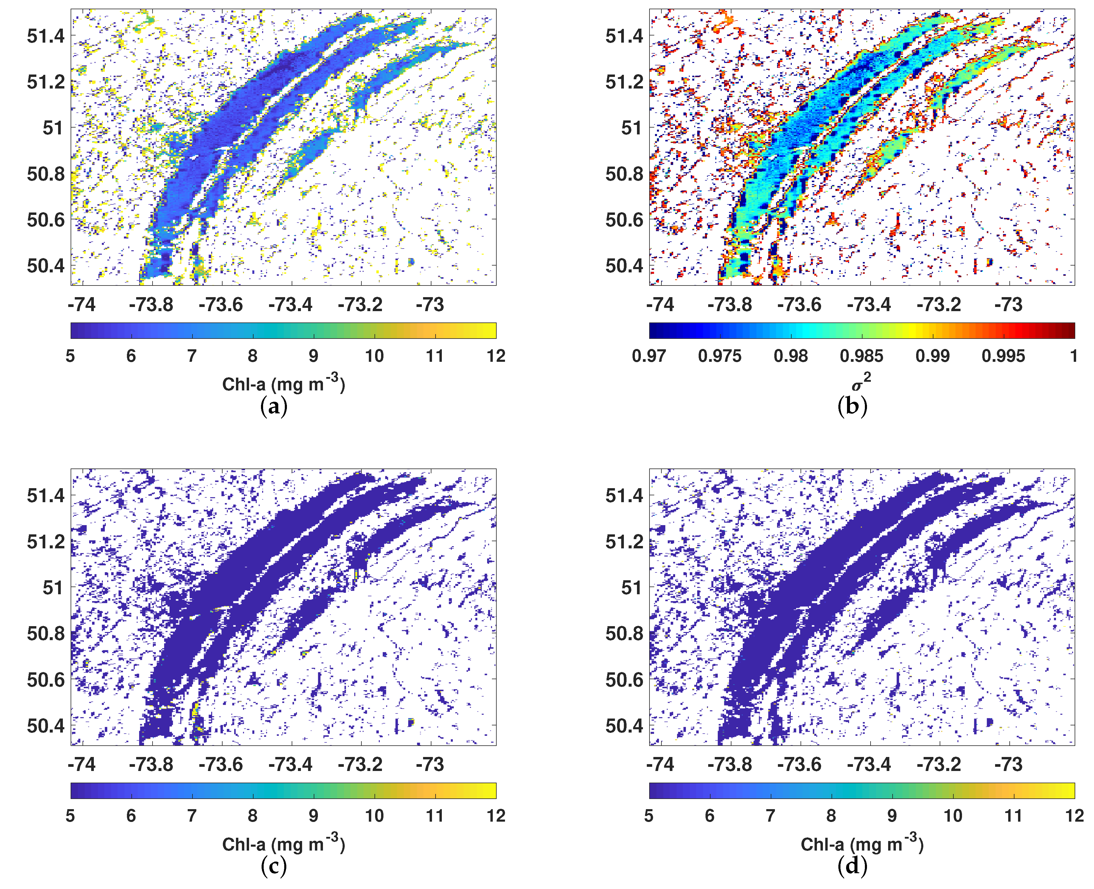
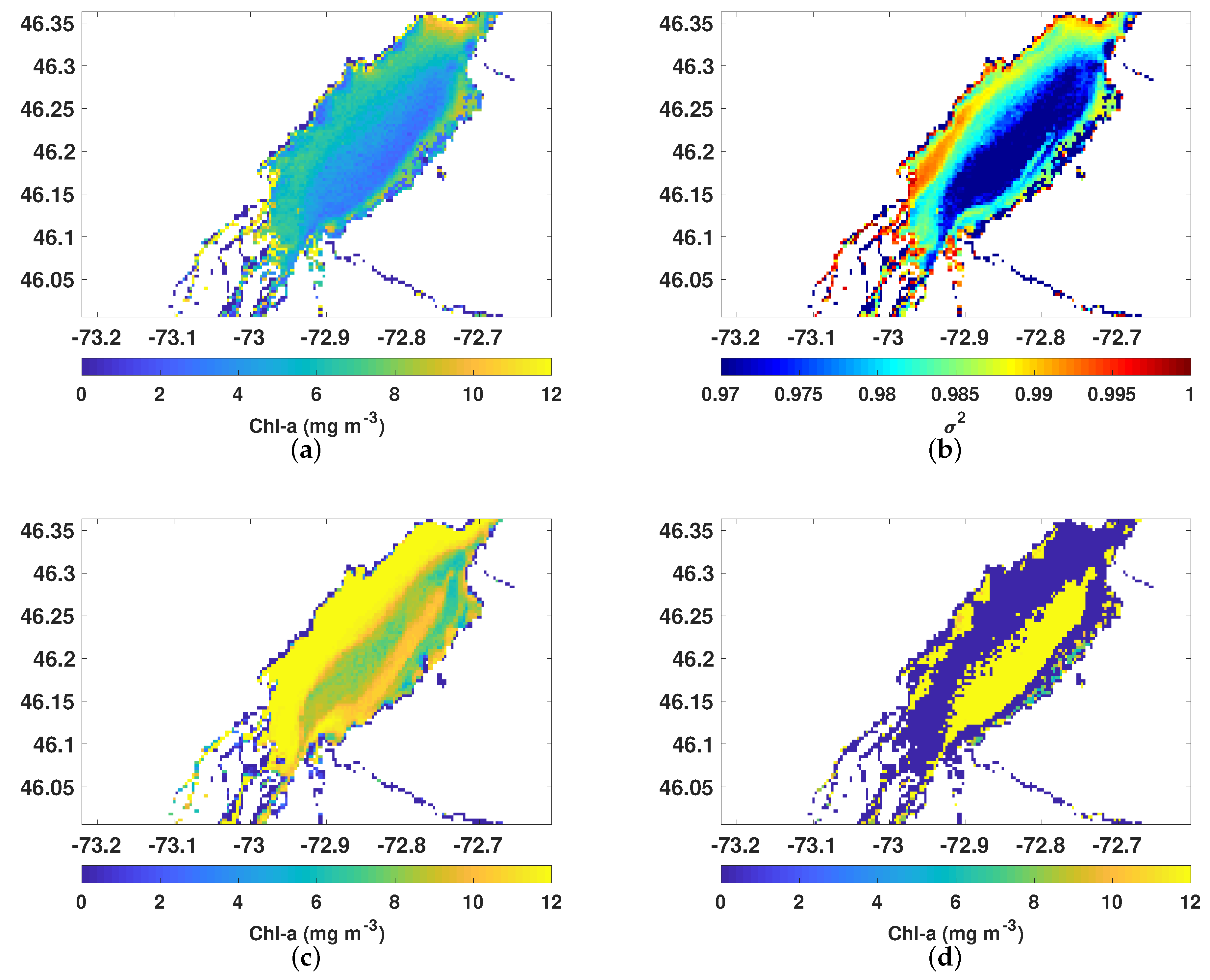
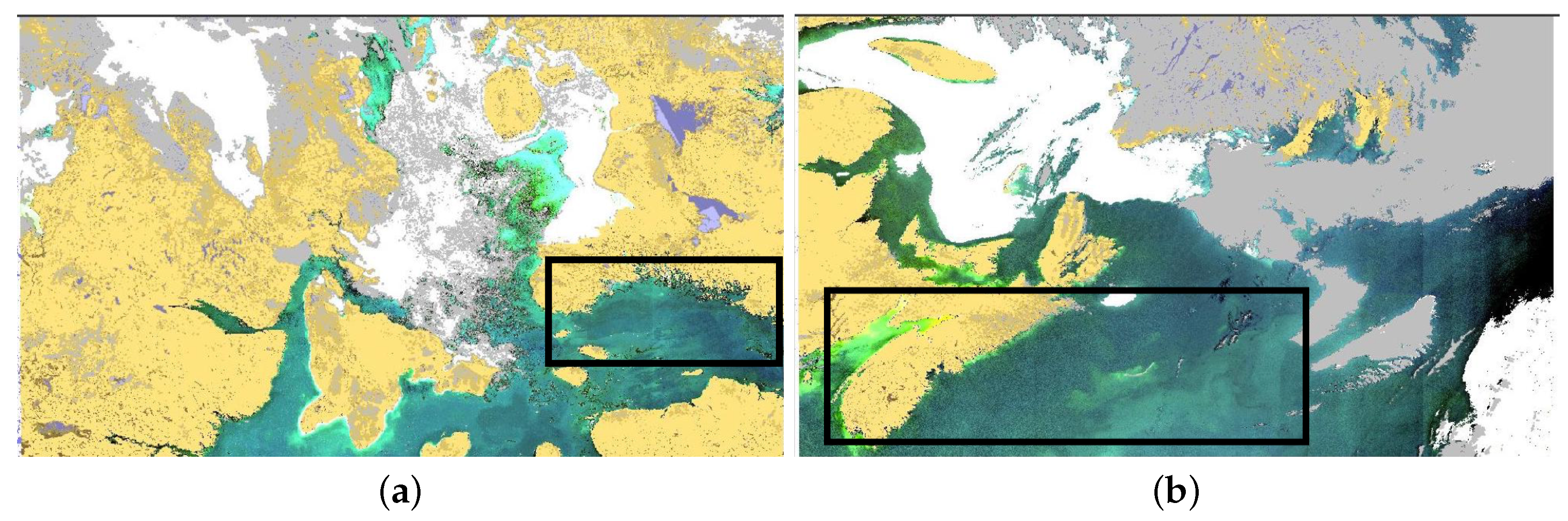
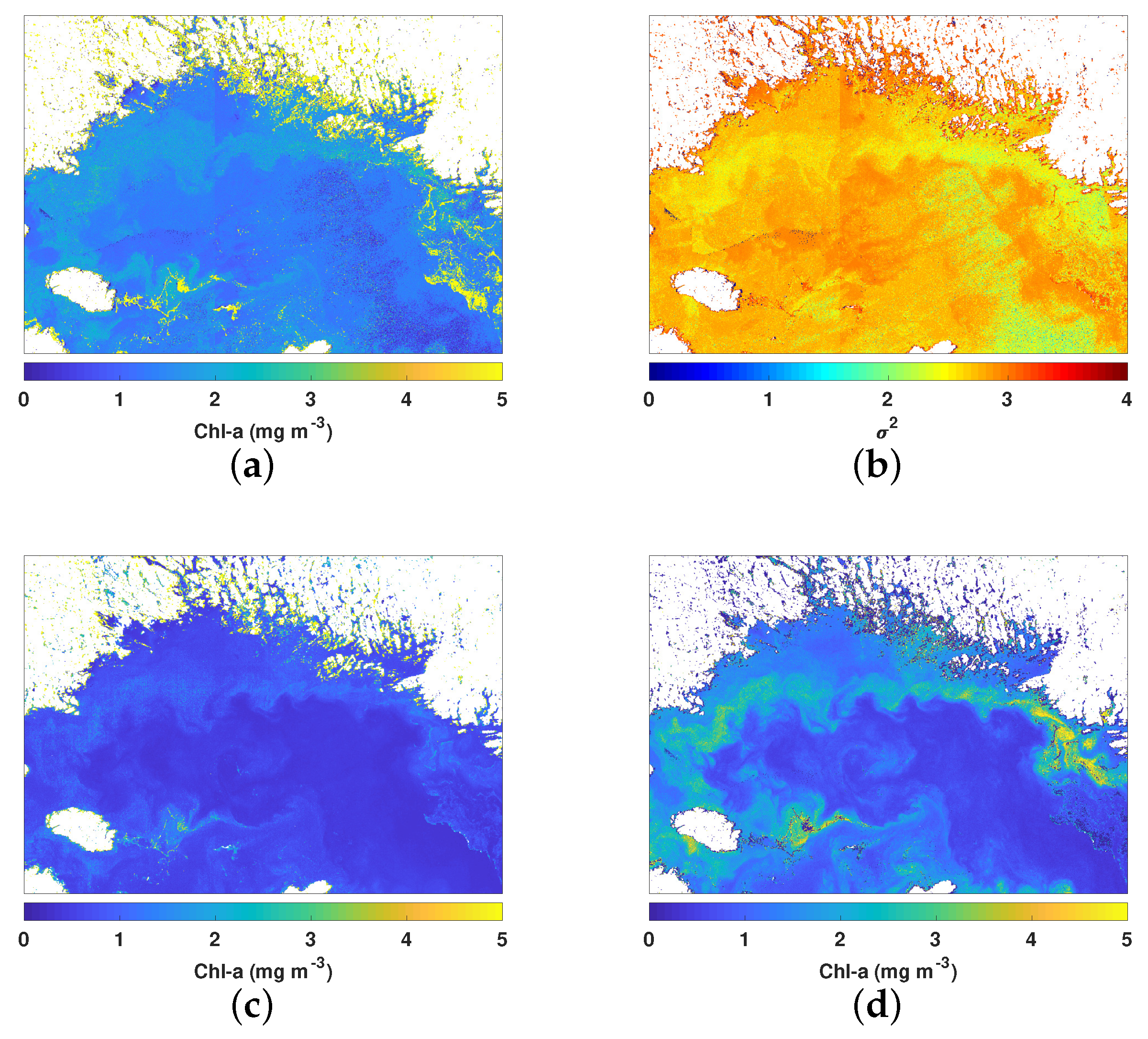
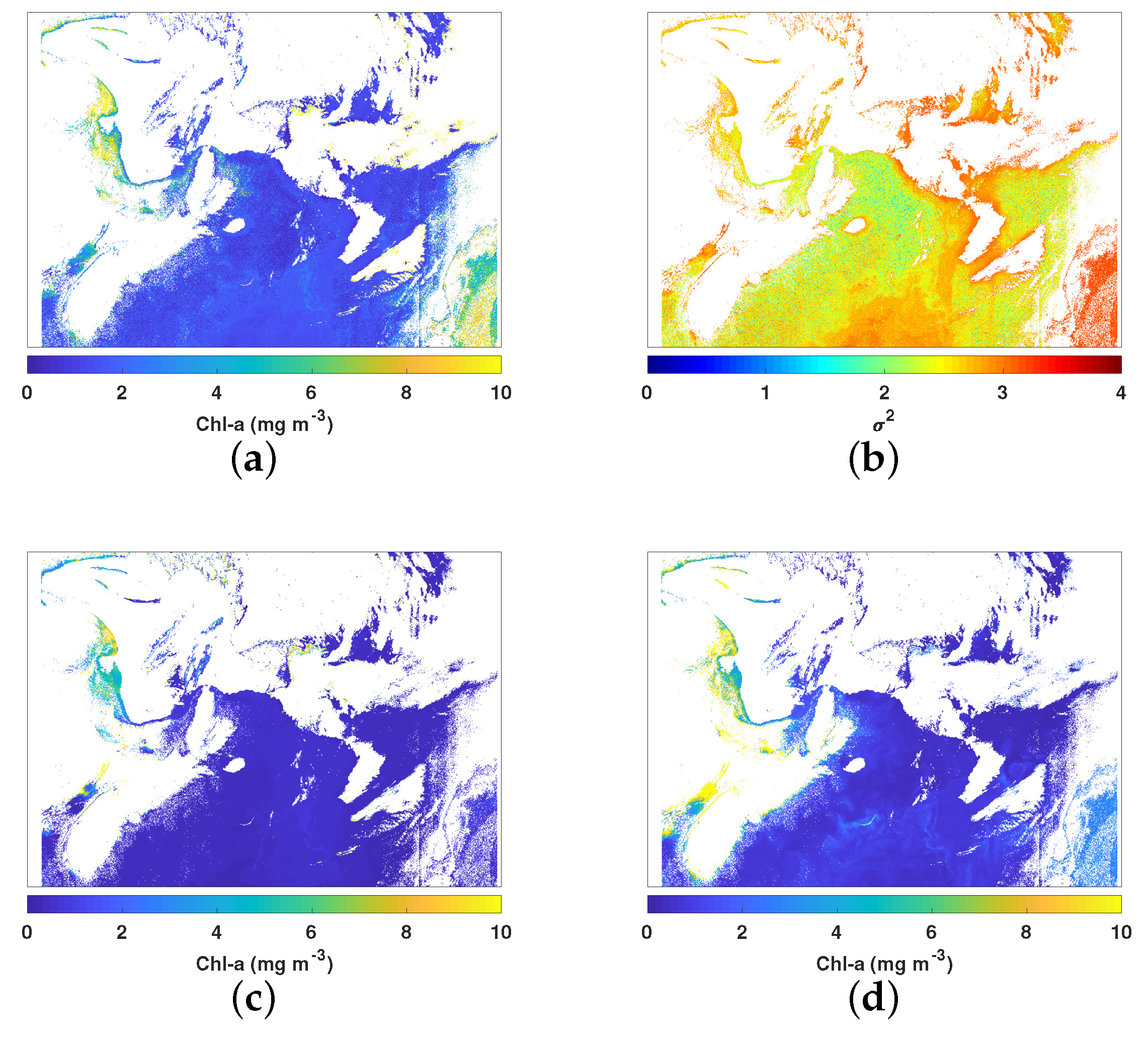
3.2. Chl-a Maps in High Northern Latitude Complex Waters
4. Discussions
5. Conclusions
Author Contributions
Funding
Acknowledgments
Conflicts of Interest
Appendix A. Chl-a Maps in the Marginal Ice Zone, Coastal, and Open Oceans


References
- Meier, W.N.; Hovelsrud, G.K.; van Oort, B.E.; Key, J.R.; Kovacs, K.M.; Michel, C.; Haas, C.; Granskog, M.A.; Gerland, S.; Perovich, D.K.; et al. Arctic sea ice in transformation: A review of recent observed changes and impacts on biology and human activity. Rev. Geophys. 2014, 52, 185–217. [Google Scholar] [CrossRef]
- Renaut, S.; Devred, E.; Babin, M. Northward Expansion and Intensification of Phytoplankton Growth During the Early Ice-Free Season in Arctic. Geophys. Res. Lett. 2018, 45, 10590–10598. [Google Scholar] [CrossRef]
- Ardyna, M.; Babin, M.; Gosselin, M.; Devred, E.; Rainville, L.; Tremblay, J.E. Recent Arctic Ocean sea ice loss triggers novel fall phytoplankton blooms. Geophys. Res. Lett. 2014, 41, 6207–6212. [Google Scholar] [CrossRef]
- Engelsen, O.; Hegseth, E.N.; Hop, H.; Hansen, E.; Falk-Pedersen, S. Spatial variability of chlorophyll-a on the Marginal Ice Zone of the Barents Sea, with relsations to sea ice and oceanographic conditions. J. Mar. Syst. 2002, 35, 79–97. [Google Scholar] [CrossRef]
- Volk, T.; Hoffert, M.I. Ocean Carbon Pumps: Analysis of Relative Strengths and Efficiencies in Ocean-Driven Atmospheric CO2 Changes; American Geophysical Union: Washington, DC, USA, 2013; pp. 99–110. [Google Scholar]
- Johannessen, O.M.; Miles, M.W. Critical vulnerabilities of marine and sea ice–based ecosystems in the high Arctic. Reg. Environ. Chang. 2011, 11, 239–248. [Google Scholar] [CrossRef]
- Arrigo, K.R.; Robinson, D.H.; Worthen, D.L.; Dunbar, R.B.; DiTullio, G.R.; VanWoert, M.; Lizotte, M.P. Phytoplankton Community Structure and the Drawdown of Nutrients and CO2 in the Southern Ocean. Science 1999, 283, 365–367. [Google Scholar] [CrossRef]
- Hein, M.; Sand-Jensen, K. CO2 increases oceanic primary production. Nature 1997, 388, 526–527. [Google Scholar] [CrossRef]
- Hofmann, M.; Worm, B.; Rahmstorf, S.; Schellnhuber, H.J. Declining ocean chlorophyll under unabated anthropogenic CO2 emissions. Environ. Res. Lett. 2011, 6, 034–035. [Google Scholar] [CrossRef]
- Bird, K.J.; Charpentier, R.R.; Gautier, D.L.; Houseknecht, D.W.; Klett, T.R.; Pitman, J.K.; Moore, T.E.; Schenk, C.J.; Tennyson, M.E.; Wandrey, C.J.; et al. Circum-Arctic Resource Appraisal: Estimates of Undiscovered Oil and Gas North of the Arctic Circle; U.S. Geological Survey Fact Sheet 2008; U.S. Geological Survey: Denver, CO, USA, 2008; pp. 1175–1179.
- Jacobsen, S.R.; Gudmestad, O.T. Evacuation From Petroleum Facilities Operating in the Barents Sea. In Proceedings of the ASME 2012 31st International Conference on Ocean, Offshore and Arctic Engineering, Rio de Janeiro, Brazil, 1–6 July 2012; Volume 6, pp. 457–466. [Google Scholar]
- Melia, N.; Haines, K.; Hawkins, E.; Day, J.J. Towards seasonal Arctic shipping route predictions. Environ. Res. Lett. 2017, 12, 084005. [Google Scholar] [CrossRef]
- Dawson, J.; Johnston, M.; Stewart, E. Governance of Arctic expedition cruise ships in a time of rapid environmental and economic change. Ocean. Coast. Manag. 2014, 89, 88–99. [Google Scholar] [CrossRef]
- Choudhury, S.B.; Jena, B.; Rao, M.V.; Rao, K.H.; Somvanshi, V.S.; Gulati, D.K.; Sahu, S.K. Validation of integrated potential fishing zone (IPFZ) forecast using satellite based chlorophyll and sea surface temperature along the east coast of India. Int. J. Remote. Sens. 2007, 28, 2683–2693. [Google Scholar] [CrossRef]
- Hommedal, S.; Lorentzen, E.A. What We Know about the So-Called Killer Alga in Northern Norway. 2019. Available online: http://www.imr.no/en/hi/news/2019/may/what-we-know-about-the-so-called-killer-alga-in-northern-norway (accessed on 3 September 2019).
- Wauthy, M.; Rautio, M.; Christoffersen, K.S.; Forsström, L.; Laurion, I.; Mariash, H.L.; Peura, S.; Vincent, W.F. Increasing dominance of terrigenous organic matter in circumpolar freshwaters due to permafrost thaw. Limnol. Oceanogr. Lett. 2018, 3, 186–198. [Google Scholar] [CrossRef]
- MODIS-Aqua. Available online: https://modis.gsfc.nasa.gov/ (accessed on 25 June 2019).
- VIIRS. Available online: https://jointmission.gsfc.nasa.gov/ (accessed on 3 September 2019).
- Landsat-8 OLI. Available online: https://landsat.gsfc.nasa.gov/operational-land-imager-oli/ (accessed on 3 September 2019).
- Sentinel 2 MSI. Available online: https://sentinel.esa.int/web/sentinel/missions/sentinel-2 (accessed on 3 September 2019).
- Sentinel 3 OLCI. Available online: https://sentinels.copernicus.eu/web/sentinel/missions/sentinel-3 (accessed on 3 September 2019).
- O’Reilly, J.E.; Maritirena, S.; Mitchell, B.G.; Siegel, D.A.; Carder, K.L.; Garver, S.A.; Kahru, M.; McClain, C. Ocean color chlorophyll algorithms for SeaWiFS. J. Geophys. Res. 1998, 103, 24937–24953. [Google Scholar] [CrossRef]
- Morel, A.; Claustre, H.; Antoine, D.; Gentili, B. Natural variability of bio-optical properties in Case 1 waters: attenuation and reflectance within the visible and near-UV spectral domains, as observed in South Pacific and Mediterranean waters. Biogeosciences 2007, 4, 913–925. [Google Scholar] [CrossRef]
- Doerffer, R.; Schiller, H. The MERIS Case 2 water algorithm. Int. J. Remote. Sens. 2007, 28, 517–535. [Google Scholar] [CrossRef]
- Brockmann, C.; Doerffer, R.; Peters, M.; Kerstin, S.; Embacher, S.; Ruescas, A. Evolution of the C2RCC Neural Network for Sentinel 2 and 3 for the Retrieval of Ocean Colour Products in Normal and Extreme Optically Complex Waters. In Proceedings of the Living Planet Symposium, Prague, Czech Republic, 9–13 May 2016; ESA Special Publication: Noordwijk, The Netherlands, 2016; Volume 740, p. 54. [Google Scholar]
- Blix, K.; Pálffy, K.; Tóth, V.R.; Eltoft, T. Remote Sensing of Water Quality Parameters over Lake Balaton by Using Sentinel-3 OLCI. Water 2018, 10, 1428. [Google Scholar] [CrossRef]
- Fan, Y.; Li, W.; Voss, K.J.; Gatebe, C.K.; Stamnes, K. Neural network method to correct bidirectional effects in water-leaving radiance. Appl. Opt. 2016, 55, 10–21. [Google Scholar] [CrossRef]
- Fan, Y.; Li, W.; Gatebe, C.K.; Jamet, C.; Zibordi, G.; Schroeder, T.; Stamnes, K. Atmospheric correction over coastal waters using multilayer neural networks. Remote. Sens. Environ. 2017, 199, 218–240. [Google Scholar] [CrossRef]
- Cipollini, P.; Corsini, G.; Diani, M.; Grass, R. Retrieval of sea water optically active parameters from hyperspectral data by means of generalized radial basis function neural networks. IEEE Trans. Geosci. Remote. Sens. 2001, 39, 1508–1524. [Google Scholar] [CrossRef]
- Hieronymi, M.; Müller, D.; Doerffer, R. The OLCI Neural Network Swarm (ONNS): A Bio-Geo-Optical Algorithm for Open Ocean and Coastal Waters. Front. Mar. Sci. 2017, 4, 140. [Google Scholar] [CrossRef]
- Zhan, H.; Shi, P.; Chen, C. Retrieval of Oceanic Chlorophyll Concentration Using Support Vector Machines. IEEE Trans. Geosci. Remote. Sens. 2003, 41, 2947–2951. [Google Scholar] [CrossRef]
- Kwiatkowska, E.J.; Fargion, G.S. Application of Machine-Learning Techniques Toward the Creation of a Consistent and Calibrated Global Chlorophyll Concentration Baseline Dataset Using Remotely Sensed Ocean Color Data. IEEE Trans. Geosci. Remote. Sens. 2003, 41, 2844–2860. [Google Scholar] [CrossRef]
- Camps-Valls, G.; Muñoz-Marí, J.L.; Gómez-Chova, K.R.; Calpe-Maravilla, J. Biophysical Parameter Estimation With a Semisupervised Support Vector Machine. IEEE Geosci. Remote. Sens. Lett. 2009, 6, 248–252. [Google Scholar] [CrossRef]
- Camps-Valls, G.; Gómez-Chova, L.; Muñoz-Marí, J.; Vila-Francés, J.; Amorós-López, J.; Calpe-Maravilla, J. Retrieval of oceanic chlorophyll concentration with relevance vector machines. Remote. Sens. Environ. 2006, 105, 23–33. [Google Scholar] [CrossRef]
- Pasolli, L.; Melgani, F.; Blanzieri, E. Gaussian Process Regression for Estimating Chlorophyll Concentration in Subsurface Waters From Remote Sensing Data. IEEE Geosci. Remote. Sens. Lett. 2010, 7, 464–468. [Google Scholar] [CrossRef]
- Verrelst, J.; Muñoz, J.; Alonso, L.; Rivera, J.P.; Camps-Valls, G.; Moreno, J. Machine learning regression algorithms for biophysical parameter retrieval: Opportunities for Sentinel-2 and -3. Remote. Sens. Environ. 2012, 118, 127–139. [Google Scholar] [CrossRef]
- Verrelst, J.; Alonso, L.; Camps-Valls, G.; Delegido, J.; Moreno, J. Retrieval of Vegetation Biophysical Parameters Using Gaussian Process Techniques. IEEE Trans. Geosci. Remote. Sens. 2012, 50, 1832–1843. [Google Scholar] [CrossRef]
- Blix, K.; Camps-Valls, G.; Jenssen, R. Gaussian Process Sensitivity Analysis for Oceanic Chlorophyll Estimation. IEEE J. Sel. Top. Appl. Earth Obs. Remote. Sens. 2017, 10, 1265–1277. [Google Scholar] [CrossRef]
- Blix, K.; Eltoft, T. Evaluation of feature ranking and regression methods for oceanic chlorophyll-a estimation. IEEE J. Sel. Top. Appl. Earth Obs. Remote. Sens. 2018, 11, 1403–1418. [Google Scholar] [CrossRef]
- Blix, K.; Eltoft, T. Machine Learning Automatic Model Selection Algorithm for Oceanic Chlorophyll-a Content Retrieval. Remote. Sens. 2018, 10, 775. [Google Scholar] [CrossRef]
- Blix, K.; Eltoft, T. A Generalized Chlorophyll-a Estimation Model for Complexity-Diverse Arctic Waters. In Proceedings of the 2019 IEEE International Geoscience and Remote Sensing Symposium (IGARSS 2019), Yokohama, Japan, 28 July–2 August 2019. [Google Scholar]
- MALINA Data. Available online: http://www.obs-vlfr.fr/proof/php/malina/ (accessed on 5 March 2019).
- ICESCAPE Data. Available online: https://seabass.gsfc.nasa.gov/ (accessed on 3 September 2019).
- TARA Data. Available online: https://oceans.taraexpeditions.org/ (accessed on 3 September 2019).
- GREEN EDGE Data. Available online: http://www.obs-vlfr.fr/proof/php/GREENEDGE/ (accessed on 3 September 2019).
- Morrow, J.H.; Hooker, S.B.; Booth, C.R.; Bernhard, G.; Lind, R.N.; Brown, J. Advances in Measuring the Apparent Optical Properties (AOPs) of Optically Complex Waters. NASA Tech. Memo 2010, 215856, 42–50. [Google Scholar]
- Hooker, S.B.; Morrow, J.H.; Matsuoka, A. Apparent optical properties of the Canadian Beaufort Sea—Part 2: 1 % and 1 cm perspective in deriving and validating AOP data products. Biogeosciences 2013, 10, 4511–4527. [Google Scholar] [CrossRef]
- Gordon, H.R.; Ding, K. Self-shading of in-water optical instruments. Limnol. Oceanogr. 1992, 37, 491–500. [Google Scholar] [CrossRef]
- Babin, M.; Morel, A.; Fournier-Sicre, V.; Fell, F.; Stramski, D. Light scattering properties of marine particles in coastal and open ocean waters as related to the particle mass concentration. Limnol. Oceanogr. 2003, 48, l843–859. [Google Scholar] [CrossRef]
- Bélanger, S.; Babin, M.; Larouche, P. An empirical ocean color algorithm for estimating the contribution of chromophoric dissolved organic matter to total light absorption in optically complex waters. J. Geophys. Res. Ocean. 2008, 113. [Google Scholar] [CrossRef]
- Ras, J.; Claustre, H.; Uitz, J. Spatial variability of phytoplankton pigment distributions in the Subtropical South Pacific Ocean: comparison between in situ and predicted data. Biogeosciences 2008, 5, 353–369. [Google Scholar] [CrossRef]
- Heukelem, L.V.; Thomas, C.S. Computer-assisted high-performance liquid chromatography method development with applications to the isolation and analysis of phytoplankton pigments. Chromatogr. A 2001, 910, 31–49. [Google Scholar] [CrossRef]
- Matsuoka, A.; Boss, E.; Babin, M.; Karp-Boss, L.; Hafez, M.; Chekalyuk, A.; Proctor, C.W.; Werdell, P.J.; Bricaud, A. Pan-Arctic optical characteristics of colored dissolved organic matter: Tracing dissolved organic carbon in changing Arctic waters using satellite ocean color data. Remote. Sens. Environ. 2017, 200, 89–101. [Google Scholar] [CrossRef]
- Massicotte, P.; Gratton, D.; Frenette, J.J.; Assani, A.A. Spatial and temporal evolution of the St. Lawrence River spectral profile: A 25-year case study using Landsat 5 and 7 imagery. Remote. Sens. Environ. 2013, 136, 433–441. [Google Scholar] [CrossRef]
- Rasmussen, C.E.; Williams, C.K.I. Gaussian Processes for Machine Learning; The MIT Press: Cambridge, MA, USA, 2005. [Google Scholar]
- Ahmad, Z.; Franz, B.A.; McClain, C.R.; Kwiatkowska, E.J.; Werdell, J.; Shettle, E.P.; Holben, B.N. New aerosol models for the retrieval of aerosol optical thickness and normalized water-leaving radiances from the SeaWiFS and MODIS sensors over coastal regions and open oceans. Appl. Opt. 2010, 49, 5545–5560. [Google Scholar] [CrossRef]
- Bailey, S.W.; Werdell, P.J. A multi-sensor approach for the on-orbit validation of ocean color satellite data products. Remote. Sens. Environ. 2006, 102, 12–23. [Google Scholar] [CrossRef]
- Gordon, H.R.; Wang, M. Influence of oceanic whitecaps on atmospheric correction of ocean-color sensors. Appl. Opt. 1994, 33, 7754–7763. [Google Scholar] [CrossRef] [PubMed]
- Zibordi, G.; Mélin, F.; Berthon, J.F. Comparison of SeaWiFS, MODIS and MERIS radiometric products at a coastal site. Geophys. Res. Lett. 2006, 33. [Google Scholar] [CrossRef]
- Liang, L.; Qin, Z.; Zhao, S.; Di, L.; Zhang, C.; Deng, M.; Lin, H.; Zhang, L.; Wang, L.; Liu, Z. Estimating crop chlorophyll content with hyperspectral vegetation indices and the hybrid inversion method. Int. J. Remote. Sens. 2016, 37, 2923–2949. [Google Scholar] [CrossRef]
- Watanabe, F.; Alcântara, E.; Imai, N.; Rodrigues, T.; Bernardo, N. Estimation of Chlorophyll-a Concentration from Optimizing a Semi-Analytical Algorithm in Productive Inland Waters. Remote. Sens. 2018, 10, 227. [Google Scholar] [CrossRef]
- Lins, R.C.; Martinez, J.M.; Motta Marques, D.D.; Cirilo, J.A.; Fragoso, C.R. Assessment of Chlorophyll-a Remote Sensing Algorithms in a Productive Tropical Estuarine-Lagoon System. Remote. Sens. 2017, 9, 516. [Google Scholar] [CrossRef]


| Cruise | Nr. of Samples | Date | Area |
|---|---|---|---|
| MALINA | 35 | 30 July 2009–26 August 2009 | Southern Beaufort Sea |
| ICESCAPE2010 | 18 | 15 June 2010–22 July 2010 | Chukchi and Beaufort Sea |
| ICESCAPE2011 | 37 | 25 June 2011–29 July 2011 | Chukchi and Beaufort Sea |
| TARA | 28 | 24 May 2013–5 November 2013 | Kara and Laptev Sea |
| GREEN EDGE | 31 | 24 June 2016–10 July 2016 | Baffin Bay |
© 2019 by the authors. Licensee MDPI, Basel, Switzerland. This article is an open access article distributed under the terms and conditions of the Creative Commons Attribution (CC BY) license (http://creativecommons.org/licenses/by/4.0/).
Share and Cite
Blix, K.; Li, J.; Massicotte, P.; Matsuoka, A. Developing a New Machine-Learning Algorithm for Estimating Chlorophyll-a Concentration in Optically Complex Waters: A Case Study for High Northern Latitude Waters by Using Sentinel 3 OLCI. Remote Sens. 2019, 11, 2076. https://doi.org/10.3390/rs11182076
Blix K, Li J, Massicotte P, Matsuoka A. Developing a New Machine-Learning Algorithm for Estimating Chlorophyll-a Concentration in Optically Complex Waters: A Case Study for High Northern Latitude Waters by Using Sentinel 3 OLCI. Remote Sensing. 2019; 11(18):2076. https://doi.org/10.3390/rs11182076
Chicago/Turabian StyleBlix, Katalin, Juan Li, Philippe Massicotte, and Atsushi Matsuoka. 2019. "Developing a New Machine-Learning Algorithm for Estimating Chlorophyll-a Concentration in Optically Complex Waters: A Case Study for High Northern Latitude Waters by Using Sentinel 3 OLCI" Remote Sensing 11, no. 18: 2076. https://doi.org/10.3390/rs11182076
APA StyleBlix, K., Li, J., Massicotte, P., & Matsuoka, A. (2019). Developing a New Machine-Learning Algorithm for Estimating Chlorophyll-a Concentration in Optically Complex Waters: A Case Study for High Northern Latitude Waters by Using Sentinel 3 OLCI. Remote Sensing, 11(18), 2076. https://doi.org/10.3390/rs11182076