Article

Latent Heat Flux in the Agulhas Current

by
Arielle Stela Imbol Nkwinkwa N.
1,2,3,*,
Mathieu Rouault
1,2 and
Johnny A. Johannessen
4
1
Department of Oceanography, Ma-Re Institute, University of Cape Town, Cape Town 7701, South Africa
2
Nansen Tutu Center for Marine Environmental Research, University of Cape Town, Cape Town, 7701 South Africa
3
GEOMAR Helmholtz Centre for Ocean Research Kiel, 2405 Kiel, Germany
4
Nansen Environmental and Remote Sensing Research Center and Geophysical Institute, University of Bergen, N-5006 Bergen, Norway
*
Author to whom correspondence should be addressed.
Remote Sens. 2019, 11(13), 1576; https://doi.org/10.3390/rs11131576
Submission received: 29 April 2019 / Revised: 21 June 2019 / Accepted: 24 June 2019 / Published: 3 July 2019
(This article belongs to the Special Issue Remote Sensing of Ocean-Atmosphere Interactions)

Abstract

:
In-situ observation, climate reanalyses, and satellite remote sensing are used to study the annual cycle of turbulent latent heat flux (LHF) in the Agulhas Current system. We assess if the datasets do represent the intense exchange of moisture that occurs above the Agulhas Current and the Retroflection region, especially the new reanalyses as the former, the National Centers for Environmental Prediction Reanalysis 2 (NCEP2) and the European Centre for Medium-Range Weather Forecast (ECMWF) reanalysis second-generation reanalysis (ERA-40) have lower sea and less distinct surface temperature (SST) in the Agulhas Current system due to their low spatial resolution thus do not adequately represent the Agulhas Current LHF. We use monthly fields of LHF, SST, surface wind speed, saturated specific humidity at the sea surface (Qss), and specific humidity at 10 m (Qa). The Climate Forecast System Reanalysis (CFSR), the European Centre for Medium-Range Weather Forecast fifth generation (ERA-5), and the Modern-Era Retrospective analysis for Research and Applications version-2 (MERRA-2) are similar to the air–sea turbulent fluxes (SEAFLUX) and do represent the signature of the Agulhas Current. ERA-Interim underestimates the LHF due to lower surface wind speeds than other datasets. The observation-based National Oceanography Center Southampton (NOCS) dataset is different from all other datasets. The highest LHF of 250 W/m2 is found in the Retroflection in winter. The lowest LHF (~100 W/m2) is off Port Elizabeth in summer. East of the Agulhas Current, Qss-Qa is the main driver of the amplitude of the annual cycle of LHF, while it is the wind speed in the Retroflection and both Qss-Qa and wind speed in between. The difference in LHF between product are due to differences in Qss-Qa wind speed and resolution of datasets.

Graphical Abstract

1. Introduction

The greater Agulhas Current system is composed of the core of the Agulhas Current, which is about 219 km wide near 34°S [1]; the Agulhas Retroflection region with a loop diameter of 350 km [2]; and the Agulhas Return Current that meanders back in an eastward direction [3] (Figure 1). The core of the Agulhas Current is steered by the shelf break (200 m isobaths) along the southeast coast of South Africa. It is the strongest western boundary current in the Southern Hemisphere. The mean position of the Agulhas Retroflection lies between 16° and 20°E and between 38° and 41°S [2]. The Agulhas current takes warm water poleward creating a distinct signature in SST along its path. This SST gradient is at the origin of the high turbulent flux of sensible and latent heat observed above the current and creates a wall of moisture above the current with distinct cloud lines observed at time above it [3,4]. As the Agulhas Current follows the coast of South Africa, offshore wind can bring this moisture inland [5,6]. The SST gradient is also at the origin of increased rainfall above the current and near the coast of South Africa [7] and also wind increase [8,9,10] or wind curl change above the current [11]. The LHF, as well as marine boundary layer modification, were measured above the core of the Agulhas Current, the Retroflection region and the Agulhas Return Current [4,5,12,13,14,15,16]. These measurements show that the LHF, which is akin to the turbulent flux of moisture at the air–sea interface, is higher in the Agulhas Current system compared to the surrounding ocean. The core of the Agulhas Current is important because of its thermal contrast with the surrounding water leading to a fivefold increase in the turbulent fluxes of latent heat. Radiosondes launched during the Agulhas Current air–sea exchange experiment (ACASEX) cruise show that the core of the current produces a wall of moisture [4,5,13] that can reach up to 2000 m above the Agulhas Current. When the wind is blowing from the Agulhas Current to the coast, this moisture converges towards the coast [5,6,13]. Cloud lines above the Agulhas Current are the results of the strong exchange of moisture and mixing occurring in this region [3,5,17].
The study of Rouault [18] provided evidence that low-level moisture from the Agulhas Current played a significant role in the evolution of a severe convective storm and associated tornado over southern South Africa. In addition, this strong western boundary current has warmed up considerably since the 1980s, which has increased the transfer of moisture from the ocean to the atmosphere [19]. However, more need to be done to understand the impact of that recent increase in moisture on the weather and climate of the region. Gimeno et al. [20] showed that the Agulhas Current system is a source of moisture for the Southern Africa rainfall although the low-resolution of data might have underestimated the intensity of the ocean to atmosphere exchanges in the core of the Agulhas Current as they used the ECMWF second-generation reanalysis (ERA-40 [21]) with a spatial resolution of 2.5° × 2.5°. Indeed the LHF is underestimated in models if the resolution does not represent the SST well the Agulhas Current which is roughly 100 km wide [16]. In addition the high latent and sensible heat flux modify the stability of the surface constant flux layer and the associated logarithmic profile of wind speed temperature and humidity at the surface of the ocean. This creates a difference pressure gradient found to be the origin of low-level convection and rainfall above the Agulhas Current by Nkwinkwa Njouodo et al. [7]).
As stated above, the LHF measured over the Agulhas Current were not well reproduced in older climate reanalyses (ERA-40 [21], the Centers for Environmental Prediction version 1 (NCEP1 [22]) and version 2 (NCEP2 [23])). However, recent reanalyses like the Climate Forecast System Reanalysis (CFSR [24]) are now available at a higher resolution. Similarly, numerous new air–sea interaction data sets derived from satellite remote sensing such as air–sea turbulent fluxes (SEAFLUX [25]) have been produced at a resolution to allow a good representation of the Agulhas Current.
The aims of this study of the air–sea exchanges in the Agulhas Current system are threefold: (i) to explore whether the new climate reanalyses and satellite-derived data sets do adequately represent the high LHF or exchange of moisture above the Agulhas Current, (ii) to examine the magnitude of uncertainties in the basic parameters (wind, SST, surface specific humidity) used to derive the LHF; and (iii) to quantify the annual cycle of the LHF and its drivers in the Agulhas Current system.

2. Data and Methods

Table 1 provides an overview of the eleven monthly data sets used. They are classified according to the input data sources and analysis methods (e.g., in-situ observations, satellite-based data sets, and reanalyses) together with an indication of the spatial resolution and record lengths. Various parameters are analysed here including geostrophic current; LHF; sea surface temperature (SST); surface wind speed at 10 m; specific humidity of air at 10 m (Qa) and specific humidity at sea surface (Qss).
The averaging periods that we performed range from monthly to seasonal and were constrained by the availability of satellite data sets. Because products were not available at the same period, we used the same common period (5 years from 2003 to 2007) for the averaging to have consistent results except for HOAPS3, available only until 2005.

2.1. In-Situ Observations

We analysed the gridded monthly data derived from the National Oceanography Centre Southampton (NOCS, version 2) based on Voluntary Observing Ship (VOS) obtained from the International Comprehensive Ocean-Atmosphere Data Set (ICOADS) [26,27,28]. These observations were presented on a 1° × 1° spatial grid and used optimal interpolation (OI) of daily estimates of ship data, which covered the period 1973–2006. The OI is based on the approach developed by Reynolds and Smith [29] and by Lornec [30]. The wind speeds over the oceans by the VOS were either visual estimates using the WMO1100 Beaufort Equivalent Scale [31] or from anemometers [27]. The anemometer observations were adjusted to a standard reference height of 10 m using the bulk formulae and parameterisations of Smith [32,33]. The temperatures of water samples were used to measure the SST by using a bucket or from the engine room intake (ERI). Corrections were applied for the different measurement methods [34]. Humidity observations were made using wet and dry bulb thermometers [27] and were adjusted to 10 m using Smith [32,33]. The flux estimates in the NOCS data were based on the bulk formulas of Smith [32,33]. A successive correction method was then used to develop the monthly NOCS flux fields [35].

2.2. Satellite Remote Sensing

Two satellite-based data products were used, notably the third version of the Hamburg Ocean Atmosphere Parameters and Fluxes (HOAPS3) product and the high-resolution SEAFLUX [25,36] product. The HOAPS3 product with a spatial resolution of 0.50° × 0.50° provided fields of turbulent heat fluxes over the global ice-free ocean. It was a completely reprocessed data set [37,38] with a continuous time series from 1987 to 2005. Our study period for HOAPS3 is from 2003 to 2005. The HOAPS3 wind speed was based on neural network algorithms. The SST was based on the Advanced Very High-Resolution Radiometer (AVHRR) Oceans Pathfinder SST [39]. Qss was calculated from the saturation humidity at the sea surface temperature using the Magnus formula [40], and Qa was calculated using the method implemented by Bentamy et al. [41]. HOAPS3 LHF was calculated from swath retrievals and parameterized using the Coupled Ocean-Atmosphere Response Experiment bulk flux algorithm version 3 (COARE3.0 [42]). We use the monthly data from HOAPS3. For SEAFLUX product, a general discussion of flux measurement issues is given in Curry et al. [25]. SEAFLUX benefits from an international effort under the GEWEX and CLIVAR umbrella [25]. SEAFLUX is a high-resolution (0.25° × 0.25°) satellite-based data set of surface turbulent fluxes over the global ocean, available from 1998 to 2007. SEAFLUX provides necessary parameters used to calculate the latent and sensible heat fluxes. It was compared at the global scale with various satellite-derived products and reanalyses [43,44,45]. The SEAFLUX product is three-hourly. For this study, monthly averages were used from 2003 to 2007. The SEAFLUX wind speed was an equivalent neutral wind valid at 10 m, based on the neural network algorithm and the Cross-Calibrated MultiPlatform wind. The SEAFLUX wind speed was calculated from cross-calibration and assimilation of wind retrievals from SSM/I, TMI, AMSR-E, QuikSCAT and SeaWinds onboard ADEOS-2. In addition to collocated satellite data and products, collocated data from the NCEP and ECMWF NWP were used (for filling in data gaps) [25]. The SST was taken from the Reynolds Optimally Interpolated Version 2.0 AVHRR-only, a NOAA SST [46]. Qa was also calculated using a neural network algorithm based on Roberts et al. [47]. The bulk method algorithm developed by Fairall et al. [42] for TOGA COARE3.0 was used to compute the final value of LHF.
The Moderate Resolution Imaging Spectroradiometer (MODIS, Kilpatrick et al. [48]) was used to provide reference SST data because of its very high-resolution (4 × 4 km) and a good representation of the fine spatial structures of the Agulhas Current, especially near the coast. MODIS SST is available from June 2002 to the present. MODIS was derived from aboard Terra and Aqua satellites and has a viewing swath width of 2.3 km. It views the entire surface of the Earth every one to two days (https://modis.gsfc.nasa.gov/about/). Its detectors measure 36 spectral bands between 0.4 and 14.4 µm. The Level 2 product is produced daily and consists of global day and night coverage every 24 h. Monthly fields of MODIS SST were used, from 2003 to 2007. Chan and Gao [49] have compared MODIS, NCEP and TMI SST for the global ocean but only from March 2000 to June 2003. They concluded that large differences exceeding 0.5 °C are related to biases in the infrared and microwave retrieval methods, or due to the differences between skin and bulk SST.
The GlobCurrent surface geostrophic current at a spatial resolution of 0.25° × 0.25° for the period 2003 to 2007 was used to resolve the structure of the Agulhas Current as shown in Figure 1. Further details of this product are provided by Rio et al. [50] and Johannessen et al. [51] and validation is found in Hart-Davis et al. [52]. The Scatterometer Climatology of Ocean Winds (SCOW [53]) was used arbitrarily as reference wind speed in this study. The high-resolution (0.25° × 0.25°) resolves small-scale features that are dynamically important for both ocean and atmosphere [53]. They show that the ECMWF [21] and NCEP–NCAR [23,24] reanalyses winds (often used to force ocean models) have a much coarser grid spacing of 2.5° and 1.875° respectively, resulting in a poor ability to resolve features at scales below 1000–1500 km [54]. The SCOW wind fields product is a climatology data set based on 122 months (September 1999–October 2009) including QuikSCAT scatterometer data. The SCOW wind product was calculated using methods detailed in Risien and Chelton [53].

2.3. Reanalyses

Four reanalyses products are used. The Climate Forecast System Reanalysis (CFSR [24], the Modern-Era Retrospective analysis for Research and Applications (MERRA-2 [55]), the European Centre for Medium-Range Weather Forecast reanalysis fifth generation (ECMWF ERA-5 [56]) and the fourth generation of ECMWF (ERA-Interim [57]). In this study, the climatology of monthly means averaged from daily means were analysed from 2003 to 2007.
CFSR is provided by NCEP and is available from 1979 to 2010. CFSR is a global coupled atmosphere–ocean–land–sea ice system and outputs are available at an hourly temporal resolution. The analysis system used in CFSR for the atmosphere was the Gridpoint Statistical Interpolation (GSI) scheme, at a horizontal resolution of T382 (∼38 km) with 64 vertical levels [25]. The oceanic model used was the Modular Ocean Model version 4p0d (MOM4p0d [58]) at a 0.5° horizontal resolution with 40 levels in the vertical to a depth of 4737 m. CFSR wind speed was from the SSM/I brightness temperature converted to wind speeds by a neural algorithm developed at NCEP [25]. In addition, they used the scatterometer winds data sets from ESA ERS 1 and 2 QuickSCAT and WindSat. These scatterometer winds were assimilated in CFSR but after being degraded to 100 by 100 km resolution. CFSR SST used the version 1 and 2 of the AMSR and the AVHRR product, and the version 1 of the daily optimal interpolation described in Reynold et al. [47]. In addition, CFSR used buoy SST corrected. Thus, all observations were bias-corrected with buoy data. Missing grid points were filled in via interpolation [25]. For the specific humidity, CFSR used AQUA-AIRS, AMSU-a, AMSRE data and Microwave Humidity Sounder (MHS) instruments.
MERRA-2 is a NASA atmospheric reanalysis that has a regular grid of 0.625° × 0.50° and is available from 1980 to present. MERRA-2 replaces the original MERRA reanalysis [59] and uses the upgraded version of the Goddard Earth Observing System Model, Version 5 (GEOS-5) data assimilation system. Variables were provided on either the native vertical grid (at 72 model layers or the 73 edges) or interpolated to 42 standard pressure levels. The wind data assimilated in MERRA-2 was a combination of many in-situ and satellite observations as SSM/I surface wind speed, ERS-1, ESA ERS-2, ESA QuikSCAT and ASCAT surface wind vector. MERRA-2 SST is a combination data from CMIP as in Taylor et al. [60]; NOAA OISST as in Reynolds et al. [47] from both AVHRR and AMSR-E; and from OSTIA as in Donlon et al. [61]. The processing of these products into a grid set of daily SST boundary conditions for MERRA-2 is described in Bosilovich et al. [55]. Air humidity Qa at 10 m height was estimated as diagnostic outputs based on the computed fluxes and transfer coefficients.
ERA-Interim is provided at a 0.75° × 0.75° spatial resolution and is available from 1979 to present. The spatial resolution of the data set is approximately 80 km (T255 spectral) at 60 vertical levels from the surface up to 0.1 hPa. ERA-Interim is the first reanalysis product to apply the four-dimensional variational data assimilation scheme (4D-Var) provided by the ECMWF [57]. ERA-Interim is a new atmospheric reanalysis to replace ERA-40. ERA-Interim SST is obtained by using input SST data from NCEP 2D-Var, NCEP OISST V2, NCEP RTG and OSTIA. The humidity analysis scheme is developed by Holm [62].
ERA-5 is the latest release of ECMWF reanalysis. This atmospheric model replaces ERA-Interim reanalysis and has a finer resolution than ERA-Interim. ERA-5 is currently available from 1979 to present. ERA-5 will contain a detailed record from 1950 onwards when complete. The reanalysis provides hourly estimates for a large number of atmospheric, oceanic and land–surface quantities. The native resolution of ERA-5 is 31km on a reduced Gaussian grid (Tl639) with 137 levels to 0.01 hPa. A detailed description can be found in the online ERA-5 documentation. In addition to much finer spatial resolution, ERA-5 has consistent SST field, and wind speed available as a neutral wind speed.
Two low-resolution reanalysis products (ranging from 1.87° × 1.90° to 2.5° × 2.5°) were also used for the comparison and assessment, including the NCEP-DOE reanalysis version 2 (NCEP2 [23]) and ERA-40 [21]. In so doing, we can investigate whether the new finer-resolution reanalyses have a better representation of the Agulhas Current than the low-resolution reanalyses. NCEP2 is provided by the NOAA–CIRES Climate Diagnostics Centre. NCEP2 has an irregular grid of 1.87° × 1.90° and is available from 1979 to present. We use the period 2003 to 2007 in our study. ERA-40 being available with a spatial resolution of 2.5° × 2.5° from September 1957 to August 200, we use the period 1997–2001. The same number of years is taken for ERA-40 compared to other products for the convenience of comparing results. The global comparison of 9 monthly mean LHF products (including NCEP2 and ERA-40) reported by Smith et al. [44] reveals comparable values spatially. However, the magnitudes and the patterns of the standard deviations are widely different. Bentamy et al. [45] also analysed the daily average of LHF on a global scale, derived from satellite-based (including SEAFLUX, HOAPS3), hybrid and climate reanalyses (including CFSR, MERRA-2, and ERA-Interim). They found that the inter-comparison of LHF data sets indicate that all products exhibit similar space and time patterns. However, they also revealed significant magnitude differences in western boundary and southern high latitude regions in boreal winter.

2.4. Methods

We represented the annual and seasonal cycles of the products found in Table 1. We used monthly means data averaged from daily means. Then we did a climatology for all the products over the time period. The common period is from 2003 to 2007. Products that were not available over this period were averaged over a 5- or 4-year period. As the annual cycle dominated the signal with a high amplitude using 4, 5 or 10 years did not change drastically the results presented here.
We arbitrarily used MODIS SST, SCOW wind speed and SEAFLUX LHF as reference for the SST, surface wind speed and LHF respectively. The former products were used as references because they are satellite-based products, they have a high horizontal resolution, they are realistic, and they represent the meandering shape of the Agulhas Current. The references products serve to evaluate the horizontal differences between datasets. To facilitate the comparison, we interpolated the data on the grid of the reference dataset as in Smith et al. [44] and Bentamy et al. [45]. Example for SSTs, the data were linearly interpolated on the grid of MODIS. We used a linear interpolation function, which returned the interpolated values, over the longitude and latitude at specific query points. The results always passed through the original sampling of the function. The use of linear interpolation rather than curve-fitting method was sufficient for our analyses.
We also re-calculated the 10 m real wind of CFSR, MERRA-2, ERA-Interim, and NOCS to equivalent neutral wind at 10 m, using the Bourassa–Vincent–Wood neutral (BVWN) algorithm [63] for a better comparison of various data sets because the satellite remote sensing estimates of SCOW, SEAFLUX, and HOAPS3 wind speeds are equivalent neutral at 10 m but the other wind speeds are not and therefore may reflect the unstable condition found above the current leading to wind differences at 10 m between neutral and unstable conditions. The Bourassa–Vincent–Wood algorithm has an option of calculating both equivalent neutral winds (using BVWN) and winds based on the air–sea stability (using BVW). In the Agulhas system and by using the BVWN, the 10 m equivalent neutral wind speeds for CFSR, MERRA-2, ERA-Interim and NOCS were up to 0.5 m/s higher than uncorrected wind speeds at the seasonal scale. The 10 m equivalent neutral wind speed is 0.5 m/s lower for NOCS in the Retroflection region (Figure S1). Moreover, we recalculated the 2 m specific humidity of air to a height of 10 m using the BVW for height adjustment for the reanalyses CFSR and ERA-Interim because satellite remote sensing estimates and MERRA-2 provide values at 10 m and CFSR and ERA-Interim at 2 m. We calculated the differences between the 2 m and the 10 m specific humidity for CFSR and ERA-Interim (Figure S2). These differences exhibited a decrease of Qa when we increased the height (from 2 to 10 m) for the whole domain, of up to 0.8 g/kg along the coast. The specific humidity at the sea surface (Qss) was not available for MODIS, ERA-5, and ERA-Interim. We calculated MODIS, ERA-5 and ERA-Interim Qss using their respective SSTs and the empirical version of Clausius–Clapeyron equation (Equation (2)) for saturation specific humidity.
Q s s = R d r y R v a p e s ( T ) P ( 1 R d r y R v a p ) e s ( T )
e s ( T ) = a 1 exp [ a 3 ( T T 0 T a 4 ) ]
R d r y = 287.0597   J / Kg / K and R v a p = 461.5250   J / Kg / K are respectively the gas constant for dry air and water vapor, P (Pa) is the surface pressure, e s (Pa) is the saturation vapor pressure and is calculated according to Bolton [64]. T is the sea surface temperature. Parameters a 1 , a 3 , and a 4 are set according to Buck [65], a 1 = 611.21 Pa, a 3 = 17.502 and a 4 = 32.19 K.
For example, SSTs of 15, 20 and 25 °C correspond to saturated specific humidity of around 10.5, 14.5 and 19.5 g/kg respectively.
The bulk formula is generally used to calculate the turbulent LHF. It is the product of the surface wind speed (relative to the sea surface) and the difference between specific humidity of the air and saturated specific humidity at the temperature of the sea surface:
Q e = ρ a C E l v | U U S | ( q s s t q a )
Here Q e is the turbulent LHF; ρ a is the air density; C E is the transfer coefficient for water vapor; l v is the latent heat of evaporation; U is the surface wind speed; U s is the surface current; q s s is the surface specific humidity, usually the saturated specific humidity at the temperature of the sea surface and q a is the specific humidity of air at 10 m. Note that the reanalysis products do not account for wind speed relative to the surface current which might lead to incorrect estimation of the LHF in the Agulhas Current where the surface current can reach up to 2 m/s [15,18]. The satellite products, on the other hand, account for this effect as the wind speed was retrieved from estimating the sea roughness which is a direct effect of the relative wind speed [53].

3. Results

Figure 1a (top panel) shows the mean SST field derived from MODIS for the period 2003 to 2007. The pattern of warm water (>22 °C) of the Agulhas Current South of Africa, originating in the Southwest Indian Ocean, is well defined. The Agulhas Return Current, on the other hand, is not clearly identified in the SST field, although its meandering structure as revealed by the 18 °C isotherm partly indicates its southern boundary. Colder water (<16 °C) is visible in the Antarctic Circumpolar Current (ACC) to the south and in the Benguela coastal upwelling region west of South Africa. The leakage of water from the Agulhas Current into the South Atlantic Ocean manifests in the eddy corridor whereby relatively warm water (18 °C < t < 20 °C) extends north-westward from the Retroflection region. Figure 1b shows the mean surface geostrophic current field derived from the GlobCurrent data repository for the period 2003–2007. The core of the Agulhas Current has a mean velocity of up to 1.5 m/s in the region south of Port Elizabeth. The Return Current, in comparison, displays distinct large-scale meanders and eastward surface currents of around 1 m/s. Four key locations (marked in Figure 1) are also selected to better quantify maximum and minimum as well as differences in data and should be seen as support to the latitude–longitude maps shown. We choose three regions (1° × 1°) within the Agulhas Current system (e.g., off Durban (31.5–32.5°E; 30–31°S) representing the eastern part of the Agulhas Current, off Port Elizabeth (25–26°E; 34.5–35.5°S), representing the middle of the Agulhas Current and the Retroflection area (19–20°E; 38–39°S) to the west of the Agulhas Current) and one location off Cape Town (16–17°E; 33.5–34.5°S) for outlining differences between Agulhas Current and surrounding ocean. These locations are also used to help understand the drivers of LHF in the Agulhas Current.

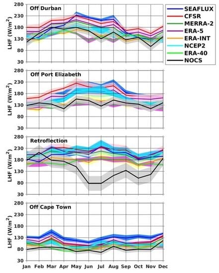
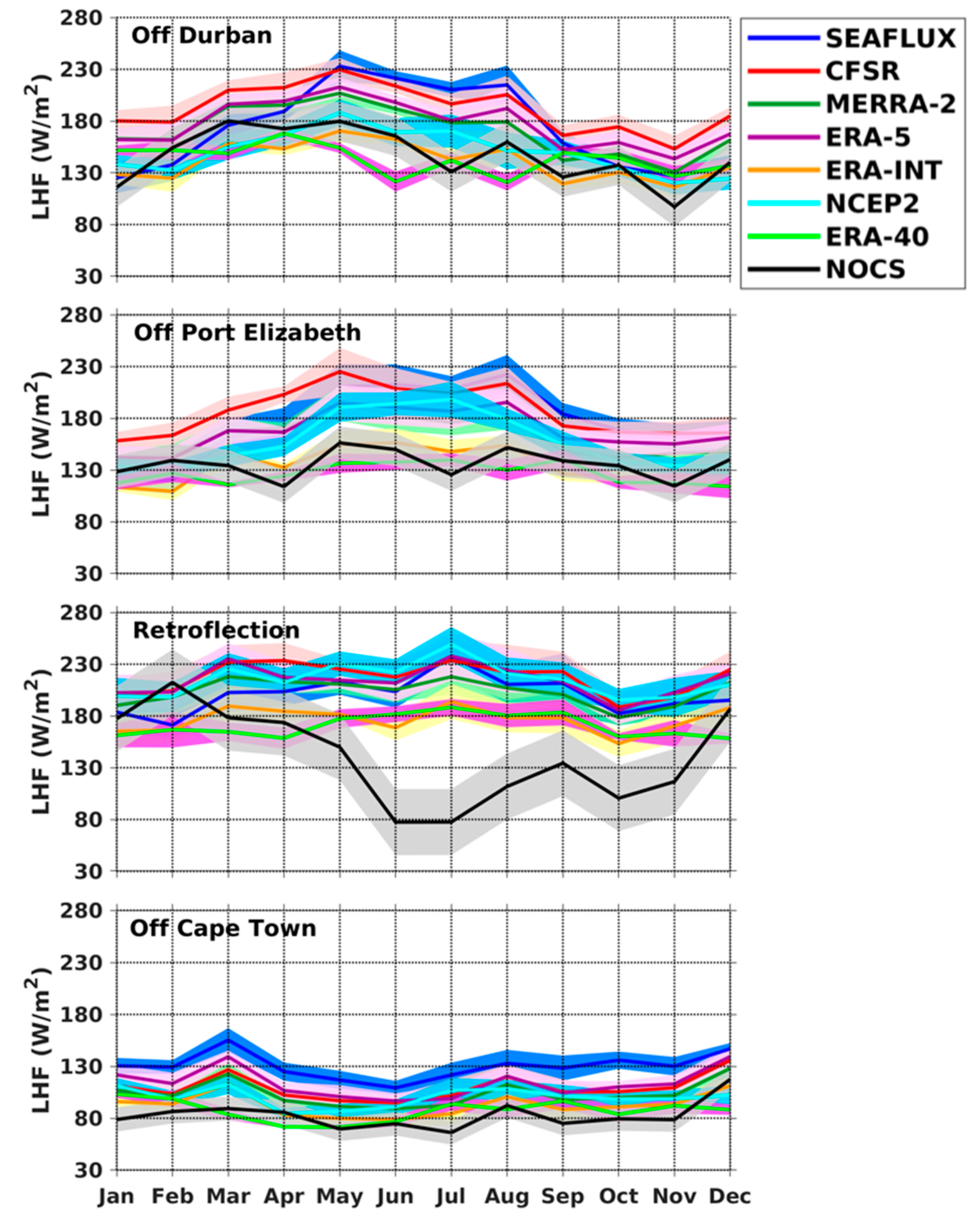
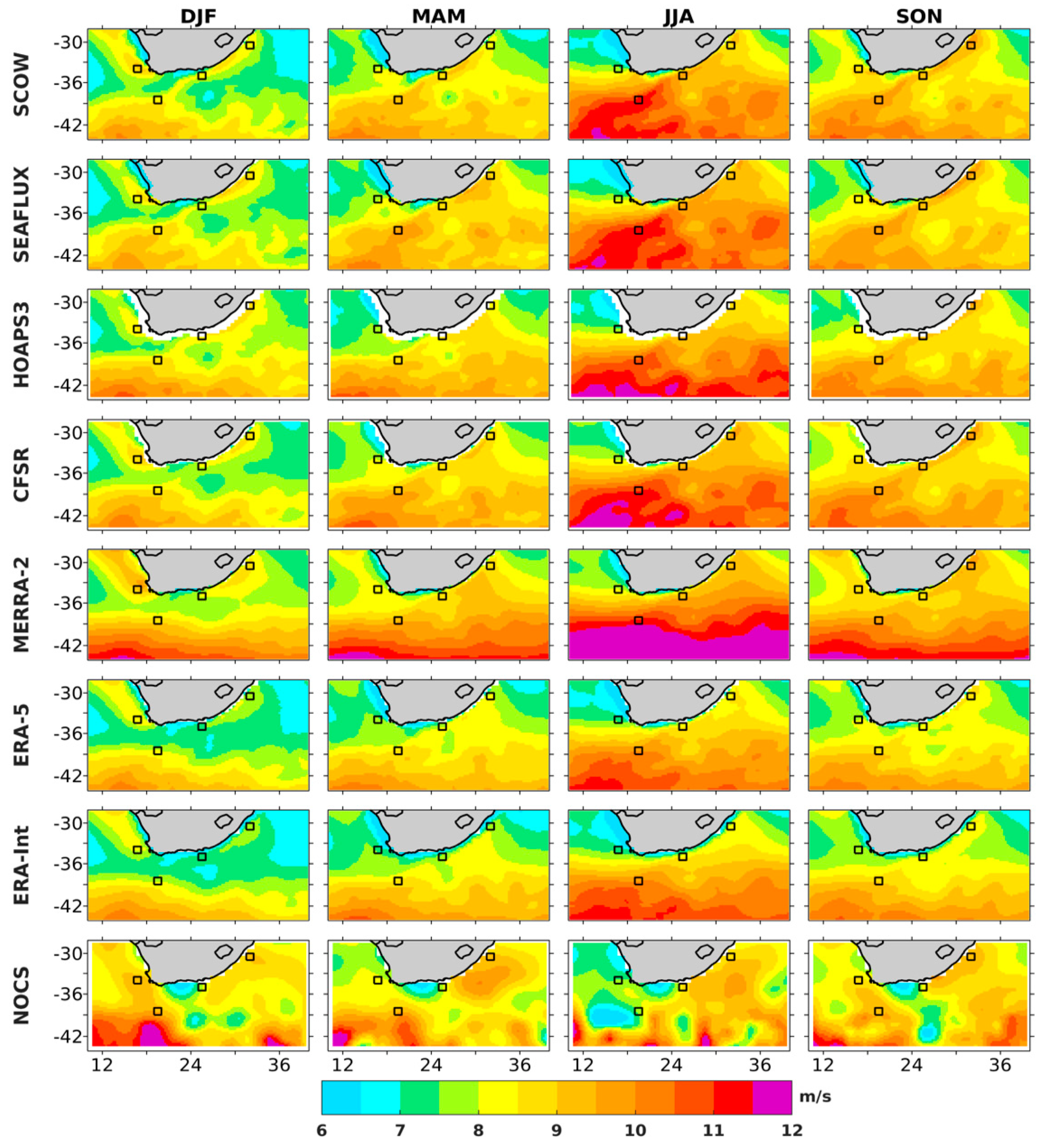
3.1. Seasonal Mean and Annual Cycle of Latent Heat Flux

The seasonal LHF averages derived from the different products (presented in Table 1) are shown in Figure 2 for the Austral summer (December to February—DJF); autumn (March to May—MAM); winter (June to August—JJA) and spring (September to November—SON). In the Agulhas Current system, the LHF ranges from about 100 to 250 W/m2 with maxima during austral autumn and winter depending on the product. In comparison, the minimum LHF of about 50 W/m2 is found during austral summer in the Benguela upwelling region. Towards the colder Southern Ocean, the LHF is also low (around 50 W/m2) for all seasons. We notice that the spatial pattern of the LHF for the austral winter season (JJA) is in good agreement with the MODIS SST field shown in Figure 1.
The large-scale patterns in the seasonal cycle of the LHF for the HOAPS3 and SEAFLUX satellite-based estimates, and the high-resolution CFSR, MERRA-2, and ERA-5 reanalyses products are in fairly good agreement. As HOAPS3 is missing data along the coast it cannot represent the LHF in the Benguela upwelling region and along the Agulhas Current east of Port Elizabeth. The ERA-interim and ERA-40 products have similar seasonality but much lower LHF in autumn and winter than the SEAFLUX, HOAPS3, CFSR, MERRA-2 and ERA-5 products. NOCS is quite different with a distinct maximum of ~250 W/m2 in austral summer and a minimum in winter (between 125 and 175 W/m2) above the Agulhas Retroflection region. ERA-40 and NCEP2 do not adequately represent and underestimate the LHF of the Agulhas Current system because they do not have sufficient resolution to represent the Agulhas Current SST as we will see later (see Section 3.3 and Section 3.4). Moreover, ERA-40 and NCEP2 do not reproduce the meandering shape of the Agulhas Return Current.
The annual cycles of all the LHF products, except HOAPS3, are shown in Figure 3 for the four locations off Durban, off Port Elizabeth, in the Retroflection and off Cape Town. HOAPS3 is omitted because of the missing data along the coast. There are differences between the LHF products both in time and space where their standard errors do not overlap. The LHF varies between 40 and 260 W/m2 in the Agulhas system, and between 40 and 175 W/m2 off Cape Town.
There are differences for all data sets in maximum and minimum and in phases and amplitudes. For instance, off Durban, the SEAFLUX maximum is 230 W/m2 in May; the minimum is nearly 130 W/m2 in January. For the other products, the highest LHF values occur between March and June and the lowest values between November and February. SEAFLUX, CFSR, MERRA-2, and ERA-5 overlap. ERA-Interim, NCEP2, ERA-40, and NOCS overlap except in May-June and August where ERA-40 is smaller. All in all, the CFSR has the highest mean annual value (192 W/m2) and ERA-Interim the lowest (141 W/m2) (see Table 2). SEAFLUX, MERRA-2 and ERA-5 agree well.
Off Port Elizabeth the annual cycles are similar (Figure 3). In this region, the SEAFLUX product has a maximum in August and minimum in January. The other products have their maximum values between May and August and minima between September and February. SEAFLUX, CFSR MERRA-2, and ERA-5 overlap. From April to August ERA-Interim, ERA-40, and NOCS do not overlap with the former products. Lowest values in the Agulhas Current system are found off Port Elizabeth in late summer (~100 W/m2).
In the Retroflection area the highest value is found in July for all products except for NOCS which has the lowest value (~80 W/m2) during winter but the highest (210 W/m2) in February. SEAFLUX, CFSR, MERRA-2, ERA-5, ERA-Interim and NCEP2 overlap. NOCS does not overlap with the others for most of the year and its standard error is quite large compared to other products. All in all, CFSR has the highest LHF (217 W/m2) and NOCS the lowest (141 W/m2) (Table 2). Averaging the three Agulhas locations (Table 2) CFSR has the highest LHF; ERA- interim, ERA-40 and NOCS have the lowest LHF.
Off Cape Town, SEAFLUX is higher than any other product (Figure 3 and Table 2). For the whole year, all the products overlap together except for SEAFLUX that overlaps with CFSR and NCEP2 between May and September only.
To summarize, we find that the LHF data sets exhibit roughly similar space and time patterns as found globally by Chou et al. [43]; Smith et al. [44]; Bentamy et al. [45] but with substantial differences in magnitude and phasing of maxima and minima.

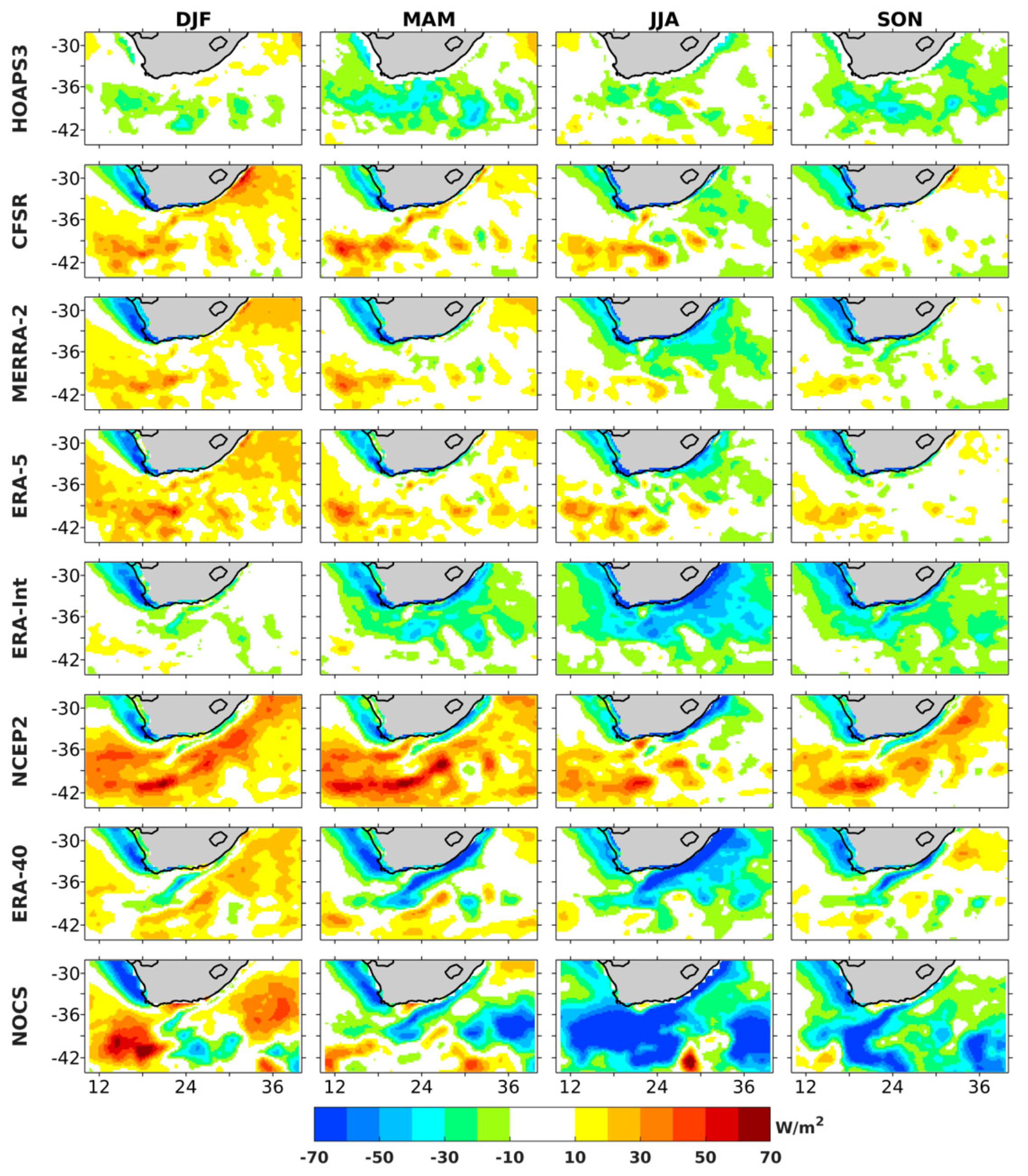
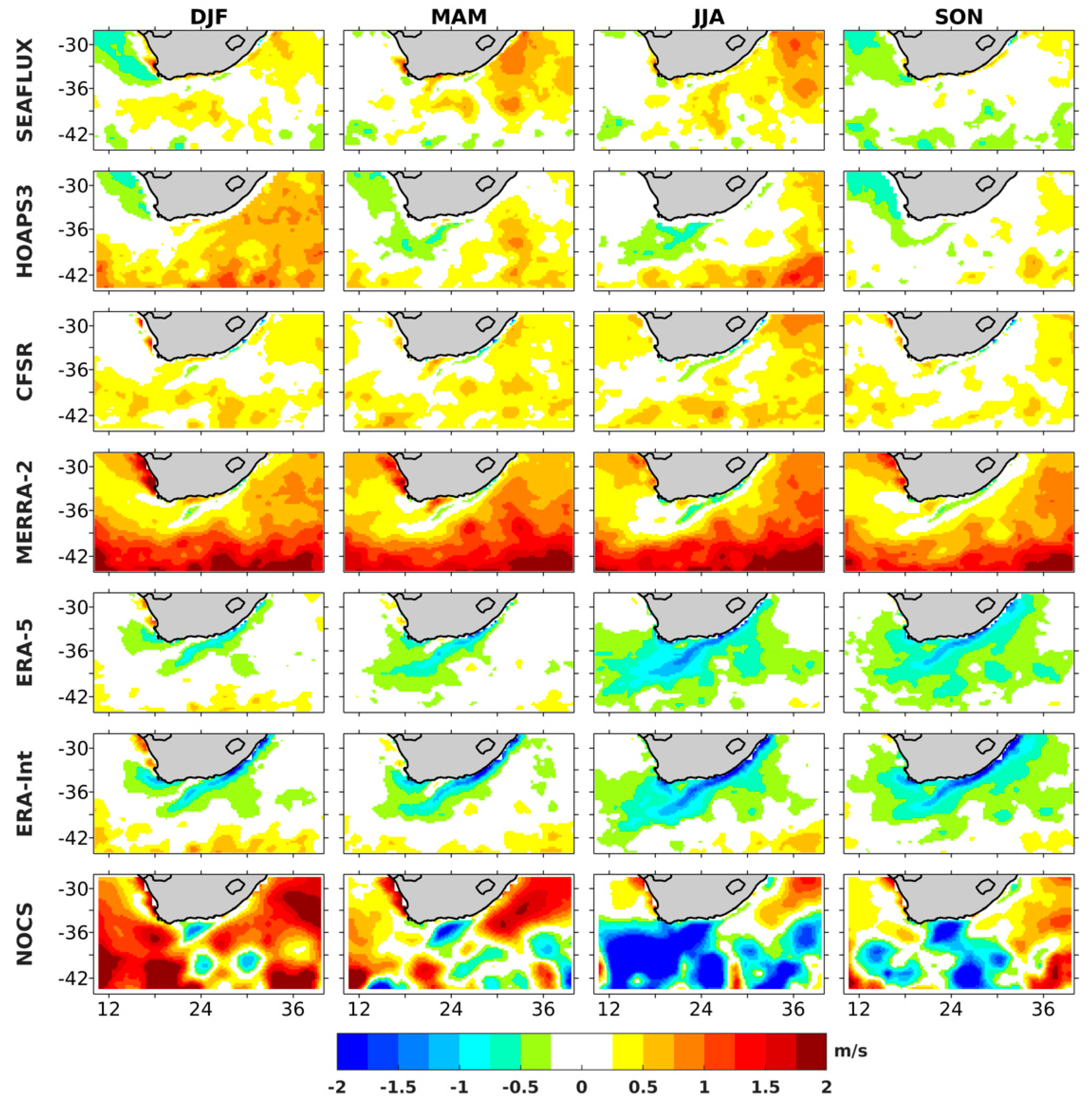
3.2. Differences of Latent Heat Flux between SEAFLUX and Other Products

The mean seasonal differences between the different observation-based and reanalyses-based LHF and SEAFLUX are shown in Figure 4. The LHF products have been interpolated on the grid of SEAFLUX. The differences range within ±70 W/m2, roughly ±38% of the annual mean value of SEAFLUX LHF for the three Agulhas locations (Table 2). Differences can be positive or negative and sometimes have the shape of the Agulhas Current which indicates the problem of low-resolution SST. HOAPS3 is around 30 W/m2 lower than SEAFLUX in the Agulhas Return Current for each season. The positive differences between CFSR and SEAFLUX (CFSR–SEAFLUX) are mostly seen in the Agulhas Current system and reach up to 60 W/m2 during summer (DJF). All reanalyses and NOCS underestimate the LHF in the Benguela system by about 70 W/m2. In the Agulhas Current system along the coast during summer, differences between ERA-5 and SEAFLUX are less than with ERA-Interim. NCEP2 and ERA-40 underestimate the LHF along the coast for all seasons, especially during winter with a difference of 60 W/m2. This is due to the low-resolution of their SST field as further addressed in the next section. In summer, NOCS LHF is almost similar to SEAFLUX from off Durban to off Port Elizabeth. During winter, the difference between NOCS and SEAFLUX is less than 70 W/m2. This could indicate that too few Voluntary Observing vessels are taking measurements in the Agulhas Current system. Indeed, vessels have a tendency to leave the Agulhas Current at the location off Port Elizabeth cruising towards Cape Town or they avoid the southwest flowing Agulhas Current as much as possible when sailing towards Durban [19].
In the coming sections the individual contributions of SST, wind speed and specific humidity to the LHF are examined in order to understand the origin of the differences between products.

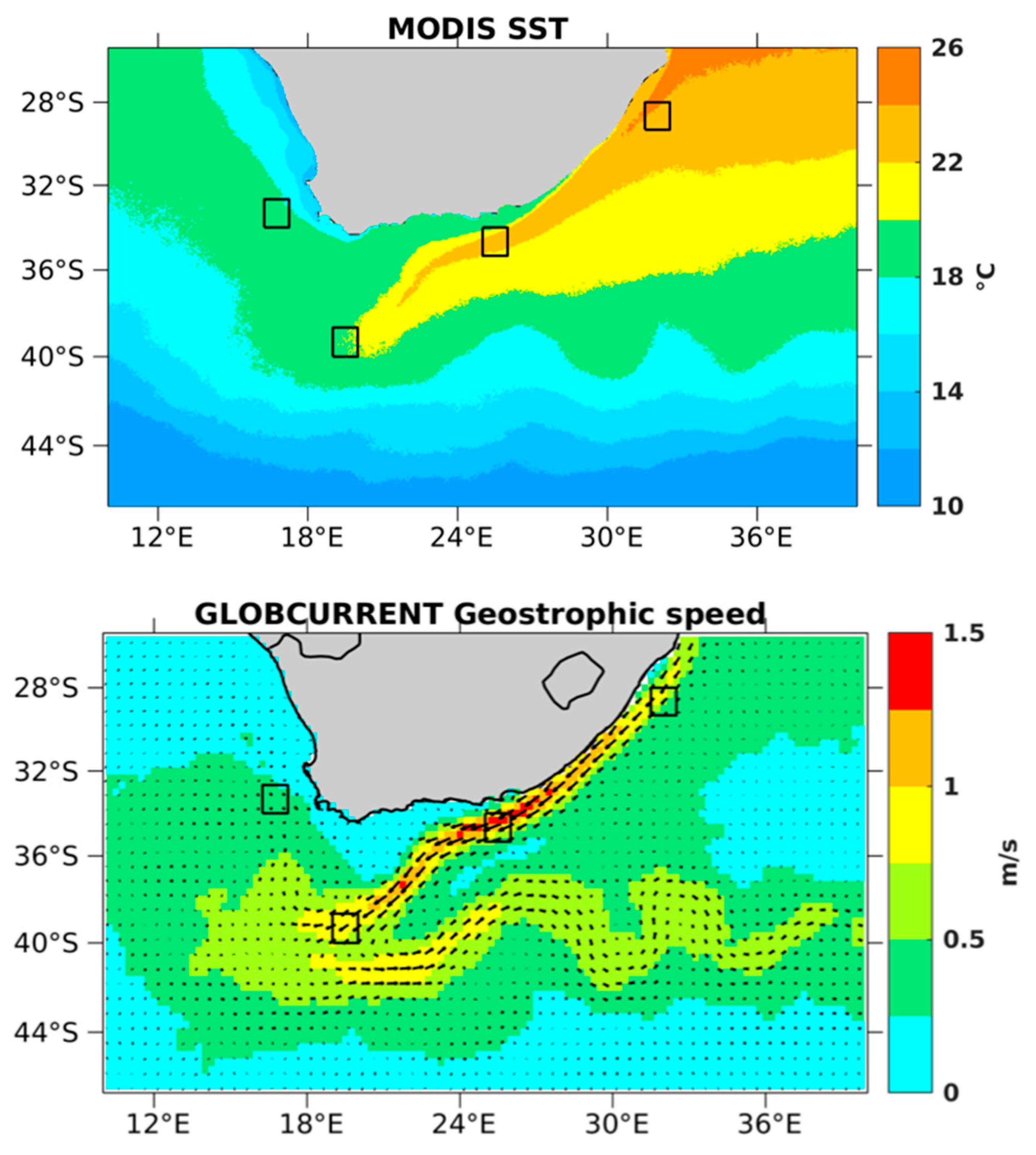
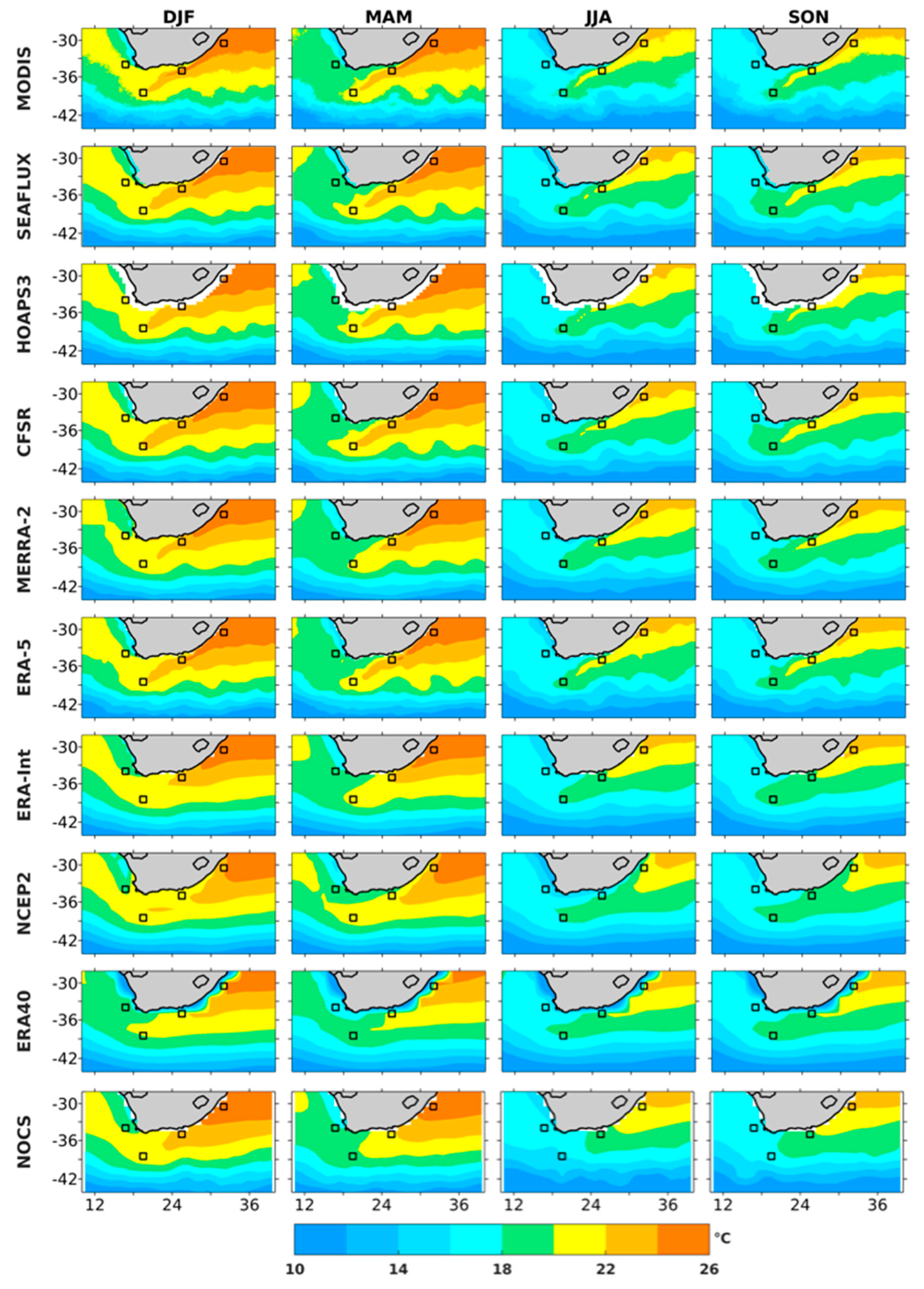
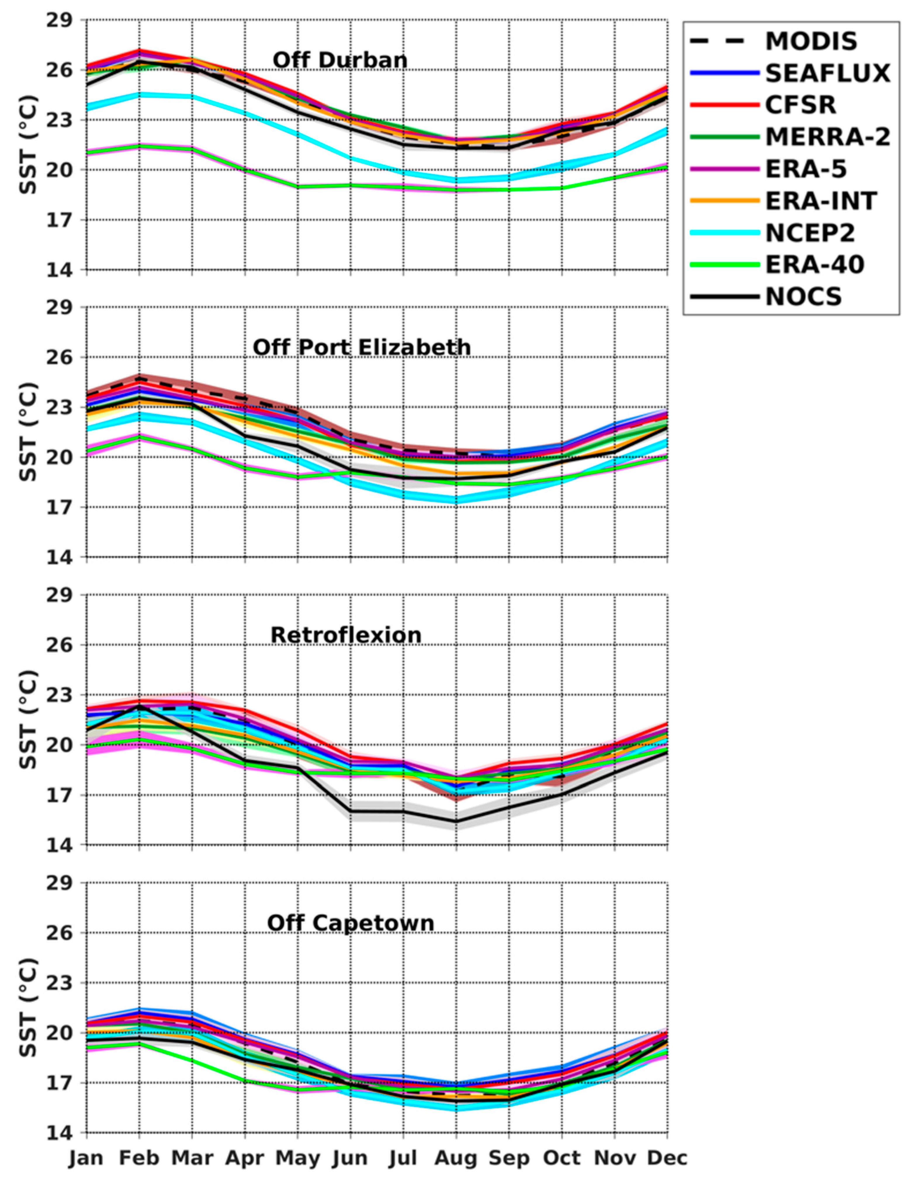
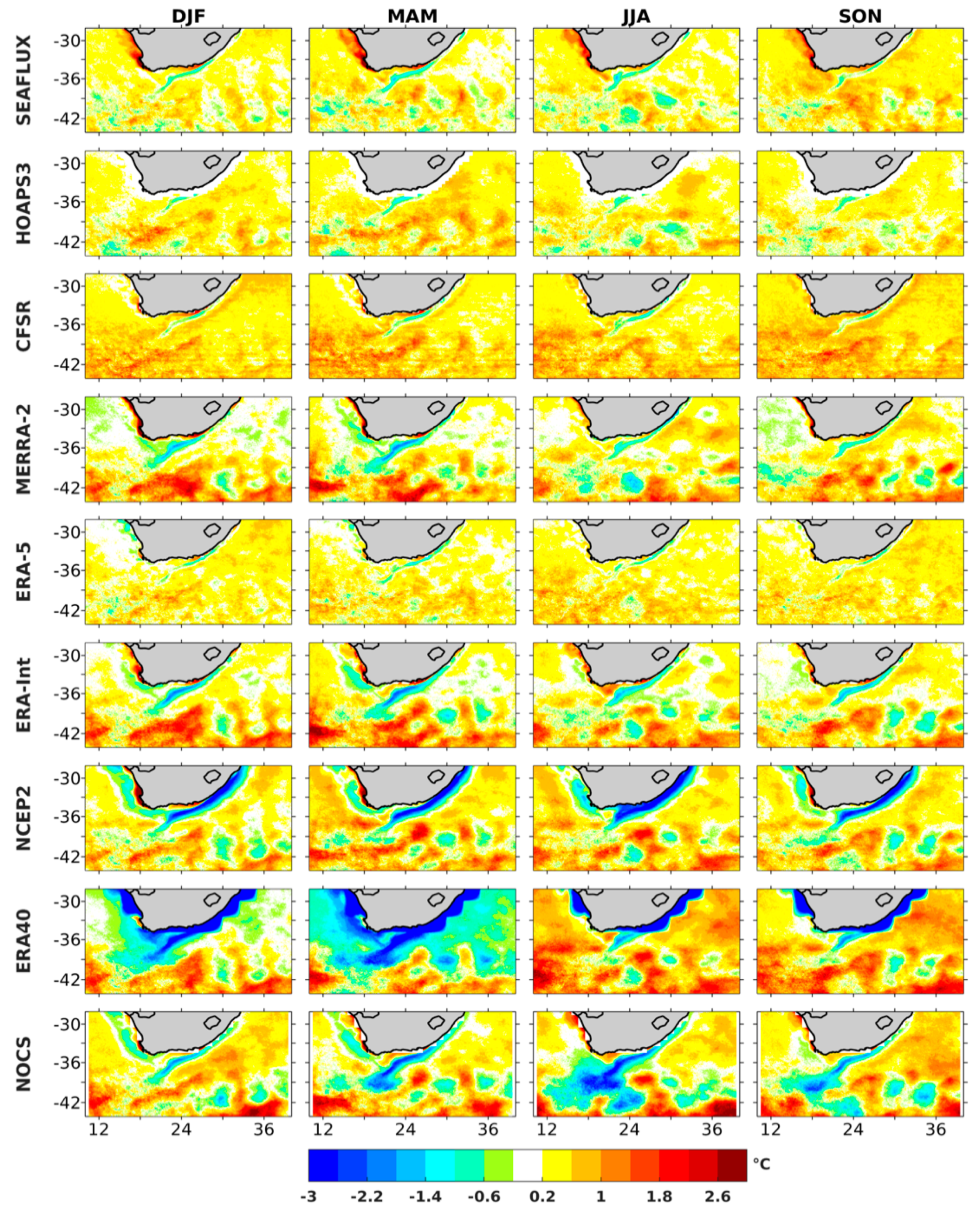
3.3. Seasonal Mean and Annual Cycle of Sea Surface Temperature

The seasonal SST averages derived from the different products (Table 1) are presented in Figure 5 for austral summer, autumn, winter and spring. With its high-resolution (4 × 4 km) MODIS SST is taken as the reference for the comparison of SST. The MODIS SST fields align well with the Agulhas Current velocity structure (Figure 1). In the Agulhas Current system (Figure 5), the SST field ranges from about 18 to 26 °C with the maximum during summer (DJF) and autumn (MAM) and minimum SST in the Retroflection region in winter (JJA).
The large-scale patterns of SST for MODIS, SEAFLUX, and HOAPS3 are similar, but HOAPS3 is missing data along the coast (Figure 5). CFSR, MERRA-2 and ERA-5 have the same horizontal distribution as MODIS. ERA-Interim underestimates the SST in the Agulhas Current. NCEP2 and ERA-40 are around 4°C less than MODIS along the coast. The low-resolution of these reanalyses is clearly apparent as they are not able to adequately resolve the Agulhas Current SST. There is also a poor representation of the meanders of the Agulhas Return Current in SST for NCEP2 and ERA-40. NOCS also underestimates the SST field in the core of the Agulhas Current.
The annual cycles of all SST products (with quite small standard errors) except HOAPS3 are shown in Figure 6 for the four locations of this study. The annual variations of SST are in good agreement with MODIS SST with maxima in late summer and minima in late winter.
Off Durban, MODIS SST ranges between 18 and 28°C. SEAFLUX, CFSR, MERRA-2, ERA-5, ERA-Interim and NOCS are similar to MODIS. NCEP2 and ERA-40 range between 17 and 24 °C and they do not overlap with other products. From the annual mean, NCEP2 and ERA-40 are respectively 2 and 4 °C lower than MODIS (Table 3).
Off Port Elizabeth, MODIS SST varies between 20 and 25°C. In this region SEAFLUX, CFSR, MERRA-2 ERA-5 and ERA-Interim overlap with MODIS. NCEP2, ERA-40 and NOCS underestimate the SST. The annual mean MODIS SST is 22.1 °C (Table 3). NCEP2 and ERA-40 are respectively 2.3 and 2.7 °C colder than MODIS.
For the Retroflection region MODIS SST is between 16 and 23 °C (Figure 6). NOCS SST is underestimated and does not overlap with other products for most months. This could explain the lowest value of NOCS LHF in this region. Other products do overlap except ERA-40. All in all, the mean annual value of MODIS is 19.9 °C, and NOCS is the coolest (18.4 °C).
Off Cape Town, the SST is between 15 and 22 °C. All SSTs overlap except ERA-40 with a smaller amplitude between February and May. The mean MODIS SST is 18.3 °C (Table 3); ERA-40 is 17.5 °C (the coolest).
The mean seasonal differences between observation-based, satellite-based and reanalysis SST and MODIS SST are shown in Figure 7. The SSTs have been interpolated on the grid of MODIS. The differences range within ±3 °C, roughly ±14% of the annual mean MODIS SST in the Agulhas Current system. The spatial discrepancies between the different SST products and the MODIS SST field display the structure of the Agulhas Current that is better resolved in the high-resolution MODIS SST. NCEP2, ERA-40 and NOCS have the lowest SST in the Agulhas Current system. This will increase errors for the calculation of Qss. This can partially explain the lowest values of the LHF in this region for the respective products (Section 2.4). Differences in SST may also be due to the differences between skin and bulk SST as suggested by Chan and Gao [49].

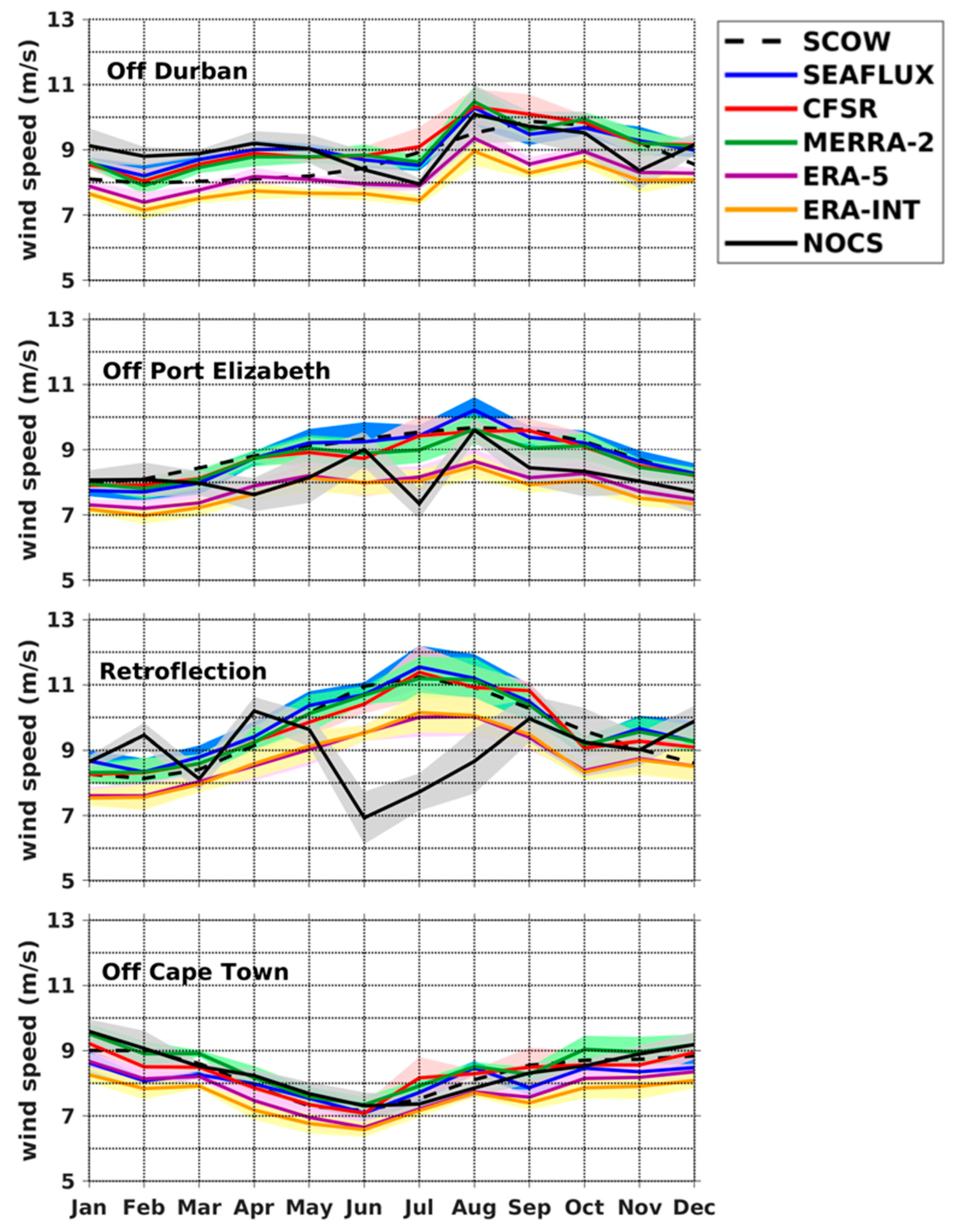
3.4. Seasonal Mean and Annual Cycle of Surface Wind Speed

The seasonal surface wind speed averages from the different products presented in Table 1 are shown in Figure 8 for the austral summer, autumn, winter, and spring. NCEP2 and ERA-40 are not included in the remaining study since their low spatial resolution leads to high errors in SST and LHF in the Agulhas Current system. The satellite-based SCOW product is used as the reference for surface wind speed. The data have been interpolated on the grid of SCOW. SCOW wind speed is clearly stronger above the Agulhas Current than in the surrounding water by about 2 m/s due to the impact of the unstable stratification in the atmospheric boundary layer leading to an increase of the near-surface wind speed across the warm SST front [11]. The wind speed of CFSR, MERRA-2, ERA-Interim and NOCS are re-calculated to equivalent neutral wind using the BVWN algorithm [63], for the convenience of comparing results. For the Agulhas Current system, the maximum wind speed for all products is found in the Retroflection region in austral winter (JJA). We recall that during winter, the LHF reaches its maximum thereof around 250 W/m2 (Figure 2). In comparison, the minimum wind speed is encountered in the Agulhas Current in summer, corresponding to the minimum LHF there.
The large-scale patterns in the seasonal cycle of the wind speed for the SEAFLUX, HOAPS3, CFSR and SCOW products are in fairly good agreement (Figure 8). MERRA-2, ERA-Interim and NOCS misrepresent the meanders of the Agulhas Return Current for each season. In autumn (MAM) and winter (JJA), MERRA-2 overestimates the wind speed in the southern-ocean compared to SCOW. ERA-Interim wind speed is weaker than all other products, and ERA-5 has a stronger wind speed compared to ERA-Interim and it is closer to SCOW. In the Agulhas Current, NOCS maximum is found in austral autumn. In winter, NOCS wind speed appears quite low compared to other products. This is the likely explanation for the low values of the LHF for ERA-Interim and NOCS (around 200 and 150 W/m2 respectively) in the Agulhas Current system.
The annual cycles of near-surface wind speed are represented in Figure 9. The wind speed ranges from 6 to 12 m/s. Off Durban, the wind starts to increase in July with a maximum in August. All the products are in phase, and their amplitudes overlap except for ERA-Interim that is the weakest (Figure 9).
Off Port Elizabeth, the wind has higher seasonal variations compared to Durban. It increases from March until August. This explains why the annual variations of the LHF are more pronounced off Port Elizabeth than off Durban. SEAFLUX is 0.1 m/s lower than SCOW (Table 4). The other products are between 0.2 (MERRA-2, CFSR) and 1.2 m/s (ERA-Interim) lower than SCOW.
The highest values of the annual cycle of wind speed are encountered in the Retroflection region (Figure 8 and Figure 9, Table 4). All the products overlap except NOCS between May and August. NOCS has some maxima and minima that drive the maxima and minima of the NOCS LHF in February, June, and September (Figure 3). The annual mean wind speeds (Table 4) in the Agulhas Current show that SEAFLUX is 0.2 m/s higher than SCOW; while the other products are between 0.1 (MERRA-2, ERA-5) and 0.8 m/s (ERA-Interim) lower than SCOW. CFSR is equal to SCOW. Off Cape Town all the products overlap with SCOW. ERA-Interim has the lowest wind speed, this could explain its lowest LHF in this region (Figure 4, Table 2).
To summarize, for the mean Agulhas region, SEAFLUX is 0.1 m/s higher than SCOW, CFSR and MERRA-2 are similar to SCOW, ERA-5, ERA-Interim, and NOCS are respectively 0.8, 1.0 and 0.4 m/s weaker than SCOW.
The mean seasonal differences between the different observation-based and reanalyses-based wind speed products and SCOW are represented in Figure 10. The differences range within ±2 m/s, around ±22% of the mean SCOW wind speed in the Agulhas system. In the Agulhas Current region, HOAPS3, CFSR and MERRA-2 underestimate the wind speed by around 0.5 m/s, compared to SCOW. Meanwhile, ERA-Interim underestimates the wind speed by around 2 m/s particularly in the Agulhas Current system (Figure 8 and Figure 9, Table 4).

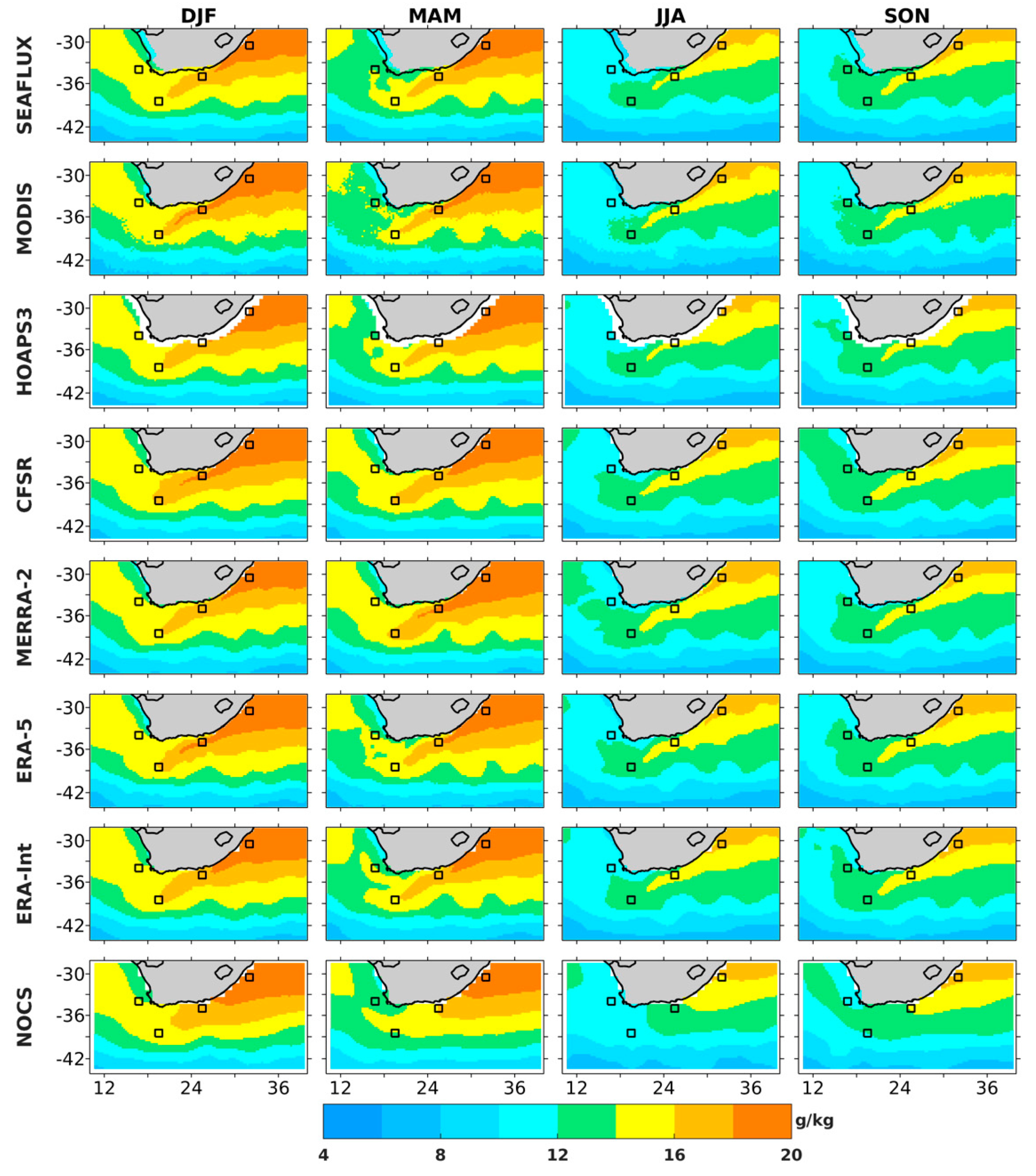
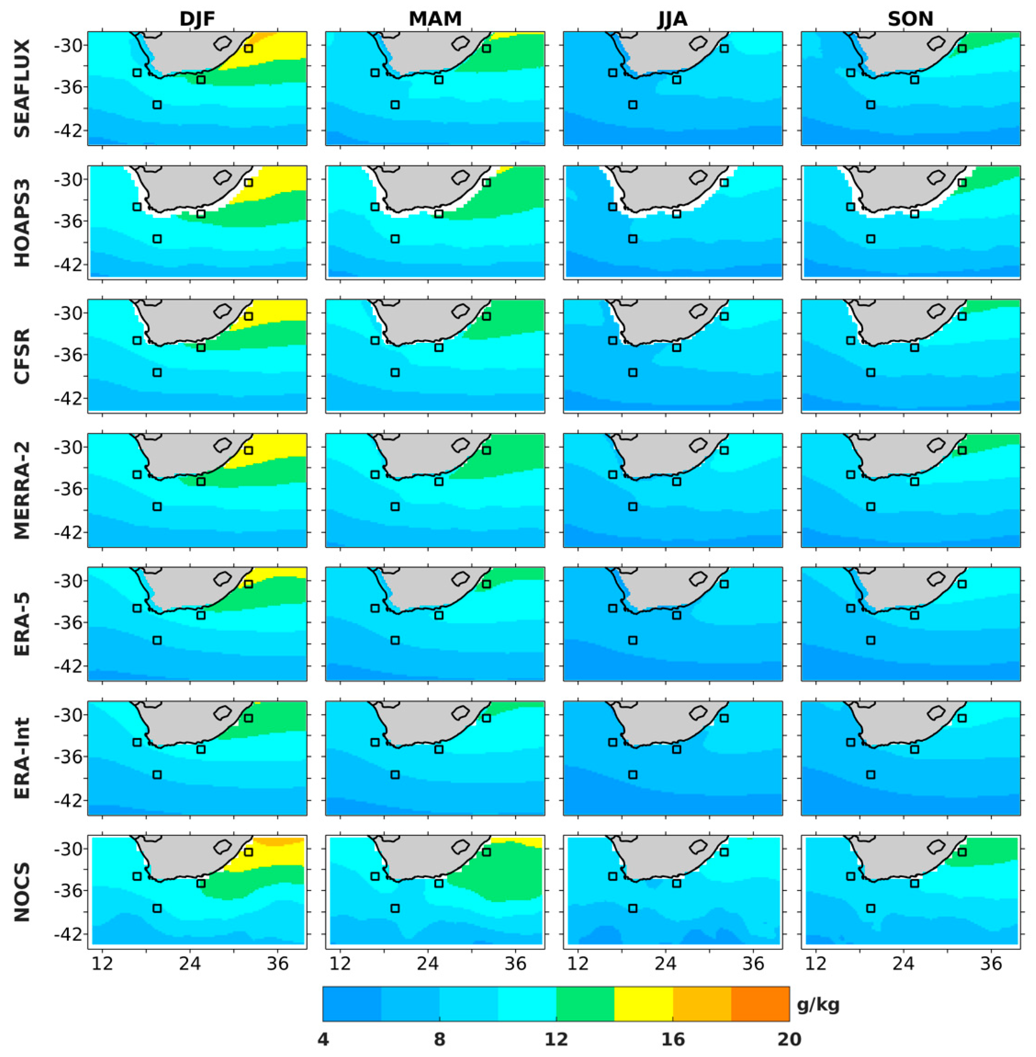
3.5. Seasonal Mean and Annual Cycle of Specific Humidity

3.5.1. Surface Specific Humidity (Qss)

The mean seasonal surface specific humidity (Qss) derived from the different products (presented in Table 1) is shown in Figure 11. ERA-5 and ERA-Interim Qss are computed using their respective SST and the surface pressure, and Equations 1 and 2 of Section 2.3. MODIS Qss is computed using MODIS SST, the surface pressure of ERA-Interim and the Clausius–Clapeyron relation. In the Agulhas Current region, the maximum SEAFLUX Qss ranges from around 16 to 20 g/kg in summer (DJF) and autumn (MAM) and the minimum is between 14 and 18 g/kg in winter (JJA) and spring (SON). As for the SST field, Qss decreases poleward and westward following the pathway of the Agulhas Current. Qss minimum (around 4 g/kg) is observed in the Southern Ocean for all seasons.
The large scale-pattern in the seasonal cycle of the Qss for MODIS, HOAPS3, and ERA-Interim are similar to SEAFLUX Qss. From Port Elizabeth to the Retroflection region, CFSR, MERRA-2, and ERA-5 are in fairly good agreement with SEAFLUX. NOCS fails to capture the sharp maximum in the Agulhas Current and the meanders of the Return Current region

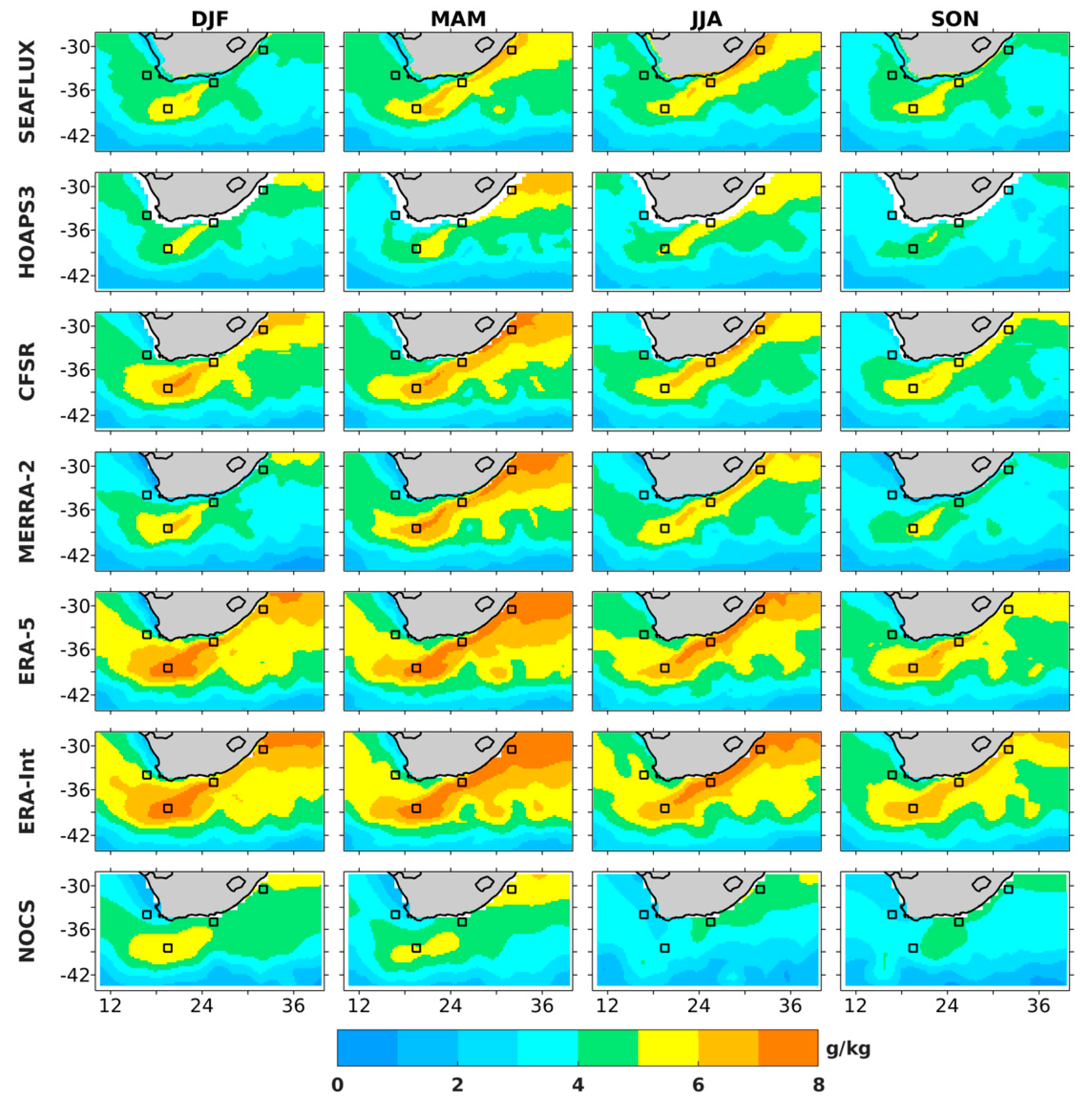
3.5.2. Specific Humidity of Air (Qa)

The specific humidity of the near-surface air (Qa) at a reference height of 10 m is displayed in Figure 12. Qa is available for the products presented in Table 1. The same scale as Qss (Figure 11) is kept for a better comparison. CFSR and ERA-Interim Qa are re-adjusted to 10 m using the BVW algorithm [63]. ERA-5 Qa is available at 10 m. Qa is lower than Qss. The Agulhas Current is not shown as distinctly as it is for the SST, Qss and wind speed. Qa decreases poleward and westward along the pathway of the Agulhas Current like Qss.
The large-scale patterns of CFSR and MERRA-2 are similar compared to the satellite products in summer (DJF) and autumn (MAM). The Qa maximum is found in summer in the eastern part of the Agulhas Current. During winter, the distribution of all products is completely different from one to another, except for ERA-5 and ERA-Interim that look alike. In winter in the Agulhas Current system, Qa ranges between 6 and 12 g/kg for SEAFLUX, HOAPS3, CFSR, MERRA-2 and NOCS, while ERA-5 and ERA-Interim Qa ranges between 6 and 10 g/kg. ERA-5 and ERA-Interim have the lowest Qa product for all seasons which would decrease ERA-Interim LHF and compensate for its low wind speed in the calculation of LHF (Section 2.4).

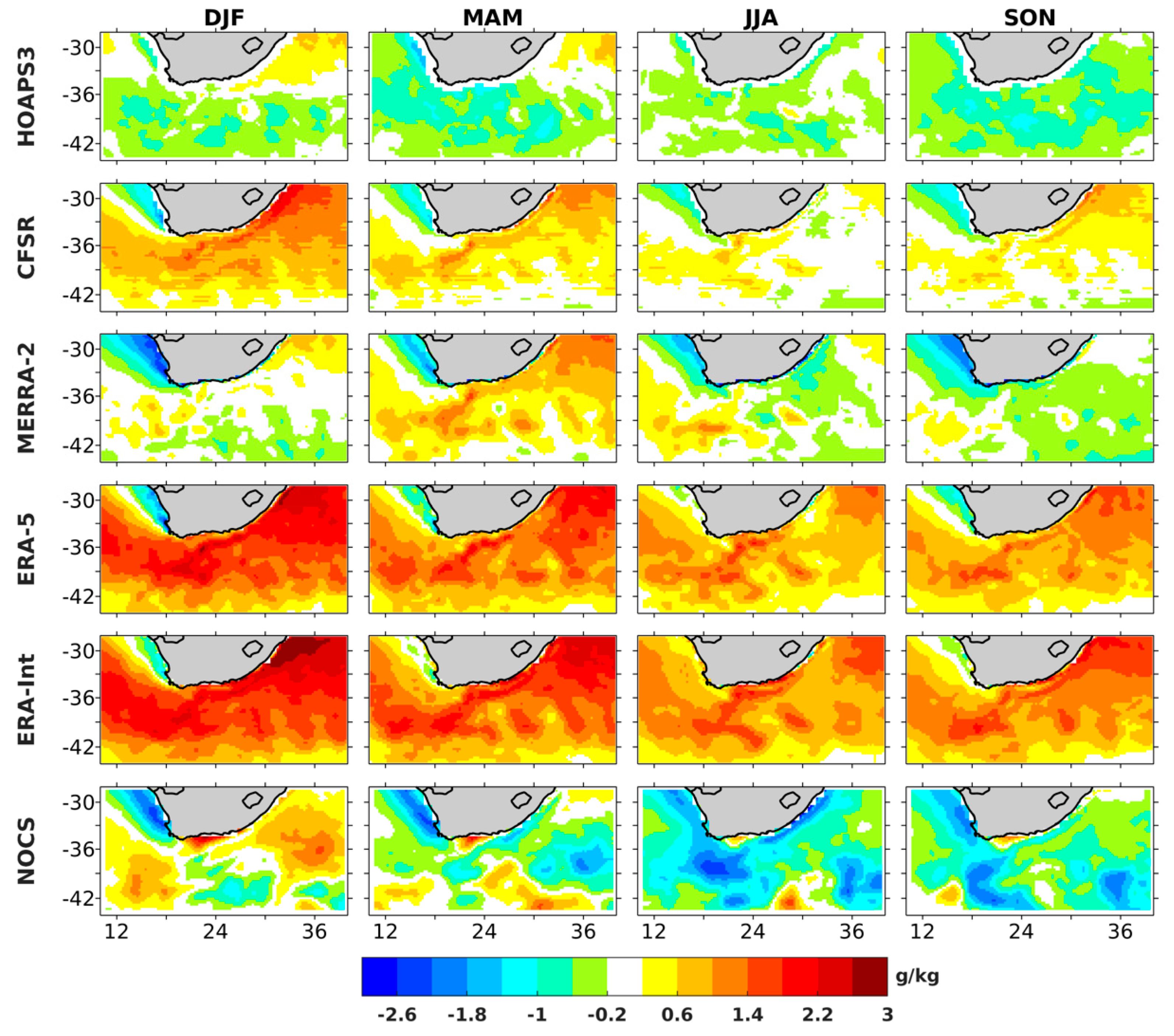
3.5.3. Differences between Surface and Air Specific Humidity (Qss-Qa)

The seasonal differences between sea surface specific humidity and specific humidity of near-surface air (Qss-Qa) for all products are illustrated in Figure 13. According to the bulk formulae in Equation 3 Qss-Qa is as important as the near-surface wind speed to calculate the LHF. Qss-Qa ranges between 0 and 8 g/kg which is equivalent in the calculation of LHF to a wind speed of 0 to 8 m/s. Positives values of Qss-Qa imply evaporation in our study. In the Agulhas Current system Qss-Qa ranges from 4 to 8 g/kg. In spite of uncertainties in the Qa, the spatial pattern of the Agulhas Current is relatively well depicted due to Qss.
The satellite-based HOAPS3, the reanalyses CFSR, MERRA-2, ERA-5 and ERA-Interim have their maximum Qss-Qa in autumn (MAM) and winter (JJA) as for SEAFLUX, but the large scale-patterns do not completely agree with SEAFLUX. NOCS has the lowest Qss-Qa with a minimum in the Agulhas Current in winter. ERA-Interim has the highest Qss-Qa followed by ERA-5, CFSR and MERRA-2.
The annual cycles of Qss-Qa for SEAFLUX, CFSR, MERRA-2, ERA-5, ERA-Interim, and NOCS are displayed in Figure 14 for the four locations of this study. There are considerable differences between the products, but ERA-5 and ERA-Interim have almost the same amplitude. The maxima are located off Durban, with values ranging from 3 to 9 g/kg. The SEAFLUX Qss-Qa maximum is up to 7 g/kg between May and July and decreases thereafter to 3.8 g/kg until mid-spring. SEAFLUX overlaps with CFSR and MERRA-2 from May to August. SEAFLUX, MERRA-2 and NOCS overlap in summer and spring. ERA-Interim has the largest Qss-Qa and overlap with ERA-5 (Figure 14, Table 5).
Off Port Elizabeth the annual cycles of Qss-Qa range between 4 and 8 g/kg. All products have a maximum in March. From May to October, SEAFLUX, CFSR, and MERRA-2 overlap. ERA-5 and ERA-Interim are the highest and NOCS the lowest (Figure 14, Table 5).
In the Retroflection region, Qss-Qa is between 3 and 9 g/kg. SEAFLUX has little annual variations (between 5.5 and 6 g/kg) compared to other products. SEAFLUX overlaps with CFSR and MERRA-2 from June to November. As off Durban and off Port Elizabeth, ERA-5 and ERA-Interim are the largest, and NOCS the smallest. These former products do not overlap with others. NOCS has a maximum (6 g/kg) in February and a minimum in July (~3 g/kg), corresponding to the maximum and minimum of NOCS LHF. In the Retroflection area, the reanalyses are higher than the satellite-based SEAFLUX (Figure 13 and Figure 14, Table 5).
Offshore Cape Town, Qss-Qa ranges from 2 to 5 g/kg (Figure 1). In summary, ERA-5 and ERA-Interim have the largest Qss-Qa values while NOCS reveals the lowest values as seen in Table 5.
The mean seasonal differences of Qss-Qa between HOAPS3, CFSR, MERRA-2, ERA-5, ERA-Interim, NOCS and SEAFLUX product are presented in Figure 15. The differences range within ±2 g/kg, around ±37% of the mean SEAFLUX Qss-Qa in the Agulhas system. In this region, HOAPS3, CFSR, and MERRA-2 overestimate the Qss-Qa by around 2 g/kg compared to SEAFLUX in summer (DJF) and autumn (MAM), but underestimate Qss-Qa by around 1 g/kg in winter (JJA). ERA-5 and ERA-Interim overestimate the Qss-Qa for all seasons (Figure 13 and Figure 15, Table 5), while NOCS overestimates the Qss-Qa in summer and underestimates the Qss-Qa by 2 g/kg in winter.
The second aim of this study was to identify the level of uncertainties introduced by the basic parameters (SST, wind, surface specific humidity) used to estimate the LHF (e.g., Equation (3)). The differences between each product and the reference products from MODIS are calculated for SST, SCOW for wind speed and SEAFLUX for Qss-Qa. CFSR SST is higher than MERRA-2 SST compared to MODIS SST. This may explain higher values of the LHF from CFSR compared to MERRA-2, as SST is used to compute Qss. For a better comparison of the wind speed and Qa between products, we convert the stability-dependant wind speed of CFSR, MERRA-2, ERA-Interim and NOCS to the equivalent neutral wind speed using the BVWN algorithm [63]. The difference between the real wind speed and the re-calculated wind speed is up to 0.5 m/s maximum. We also re-adjust the 2 m Qa to 10 m Qa using the BVW algorithm, for CFSR and ERA-Interim. This correction removes between 0.3 and 0.8 g/kg to the initial 2 m Qa. Between all the new reanalyses, MERRA-2 has the highest wind speed and CFSR the highest Qss-Qa as provided in Table 4 and Table 5. ERA-Interim has the weakest wind speed in the Agulhas system compared to SCOW (Figure 9, Table 4), despite the fact that ERA-Interim wind speed is recalculated using the BVWN algorithm. This explains the lowest values of the ERA-Interim LHF. In the Agulhas Current system, CFSR and MERRA-2 wind speed are similar. ERA-Interim has the strongest Qss-Qa compared to other reanalyses (Figure 14, Table 5). This compensates for the low wind speed in the calculation of ERA-Interim LHF but not enough. Qss-Qa variability is mostly influenced by the variation of Qa. The comparison of the nine LHF products by Smith et al. [44] indicates that in many regions, the differences in Qa between the products clearly have a greater impact than the discrepancies in wind speed and ocean surface temperature. The recent study of Bentamy et al. [45] showed that the differences in LHF tend to be strongly related to large differences in surface wind speeds and/or Qa. The differences of LHF can also be explained by the diversity of algorithms; different bulk flux algorithms (e.g., Brunke et al. [66]); different sources of the input meteorological state variables (e.g., Curry et al. [25]); differences in the boundary conditions; and differences in the procedures for in-situ data collection. Differences can, moreover, arise from the averaging methodology to obtain monthly means. For the satellite-based products, the retrievals of air temperature (Tair) and specific humidity (Qair) at the surface continue to be problematic in regions with strong vertical gradients [44]. Another source of specific uncertainties for the reanalyses is incomplete account of the surface current speed. Looking at the annual mean of the Agulhas Current from the GlobCurrent data repository, the surface current speed can be more than 1.5 m/s. During the ACASEX [5], surface current speeds of up to 2 m/s were measured. Thus, neglecting a 2 m/s current speed at a near-surface wind speed of 4 m/s may lead to a 50% error in the LHF estimation.

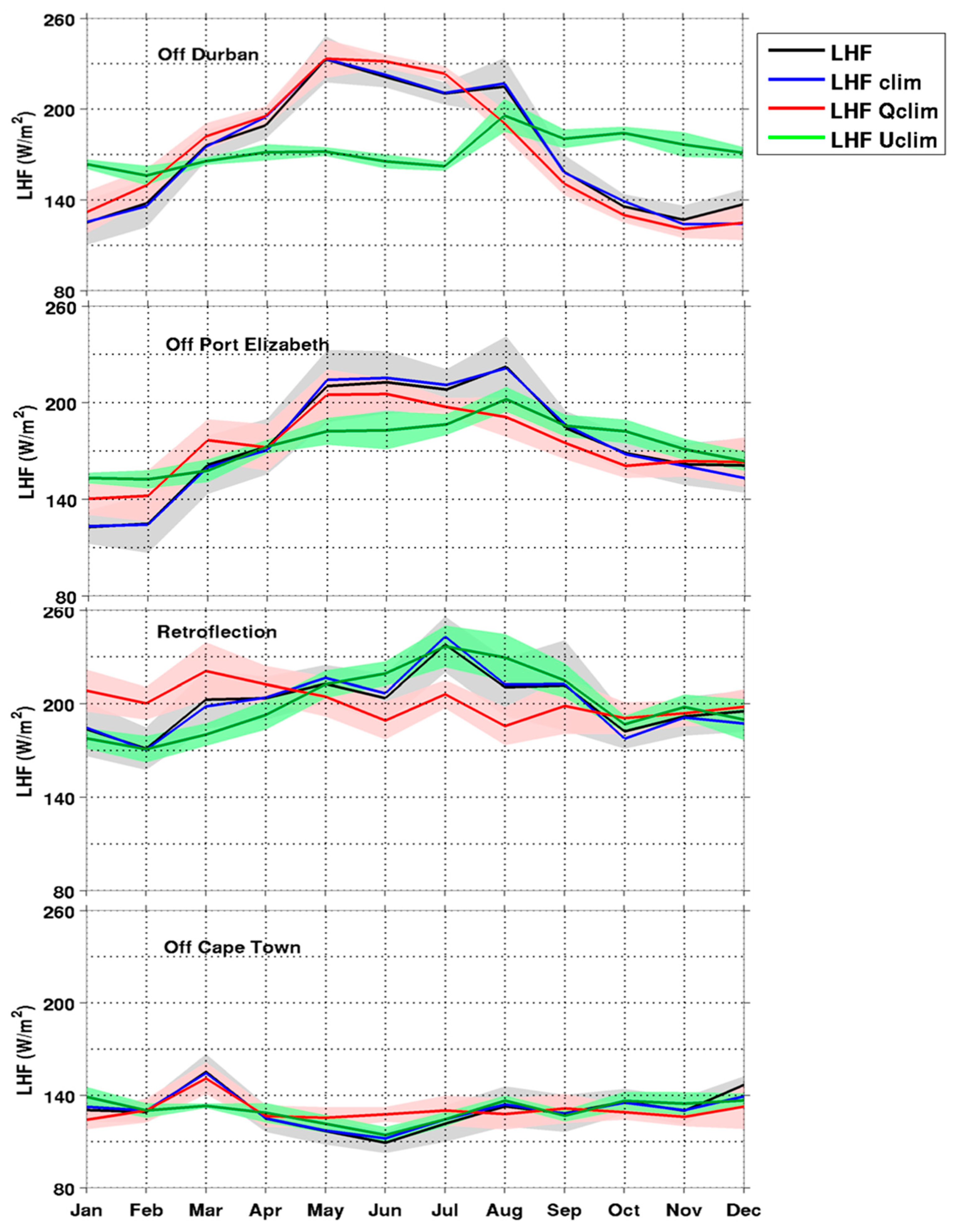
4. Drivers of the Annual Cycle of Latent Heat Flux using SEAFLUX

In this section, the drivers of the annual cycle of the LHF are studied off Durban, Port Elizabeth, Cape Town and in the Retroflection region using SEAFLUX. SEAFLUX is used because SEAFLUX SST agrees rather well with MODIS SST field (Figure 5 and Figure 6), SEAFLUX wind speed also compares well with SCOW wind speed (Figure 8 and Figure 9). SEAFLUX wind speed ranges between 8 and 12 m/s in the Agulhas Current system, and Qss-Qa ranges between 4 and 7 g/kg (Figure 9 and Figure 14). Off Cape Town SEAFLUX wind speed varies between 7 and 9 m/s with Qss-Qa ranging between 4 and 5 g/kg. To evaluate the contribution of either the wind speed or the difference in specific humidity we recalculated 3 types of LHF using the SEAFLUX product (Figure 16) based on Equation (3). LHF calculated with: a) a monthly climatology of wind speed and of Qss-Qa (LHF_clim), b) a monthly climatology of Qss-Qa and the annual mean of wind speed (LHF_Qclim) and c) a monthly climatology of wind speed and the annual mean of Qss-Qa (LHF_Uclim). To recalculate the LHF, we estimate the coefficient ρ a C E l v of Equation (3) as follows:
c o e f = r m s ( L H F ) r m s ( L H F c l i m )
This coefficient is between 3.6 and 3.7, with C E   0.0012 as found by Singh et al. [67]. The authors suggested that C E values range between 0.00152 and 0.00105 for wind speeds between 2 and 19 m/s.
The highest value of the LHF is found in the Retroflection area in winter (around 250 W/m2) while the lowest LHF is off Cape Town (100 W/m2, in winter) (Figure 16). To compare statistically the initial LHF and the recalculated LHF, we show the correlation coefficients, the ratio of variances and the explained variances between LHF and each of the recalculated LHFs (Table 6). The explained variance (EXPvar) is defined as
E X P v a r ( x ) = 100 100 × [ v a r ( L H F L H F x ) v a r ( L H F ) ]
where L H F x is LHF_clim, LHF_Qlim or LHF_Uclim.
The recalculated LHF_clim compares well with the initial LHF for all the locations (Figure 16). The EXPvar is 99% off Durban and off Port Elizabeth, while in the Retroflection region and off Cape Town EXPvar is 95% indicating that LHF_clim represents LHF well even though its amplitude is smaller compared to LHF in these regions. This may be due to the use of monthly means for the correlation. Off Durban, the correlation between LHF and LHF_Qclim is 0.96, and the ratio of variances is 112% with 48% of the EXPvar, while the correlation between LHF and LHF_Uclim is 0.10 with 7% of the ratio of variances (Table 6). This result indicates that off Durban and probably the eastern part of the Agulhas Current is mostly driven by the monthly climatology of Qss-Qa. The monthly climatology of the wind speed only explains 1% of the variance. In the Retroflection region correlation between LHF and LHF_Qclim is 0.13, the ratio of variances is 34% and the EXPvar is 2% while the correlation between LHF and LHF_Uclim is 0.85 with 149% of the ratio of variances and 45% of the EXPvar. This result reveals that in this region and probably the West of the Agulhas Current, the LHF is driven by the monthly climatology of the wind speed rather by the Qss-Qa. Off Port Elizabeth and off Cape Town, the correlation between LHF and LHF_Qclim as well as LHF_Uclim is more than 0.71, statistically significant at the 95% level. This result shows that the LHF is driven by the wind speed and differences in specific humidity for both regions.
To confirm our result, we compared LHF and wind speed on a shorter 5-day average time scale. We represent the annual cycle of the 5-day averages climatology for LHF and wind speed, from 2003 to 2007. We then calculate the correlation between these two parameters in the four regions selected for our study (Figure S3). We notice that the correlation is higher off Port Elizabeth (r = 0.87), in the Retroflection region (r = 0.80) and off Cape Town (r = 0.74). Correlation are significant at the 99%. Off Durban, in contrast, the correlation is low (r = 0.23) and barely significant at the 95%. Therefore, the wind speed cannot be the main driver of the amplitude of the annual cycle of LHF off Durban. This result is in agreement with our findings at a seasonal time scale. We were not able to recalculate the flux using the 5-day averages because of the unavailability of SEAFLUX specific humidity at the sea surface. This represent a limitation of our study.

5. Discussion and Conclusions

In this paper, the first objective was to investigate whether the recent climate reanalyses (CFSR, MERRA-2, ERA-5, ERA-Interim), satellite-based (SEAFLUX, HOAPS3) and in-situ observation-based (NOCS) LHF products have a good representation of the intense turbulent flux of moisture that occurs above the Agulhas Current. This was assessed by comparison to older reanalyses (ERA-40 and NCEP2), since the Agulhas Current is not adequately resolved in these coarser-resolution products. HOAPS3 compares quite well with SEAFLUX, in contrast, HOAPS3 does not have data along the coast. Compared to the SEAFLUX LHF, the ERA-40 and NCEP2 LHF expectedly fail to represent the structure of the Agulhas Current (Figure 2 and Figure 4). Rouault et al. [16] showed that models tend to underestimate the LHF if they are unable to adequately represent the air–sea fluxes over the warmest waters in the Agulhas Current system due to low SST resolution. The new reanalysis products, on the other hand, have a better representation of the current, therefore, are able to adequately represent the LHF in the Agulhas Current system, except ERA-Interim that underestimates the fluxes. However, there are still some difference in the range of LHF value and standard deviation between product, even at the seasonal climatological scale. Differences could arise from the linear interpolation method [68]. Bentamy et al. [44] also proved that the interpolated values tend to be underestimated compared to the original data. The authors compared some global oceans data on 3rd of January 2000. They concluded that the original and interpolated LHF are comparable for most of the variable. The best agreement is for interpolated data estimated from products available with 0.25° grid. Therefore, users must choose a flux product that adequately resolve the features of interest in their research.
The recent study of Parker [69] shows that reanalyses are closer to observations even though they have limitations due to observational constraints and the accuracy of the assimilation in reanalyses. CFSR is relatively similar to MERRA-2 and ERA-5 but has higher LHF. Between the four new reanalyses, surprisingly ERA-Interim has the lowest fluxes (100–200 W/m2). This result was unexpected in view of the higher spatial resolution of the ERA-Interim (0.75° × 0.75°) compared to ERA-40 (2.5° × 2.5°). It is most likely due to its low wind speed although the LHF is compensated by high values of Qss-Qa due to lower SST in ERA-Interim leading to lower Qss. The improved version of ERA-Interim (ERA-5) represent better the LHF in the Agulhas region. The phase of the seasonal cycle of NOCS LHF is reversed in the Retroflection region compared to other products. This might indicate that not enough vessels pass through the Agulhas Retroflection region. Another reason for the uncertainties in NOCS is due to measurement uncertainty [27]. At last looking at the bulk formulae and it is clear that uncertainty and difference between LHF products are equally due to uncertainty in wind speed and Qa. Qss depends on SST therefore on the resolution of the SST product used but it seems that the new reanalysis SST are adequate in the Agulhas Current. It should then be worthwhile to integrate the Agulhas Current speed in further reanalysis to improve the real wind speed and the LHF reanalysed. To conclude, CFSR, MERRA-2 and ERA-5 show good representation of the Agulhas Current LHF and will be used for further analysis to investigate the relation between the intense flux of moisture over the Agulhas Current and the weather and climate in Southern Africa, and to validate mesoscale atmospheric models such as the Weather Research and Forecasting model (WRF [7]). HOAPS3 does not represent the Agulhas Current along the coast, or the Benguela upwelling system adequately.
Finally, the annual cycle of the LHF and its drivers in the Agulhas Current system is investigated using SEAFLUX. SEAFLUX is used to recalculate the LHF using a climatology Qss-Qa and/or wind speed, as it has a high spatial resolution (0.25° × 0.25°) and reliable SST and wind speed. Three locations, representative of various regions of the Agulhas Current system (off Durban, off Port Elizabeth and Retroflection) and one point outside the Agulhas system (off Cape Town) were selected for the comparison. In the Agulhas Current system, the lowest LHF of 100 W/m2 is found off Port Elizabeth in late summer. In contrast, the largest LHF of ~250 W/m2 is located in the Retroflection region in winter. This is consistent with the analysis of Rouault et al. [14] who showed that large LHF from the Agulhas Current and the Retroflection region occur throughout the year but particularly during winter. Our result is also consistent with Liu et al. [69] who showed that large LHF in the Agulhas Retroflection region are due to stronger local wind speed. In this region, large values of LHF are due to stronger wind speed in the Retroflection area. To summarize, off Durban, LHF is mostly driven by the surface specific humidity. In comparison, the LHF is mostly driven by the wind speed in the Retroflection region while it is a combination of specific humidity and wind speed off Port Elisabeth.
At last we hope that this study will help to install a decent air–sea interaction measuring system using eddy correlation on a vessel that does back and forth trip between Port Elizabeth and Durban to get decent measurement of LHF in the Agulhas Current. This could be complemented by Satellite remote sensing estimate of ocean current.

Supplementary Materials

The following are available online at https://www.mdpi.com/2072-4292/11/13/1576/s1, Figure S1: Mean seasonal differences of wind speed (m/s) between Equivalent Neutral wind speed and real wind speed calculated using the BVW height adjustment code, for CFSR, MERRA2, ERA-Interim and NOCS products. From left to right Austral summer (DJF), austral autumn (MAM), austral winter (JJA) and austral spring (SON). Equivalent Neutral wind speed is between 0.1 and 0.5 m/s more than the recalculated real wind speed. Figure S2: Mean seasonal differences of Qa (g/kg) between Qa at 2 m and Qa at 10 m calculated using the BVW height adjustment code for CFSR and ERA-Interim product. From left to right Austral summer (DJF), austral autumn (MAM), austral winter (JJA) and austral spring (SON). Qa at 2 m is between 0.3 and 0.8 more than the recalculated Qa at 10 m. Figure S3: SEAFLUX 5-day average climatology of latent heat flux (blue) and wind speed (wind speed) from 2003 to 2007, off Durban, off Port Elizabeth, Retroflection region, and off Cape Town, with their respective correlations.

Author Contributions

A.S.I.N.N. has analysed the data and drafted the work. M.R. and J.A.J. have contributed to the interpretation of the data and have revised the paper. All the authors have contributed substantially to the work.

Funding

This research received no external funding.

Acknowledgments

The authors express their gratitude to the University of Cape Town, the National Research Foundation SARCHi chair on Ocean-Atmosphere Modeling, WRC, ACCESS, DAAD, the Nansen Tutu Centre for Marine Environmental Research, the SANCOOP SCAMPI NRF project and the GlobCurrent DUE project (AO/1-7472/13/I-LG) for supporting this study. The authors thank Professor Mark A. Bourassa from the Florida State University for helping with the Bourassa–Vincent–Wood Algorithm. The data used for this study are publicly available on http://www.hoaps.org/, http://rda.ucar.edu/, http://www.globcurrent.org, http://apps.ecmwf.int, http://SEAFLUX.org, ftp://podaac.jpl.nasa.gov/OceanTemperature, https://cds.climate.copernicus.eu/cdsapp#!/home, http://cioss.coas.oregonstate.edu/scow/, and http://disc.sci.gsfc.nasa.gov/uui/search/MERRA-2.

Conflicts of Interest

The authors declare no conflict of interest.

References

  1. Beal, L.M.; Elipot, S.; Houk, A.; Leber, G.M. Capturing the transport variability of a western boundary jet: Results from the Agulhas Current Time-Series Experiment (ACT). J. Phys. Oceanogr. 2015, 45, 1302–1324. [Google Scholar] [CrossRef]
  2. Lutjeharms, J.R.E.; Van Ballegooyen, R.C. The Retroflection of the Agulhas Current. J. Phys. Oceanogr. 1988, 18, 1570–1583. [Google Scholar] [CrossRef]
  3. Lutjeharms, J.R.E.; Mey, R.D.; Hunter, I.T. Cloud lines over the Agulhas Current. S. Afr. J. Sci. 1986, 82, 635–640. [Google Scholar]
  4. Rouault, M.; Lee-Thorp, A.M.; Ansorge, I.; Lutjeharms, J.R.E. The Agulhas Current Air–sea Exchange Experiment. S. Afr. J. Sci. 1995, 91, 493–496. [Google Scholar]
  5. Rouault, M.; Lee-Thorp, A.M.; Ansorge, I.; Lutjeharms, J.R.E. Observations of the atmospheric boundary layer above the Agulhas Current during along current winds. J. Phys. Oceanogr. 2000, 30, 70–85. [Google Scholar] [CrossRef]
  6. Jury, M.R.; Pathack, B.; Rautenbach, C.D.W.; Vanheerden, J. Drought over South Africa and Indian Ocean SST: statistical and GCM results. Global Atmos. Ocean Syst. 1996, 4, 47–63. [Google Scholar]
  7. Nkwinkwa Njouodo, A.S.N.; Koseki, S.; Keenlyside, N.; Rouault, M. Atmospheric Signature of the Agulhas Current. Geophys. Res. Lett. 2018, 45, 5185–5193. [Google Scholar] [CrossRef]
  8. O’Neill, L.W.; Chelton, D.B.; Esbensen, S.K.; Wentz, F.J. High-Resolution Satellite Measurements of the Atmospheric Boundary Layer Response to SST Variations along the Agulhas Return Current. J. Clim. 2005, 18, 2706–2723. [Google Scholar] [CrossRef]
  9. Rouault, M.; Verley, P.; Backeberg, B. Wind changes above warm Agulhas Current eddies. Ocean Sci. 2016, 12, 495–506. [Google Scholar] [CrossRef] [Green Version]
  10. Krug, M.; Schilperoort, D.; Collard, F.; Hansen, M.W.; Rouault, M. Signature of the Agulhas Current in ASAR derived wind fields. Remote Sens. Environ. 2018, 217, 340–351. [Google Scholar] [CrossRef]
  11. Chelton, D.B.; Schlax, M.G.; Freilich, M.H.; Milliff, R.F. Satellite Measurements Reveal Persistent Small-Scale Features in Ocean Winds. Sci. 2004, 303, 978–983. [Google Scholar] [CrossRef] [PubMed] [Green Version]
  12. Mey, R.D.; Walker, N.D.; Jury, M.R. Surface heat fluxes and marine boundary layer modification in the Agulhas Retroflection region. J. Geophys. Res. Space Phys. 1990, 95, 15997–16015. [Google Scholar] [CrossRef]
  13. Lee-Thorp, A.M.; Rouault, M.; Lutjeharms, J.R.E. Moisture up- take in the boundary layer above the Agulhas Current: A case study. J. Geophys. Res. 1999, 104, 1423–1430. [Google Scholar] [CrossRef]
  14. Rouault, M.; Lee-Thorp, A.M. Fine-time resolution measurements of atmospheric boundary layer properties between Cape Town and Marion Island. S. Afr. Mar. Sci. 1997, 17, 281–296. [Google Scholar] [CrossRef]
  15. Rouault, M.; Lutjeharms, J.R.E. Air–sea exchanges over an Agulhas eddy at the subtropical convergence. Global Atmos. Ocean Syst. 2000, 7, 125–150. [Google Scholar]
  16. Rouault, M.; Reason, C.J.C.; Lutjeharms, R.E.; Beljaars, A. NCEP Reanalysis and ECMWF operational model underestimation of latent and sensible heat fluxes above the Agulhas Current. J. Clim. 2003, 16, 776–782. [Google Scholar] [CrossRef]
  17. Lutjeharms, J.R.E.; Rouault, M. Observations of cloud formation above Agulhas Current intrusions in the South-east Atlantic. S. Afr. J. Sci. 2000, 96, 577–580. [Google Scholar]
  18. Rouault, M.; White, S.A.; Reason, C.J.C.; Lutjeharms, J.R.E.; Jobard, I. Ocean–Atmosphere Interaction in the Agulhas Current Region and a South African Extreme Weather Event. Weather. Forecast. 2002, 17, 655–669. [Google Scholar] [CrossRef]
  19. Rouault, M.; Penven, P.; Pohl, B. Warming in the Agulhas Current system since the 1980’s. Geophys. Res. Lett. 2009, 36, L12602. [Google Scholar] [CrossRef]
  20. Gimeno, L.; Drumond, A.; Nieto, R.; Trigo, R.M.; Stohl, A. On the origin of continental precipitation. Geophys. Res. Lett. 2010, 37. [Google Scholar] [CrossRef]
  21. Uppala, S.M.; Kallberg, P.W.; Simmons, A.J.; Andrae, U.; Da Costa Bechtold, V.; Fiorino, M.; Gibson, J.K.; Haseler, J.; Hernandez, A.; Kelly, G. A.; et al. The ERA-40 re-analysis. Q. J. R. Meteorol. Soc. 2005, 131, 2961–3012. [Google Scholar] [CrossRef]
  22. Kalnay, E.; Kanamitsu, M.; Kistler, R.; Collins, W.; Deaven, D.; Gandin, L.; Iredell, M.; Saha, S.; White, G.; Woollen, J.; et al. The NCEP/NCAR 40-year reanalysis project. Bull. Am. Meteorol. Soc. 1996, 77, 437–471. [Google Scholar] [CrossRef]
  23. Kanamitsu, M.; Ebisuzaki, W.; Woollen, J.; Yang, S.-K.; Hnilo, J.J.; Fiorino, M.; Potterl, G.L. NCEP–DOE AMIP-II Reanalysis (R-2). Bull. Amer. Meteor. Soc. 2002, 83, 1631–1643. [Google Scholar] [CrossRef]
  24. Saha, S.; Moorthi, S.; Pan, H.L.; Wu, X.; Wang, J.; Nadiga, S.; Tripp, P.; Kistler, R.; Woollen, J.; Behringer, D.; et al. The NCEP climate forecast system reanalysis. Bull. Am. Meteorol. Soc. 2010, 91, 1015–1057. [Google Scholar] [CrossRef]
  25. Curry, J.A.; Bentamy, A.; Bourassa, M.A.; Bourras, D.; Bradley, E.F.; Brunke, M.; Castro, S.; Chou, S.H.; Clayson, C.A.; Emery, W.J.; et al. SEAFLUX. Bull. Amer. Meteor. Soc. 2004, 85, 409–424. [Google Scholar] [CrossRef] [Green Version]
  26. Woodruff, S.D.; Slutz, R.J.; Jenne, R.L.; Steurer, P.M. A comprehensive ocean-atmosphere dataset. Bull. Am. Meteorol. Soc. 1987, 68, 1239–1250. [Google Scholar] [CrossRef]
  27. Berry, D.I.; Kent, E.C. A new air–sea interaction gridded dataset from ICOADS with uncertainty estimates. Bull. Am. Meteorol. Soc. 2009, 90, 645–656. [Google Scholar] [CrossRef]
  28. Berry, D.I.; Kent, E.C. Air–sea fluxes from ICOADS: the construction of a new gridded dataset with uncertainty estimates. Intern. J. Climatol. 2011, 31, 987–1001. [Google Scholar] [CrossRef]
  29. Reynolds, R.W.; Smith, T.M. Improved global sea surface temperature analyses using optimum interpolation. J. Clim. 1994, 7, 929–948. [Google Scholar] [CrossRef]
  30. Lornec, A.C. A global three-dimensional multivariate statistical interpolation scheme. Mon. Weather. Rev. 1981, 109, 701–721. [Google Scholar] [CrossRef]
  31. Thomas, B.R.; Kent, E.C.; Swail, V.R.; Berry, D.I. Trends in ship wind speeds adjusted for observation method and height. Intern. J. Climatol. 2008, 28, 747–763. [Google Scholar] [CrossRef]
  32. Smith, S.D. Wind stress and heat flux over the ocean in gale force winds. J. Phys. Oceanogr. 1980, 10, 709–726. [Google Scholar] [CrossRef]
  33. Smith, S.D. Coefficients for sea surface wind stress, heat flux, and wind profiles as a function of wind speed and temperature. J. Geophys. Res. 1988, 93, 15467–15472. [Google Scholar] [CrossRef]
  34. Kent, E.C.; Kaplan, A. Towards estimating climatic trends in SST. Part III: systematic biases. J. Atmos. Oceanic Technol. 2006, 23, 487–500. [Google Scholar] [CrossRef]
  35. Josey, S.A.; Kent, E.C.; Taylor, P.K. New insights into the ocean heat budget closure problem and analysis of the SOC air–sea flux climatology. J. Clim. 1999, 12, 2856–2880. [Google Scholar] [CrossRef]
  36. Clayson, C.A.; Roberts, J.B.; Bogdanoff, A. SEAFLUX Version 1: a new satellitebased ocean-atmosphere turbulent flux dataset. Int. J. Climatol. 2013. submitted. [Google Scholar]
  37. Andersson, A.; Fennig, K.; Klepp, C.; Bakan, S.; Graßl, H.; Schulz, J. The Hamburg Ocean Atmosphere Parameters and Fluxes from Satellite Data HOAPS-3. Earth Syst. Sci. 2010, 2, 215–234. [Google Scholar]
  38. Andersson, A.; Fennig, K.; Klepp, C.; Bakan, S.; Graßl, H.; Schulz, J. Evaluation of HOAPS-3 ocean surface freshwater flux components. J. Appl. Meteorol. Climatol. 2011, 50, 379–398. [Google Scholar] [CrossRef]
  39. Casey, K.S. Global AVHRR 4 km SST for 1985-2001; Pathfinder V5.0, NODC/RSMAS, Technical Report; NOAA National Oceanographic Data Center: Silver Spring, MD, USA, 2004. [Google Scholar]
  40. Murray, F.W. On the Computation of Saturation Vapor Pressure. J. Appl. Meteor. 1967, 6, 203–204. [Google Scholar] [CrossRef]
  41. Bentamy, A.; Katsaros, K.B.; Mestas-Nunez, A.M.; Drennan, W.M.; Forde, E.B.; Roquet, H. Satellite Estimates ofWind Speed and Latent Heat Flux Over the Global Oceans. J. Clim. 2003, 16, 637–656. [Google Scholar] [CrossRef]
  42. Fairall, C.W.; Bradley, E.F.; Hare, J.E.; Grachev, A.A.; Edson, J.B. Bulk parameterization of air–sea fluxes: updates and verification for the COARE algorithm. J. Clim. 2003, 16, 571–591. [Google Scholar] [CrossRef]
  43. Chou, S.H.; Nelkin, E.; Ardizzone, J.; Atlas, J.R. A comparison of latent heat fluxes over global oceans for four flux products. J. Clim. 2004, 17, 3973–3989. [Google Scholar] [CrossRef]
  44. Smith, S.R.; Hughes, P.J.; Bourassa, M.A. A comparison of nine monthly air–sea flux products. International J. Climatol. 2011, 31, 1002–1027. [Google Scholar] [CrossRef]
  45. Bentamy, A.; Piolle, J.-F.; Grouazel, A.; Danielson, R.; Gulev, S.; Frederic, P.; Hamza, A.; Mathieu, P.P.; Von Schuckmann, K.; Sathyendranath, S.; et al. Review and assessment of latent and sensible heat flux accuracy over the global oceans. Remote Sens. Environ. 2017, 201, 196–218. [Google Scholar] [CrossRef] [Green Version]
  46. Reynolds, R.W.; Smith, T.M.; Liu, C.; Chelton, D.B.; Casey, K.S.; Schlax, M.G. Daily high-resolution-blended analyses for sea surface temperature. J. Clim. 2007, 20, 5473–5496. [Google Scholar] [CrossRef]
  47. Roberts, J.B.; Clayson, C.A.; Robertson, F.R.; Jackson, D.L. Predicting near-surface atmospheric variables from Special Sensor Microwave/Imager using neural networks with a first-guess approach. J. Geophys. Res. Atmos. 2010, 115. [Google Scholar] [CrossRef]
  48. Kilpatrick, K.A.; Podestá, G.; Walsh, S.; Williams, E.; Halliwell, V.; Szczodrak, M.; Brown, O.B.; Minnett, P.J.; Evans, R. A decade of sea surface temperature from MODIS. Remote Sens. Environ. 2015, 165, 27–41. [Google Scholar] [CrossRef]
  49. Chan, P.-K.; Gao, B.-C. A comparison of MODIS, NCEP, and TMI sea surface temperature datasets. IEEE Geosci. Remote Sens. Lett. 2005, 2, 270–274. [Google Scholar] [CrossRef]
  50. Rio, M.-H.; Mulet, S.; Picot, N. Beyond GOCE for the ocean circulation estimate: Synergetic use of altimetry, gravimetry, and in situ data provides new insight into geostrophic and Ekman currents. Geophys. Res. Lett. 2014, 41. [Google Scholar] [CrossRef]
  51. Johannessen, J.A.; Chapron, B.; Collard, F.; Rio, M.H.; Piollé, J.F.; Quartly, G.; Shutler, J.; Escola, R.; Donlon, C.; Danielson, R.; et al. GlobCurrent: Sentinel-3 Synergy in action. In Proceedings of the Sentinel-3 for Science Workshop, Venice, Italy, 2–5 June 2015. [Google Scholar]
  52. Hart-Davis, M.; Backeberg, B.C.; Halo, I.E.; Van Sebille, E.; Johannessen, J.A. Assessing the accuracy of satellite derived ocean currents by comparing observed and virtual buoys in the great Agulhas region. Remote Sens. Environ. 2018, 216, 735–746. [Google Scholar] [CrossRef]
  53. Risien, C.M.; Chelton, D.B. A Global Climatology of Surface Wind and Wind Stress Fields from Eight Years of QuikSCAT Scatterometer Data. J. Phys. Oceanogr. 2008, 38, 2379–2413. [Google Scholar] [CrossRef]
  54. Milliff, R.F.; Morzel, J. The global distribution of the time-average wind-stress curl from NSCAT. J. Atmos. Sci. 2001, 58, 109–131. [Google Scholar] [CrossRef]
  55. Bosilovich, M.G.; Lucchesi, R.; Suarez, M. MERRA-2: File Specification. GMAO Office Note No. 9 (Version 1.1); p. 73. Available online: http://gmao.gsfc.nasa.gov/pubs/office_notes (accessed on 8 December 2017).
  56. Hersbach, H.; Dee, D. ERA5 reanalysis is in production. Available online: https://www.ecmwf.int/en/elibrary/16299-newsletter-no-147-spring-2016 (accessed on 24 May 2019).
  57. Dee, D.P.; Uppala, S.M.; Simmons, A.J.; Berrisford, P.; Poli, P.; Kobayashi, S.; Andrae, U.; Balmaseda, M.A.; Balsamo, G.; Bauer, P.; et al. The ERA-Interim reanalysis: Configuration and performance of the data assimilation system. Q. J. Royal Meteorol. Soc. 2011, 137, 553–597. [Google Scholar] [CrossRef]
  58. Griffies, S.M.; Harrison, M.J.; Pacanowski, R.C.; Rosati, A. Technical Guide to MOM4; GFDL Ocean Group Technical Report; NOAA/Geophysical Fluid Dynamics Laboratory: Princeton, NJ, USA, 2004. [Google Scholar]
  59. Rienecker and Coauthors. MERRA - NASA’s Modern-Era Retrospective Analysis for Research and Applications. J. Clim. 2011, 24, 3624–3648. [Google Scholar] [CrossRef]
  60. Taylor, K.E.; Williamson, D.; Zwiers, F. The sea surface temperature and sea-ice concentration boundary conditions for AMIP II simulations; PCMDI Technical Report; Lawrence Livermore National Laboratory, University of California: Livermore, CA, USA, 2000; p. 28. [Google Scholar]
  61. Donlon, C.J.; Martin, M.; Stark, J.; Roberts-Jones, J.; Fiedler, E.; Wimmer, W. The Operational Sea Surface Temperature and Sea Ice Analysis (OSTIA) system. Remote Sens. Environ. 2012, 116, 140–158. [Google Scholar] [CrossRef]
  62. Holm, E.V. Revision of the ECMWF humidity analysis: Construction of a Gaussian control variable. In Proceedings of the ECMWF/GEWEX Workshop on Humidity Analysis, Reading, UK, 8–11 July 2002. [Google Scholar]
  63. Bourassa, M.A.; Vincent, D.G.; Wood, W.L. A flux parameterization including the effects of capillary waves and sea state. J. Atmos. Sci. 1999, 56, 1123–1139. [Google Scholar] [CrossRef]
  64. Bolton, D. Computation of equivalent potential temperature. Mon. Weather. Rev. 1980, 108, 1046–1053. [Google Scholar] [CrossRef]
  65. Buck, A.L. New equations for computing vapor pressure and enhancement factor. J. Appl. Meteorol. 1981, 20, 1527–1532. [Google Scholar] [CrossRef]
  66. Brunke, M.A.; Fairall, C.W.; Zeng, X.; Eymard, L.; Curry, J.A. Which bulk aerodynamic algorithms are least problematic in computing ocean surface turbulent fluxes? J. Clim. 2003, 16, 619–635. [Google Scholar] [CrossRef]
  67. Singh, R.; Joshi, P.C.; Kishtawal, C.M. A new technique for estimation of surface latent heat fluxes using satellites-based observations. Mon. Weather Rev. 2005, 133, 2692–2710. [Google Scholar] [CrossRef]
  68. Sminorv, D.; Newman, M.; Alexander, M.A.; Kwon, Y.O.; Frankignoul, C. Investigating the local atmospheric response to a realistic shift in the Oyashio sea surface temperature front. J. Clim. 2015, 28, 1126–1147. [Google Scholar]
  69. Liu, J.; Xiao, T.; Chen, L. Intercomparisons of air–sea heat fluxes over the Southern Ocean. J. Clim. 2011, 24, 1198–1211. [Google Scholar] [CrossRef]
Figure 1. (Top) Moderate Resolution Imaging Spectroradiometer (MODIS) surface temperature (SST) (°C) annually averaged from 2003 to 2007 and (bottom) GlobCurrent geostrophic current speed (colour) and direction (arrows) at 0 m depth. Black squares represent the four locations of time series used in the study: three regions in the Agulhas system: off Durban (31.5–32.5°E; 30–31°S), off Port Elizabeth (25–26°E; 34.5–35.5°S) and in the Agulhas Retroflection (19–20°E; 38–39°S), and one point off Cape Town (16–17°E; 33.5–34.5°S).
Remotesensing 11 01576 g001
Figure 2. From top to bottom: seasonal average of latent heat flux (W/m2) of SEAFLUX, HOAPS3, CFSR, MERRA-2, ERA-Interim, NCEP2, ERA-40 and NOCS. From left to right austral summer (December to February—DJF), austral autumn (March to May—MAM), austral winter (June to August—JJA), and austral spring (September to November—SON). Black squares represent the four locations taken for the study as in Figure 1, Agulhas Current off Durban, Agulhas Current off Port Elizabeth, Agulhas Retroflection and off Cape Town.
Remotesensing 11 01576 g002
Figure 3. Annual cycles of latent heat flux (W/m2). In Agulhas Current off Durban (31.5–32.5°E; 30–31°S), off Port Elizabeth (25–26°E; 34.5–35.5°S), Agulhas Retroflection (19–20°E; 38–39°S) and off Cape Town (16–17°E; 33.5–34.5°S) for SEAFLUX (blue), CFSR (red), MERRA-2 (green), ERA-5 (purple), ERA-Interim (yellow), NCEP2 (cyan), ERA-40 (purple) and NOCS (black). Shades areas represent the standard errors calculated as the standard deviation divided by the square root of the number of years.
Remotesensing 11 01576 g003
Figure 4. Mean seasonal differences of latent heat flux (W/m2) between the observation-based, the reanalysis products, and SEAFLUX product. From left to right austral summer (DJF), austral autumn (MAM), austral winter (JJA) and austral spring (SON). The products have been interpolated on the grid of SEAFLUX (0.25° × 0.25°).
Remotesensing 11 01576 g004
Figure 5. From top to bottom: seasonal average of sea surface temperature SST (°C) of MODIS, SEAFLUX, HOAPS3, CFSR, MERRA-2, ERA-Interim, NCEP2, ERA-40 and NOCS. From left to right austral summer (DJF), austral autumn (MAM), austral winter (JJA) and austral spring (SON). Black squares represent the four locations taken for the study. MODIS SST is the reference for SST. The products have been interpolated on the grid of MODIS.
Remotesensing 11 01576 g005
Figure 6. Annual cycles of sea surface temperature (°C) off Durban, off Port Elizabeth, Retroflection and off Cape Town for MODIS (black dash), SEAFLUX (blue), CFSR (red), MERRA-2 (green), ERA-5 (purple), ERA-Interim (yellow), NCEP2 (cyan), ERA-40 (purple) and NOCS (black), with their respective envelopes as in Figure 3.
Remotesensing 11 01576 g006
Figure 7. Mean seasonal differences of SST (°C) between the observation-based, the reanalysis products, and MODIS. From left to right austral summer (DJF), austral autumn (MAM), austral winter (JJA) and austral spring (SON).
Remotesensing 11 01576 g007
Figure 8. Seasonal average of surface wind speed (m/s) of SCOW, SEAFLUX, HOAPS3, CFSR, MERRA-2, ERA-Interim and NOCS. From left to right austral summer (DJF), austral autumn (MAM), austral winter (JJA) and austral spring (SON). Black squares represent the four locations taken for the study. SCOW wind is the reference for the wind speed. Products have been interpolated on the grid of SCOW (0.25° × 0.25°).
Remotesensing 11 01576 g008
Figure 9. Annual cycles of surface wind speed (m/s) off Durban, off Port Elizabeth, Retroflection region and off Cape Town for SCOW (black dash), SEAFLUX (blue), CFSR (red), MERRA-2 (green), ERA-5 (purple), ERA-Interim (yellow) and NOCS (black), with their respective envelopes as in Figure 3.
Remotesensing 11 01576 g009
Figure 10. Mean seasonal differences of surface wind speed (m/s) between the observation-based, the reanalysis products and SCOW. From left to right austral summer (DJF), austral autumn (MAM), austral winter (JJA) and austral spring (SON).
Remotesensing 11 01576 g010
Figure 11. Seasonal average of surface specific humidity (Qss, g/kg) of MODIS, SEAFLUX, HOAPS3, CFSR, MERRA-2, ERA-Interim and NOCS. From left to right austral summer (DJF), austral autumn (MAM), austral winter (JJA) and austral spring (SON). Black squares represent the four locations taken for the study.
Remotesensing 11 01576 g011
Figure 12. Seasonal average of specific humidity of air (Qa, g/kg) of SEAFLUX, HOAPS3, CFSR, MERRA-2, ERA-Interim and NOCS. From left to right austral summer (DJF), austral autumn (MAM), austral winter (JJA) and austral spring (SON). Black squares represent the four locations of the study.
Remotesensing 11 01576 g012
Figure 13. Mean seasonal differences between surface specific humidity and specific humidity of air (Qss-Qa, g/kg) for SEAFLUX, HOAPS3, CFSR, MERRA-2, ERA-Interim and NOCS. From left to right austral summer (DJF), austral autumn (MAM), austral winter (JJA) and austral spring (SON). Black squares represent the four locations of the study. The products have been interpolated on the grid of SEAFLUX (0.25° × 0.25°).
Remotesensing 11 01576 g013
Figure 14. Annual cycles of the differences between Qss and Qa (g/kg), off Durban, off Port Elizabeth, Retroflection region, and off Cape Town for SEAFLUX (blue), CFSR (red), MERRA-2 (green), ERA-5 (purple), ERA-Interim (yellow) and NOCS (black), with their respective envelopes as in Figure 3.
Remotesensing 11 01576 g014
Figure 15. Mean seasonal differences of Qss-Qa (g/kg) between HOAPS3, CFSR, MERRA-2, ERA-Interim, NOCS and SEAFLUX. From left to right austral summer (DJF), austral autumn (MAM), austral winter (JJA) and austral spring (SON).
Remotesensing 11 01576 g015
Figure 16. SEAFLUX annual cycles of latent heat flux (W/m2) (black) and the recalculated latent heat flux using: a monthly climatology wind speed and Qss-Qa (LHF_clim, blue); a monthly climatology of Qss-Qa and the annual mean of wind speed (LHF_Qclim, red), and a monthly climatology of wind speed and the annual mean of Qss-Qa (LHF_Uclim, green) off Durban, off Port Elizabeth, Retroflection region, and off Cape Town. Shade areas represent the standard errors.
Remotesensing 11 01576 g016
Table 1. The satellite data sets, reanalysis and in-situ products used, with the averaging periods. The table includes the original spatial grid and the parameters available for each product (marked by a cross). SCOW: Scatterometer Climatology of Ocean Winds; SEAFLUX: air–sea turbulent fluxes; HOAP3: Hamburg Ocean Atmosphere Parameters and Fluxes; CFSR: Climate Forecast System Reanalysis; MERRA-2: Modern-Era Retrospective analysis for Research and Applications version-2; ERA-5: European Centre for Medium-Range Weather Forecast fifth generation; NCEP2: National Centers for Environmental Prediction Reanalysis 2; ERA40: ECMWF second-generation reanalysis; NOCS: National Oceanography Center Southampton.
TypeSatellite Reanalysis In-situ Observation
ProductMODISGlobCurrentSCOWSEAFLUXHOAPS3CFSRMERRA-2ERA-5ERA-InterimNCEP2ERA-40NOCS
Resolution 0.04° × 0.04°0.25° × 0.25°0.25° × 0.25°0.25° × 0.25°0.5° × 0.5°0.31° × 0.31°0.50° × 0.66°0.25° × 0.25°0.75° × 0.75°1.90° × 1.87°2.5° × 2.5°1° × 1°
Averaging period2003 20072003 20071999 20072003 20072003 20052003 20072003 20072003 20072003 20072003 20071997 20012003 2006
SSTX XXXXXXXXX
Geostrophic current X
Wind speed XXXXXXX X
latent heat flux XXXXXXXXX
Saturated specific humidity (Qss)X XXXXXX X
Specific humidity of air (Qa) XXXXXX X
Table 2. Annual mean latent heat flux (W/m2) at four locations: off Durban, off Port Elizabeth, and Retroflection region and the average of the three Agulhas points, and off Cape Town for seven considered data sets. The products are averaged using the data resampled on the grid of SEAFLUX (0.25° × 0.25°).
ZONESSEAFLUXCFSRMERRA-2ERA-INTERIM ERA-5NCEP2ERA-40NOCS
Off Durban 172.1 192.0 171.1 141.2 177.1150.0143.0146.6
Off Port Elizabeth 175.9 186.2 162.1 134.4 168.3156.9126.5135.6
Retroflection 200.5 216.9 203.4 176.5 214.0214.8170.3141.4
Mean Agulhas182.8198.4178.9150.7186.5173.9146.6141.2
Off Cape town130.1 109.4 103.5 92.1 141.2100.087.3 82.8
Table 3. Same as Table 2 but for SST (°C). The products are averaged using the resampled data on the grid of MODIS (4 × 4 km).
ZONESMODISSEA
FLUX
CFSRMERRA-2ERA-5ERA-INTERIMNCEP2ERA-40NOCS
Off Durban23.724.124.2 24.024.123.821.719.723.5
Off Port Elizabeth22.121.821.8 21.421.821.519.819.420.7
Retroflection19.920.020.519.520.220.119.619.418.4
Mean Agulhas21.922.022.221.622.021.820.419.520.9
Off Cape town18.318.818.718.218.518.517.717.517.8
Table 4. Same as Table 2 but for the surface wind speed (m/s). The products are averaged using the resampled data on the grid of SCOW (0.25° × 0.25°).
ZONESSCOWSEAFLUXCFSRMERRA-2ERA-5ERA-INTERIMNOCS
Off Durban8.79.09.19.08.27.99.0
Off Port Elizabeth8.98.88.78.77.97.78.2
Retroflection9.69.89.69.78.88.88.9
Mean Agulhas9.19.29.19.18.38.18.7
Off Cape Town8.38.18.38.57.87.68.4
Table 5. Same as Table 2 but for the differences between sea surface specific humidity and humidity of air (Qss-Qa) (g/kg). The products are averaged using the resampled data on the grid of SEAFLUX (0.25° × 0.25°).
ZONESSEAFLUXCFSRMERRA-2ERA-5ERA-INTERIMNOCS
Off Durban5.36.35.56.87.24.7
Off Port Elizabeth5.45.95.36.66.74.6
Retroflection5.56.36.07.27.24.2
Mean Agulhas5.46.25.66.97.04.5
Off Cape town4.33.93.54.74.92.8
Table 6. Correlations, ratio of variances and explained variances between SEAFLUX latent heat flux (LHF) and SEAFLUX LHF recalculated off Durban, off Port Elizabeth, Retroflection region and off Cape Town.
LHF RecalculatedCorrelation Ratio (%)Explained variance (%)
Off Durban
LHF_clim0.9911099
LHF_Qclim0.9611248
LHF_Uclim0.1071
Off Port Elizabeth
LHF_clim0.9910999
LHF_Qclim0.944531
LHF_Uclim0.902221
Retroflection
LHFclim0.9912995
LHF_Qclim0.13342
LHF_Uclim0.8514945
Off Cape Town
LHFclim0.987795
LHF_Qclim0.713220
LHF_Uclim0.753622

