Coupling Ocean Currents and Waves with Wind Stress over the Gulf Stream

Abstract

This study provides the first detailed analysis of oceanic and atmospheric responses to the current-stress, wave-stress, and wave-current-stress interactions around the Gulf Stream using a high-resolution three-way coupled regional modeling system. In general, our results highlight the substantial impact of coupling currents and/or waves with wind stress on the air–sea fluxes over the Gulf Stream. The stress and the curl of the stress are crucial to mixed-layer energy budgets and sea surface temperature. In the wave-current-stress coupled experiment, wind stress increased by 15% over the Gulf Stream. Alternating positive and negative bands of changes of Ekman-related vertical velocity appeared in response to the changes of the wind stress curl along the Gulf Stream, with magnitudes exceeding 0.3 m/day (the 95th percentile). The response of wind stress and its curl to the wave-current-stress coupling was not a linear combination of responses to the wave-stress coupling and the current-stress coupling because the ocean and wave induced changes in the atmosphere showed substantial feedback on the ocean. Changes of a latent heat flux in excess of 20 W/m² and a sensible heat flux in excess of 5 W/m² were found over the Gulf Stream in all coupled experiments. Sensitivity tests show that sea surface temperature (SST) induced difference of air–sea humidity is a major contributor to latent heat flux (LHF) change. Validation is challenging because most satellite observations lack the spatial resolution to resolve the current-induced changes in wind stress curls and heat fluxes. Scatterometer observations can be used to examine the changes in wind stress across the Gulf Stream. The conversion of model data to equivalent neutral winds is highly dependent on the physics considered in the air–sea turbulent fluxes, as well as air–sea temperature differences. This sensitivity is shown to be large enough that satellite observations of winds can be used to test the flux parameterizations in coupled models.

1. Introduction

The ocean and atmosphere interact through air–sea fluxes. Momentum flux (wind stress) is the primary force for ocean circulation that can redistribute heat and properties within the ocean. Heat and moisture released from the ocean are sources of energy, driving atmospheric circulation. Understanding and accurately simulating air–sea flux is important for both ocean and atmospheric predictions in a wide range of spaces and on a variety of time scales. Ocean currents and waves modify wind shear and surface roughness, which are key variables for calculating fluxes of momentum, heat, and moisture. Understanding the impact of interactions among currents, waves, and wind stress on air–sea flux has been a major focus of scientific research for decades [1,2,3,4,5,6].

Numerically modeled air–sea fluxes are found to have biases in both extended weather and climate forecast models, and extremes are found over western boundary current (WBC) systems [7,8,9]. Errors that arise in modeled air–sea fluxes come from different sources. Air–sea flux observations are sparse, especially in the open ocean and under severe marine weather conditions [10,11]. As a result, large uncertainties exist in the derivation of air–sea flux algorithms due to the lack of direct surface flux measurements. Second, coarse resolution ocean models cannot resolve the mesoscale eddies and sea surface temperature (SST) fronts associated with the WBC. At resolutions of O(100 km), large SST biases (up to 7 °C) are found in the mean ocean state [12,13,14]. Third, a few feedback mechanisms, such as those coupling wind stress to ocean currents and waves, are missing in uncoupled or non-fully coupled numerical models [2,15]. In such cases, numerical models do not realistically represent the Marine Atmospheric Boundary Layer (MABL) processes.

Traditionally, coupling between ocean currents and wind stress has been neglected because ocean surface currents are usually very small compared to the surface winds [1]. Recent studies using satellite scatterometer observations have shown that ocean currents modify surface wind stress (up to 50%), as well as their curl over the WBCs and near the equator [16,17,18,19]. Changes in wind stress and its curl due to ocean currents can impact the horizontal advection and vertical upwelling/downwelling in the upper ocean, which are important for the dynamics and thermodynamics of the MABL. Using surface winds observed by scatterometers and sea surface heights observed by altimeters, Gaube et al. [20] found that current-induced Ekman pumping velocities in the interior of mesoscale ocean eddies approach O(10) cm day⁻¹. Numerical models are also used to study the impact and mechanism of surface currents and wind stress interactions. Dawe and Thompson [21] found that one-way coupling ocean currents and wind stress (without ocean-to-atmosphere feedback) could cause a 20% reduction in the air-sea momentum flux in the Kuroshio Current System. Kara et al. [15] investigated the impact of ocean currents and waves on the wind stress drag coefficient (CD) using offline calculation. Their CD was directly calculated from NOGAPS, WaveWatch3, and OGCM model outputs without feedback to the ocean current, wave, and surface wind. They found that ocean currents and waves substantially modified CD in the tropical Pacific Ocean. However, no substantial influence on CD was found over the WBCs. The absence of feedback mechanisms between the ocean and atmosphere in the Kara et al. [15] study might account for their results being largely different from Dawe and Thompson’s [21] results. Moreover, Kara et al.’s study was based on simulations during the summertime, when the variations in air–sea fluxes are relatively small at the Gulf Stream.

Another missing feedback mechanism in many weather and climate models is wave and wind stress coupling. Momentum exchange induced by waves contributes to a considerable fraction of the total stress at the MABL [22]. However, understanding the effects of waves on momentum exchange is one of the most complex problems in air–sea interaction studies [10,23,24]. There continues to be debate over the parameterization of the wave effects on wind stress and its impact on ocean and atmospheric forecasts [2,25,26,27]. Several studies have suggested that sea-state parameters should be explicitly included in the surface roughness calculation [5,28,29,30].

Three-way coupling between the ocean, waves, and atmospheric models provides an attractive option for investigating the impact of ocean currents and waves on air–sea momentum and heat flux. In a three-way coupled modeling system, ocean currents and sea-state-related variables can be directly obtained from the ocean/wave model outputs and explicitly used in the surface momentum calculation, and vice-versa. Moreover, air–sea heat fluxes can not only be directly influenced by surface currents and waves by changing the surface roughness length, but can also be indirectly influenced by the surface current and waves through changes in the SST. In this case, the model represents the air–sea interaction in a more realistic fashion.

To summarize, neglecting ocean currents/waves and wind stress feedback may contribute to the large bias in the air–sea fluxes from numerical model products. That said, the impact of ocean currents/waves and wind stress coupling on physical processes in the MABL remains unknown. This study aims to produce new evidence of the impact that ocean currents/waves have on the dynamics and thermodynamics of the upper ocean and atmospheric boundary layer. This is done using a high-resolution three-way coupled ocean-wave-atmosphere modeling system for the Gulf Stream region. To our knowledge, this is the first time a three-way coupled regional model has been used to thoroughly study the impact of ocean currents/waves and wind stress coupling on physical processes in the upper ocean and MABL. The goals of this study are to (1) understand the effects of ocean currents and waves on the modification of surface wind stress and the MABL in terms of air–sea fluxes, SST, near-surface air temperature, and humidity upwelling/downwelling in the upper ocean; (2) explore the feedback mechanisms and determine the dominant processes in the ocean currents/waves and air–sea flux coupling; (3) determine the role of coupling ocean currents/waves and wind stress in improving the coupling coefficient between surface wind stress curl and SST gradients, as well as in reducing model biases in air–sea flux; and (4) validate the impacts of the modeled coupling through comparisons to observations. Validation of air–sea coupling is challenging, particularly for spatial scale processes <25 km in scale. The object resolution of scatterometers is roughly 20 km [31,32] and 30 to 40 km for the radiometers that have been used to measure air–sea temperature and humidity differences [33]. Finer resolutions are available for sea surface temperatures, but they are blurred when assimilated into multi-satellite gridded products and are not accompanied by near surface air temperatures. Synthetic Aperture Radar could provide sufficiently high-resolution winds, but observations are extremely sparse for the study region. Therefore, we examine scatterometer orbits over the Gulf Stream. This preliminary attempt at validation (Section 5) shows sufficient sensitivity to the choice of flux parameterization, indicating that remotely sensed equivalent neutral winds could be used to assess the physics and parameterizations used in coupling. However, this comparison also finds substantial inconsistencies between model results and satellite observations, which could indicate problems with the modeling (e.g., vertical resolution) and very likely with surface physics. The key point is that dependence on surface physics parameterization is sufficiently great compared to the uncertainty in satellite observations that such comparisons could be used to validate air–sea coupling in coupled ocean–wave–atmosphere models.

2. Modeling Methods

In this study, we use the Coupled-Ocean-Atmosphere-Wave-Sediment Transport (COAWST) Modeling System Version 3.1 [34]. This coupled modeling system integrates the ocean model (ROMS), the atmospheric model (WRF), and the wave model (SWAN) through the Model Coupling Toolkit (MCT). The COAWST model has been used in a wide range of coupled modeling studies [35,36,37,38,39]. We chose to use a numerical model because observations of MABL are usually too sparse for such an observational study. Moreover, the coupled model allows us to examine all of the related variables in the MABL, albeit within the constraints of the model parameterization. For example, surface currents from the ocean model are the top sigma layer velocity, which is an approximation of the surface currents. Consequently, there will be model dependent factors that influence the magnitude of the results. Still, the modeled coupling processes are likely a good indication of the influences of currents and waves on the dynamics and thermodynamics of the upper ocean and the MABL.

Four experiments are performed to explore the influences of ocean currents and waves on air–sea fluxes. All these experiments are non-data-assimilative. This choice was made to emphasize the changes in the modelled physics. The air–sea fluxes are calculated using a bulk parameterization built into the WRF Mellon-Yamada-Nakanishi-Niino (MYNN) surface layer scheme, which has demonstrated successes in mesoscale simulations [40,41,42]. The four experiments differ only in how wind shear and roughness length is calculated in the bulk parameterization: (1) The control experiment (CTL) calculates the surface roughness length by using the surface wind only (as it typical in many studies). (2) The current experiment (CUR) interactively takes into account surface currents in the roughness length calculation. (3) The wave experiment (WAV) explicitly includes the sea-state parameters in calculating the roughness length. (4) The current-wave experiment (CUR-WAV) computes the surface roughness by taking into account the surface currents and sea-state simultaneously.

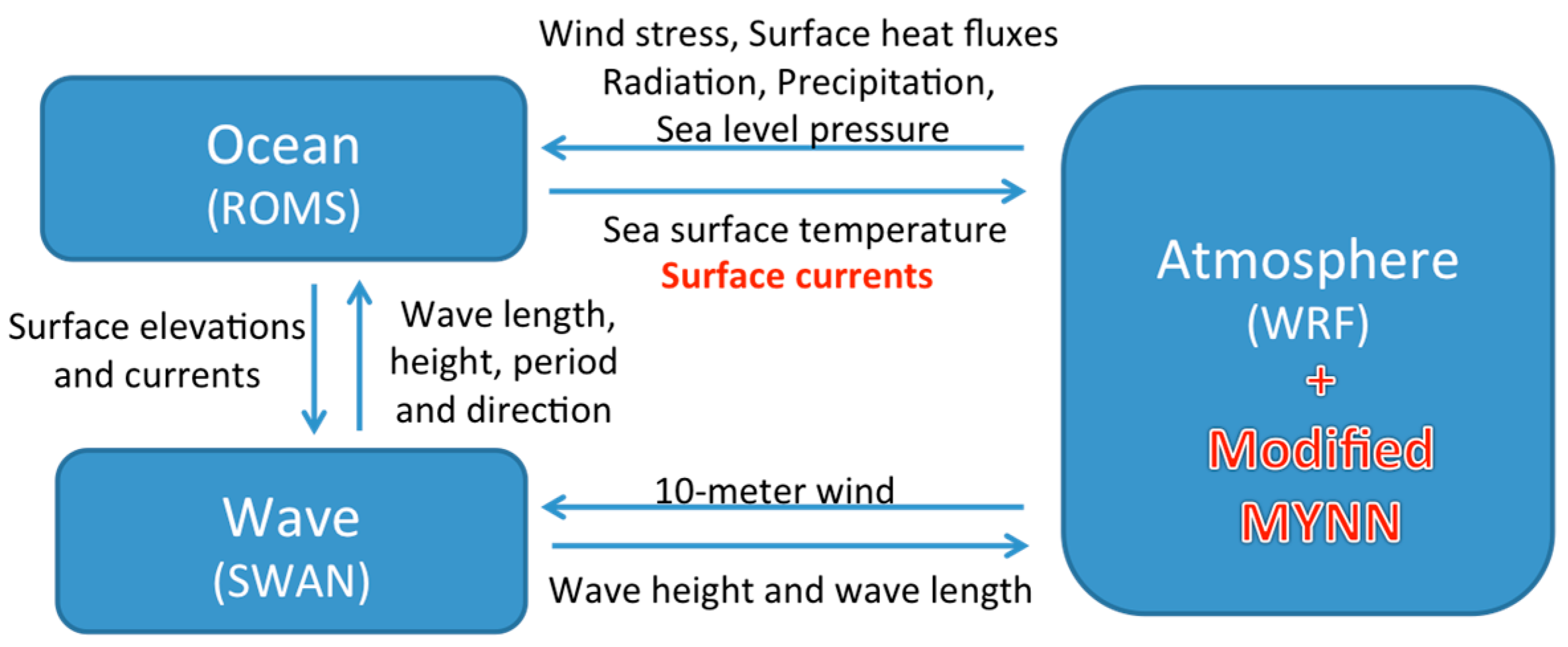
2.1. Coupling between Each Model Component

The momentum and heat fluxes between the ocean and the atmosphere are calculated in the WRF model’s surface layer module, Mellor–Yamada–Nakanishi–Niino (MYNN). The ROMS model is driven by these surface fluxes and, in turn, modifies the WRF model via the SSTs and surface currents that are used in the modified flux calculations (Section 2.2). Therefore, the ROMS and the WRF model are consistent with respect to the momentum and heat fluxes. In the SWAN model, surface wind speed and direction are used in the Komen et al. [43] closure model for the energy transfer from the atmosphere to the wind wave fields. The SWAN model also receives free surface elevations and currents from the ROMS. The ocean surface currents affect the waves by modifying the wind shear (U_wind-U_s, V_wind-V_s) in the calculation of stress and allow current-induced refraction [3,4,34]. In turn, the SWAN model feeds back to the WRF model and ROMS via significant wave height, peak wavelength, peak wave period, and mean wave direction. The atmospheric, ocean, and wave models were synchronized every 10 minutes to exchange data files through the MCT coupler. The details of fields that have been exchanged among these three model components are shown in Figure 1.

2.2. Flux Parameterization and Experimental Design

The momentum flux through the air–sea interface is expressed in terms of wind stress, which is the vertical transfer of horizontal momentum per unit area [44]. The vector wind stress ($\stackrel{\rightharpoonup }{\tau }$) is given by

$$\stackrel{\rightharpoonup }{\tau }=\rho \stackrel{\rightharpoonup }{u_{*}}\left|\stackrel{\rightharpoonup }{u_{*}}\right|,$$

(1)

where $\rho$ is the density of the air, and $\stackrel{\rightharpoonup }{u_{*}}$ is the friction velocity. The friction velocity depends on the vertical wind shear and atmospheric stability. This dependence is expressed by the log wind profile [11]:

$$\overrightarrow{U}\left(z\right)-{\overrightarrow{U}}_s=\overrightarrow{\frac{u_{*}}{k}}\left[\ln \left(\frac{z}{z_0}\right)-\phi \left(z,z_0,L\right)\right],$$

(2)

where $\overrightarrow{U}\left(z\right)$ is the wind velocity at height z (10 m in this case); ${\overrightarrow{U}}_s$ is the velocity of surface ocean current; $u_{*}$ is the friction velocity; $k$ is von Karman’s constant; $z_0$ is the roughness length; $\phi$ is a function of atmospheric stability; and $L$ is the Monin-Obukhov scale length. Given $L$ and a relationship between roughness length and friction velocity, the friction velocity can be obtained from Equation (2).

The sensible and latent heat fluxes over ocean surface are expressed as [11]

$$Q_{sen}=-\rho C_p{\theta }_{*}\left|\overrightarrow{u_{*}}\right|,$$

(3)

$$Q_{lhf}=-\rho L_v{q}_{*}\left|\overrightarrow{u_{*}}\right|,$$

(4)

where $C_p$ is the specific heat of air, $L_v$ is the latent heat of vaporization, and ${\theta }_{*}$ and $q_{*}$ are the scaling parameters analogous to the friction velocity. The roughness lengths for thermal and moisture are taken from the COARE 3.0 bulk algorithm [45]:

$$z_{0\theta }=z_{0q}=min\left(1.1\times {10}^{-4},5.5\times {10}^{-5}R{e}^{-0.6}\right),$$

(5)

where $z_{0\theta }$ is the roughness length for potential temperature, $z_{0q}$ is the roughness length for specific humidity, and R_e is the roughness Reynolds number ($R_e=z_o{u}_{*}/\upsilon$). In this study, four experiments were designed to separate the ocean currents effect on the wind stress from the wave effect. These four experiments differ only in whether ocean currents or sea-state parameters are used in the bulk parameterization to modify the surface roughness. For the control experiment (CTL), wind stress and heat fluxes calculated in the WRF model are based on the Coupled Ocean-Atmosphere Response Experiment (COARE; [45]) 3.0 bulk flux algorithm. Similar to the conventional ocean and atmospheric models, the surface ocean current is neglected in the log wind profile (Equation (2)). The velocity roughness length is specified as

$$z_o=\frac{\alpha u_{*}^2}{g}+\frac{0.11v}{u_{*}}$$

(6)

$$\alpha =0.011+0.007\times min\left(max\left(\frac{U_{10}-10}{8},0\right),1.0\right),$$

(7)

where $z_o$ is roughness length, $u_{*}$ the friction velocity, $g$ the acceleration due to gravity, $v$ the kinematic viscosity, and U₁₀ the 10-m wind. The Charnock parameter α is a nondimensional scaling factor that characterizes the variation of the drag coefficient due to sea state (typically ranging from 0.011 to 0.018). Higher values of α have been used when wave orbital motion reduces the wind shear [11]. However, we have not adapted that type of coupling in this model, and hence use the COARE 3.0 values. The first term is the roughness length associated with gravity waves. The second term is the roughness length for the smooth surface condition, where viscous friction plays a dominant role in the momentum transport [46]. Arguably, additional roughness from capillary waves [44] or additional wind shear through gustiness [47] act to increase the stress for wind speeds from rough 2 to 5 m s⁻¹. This stress is missing in this model, resulting in weaker fluxes and coupling at these wind speeds.

The ocean current experiment (CUR) uses the same COARE 3.0 bulk flux algorithm as the CTL experiment, except that the ocean surface currents are allowed to modify the vertical wind shear, as given by Equation (2). In this two-way coupled configuration, the current-modified wind stress is sent back by the MCT coupler to drive the ocean currents.

In the wave and wind stress coupled experiment (WAV), the surface roughness length is scaled by the wave slope [48]:

$$z_o=1200\times H_s\times {\left(\frac{H_s}{L_p}\right)}^{4.5}+\frac{0.11v}{u_{*}},$$

(8)

where $H_s$ is significant wave height and $L_p$ is the wavelength at peak of the wave spectrum. Therefore, $H_s/L_p$ is approximately the slope of the dominant waves. Studies have shown that Taylor and Yelland’s wave-slope scaling surface roughness algorithm performs better than a standard bulk flux formulation in a wide range of conditions [2,27]. This model includes sea-state dependency beyond what was captured in COARE 3.0 but is reasonably similar to COARE 3.0 for typical ocean conditions. There are many other sea state dependent parameterizations [11,27,49,50] that could have been used to examine dependency on sea state. For this study, we selected only one model with the goal of showing that sea state could be important in coupled modeling.

In the wave–currents–wind–stress three-way coupling experiment (CUR_WAV), we substituted surface wind for the wind shear between the surface wind and the ocean currents, and used the Taylor and Yelland [48] algorithm for surface roughness length calculation.

Table 1. Description of the experiments performed in this study. The ${\stackrel{\rightharpoonup }{U}}_{10}$ is the 10-m wind, and ${\stackrel{\rightharpoonup }{U}}_{CUR}$ is the ocean surface current. CTL, control experiment; CUR, ocean current experiment; WAV, wave experiment; CUR_WAV, wave–currents–wind–stress three-way coupling experiment; COARE, Coupled Ocean-Atmosphere Response Experiment.

Experiments	Roughness Length Algorithm	Wind Input for Surface Stress Formulation
CTL	COARE 3.0	${\stackrel{\rightharpoonup }{U}}_{10}$
CUR	COARE 3.0	${\stackrel{\rightharpoonup }{U}}_{10}-{\stackrel{\rightharpoonup }{U}}_{CUR}$
WAV	Taylor and Yelland	${\stackrel{\rightharpoonup }{U}}_{10}$
CUR_WAV	Taylor and Yelland	${\stackrel{\rightharpoonup }{U}}_{10}-{\stackrel{\rightharpoonup }{U}}_{CUR}$

lists the key aspects of all the simulations made in this study.

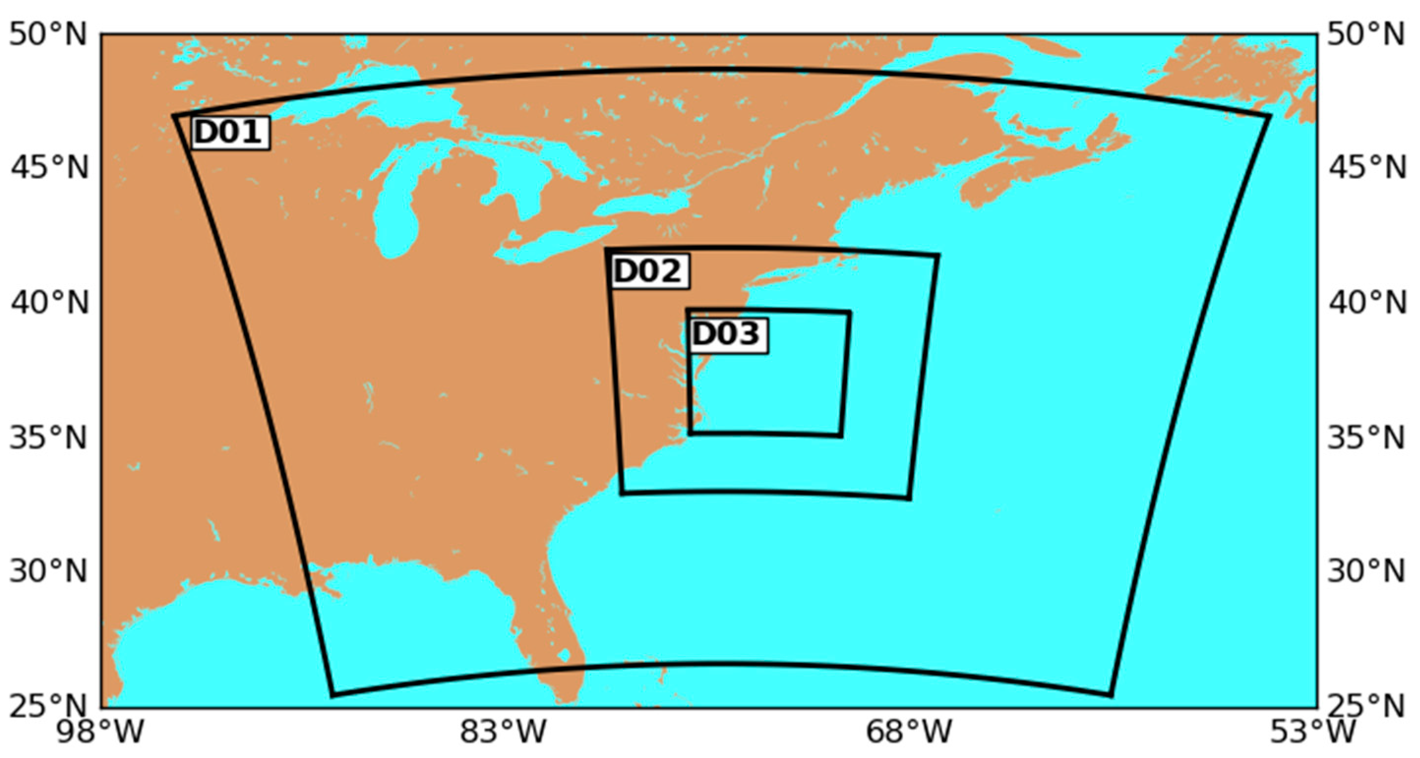
2.3. Experiment Details

For the COAWST atmospheric component, we used WRF version 3.6.1 to make simulations over the U.S. East Coast (Figure 2). The WRF simulations consist of three domains (two-way nesting) with grid spacing of 30 km, 10km, and 3.3 km, respectively. This configuration allows us to simulate key precursor synoptic phenomena (e.g., jet streaks, troughs) on the parent domain, and smaller-scale phenomena on the inner domains. The WRF simulations begin at 00 UTC 1 October 2012, with initial and boundary conditions from the 6 hourly National Centers for Environmental Prediction (NCEP) Operational Global Final Analyses dataset, on a 0.5° × 0.5° grid. The 30 km and 10 km domains use the Kain-Fritsch cumulus scheme [51], whereas the 3.3 km domain does not require cumulus parameterization because convection at that scale is explicitly resolved. The MYNN planetary boundary layer scheme, in conjunction with the MYNN surface layer scheme based on Monin–Obuhklov similarity theory, is used in the three domains. Shortwave and longwave radiation are parameterized using the Rapid Radiative Transfer Model (RRTMG; [52]).

For the COAWST ocean component, we used ROMS release 748 [53]. The ROMS simulations also consist of three domains with grid spacing of 30 km, 10 km, and 3.3 km, respectively. ROMS domains are within the bounds of the corresponding WRF domains for stability. Because the WRF and ROMS grid are not co-located, the Spherical Coordinate Remapping Interpolation Package (SCRIP) is used to compute interpolation weights between WRF and ROMS. ROMS is initialized with HYCOM+NCODA global 1/12° analysis (hot start) to reduce the spin-up time. No spikes due to instability are seen in modeled fields during the one month simulation, which is expected since the ocean model is initialized according to realistic conditions. Therefore, no spin up time was used in this study.

For the COAWST wave component, we used SWAN version 40.91A [54]. The physical processes accounted for in SWAN include wave generation by wind, wave propagation in time and space, three- and four-wave interactions, and whitecapping. SWAN simulations are performed on the same grid as ROMS. The SWAN model is initialized with a completely flat sea state. The spin-up period required to generate the wind waves is typically 12 to 18 hours [55]. The boundary conditions for SWAN were obtained from the WAVEWATCH III model output.

3. Modeling Results

The effects of currents and waves on air–sea momentum and heat flux exchanges are investigated by coupling wind stress with waves/currents in a two-way fashion. The upper ocean and MABL response to the coupling of wind stress with currents/waves are also examined in this study. In general, our results highlight the substantial impact of coupling currents/waves with wind stress on the air–sea flux exchange and ocean upwelling over the Gulf Stream. We find that the current effect has a dominant impact on MABL and the wave response in the CUR_WAV experiment. Alternating positive and negative bands of Ekman pumping vertical velocity changes along the Gulf Stream are visible in the current–wave–stress coupling experiment. This small-scale feature is also revealed by four year averages of 25 km scatterometer observations [18].

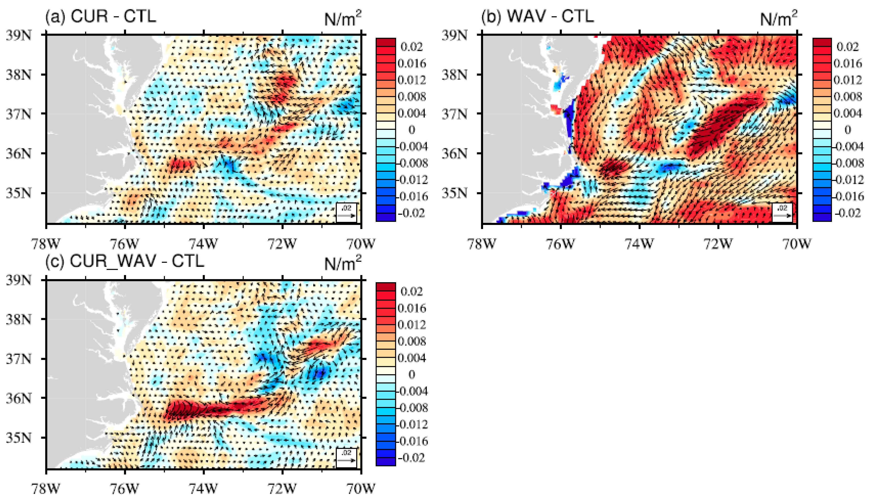
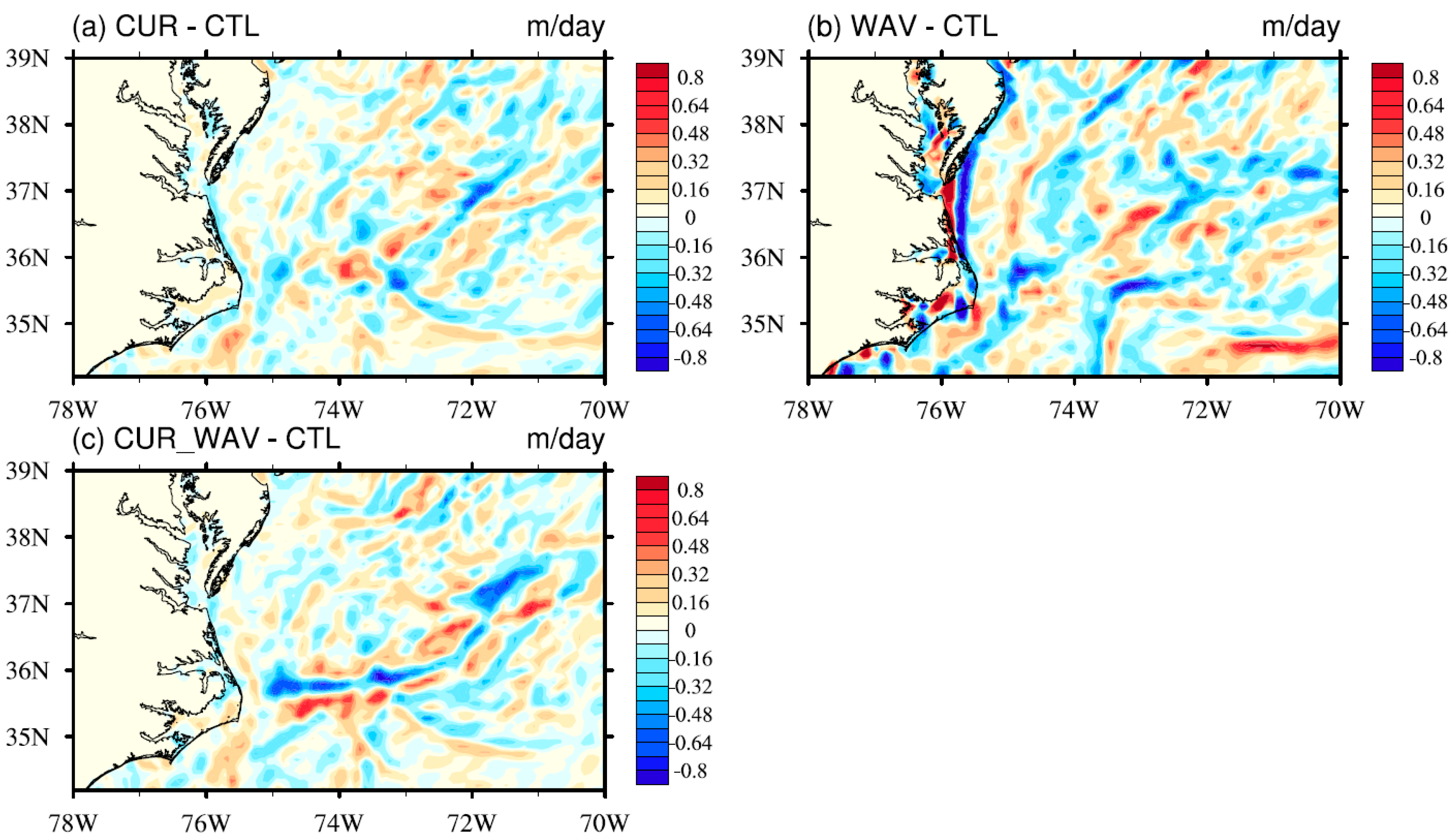
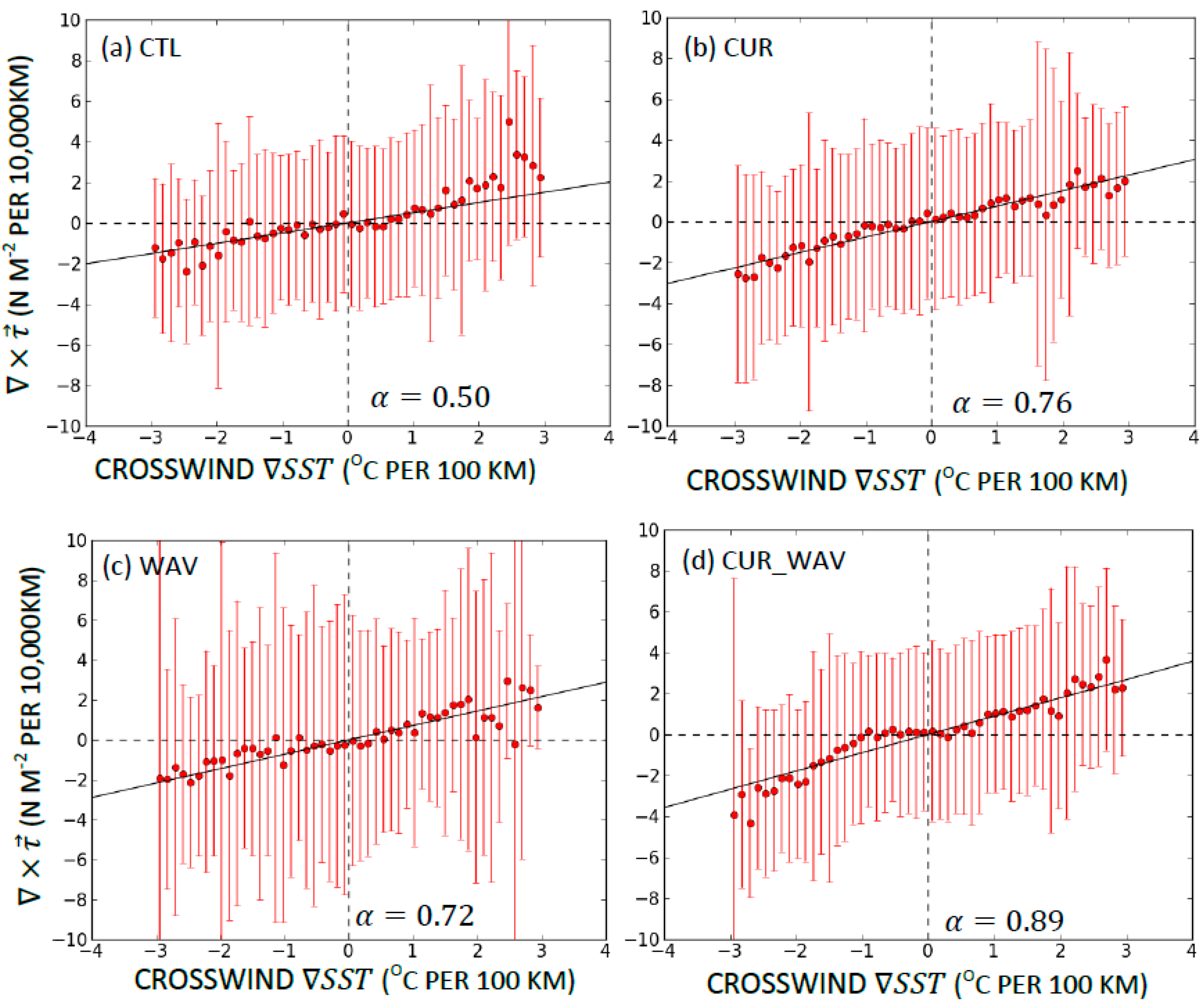
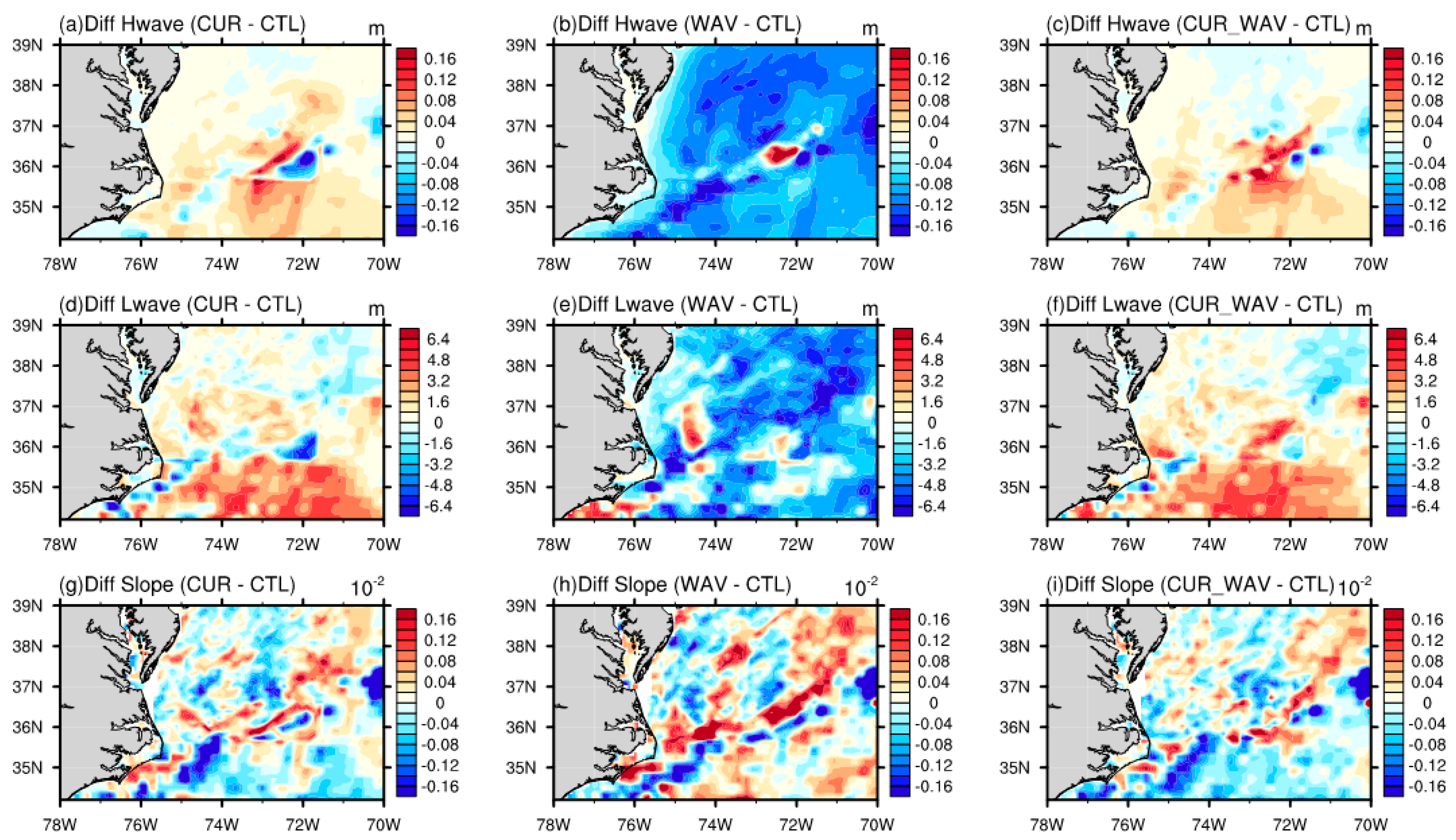
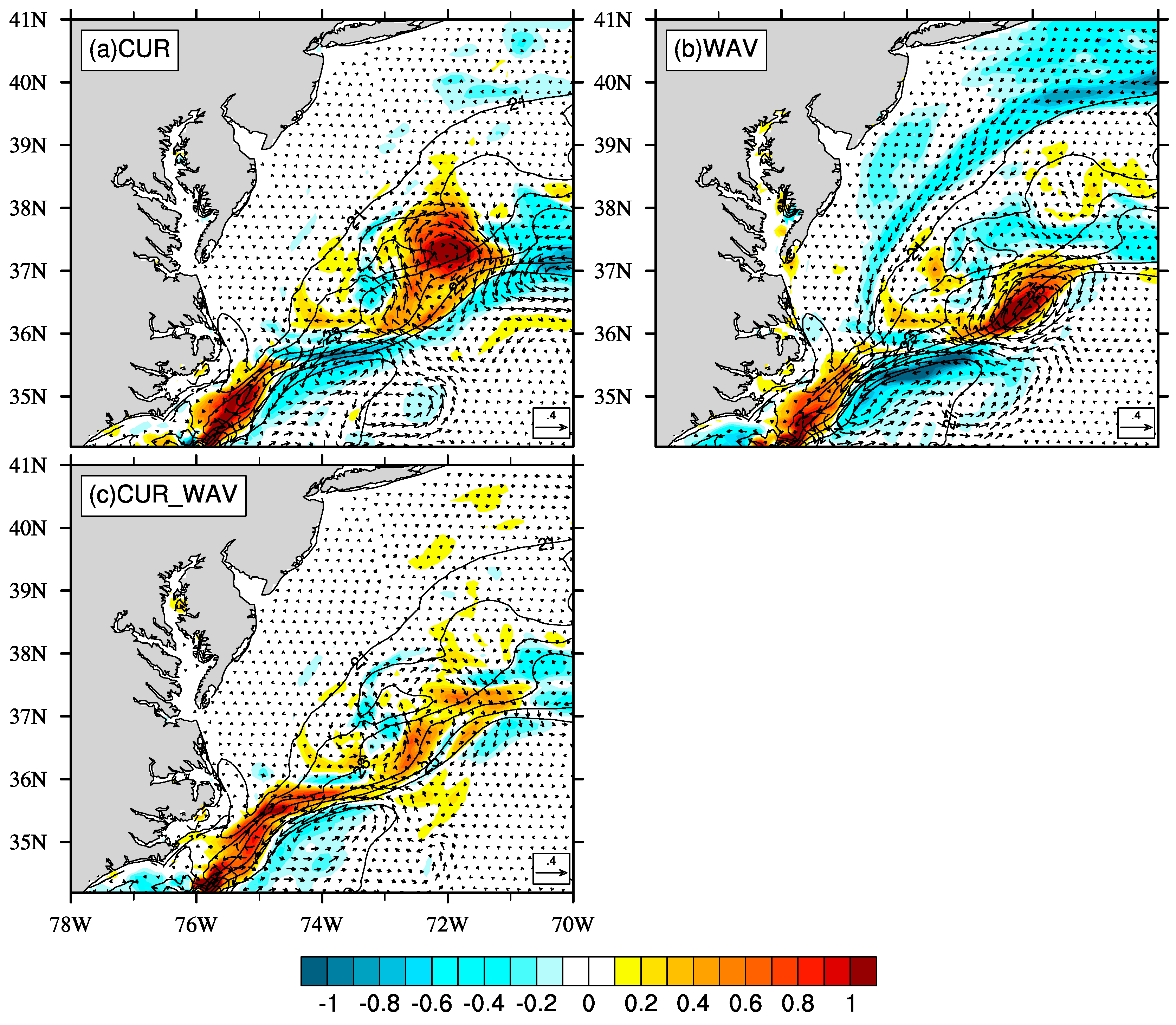
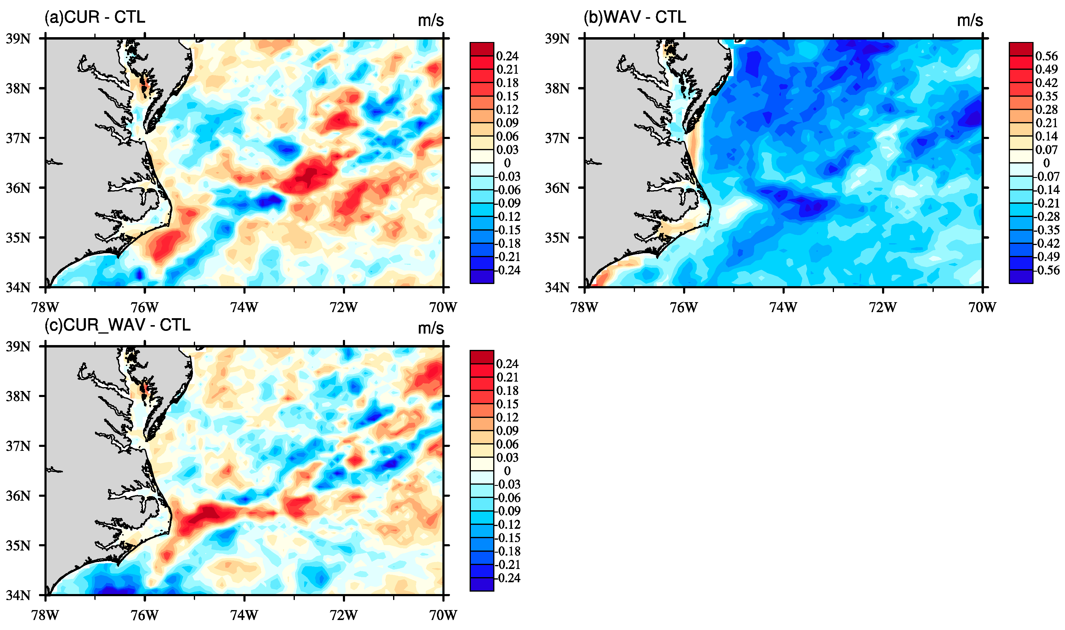
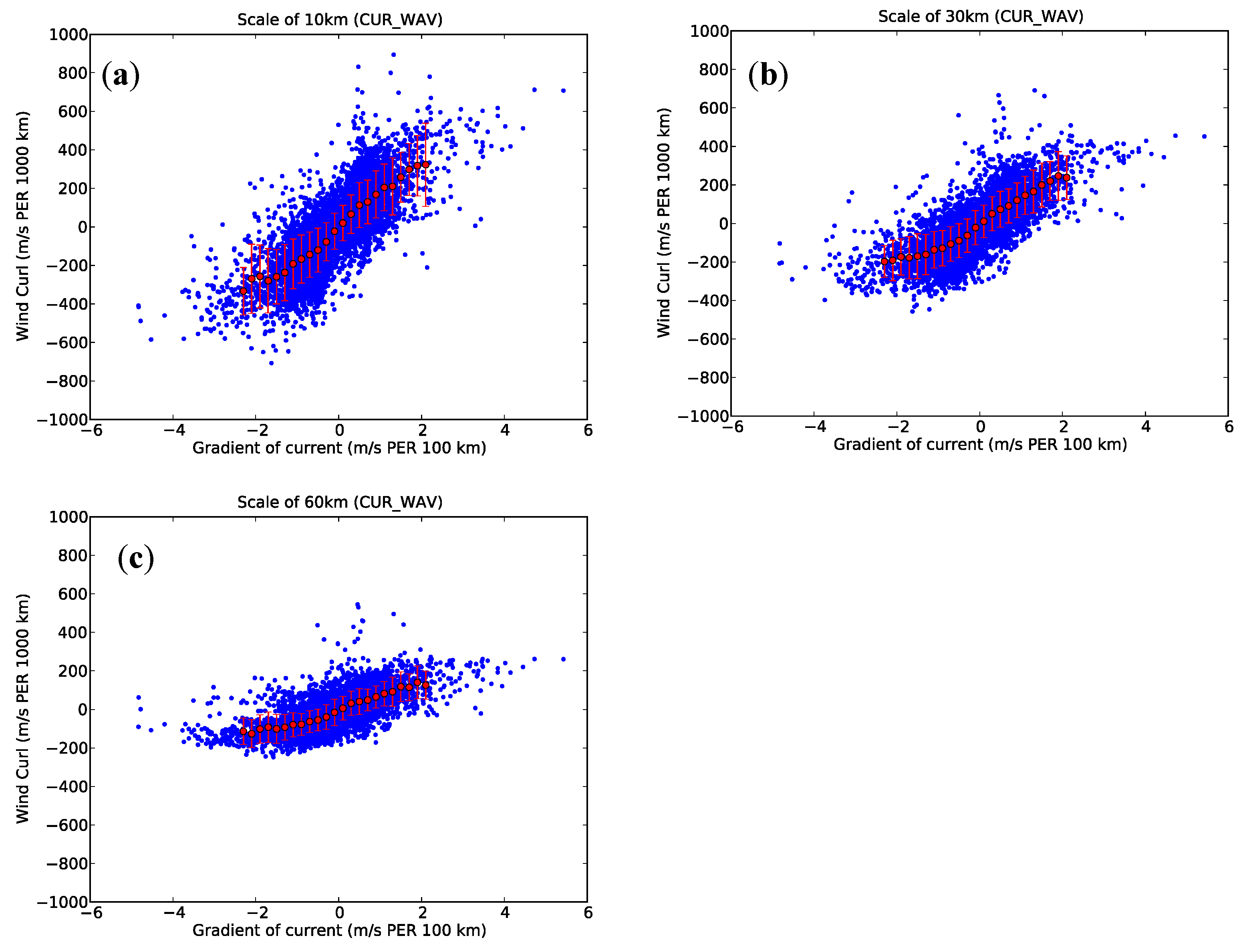
3.1. Impact on the Wind Stress, Its Curl, and Waves

To investigate the impact of coupling ocean currents/waves and wind stress on oceanic and atmospheric circulations, we compared each of the three coupled simulations with the CTL simulation. Figure 3a–c shows changes of wind stress due to surface currents and wind stress coupling (CUR-CTL), wave and wind stress coupling (WAV-CTL), and current–wave–stress three-way coupling (CUR_WAV-CTL), averaged over a 30 day period (1–30 October 2012). Substantial wind stress increases (>15%, Figure 3c) by coupling currents, waves, and wind stress simultaneously are observed at the Gulf Stream, with only small changes elsewhere. A similar response spatial pattern is seen in the current–stress coupling (Figure 3a), while the magnitude of wind stress change in current–stress coupling is smaller than in the wave–current–stress coupling. As we can see from Figure 3b, there is a considerable wind stress increase outside the Gulf Stream due to the wind stress and wave coupling. However, there is only a moderate increase/decrease outside the Gulf Stream in the wave–current–stress coupling. This indicates that the current effect, on average, roughly cancels out the wave effect outside the Gulf Stream. The vector difference of wind stress (Figure 3c) shows that an additional local curl of wind stress is generated at the Gulf Stream in the CUR_WAV experiment. Alternating positive and negative bands of changes for the Ekman pumping vertical velocity in response to the changes of wind stress curl (Figure 4c) are seen along the Gulf Stream, with magnitudes exceeding 0.3 m/day (95th percentile). This small-scale feature is also revealed by four year averages of 25 km scatterometer observations [18]. Unlike the wave–stress coupling, no substantial change of Ekman pumping vertical velocity is seen near the coastline. In general, the changes of wind stress and its curl in the wave–current–stress coupling is not a linear combination of changes in the wave–stress coupling and current–stress coupling experiments.

Previous observational and model studies [56,57,58] found that the curl of surface wind stress is linearly correlated with the crosswind component of the SST gradient over SST fronts, and the sensitivity of the wind stress curl to the crosswind SST gradient is defined as below:

$$\alpha =\frac{\nabla \times \overrightarrow{\tau }}{\nabla SST\times \frac{\overrightarrow{\tau }}{\left|\overrightarrow{\tau }\right|}},$$

(9)

where α is the coupling coefficient, $\overrightarrow{\tau }$ is the surface wind stress, and ∇SST is the gradient of the sea’s surface temperature. The relationships of wind stress curl and the SST gradient in the four model configurations are quantified in Figure 5 using binned scatterplots. The statistics are computed over the region 35.8N–39.2N, 76W–72W using 30 day averaged fields. All experiments do well in producing a positive relationship between wind stress curl and the crosswind SST gradient. The coupling coefficients for CTL, CUR, WAV, and CUR_WAV are 0.5, 0.76, 0.72, and 0.89 × 10⁻² N m⁻² °C⁻¹, respectively. The uncertainty for the slope is 0.068, 0.0072, 0.0049, and 0.005 × 10⁻² N m^-2 °C⁻¹, respectively. The 10 year averaged coupling coefficient derived from buoys and satellite observed SST and surface wind is 0.91× 10⁻² N m⁻² °C⁻¹ near the Gulf Stream [59], which is very close to the coupling coefficient from the CUR_WAV experiment. The coupling coefficient, which numerical models often underestimate [60,61], increases by 78% after adding the wave–current–stress coupling (CUR_WAV) to the control case’s physics. Moreover, coupling currents and/or wave with wind stress also decreased the uncertainty of the coupling coefficient by one order of magnitude.

The wave/current-induced wind stress feeds back to waves through the two-way coupled model configuration, assuming the MABL winds do respond to the stress parameterizaiton, as seems likely to be the case. To investigate the wave response to the wave-current-stress coupling, we compare the significant wave height, wavelength, and wave slope between the coupled and CTL experiments. The wave response to the wave–current–stress coupling (CUR_WAV) is different from the wave response to the wave-stress (WAV) coupling. Coupling waves and wind stress alone (WAV) significantly increase the wind stress (Figure 3b). However, waves get less energy with decreased significant wave height (Figure 6b) over a large area of the model domain. In contrast to the WAV experiment, the significant wave height (Figure 6c) and wavelength (Figure 6f) generally increase in the CUR_WAV experiment, which indicates that waves get more energy to grow by coupling waves, currents, and stress simultaneously. The huge difference of sea-state change patterns between the WAV and CUR_WAV experiments strongly suggests that current-stress coupling plays a dominant role in the sea state change in the CUR_WAV experiment. We compare patterns of sea state changes in the CUR_WAV (Figure 6c,f,i) with patterns of sea-state changes in CUR (Figure 6a,d,g). As expected, the sea-state change patterns in the CUR_WAV and CUR experiments are very similar. There are two mechanisms that allow ocean currents to modify the sea-state in CUR_WAV. First, currents modify the surface wind by changing the wind shear ($\overrightarrow{U}\left(z\right)-{\overrightarrow{U}}_s$). Second, currents reflect and trap gravity waves near the Gulf Stream [62,63]. The second mechanism exits in both the WAV and CUR_WAV experiments. Therefore, a current-induced surface wind change might play a dominant role in the sea-state response patterns in CUR_WAV. To explore the contribution of ocean currents on surface wind change, we use the equation for a log wind profile:

$$\overrightarrow{U}\left(z\right)={\overrightarrow{U}}_s+\overrightarrow{\frac{u_{*}}{k}}\ln \left(\frac{z}{z_0}\right)-\overrightarrow{\frac{u_{*}}{k}}\phi \left(z,z_0,L\right),$$

(10)

where the definitions of each symbol in Equation (10) is same as those in Equation (2). For convenience, we name the terms on the right side as current term, log term, and stability term, respectively. Histograms of difference for each term between the CUR_WAV and WAV experiments for the log equation are computed over the regions with strong currents (Figure 7a, |Us| > 1 m/s) and weak currents (Figure 7b, |Us| < 1 m/s) using a 6 hourly model output. Recall that the three changes add up to the change in the wind mean wind speed at a height of 10 m. The currents have a much larger impact on the wind speed change than the roughness change (log term) over the strong current region. In the absence of other feedback changing the wind, negative changes in the current term are from conditions where the currents reduce the wind shear, and positive changes are from cases where the wind and currents are opposed. The thermodynamic changes in the atmosphere cause additional strong feedback, which changes this relatively straightforward perspective. Interestingly the changes in currents are roughly cancelled by the changes in stability term. While there are large changes in winds very near the surface (not shown), and in the stress, the winds at a 10 m elevation change little due to additional coupling mechanisms. Thus, the currents have a much larger impact on the coupled system than is suggested by changes in U(10). The wave model is parameterized in terms of U(10), and the surface current, rather than stress and current, and therefore is likely to underestimate the sensitivity of sea state to stress. Consider further that wave-current interactions cause changes in the sea state by changing the wavelength of the gravity waves. This impact appears as a change in roughness length, and hence contributes directly to the change in the log-profile term and less directly to the stability term. There are many coupling and feedback systems in a two-way coupled ocean/wave/atmosphere model.

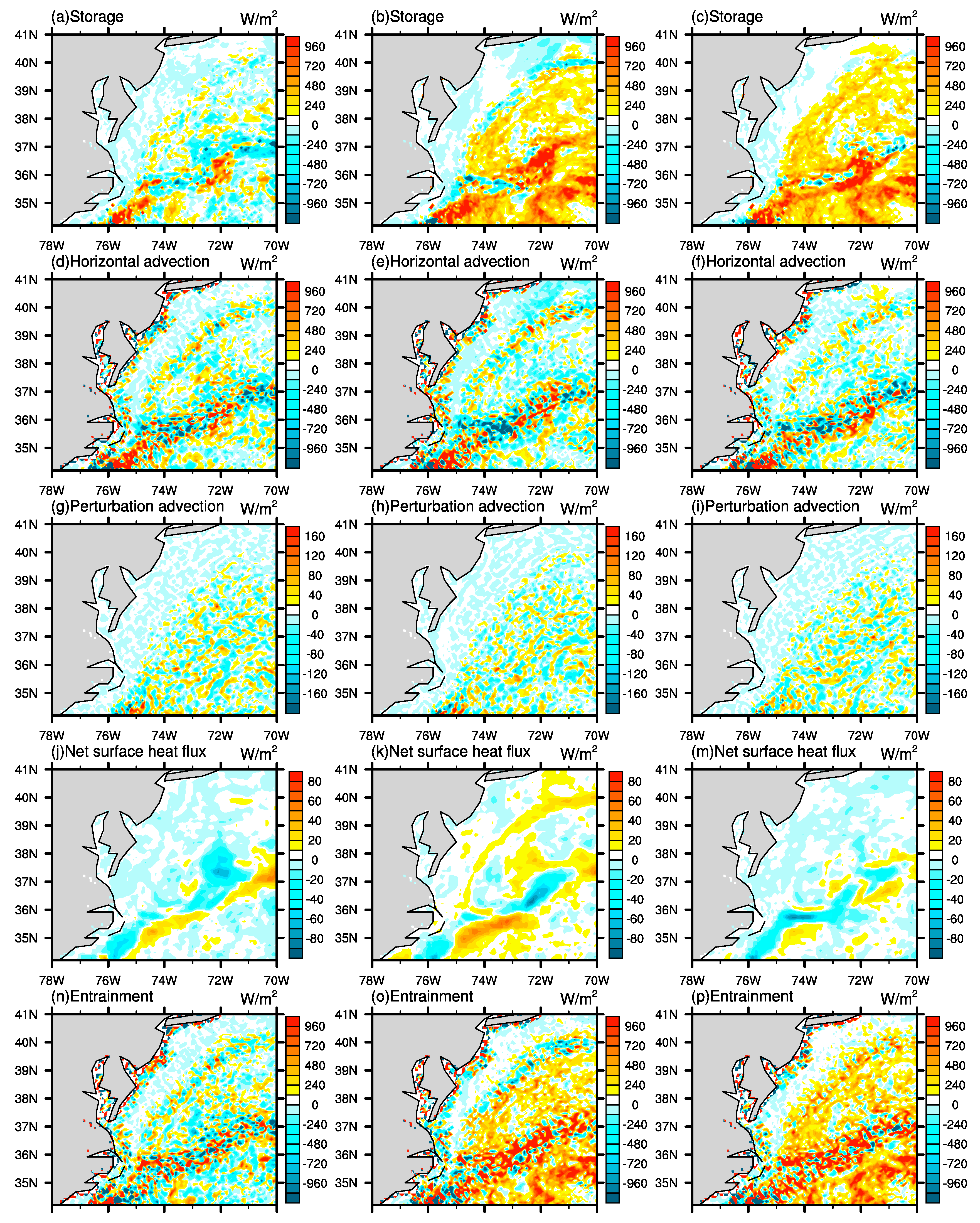
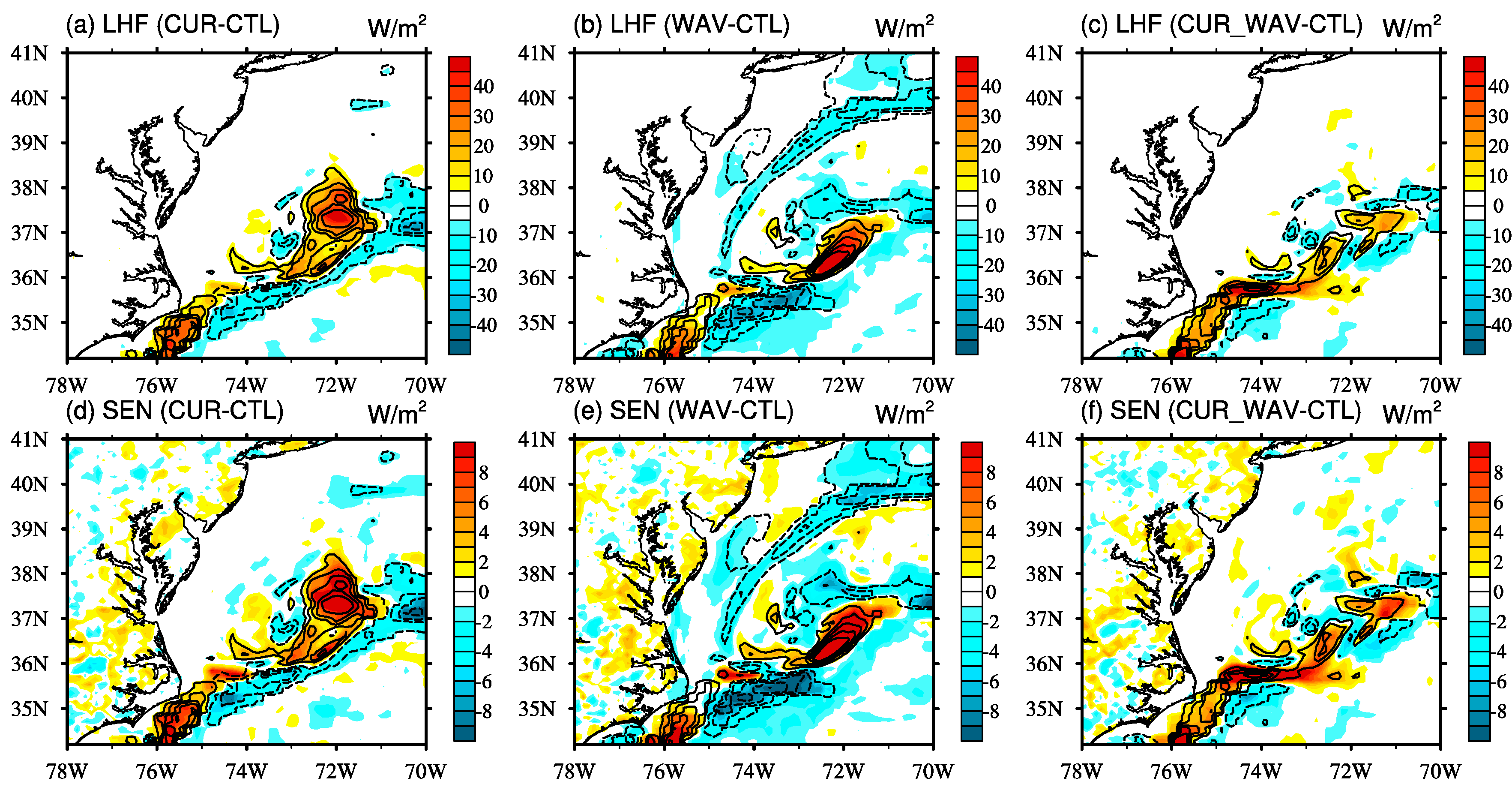
3.2. Impact on SST and Heat Fluxes

In this sub-section, we investigate the impact of coupling ocean currents/waves and wind stress on SST and surface heat flux. Figure 8a shows the 30 day averaged difference of SST and ocean surface currents between the CUR and CTL experiments. The magnitude of the SST’s change is up to 1.3 °C, and changes exceeding 0.6 °C (95th percentile) are located within the ocean frontal region. The magnitude of ocean currents change is up to 0.3 m/s. The anti-cyclonic and cyclonic surface currents anomalies occur at the same location as the cold and warm SST anomalies, which is also revealed from satellite observations [16]. This substantial SST and ocean current change can further impact the stability, turbulent fluxes, and wind fields within the MABL through air–sea interaction. Similar to the effects of currents and wind stress coupling, substantial SST and ocean current changes (Figure 8b) due to wave and wind stress coupling are found near the SST front region in the shape of warm/code core eddies. In addition, there is a band of cold SST anomalies collocate with considerable current anomalies (>0.1 m/s) near the north wall of the ocean frontal area. In the wave–current–stress coupled experiment, SSTs increase exceeding 0.4 °C (95th percentile, Figure 8c) are associated with local current anomalies exceeding 0.1 m/s (95th percentile, Figure 8c), which are seen at the Gulf Stream. Comparing to the CUR and WAV experiments, the magnitudes of SST change and surface current change (black vectors, Figure 8c) are smaller in the three-way coupled experiment (CUR_WAV).

Because of the substantial change in SSTs due to coupling wind stress with ocean current and waves, we perform a mixed layer heat budget analysis to investigate the physical processes happening in the ocean mixed layer and their contribution to the SST change. Derived from the conservation of mass and heat equations, the heat budget equation is expressed as [64]

$$\begin{gathered} h{\partial }_{t}T=-h\overrightarrow{U}·\nabla T-\nabla ·{{\displaystyle \int }}_{-h}^0\tilde{\overrightarrow{U}}\tilde{T}dz \\ -\left[T-T\left(-h\right)\right]w_e\left(-h\right)+\frac{F_{sol}}{{\rho }_0{c}_p}\left[I\left(0\right)-I\left(-h\right)\right] \\ +\frac{F_{nsol}}{{\rho }_0{c}_p}-\overline{w^{\prime }{T}^{\prime }}\left(-h\right)+h{A}_h{\nabla }^{2}T, \end{gathered}$$

(11)

where $T$ is the temperature; $\overrightarrow{U}=\left(u,v\right)$ are the horizontal velocity components; h is the mixed layer depth (MLD); $w$ is the vertical velocity component; $F_{sol}$ is the downward shortwave radiation at the sea surface; $I\left(-h\right)$ is the fraction of shortwave radiation, which penetrates to the depth −h; $F_{nsol}$ is the sum of the sensible, latent, and net longwave radiative flux; ${\rho }_0$ is the density of the ocean water; $c_p$ is heat capacity of ocean water; and $A_h$ is the horizontal diffusivity. For any variable a, the depth average over the mixed layer is defined as

$$a=\frac{1}{h}{{\displaystyle \int }}_{-h}^{0}adz,$$

(12)

The entrainment velocity at a mixed layer base, $w_e\left(-h\right)$, is defined as the vertical flow of material across the surface $z=-h$ [65]:

$$w_e\left(-h\right)=w\left(-h\right)+{\partial }_{t}h+U\left(-h\right)·\nabla h-A_h{\nabla }^{2}h,$$

(13)

The MLD h(x, y, t) is determined using ocean temperature profiles. In brief, the MLD is the depth at which the temperature has changed by an absolute temperature difference of 0.8 °C from the temperature at 10 m beneath the ocean surface [66,67].

The left side of Equation (11) is the change of the depth-averaged temperature, which we will refer to as the heat storage. The first two terms on the right side of Equation (11) are the horizontal heat advection by the depth-averaged current and the perturbation of the mean current. The third term is the entrainment rate at the mixed layer bottom. The fourth and fifth terms are the net shortwave radiation absorbed throughout the layer and the net turbulent fluxes and longwave radiation at the ocean surface. The last two terms are the turbulent heat flux at the bottom of the mixed layer and the horizontal diffusion, respectively. ROMS uses third-order upwind scheme for horizontal advection [68] and a fourth-order centered scheme for vertical advection. The horizontal diffusion in Equation (11) is set to zero because there is no explicit horizontal diffusivity in the ROMS model. The two-dimensional maps of differences between CTL and coupled experiments for each term in the heat budget are shown in Figure 9. A strong increase of heat storage (exceeding 960 W/m², Figure 9b,c) is seen at the Gulf Stream in both WAV and CUR_WAV experiments, while both an increase and decrease of heat storage (Figure 9a) are seen at the Gulf Stream in the CUR experiment. The amount of the changes in horizontal advection (Figure 9d–f) and entrainment (Figure 9n–p) are an order of magnitude greater than the changes in the net surface heat flux (Figure 9j–m) in all three coupled experiments. Positive pattern correlation between horizontal advection (Figure 9d) and the heat storage (Figure 9a) change is seen in the CUR experiment, which indicates that the horizontal advection is the major contributor to the SST change due to current-stress coupling. A similar pattern correlation between heat storage (Figure 9b) and horizontal advection (Figure 9e) is seen at the Gulf Stream in the WAV experiment. In the CUR_WAV experiment, the sign of the horizontal advection (Figure 9f) change is opposite to the sign of the heat storage change (Figure 9c) in a large portion of the model domain. A negative correlation is also found between the net surface heat flux (positive sign means a downward heat flux from the atmosphere to the ocean, Figure 9m) and total heat storage change (Figure 9c). Overall, the vertical entrainment plays a more important role in the SST change for the CUR_WAV experiment than for the CUR experiment. This is expected, since the curl of the stress near the Gulf Stream is greatest in the CUR_WAV experiment.

The change in SST and ocean currents via wind stress and current/wave coupling leads to changes in surface heat fluxes. Figure 10 shows the 30 day averaged difference of latent heat flux (LHF) and the sensible heat flux (SEN) between coupled and CTL experiments. For reference, the mean SST difference is overlaid in Figure 10 as contours. For CUR and CUR_WAV experiments, substantial changes of the mean LHF (up to 40 W/m², Figure 10a,c) and SEN (up to 8 W/m², Figure 1d,f) are seen at the Gulf Stream, with only small changes occurring elsewhere. For the WAV experiment, substantial LHF (Figure 10b) and SEN (Figure 10e) changes are seen not only at the Gulf Stream region, but also to the north of the Gulf Stream. A pattern correlation between the SST change and heat flux change is seen in all three coupled experiments, which suggests that the SST change plays an important role in the heat flux change. According to the bulk flux formula, the LHF is a function of surface wind speed, relative humidity, SST, air temperature, and MABL stability. We calculate the impact of each term of the bulk flux formula on the LHF to determine the contribution of different MABL processes to the LHF change. The impact of surface wind speed on the LHF is expressed as

$$I=\frac{\Delta LHF}{\Delta U_{10}}·\sigma U_{10},$$

(14)

where $I$ is the impact, $\Delta LHF$ is the difference of LHF between the coupled and CTL experiments, $\Delta U_{10}$ is the differential 10 m wind, and $\sigma U_{10}$ is the standard deviation of the 10 m wind from the CTL experiment. We estimate the sensitivity of LHF to the surface wind shear, air–sea temperature difference, and humidity difference by comparing the impact histograms in Figure 11. In the CUR_WAV experiment (Figure 11c), the modes for the impact of 10 m wind shear, air–sea temperature difference, and humidity difference are 0.75 W/m², 3.75 W/m², and 5.25 W/m², respectively. The LHF change is most sensitive to the air–sea humidity difference, which is similar to the CUR and WAV experiment (Figure 11a,b). Interestingly, histograms for the CUR_WAV experiment (Figure 11c) are very similar to the averaged histograms (Figure 11d) of the CUR and WAV experiments.

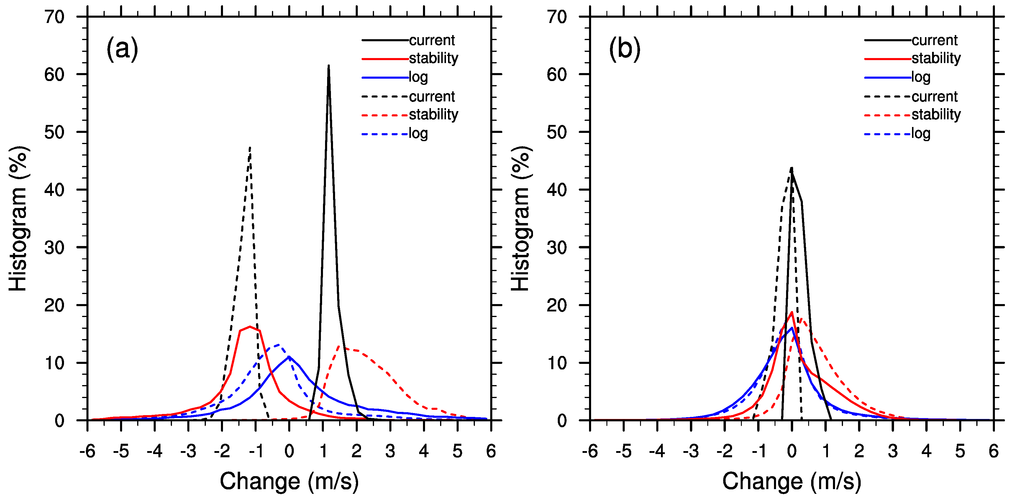
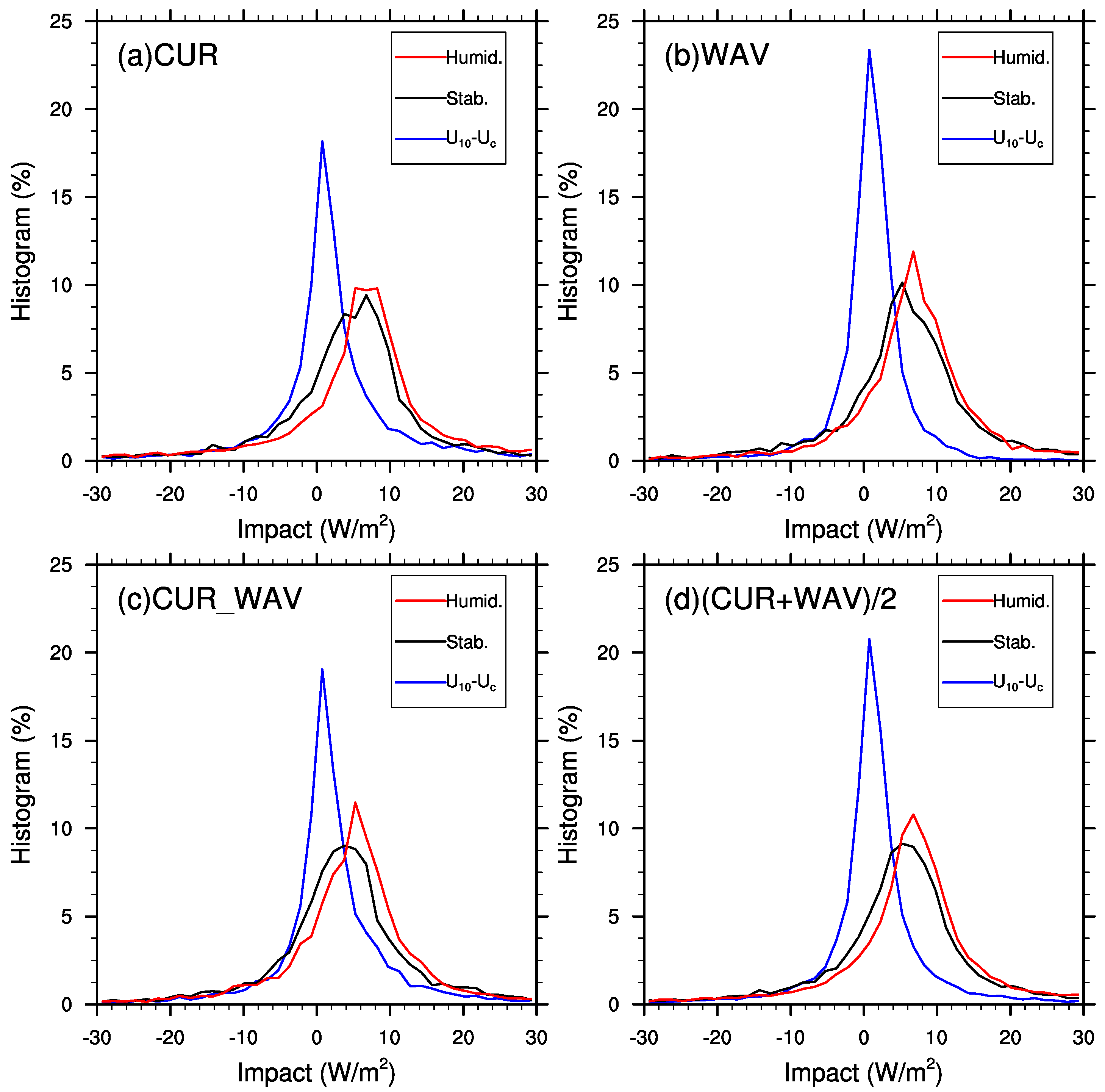
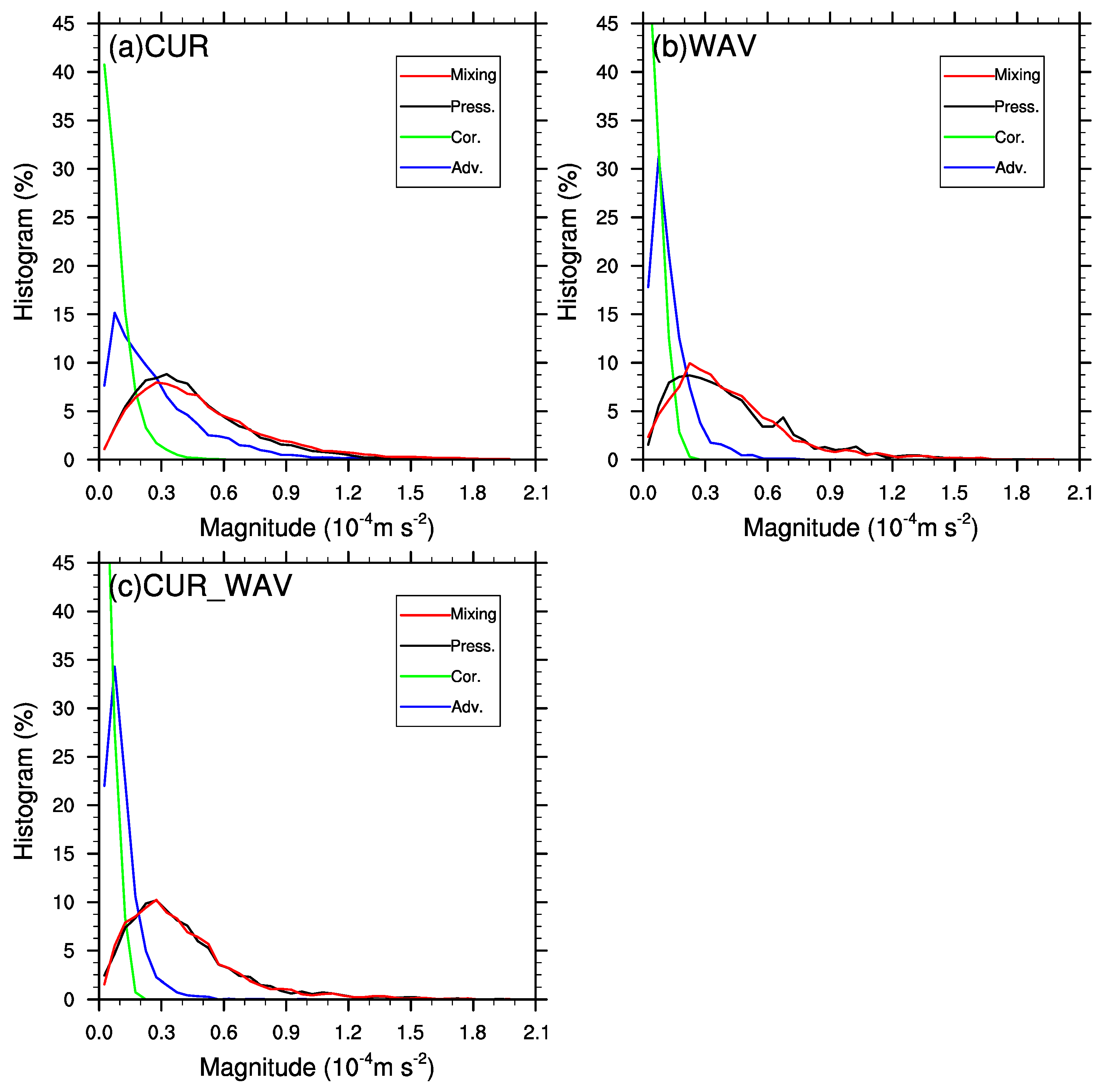
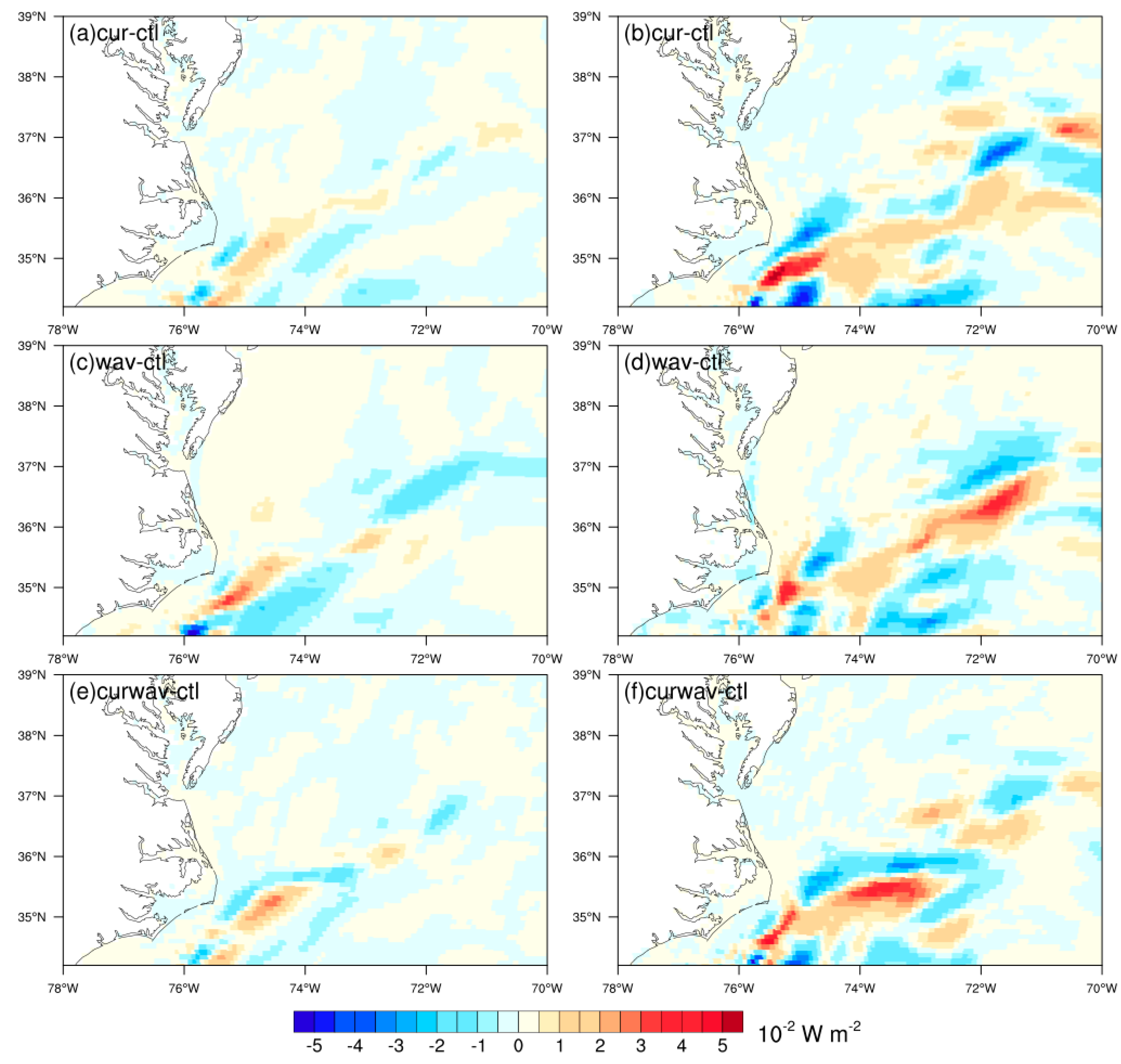
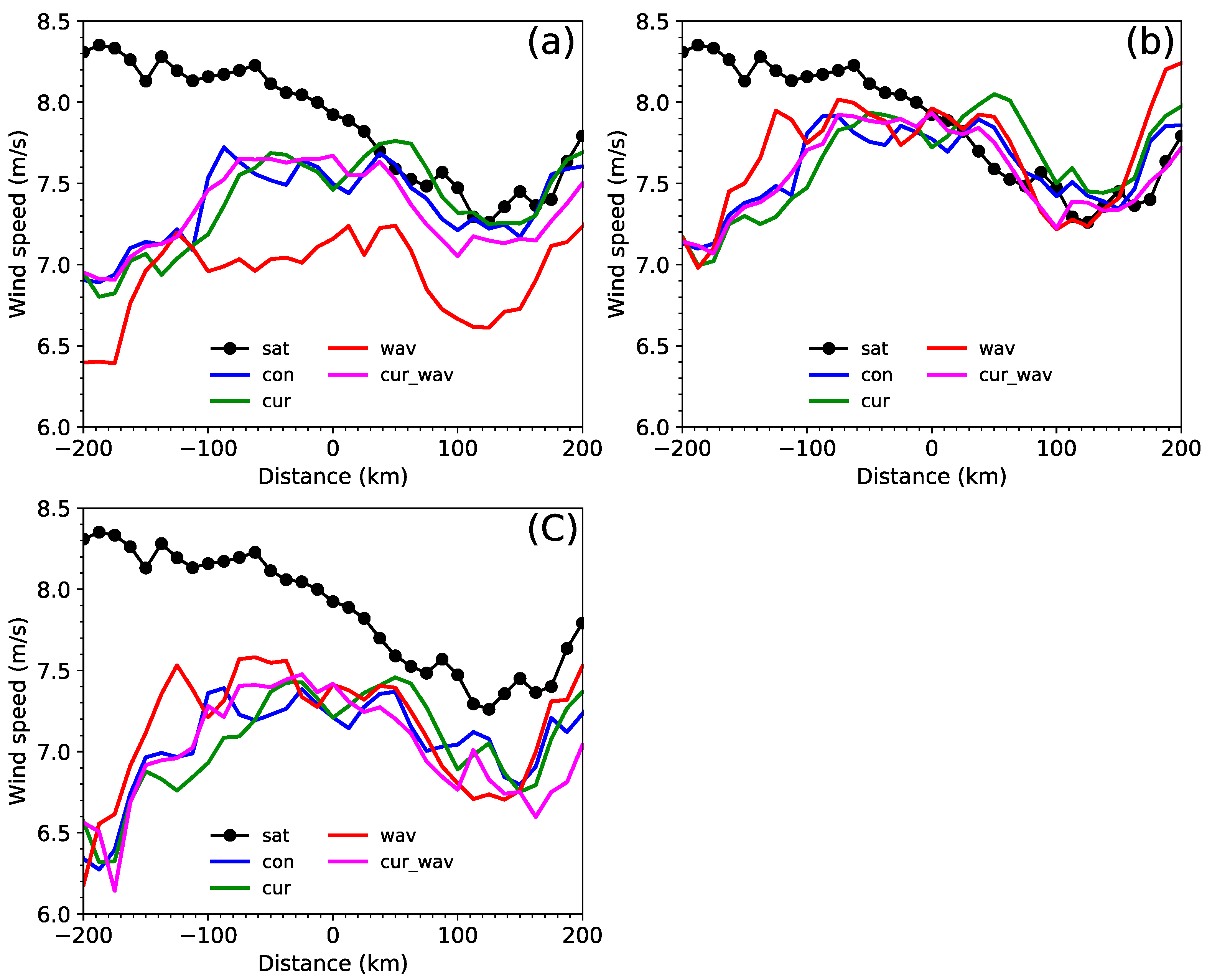
3.3. Impact on Surface Wind and Wind work

Since coupling wind stress with ocean currents and waves substantially alters the mean momentum and heat exchange at the air–sea interface, the surface wind response to those changes is investigated in this section. Moderate 10-m wind (defined by the World Meteorological Organization as ‘surface wind’) changes exceeding 0.15 m/s are seen at the Gulf Stream in both the CUR_WAV (Figure 12c) and CUR (Figure 12a) experiments. Recall that in high current regions, changes in the current are countered by changes in the shape of the wind profile, resulting in only small changes at a 10 m height, rather than closer to the surface. Nevertheless, we focus on the changes in wind at 10 m because these changes can be compared to dependencies seen in satellite observations (e.g., Figure 5), which is the wind input into the wave model. In the WAV experiment (Figure 12b), the magnitude of surface wind speed change is twice as large as the changes in the CUR_WAV and CUR experiments, and only negative values are seen in most of the model domain. Pattern correlation between surface wind change (Figure 12a,c) and SST change (Figure 8a,c) is seen in both CUR and CUR_WAV coupling. This positive correlation between SST and surface wind has been observed in regions of strong SST fronts all over the World Ocean [56]. There is ongoing debate on the relative contributions of stability and pressure gradient forces to the surface wind modification at the SST front region [57,69,70,71]. To investigate the contribution of MABL physical processes to the surface wind change, we apply momentum budget analysis to the surface wind in four experiments. The momentum budget can be written in the model coordinate (x, y, η) [71]:

$$\begin{gathered} \frac{\partial \stackrel{\rightharpoonup }{u}}{\partial t}=-\overrightarrow{u}·\nabla \overrightarrow{u}-\frac{d\eta }{dt}·\frac{\partial \overrightarrow{u}}{\partial \eta }-f\overrightarrow{k}\times \stackrel{\rightharpoonup }{u}-\left\{\nabla \Phi +R{T}_v\nabla \ln \left(p_s\right)\right\} \\ +K_H{\nabla }^2\overrightarrow{u}+\frac{\partial }{\partial \eta }{\left(\frac{g\eta }{R{T}_v}\right)}^2{K}_V\left(\eta \right)\frac{\partial \overrightarrow{u}}{\partial \eta } \end{gathered}$$

(15)

where $\overrightarrow{u}=\left(u,v\right)$ are the horizontal velocity components, Φ is the geopotential height, $p_s$ is the surface pressure, $K_H$ is the horizontal mixing coefficient for momentum, $T_v$ is the virtual temperature, $K_V$ is the vertical mixing coefficient for momentum, f is the Coriolis parameter, $\overrightarrow{k}$ is a unit vertical vector, g is acceleration due to gravity, and R is the ideal gas constant. The term on the left side of Equation (15) represents velocity tendency. Terms on the right sides include horizontal advection, vertical advection, Coriolis force, pressure gradient, horizontal mixing, and vertical mixing. $K_H$ is based on a second order Smagorinsky horizontal diffusion scheme, while the vertical mixing is calculated by the MYNN PBL scheme.

The relative importance of the four major terms in Equation (15) at the lowest moel level (lowest half σ level of WRF model, roughly 28 m above the ground [72]) is compared using histograms in Figure 13. The histograms are calculated over the entire inner domain (ocean grids only) using 30 day averaged terms via momentum budget analysis. The Coriolis term is relatively small compare to the other terms. This result is generally consistent with Small et al. [71], and is expected because the change in surface winds is moderate. For the pressure gradient and the vertical mixing term, the histograms (Figure 13a–c) show the Gamma distribution shape, and the modes (the value that appears most often) of the histogram are around 0.3 × 10⁻⁴ m/s². For the horizontal advection term, the histogram distribution is less skewed, with an approximately 50% lower magnitude for the mode compared to the pressure gradient and the vertical mixing terms. The pressure gradient force and vertical mixing are two dominant contributors to surface wind change, and their contributions to surface wind modification are relatively equal. For a log-layer, we expect mixing to be the key process. However, it is interesting that all of the Ekman-layer forces are evident in the SST- and current-related changes in winds.

The impact of currents and waves on kinetic energy transfer at the MABL are investigated using the change of mean and eddy components of wind work (Figure 14), which are defined as

$$mke=\overline{{\tau }_x}\overline{u_s}+\overline{{\tau }_y}\overline{v_s}$$

(16)

$$eke=\overline{{\tau }_x^{\prime }{u}_s^{\prime }}+\overline{{\tau }_y^{\prime }{v}_s^{\prime }}$$

(17)

where $\overline{·}$ represents the time mean, ${·}^{\prime }$ indicates the deviation from the mean state, ${\tau }_x$ and ${\tau }_y$ are the zonal and meridional components of wind stress, and $u_s$ and $v_s$ are the zonal and meridional components of ocean surface currents. Positive wind work indicates kinetic energy transfer from the atmosphere to the ocean. Large $eke$ increases (>3 × 10⁻² W m⁻²) are seen near Cape Hatteras for all three experiments (Figure 14b,d,f), which are collocated with the toward shore surface current perturbation in Figure 8. Both positive and negative changes (>3 × 10⁻² W m⁻²) of $eke$ are seen around 71 °W for CUR and WAV experiment, which are related to the eddy-shaped surface currents change in Figure 8. The area-averaged $eke$ around the Gulf Stream (34.2–38°N, 70–78°W) reduced by 5% in the CUR experiment and by 1% in the CUR_WAV experiment, which indicates a decrease of wind energy from the atmosphere to the ocean. An increase of averaged $eke$ by 1.1% is found in the WAV experiment, which indicates more wind energy to the ocean. Correspondingly, the area-averaged wind speed slightly increases in the CUR and CUR_WAV experiments and decreases in the WAV experiment (Figure 12). The magnitude of the $mke$ change (Figure 14a,c,e) is much smaller compared to the magnitude of the $eke$ change (Figure 14b,d,f).

4. Discussion

4.1. Ocean and Atmopsheric Responses to the Three-Way Coupling

Coupling currents/waves with wind stress generate a stronger local curl of wind stress in areas of non-zero horizontal gradients of the currents. The change in Ekman pumping velocity due to the change of wind stress curl is substantial compared to a typical vertical velocity of order 10’s m/day [73]. Magnitudes of upwelling and downwelling anomalies through Ekman pumping can exceed 0.5 m/day and exceed 0.3 m/day over large areas in both the CUR and WAV experiments. Moreover, changes in the Ekman pumping vertical velocity, exceeding 0.8 m/day, are seen along the coastline in WAV experiment. In the CUR_WAV experiment, substantial positive and negative changes in Ekman pumping vertical velocity are seen along the Gulf Stream, with a magnitude exceeding 0.3 m/day (95th percentile). Unlike the wave-stress coupling, no substantial change in Ekman pumping vertical velocity is seen near the coastline. The response of wind stress and its curl to the wave–current–stress coupling is not a linear combination of responses to the wave–stress coupling and the current–stress coupling. Therefore, both waves and currents, and their interactions should be included in coupled models. Part of this non-linearity comes from the feedback through changes in the surface wind vector and the corresponding changes in stress.

Various studies [56,57,58] found that the curl of surface wind stress is linearly correlated with the crosswind component of the SST gradient over SST fronts. The sensitivity of the wind stress curl to the crosswind SST gradient is defined as the coupling coefficient. All experiments do qualitatively well in producing the positive relationship between the wind stress curl and the crosswind SST gradient. The coupling coefficients for CTL, CUR, WAV, and CUR_WAV are 0.5, 0.76, 0.72, and 0.89 × 10⁻² N m⁻² °C⁻¹, respectively. The coupling coefficient, which was often underestimated in numerical models [60,61], increases by 78% after adding wave–current–stress coupling (CUR_WAV) to the non-fully coupled model (CTL). This change is tied to the increased near-surface wind speed over currents (and relatively warm water) in the CUR_WAV simulations.

The considerable change in wind stress and its curl due to coupling processes lead to substantial changes in SST and ocean current response patterns at the Gulf Stream. A substantial SST change (in excess of 1 °C) and ocean current change (in excess of 0.2 m/s) are collocated near the SST front region in the shape of warm/cold core eddies in all coupling configurations. We performed a mixed layer heat budget analysis to investigate the physical processes happening in the mixed ocean layer, and their contribution to the SST change. The result indicates that horizontal advection plays a dominant role in SST change at the Gulf Stream for the CUR and WAV experiments, while vertical entrainment plays a dominant role in SST change for the CUR_WAV experiment. The large impact of vertical entrainment on SST change in the CUR_WAV experiment is consistent with the substantial wind stress curl and Ekman pumping vertical velocity change in the Gulf Stream. In the three-way coupled model, the SST influences the wind and stress, and the stress modifies the SST gradient. Thus, the coupling is important in both directions. These changes in winds and SST have additional impacts. Considerable changes of latent heat flux in excess of 20 W/m² and sensible heat flux in excess of 5 W/m² are found over the Gulf Stream in all coupled configurations. Sensitivity test shows that an SST-induced difference of air–sea humidity is a major contributor to the LHF change.

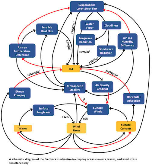
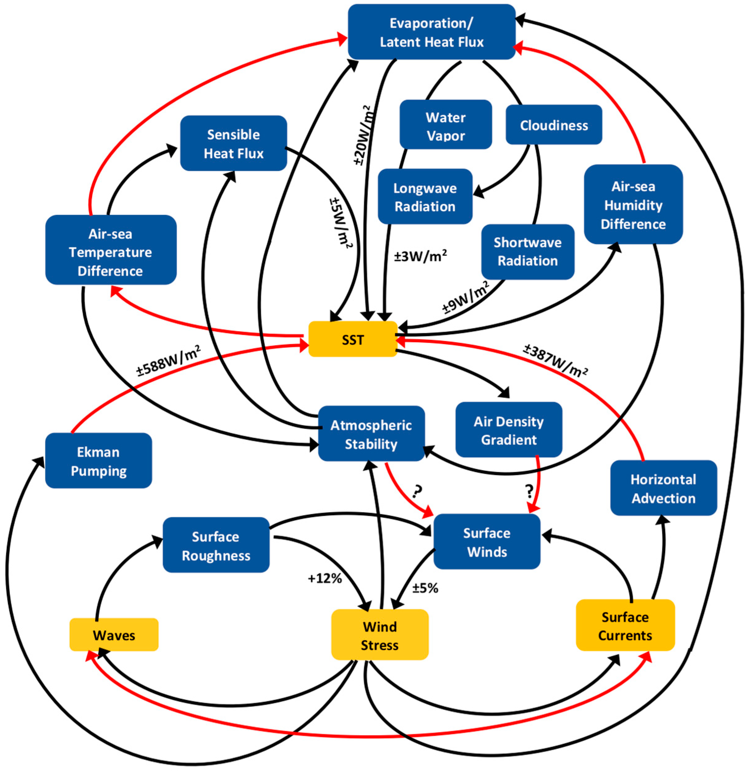
4.2. Feedback Processes

Here, we summarize the feedback processes (Figure 15) that happened in the upper ocean and MABL and provide quantitative impacts based on the difference of the WAV_CUR simulation minus the CRL simulation. These differences emphasize the changes in variables and processes relative to the most common ocean/atmosphere coupling. We also indicate which process is dominant under what conditions. For surface current and wind stress coupling, the ocean surface currents modify the wind stress by 5% over the Gulf Stream by changing the wind shear in the MABL. For waves and wind stress coupling, waves increase the wind stress by 12% over the Gulf Steam by increasing the surface roughness. Changes of wind stress and its curl have a substantial impact on the horizontal current-advection patterns and vertical velocity of Ekman pumping in the upper ocean. Differential horizontal advection and vertical entrainment are two dominant processes that lead to considerable SST change in the Gulf Stream. Since SST is coupled to the MABL, the warming/cooling of SST changes the air temperature and, therefore, changes the pressure gradient near the surface as well as the turbulent vertical mixing, which feeds back to the surface wind. In this study, we find that the contribution of the SST induced surface pressure gradient and the vertical mixing to surface wind change is comparable. However, this result is highly dependent on the surface schemes that we choose. Therefore, more experiments using carefully selected surface roughness schemes are needed to support this conclusion. For surface roughness parameterizations that include sea state, the dependence of the wave model on winds needs to be examined, as 10 meter winds have been shown (Figure 7) to lack the large changes in winds, and the associated changes in stress, at lower heights. SST also influences saturation vapor pressure and boundary-layer stability over the ocean surface, which changes the evaporation over the ocean’s surface. This evaporation change can further impact precipitation and cloud formation/radiation in the atmosphere. Wind stress change impacts the response pattern of waves and surface currents. In the wave–current–stress coupling experiment, current-induced surface roughness and near-surface wind changes play a dominant role in the sea-state response.

4.3. Importance of Horizontal Resolution

The sensitivity of the curl of wind stress on the current is highly dependent on model’s horizontal resolution. Similar to the coupling between the SST gradients and wind described above, we examine the dependence of the curl on the crosswind component of the current gradient (Figure 16). In these examples, the curl is calculated through a line integral approach [74] for roughly circular shapes. This approach allows curls to be calculated on shapes with diameters that are integer multiples of the grid spacing. We calculate curls on a scale of 10, 30, and 60 km, and show these curls against the cross wind current gradient (Figure 16a–c). The 10 km case is analogous to 3 to 5 km grid spacing, which we hope to see in future scatterometers. The 30 km case is analogous to 10 to 15 km spacing, which is similar to most current scatterometer products. The 60 km case is analogous to 20 to 30 km grid spacing, which is similar to earlier versions of Quick Scatteromenter (QuikSCAT) and Advanced Scatterometer (ASCAT-A) products. The resulting slope of vorticity as a function of the cross wind component of the gradient of the surface current depends on the resolution of the curl. However, there is a modest, and non-negligible, reduction in the slope of the 30 km resolution curls relative to the 10 km resolution curls. There is a drastic reduction of slope for the 60 km case. The actual resolution of the scatterometer products is coarser than their grid spacing. Thus, we recommend against comparing modelled curls to observed curls. The sensitivity to resolution is intuitive because a change in a vector component over a small distance results in a larger curl, rather than an identical change over a larger distance. However, the physical implications are much more interesting. This result indicates that areas with strong gradients in the surface current will have a much larger Ekman motion than would be expected based on coarse resolution models. This strong curl plays a large role in the energy budgets mentioned in the prior section.

5. Comparison of Model and Observations

Our validation focuses on the alteration of a stress-related variable across the Gulf Stream. Ideally, we would validate the curl of stress on a 10 km scale, but that is not practical for a month of comparisons with ASCAT data. With a scatterometer object resolution of roughly 20 km, the sharp features at the edge of the model’s Gulf Stream will be blurred. However, we will be able to assess the stress over the Gulf Stream, as well as the stress to the North and South of the Gulf Stream. One month of ASCAT-A observations (51 overpasses) is used in this comparison to model the output at the times and locations of the overpasses. Examples of the overpass coverage are shown in Figure 17. Recall that scatterometers measure equivalent neutral winds [75,76,77], which are winds that can be used to correctly calculate stress using air density and neutral drag coefficients. Equivalent neutral winds are extremely well calibrated [78], but researchers have recently questioned the impact of different stress parameterizations on this calibration. Equivalent neutral winds are determined by using Equation (2) to find a friction velocity and roughness length consistent with observations of the air–sea differences in velocity, temperature, and humidity. The values of u_∗ and z_o are used in (2), assuming the stability term is zero, along with a height of 10 m to determine a wind speed relative to a stationary surface U_EN(10).

The impact of stress parameterization on validation is small because the validation process is dependent on an adjustment from the observed height to the standard height of 10 m. Observations are typically at heights (z_B) of 5 m and occasionally higher for some buoys and all ships:

$${\overrightarrow{U}}_{EN}\left(10\right)-{\overrightarrow{U}}_{EN}\left(z_B\right)=\overrightarrow{\frac{u_{*}}{k}}\left[\ln \left(\frac{10}{z_0}\right)-\ln \left(\frac{z_B}{z_0}\right)\right]=\overrightarrow{\frac{u_{*}}{k}}\left[\ln \left(\frac{10}{z_B}\right)\right],$$

(18)

The value of 10/z_B is rarely larger than 2.5, so ln(10/z_B) is usually between 0.92 and 1.0 for buoys. This results in a change of u_∗/k < 10%. The friction velocity is roughly 4% to 5% of the wind speed for neutral conditions, indicating that height adjustment changes the observations by about 0.1 U_EN. A 10% error in u_∗ results in only a 1% error in U_EN(10). There are usually small differences between friction velocities from Equation (8) and a parameterization similar to that used for scatterometer calibration [11]. It would take a very large error in friction velocity to cause a large bias in calibration, indicating that we have good cause to trust that stress parameterization has little impact on scatterometer calibrations, at least for near neutral conditions.

The impact of using different roughness length parameterizations has been examined for non-neutral conditions [77], but the roughness length parameterization [48] used in this study was not included in that evaluation. Kara et al. [77] found little difference between flux models that used a Charnock-like dependence of roughness length on gravity waves, with roughness length proportional to the square of the friction velocity. However, there were substantial stability-related differences in comparison to the models without roughness length dependent on friction velocity. Stability-related differences in U_EN(10) were on the scale of a few tenths of an ms⁻¹, with rare large systematic differences at about 0.5 ms⁻¹. We can anticipate these stability-related differences with the parameterizations used in this study.

We compared average cross sections from the ASCAT equivalent neutral winds to both the model winds (Figure 18a) and our model winds converted to equivalent neutral winds using the roughness length dependence normally used to calibrate scatterometer winds [76] (Figure 18b). The black dotted line in these images is the composite ASCAT wind speed, and the colored lines are the winds from the four model runs. The overpasses are averaged, with zero being the center of the Gulf Stream, negative distances to the South of the Gulf Stream, and positive differences to the North. It is clear that the accounting for sea state causes large changes in the wind. There are many other sea state dependent parameterizations, which have substantial differences in their dependence on wave characteristics [11,27,49,50]. These other parameterizations should be investigated in future studies.

The adjustment of model winds to equivalent neural winds is critical to compare model winds with scatterometer winds, as seen in Figure 18. However, there are clearly remaining inconsistencies well South of the Gulf Stream. These differences might be due to a misplaced eddy, or they could indicate problems with the physics in the coupled model (e.g., errors in surface flux parameterization, a vertical resolution that is too coarse, or perhaps incorrect vertical mixing). Incorrectly comparing the scatterometer U_EN(10) to model U(10) would suggest that the control or the CUR model runs are more consistent with observations. Comparing it to model U_EN(10) indicates a better fit to the WAV or WAV_CUR model runs, but also more closely clusters the lines for all the model runs, suggesting that the surface stress in the different model runs is more similar than would be expected from the winds alone. Even with the equivalent neutral winds, there is a poor fit for distances more than 100 km south of the Gulf Stream. Accounting for the stability-related changes in the conversion from U(10) to U_EN(10) has a very large impact in the lower wind speed region south of the Gulf Stream. The remaining differences suggest that the coupled model does not capture the full extent of this stability related adjustment: there are errors either in the air–sea temperature difference or in the roughness length.

A point of concern with the above comparison is that the roughness length parameterization used to calibrate scatterometers [76] differs substantially from the roughness length parameterization used in the wave dependent modeling studies [48]. Stresses from Liu and Tang [76] are qualitatively and quantitatively similar to stresses from the COARE 3.0 parameterization used in the control and CUR experiments. However, the model results with CUR parameterization are not a good fit for the ASCAT observations. This suggests that either (1) the wave dependent stress (and hence the roughness length) is inconsistent with satellite observations, or (2) that model inputs (air temperature, sea surface temperature, or surface relative wind speed) to the stress parameterization cause substantial errors. We examine the first suggestion by converting to U_EN(10) using a roughness length parameterization [11] that leads to similar stresses for wind driven waves in near neutral conditions (Figure 16c). This model has a much larger value for Charnock’s constant (a in Equation (6) equals 0.035 rather than 0.011) but was tuned with a wind speed reduced by the wave induced surface motion (Stokes drift). That is, the stress is determined from a wave-adjusted wind shear: ${\overrightarrow{U}}_{10}-{\overrightarrow{U}}_{cur}-0.8{\overrightarrow{U}}_{Stokes}$. Here, we ignore the wave related adjustment and demonstrate the relative lack of importance of the value of Charnock’s constant in comparison to including a Charnock-like dependency on stress. The only other difference in the parameterization is the additional roughness due to capillary waves, which slightly increases the stress for wind speeds from approximately 1.8 to 5 ms⁻¹, which is well below the average wind speeds (Figure 18). Values of U_EN(10) determined to have a greater roughness length (Figure 18c) are substantially lower than those in Figure 18b, indicating that either a smaller roughness length is needed (which is contrary to wave tank and field observations) or that the stability related adjustment of the model’s U_EN(10) is in error in a manner that underestimates the value (as argued above). Therefore, we conclude that (1) the model’s biases south of the Gulf Stream are likely related to air–sea temperature differences, and (2) future studies should use the same parameterizations for surface roughness in the coupled model and the adjustment of model winds to equivalent neutral winds. Further work will be required to examine alternative wave dependent parameterizations of stress (or roughness length) that have a Charnock-like dependency friction velocity. While this study demonstrates that considerably more work is required to improve parameterizations and physical processes related to air–sea coupling, the more important point is that satellite data can be used to test stress parameterizations in models. Further work should also include observations of air–sea temperature differences.

6. Conclusions

This study provides the first detailed analysis of the oceanic and atmospheric response to the current-stress, wave-stress, and wave-current-stress interaction in the Gulf Stream, using a high-resolution three-way coupled regional modeling system (COAWST), where both the ocean and the atmosphere respond to this coupling. We used a numerical model because observations of the marine and atmospheric boundary layer (MABL) are usually too spare for an observational study. Moreover, the coupled model allows us to examine all the related variables in the MABL, albeit within the constraints of the model parameterization. To evaluate the impact of surface currents and waves on air–sea flux, we performed 1 month long simulations with COAWST over the Gulf Stream by using four different model configurations, which differ in the inclusion of surface currents and sea-state parameters explicitly in the wind stress calculation. The large sensitivity of coupling between the curl of winds and the SST gradient associated with major currents suggests that satellite observations can be used to validate the parameterization of surface stress, although not the curl of stress associated with current gradients. Aircraft observations [79] have sufficient resolution and swath width to address this problem, but validation would require many overpasses. A satellite that measures simultaneous winds, currents and waves would be ideal for improving our understanding of air–sea coupling.

Our results highlight the substantial impact of coupling currents/waves with wind stress on the air–sea flux exchange and ocean upwelling over the Gulf Stream. Two-way coupling of waves and wind stress (WAV) causes wind stress (a 30 day average) increase up to 12% over a 95th percentile of the model domain, and increases over 5% are found in 50% of the model domain. For two-way coupling of surface currents and wind stress (CUR), both positive and negative changes of wind stress (over 5%) are found at the Gulf Stream, with only small changes elsewhere. The pattern of wind stress change in the wave-current-stress coupling experiment (CUR_WAV) is similar to that in the CUR experiment, with over 15% increase of wind stress at the Gulf Stream. The current impact on wind stress cancels out the wave impact outside of the Gulf Stream in the CUR_WAV experiment. Part of the wind stress increase is used to grow waves, which results in larger significant wave heights in the wave-current-stress coupling experiment. In contrast, extra wind stress due to wave-stress coupling (WAV) goes into the ocean, which is associated with a decrease of wave height. By comparing each term in the equation of the log wind profile, we find that current-induced surface roughness and near-surface wind changes (the change in the neutral log-profile) play an important role in the sea-state response to wave–current–stress coupling. This increase in near surface wind speeds, along with wave-current interactions, explains the increase in surface roughness and surface stress.

We attempted to validate the modeled stress through comparison to ASCAT’s equivalent neutral winds. The conversion of the model winds to equivalent neutral winds is a critical step in this comparison, and the resulting equivalent neutral winds are sufficiently dependent on the roughness length parameterization, which is equivalent to a drag coefficient parameterization. The method used in this study to identify the dependency of roughness on sea state is not ideal. The modeled equivalent neutral winds are sensitive to how roughness length depends on friction velocity (and hence a dependence on boundary-layer stability) and on the magnitude of the roughness length. This result indicates that comparisons between modeled equivalent neutral winds and satellite winds can be used to assess stress parameterizations and stress-related feedback in coupled models, paving the way toward improvements in future coupled models.

References

1. Wu, J. Wind-induced drift currents. J. Fluid Mech. 1975, 68, 49–70. [Google Scholar] [CrossRef]
2. Bonekamp, H.; Komen, G.J.; Sterl, A.; Janssen, P.A.E.M.; Taylor, P.K.; Yelland, M.J. Statistical Comparisons of Observed and ECMWF Modeled Open Ocean Surface Drag. J. Phys. Oceanogr. 2002, 32, 1010–1027. [Google Scholar] [CrossRef] [Green Version]
3. Kara, A.B.; Metzger, E.J.; Bourassa, M.A. Ocean current and wave effects on wind stress drag coefficient over the global ocean. Geophys. Res. Lett. 2007, 34, L01604. [Google Scholar] [CrossRef]
4. Fan, Y.; Ginis, I.; Hara, T.; Fan, Y.; Ginis, I.; Hara, T. The Effect of Wind–Wave–Current Interaction on Air–Sea Momentum Fluxes and Ocean Response in Tropical Cyclones. J. Phys. Oceanogr. 2009, 39, 1019–1034. [Google Scholar] [CrossRef]
5. Bourassa, M.A.; Gille, S.T.; Bitz, C.; Carlson, D.; Cerovecki, I.; Clayson, C.A.; Cronin, M.F.; Drennan, W.M.; Fairall, C.W.; Hoffman, R.N.; et al. High-Latitude Ocean and Sea Ice Surface Fluxes: Challenges for Climate Research. Bull. Am. Meteorol. Soc. 2013, 94, 403–423. [Google Scholar] [CrossRef]
6. Seo, H.; Miller, A.J.; Norris, J. Eddy – Wind Interaction in the California Current System: Dynamics and Impacts. J. Phys. Oceanogr. 2016, 46, 439–459. [Google Scholar] [CrossRef]
7. Moore, G.W.K.; Renfrew, I.A. An Assessment of the Surface Turbulent Heat Fluxes from the NCEP—NCAR Reanalysis over the Western Boundary Currents. J. Clim. 2002, 2020–2037. [Google Scholar] [CrossRef]
8. Roberts, J.B.; Robertson, F.R.; Clayson, C.A.; Bosilovich, M.G. Characterization of turbulent latent and sensible heat flux exchange between the atmosphere and ocean in MERRA. J. Clim. 2012, 25, 821–838. [Google Scholar] [CrossRef]
9. Zhang, D.; Cronin, M.F.; Wen, C.; Xue, Y.; Kumar, A.; McClurg, D. Assessing surface heat fluxes in atmospheric reanalyses with a decade of data from the NOAA Kuroshio Extension Observatory. J. Geophys. Res. Ocean. 2016, 121, 6874–6890. [Google Scholar] [CrossRef]
10. Rogers, D.P. Air sea interaction: Connecting the ocean and atmosphere. Rev. Geophys. 1995, 33, 1377–1383. [Google Scholar] [CrossRef]
11. Bourassa, M.A. Satellite-based observations of surface turbulent stress during severe weather. Atmos. Interact. 2006, 2, 35–52. [Google Scholar]
12. Wang, C.; Zhang, L.; Lee, S.-K.; Wu, L.; Mechoso, C.R. A global perspective on CMIP5 climate model biases. Nat. Clim. Chang. 2014, 4, 201–205. [Google Scholar] [CrossRef]
13. Zhang, L.; Zhao, C. Processes and mechanisms for the model SST biases in the North Atlantic and North Pacific: A link with the Atlantic meridional overturning circulation. J. Adv. Model. Earth Syst. 2015, 7, 739–758. [Google Scholar] [CrossRef] [Green Version]
14. Zuidema, P.; Chang, P.; Medeiros, B.; Kirtman, B.P.; Mechoso, R.; Schneider, E.K.; Toniazzo, T.; Richter, I.; Small, R.J.; Bellomo, K.; et al. Challenges and Prospects for Reducing Coupled Climate Model SST Biases in the Eastern Tropical Atlantic and Pacific Oceans: The U.S. CLIVAR Eastern Tropical Oceans Synthesis Working Group. Bull. Am. Meteorol. Soc. 2016, 97, 2305–2328. [Google Scholar] [CrossRef] [Green Version]
15. Kara, A.B.; Wallcraft, A.J.; Metzger, E.J.; Hurlburt, H.E.; Fairall, C.W.; Kara, A.B.; Wallcraft, A.J.; Metzger, E.J.; Hurlburt, H.E.; Fairall, C.W. Wind Stress Drag Coefficient over the Global Ocean. J. Clim. 2007, 20, 5856–5864. [Google Scholar] [CrossRef]
16. Cornillon, P.; Park, K.-A. Warm core ring velocities inferred from NSCAT. Geophys. Res. Lett. 2001, 28, 575–578. [Google Scholar] [CrossRef]
17. Kelly, K.A.; Dickinson, S.; McPhaden, M.J.; Johnson, G.C. Ocean currents evident in satellite wind data. Geophys. Res. Lett. 2001, 28, 2469–2472. [Google Scholar] [CrossRef]
18. Chelton, D.B.; Schlax, M.G.; Freilich, M.H.; Milliff, R.F. Satellite Measurements Reveal Persistent Small-Scale Features in Ocean Winds. Science 2004, 303, 978–983. [Google Scholar] [CrossRef] [Green Version]
19. Park, K.A.; Cornillon, P.; Codiga, D.L. Modification of surface winds near ocean fronts: Effects of Gulf Stream rings on scatterometer (QuikSCAT, NSCAT) wind observations. J. Geophys. Res. Ocean. 2006, 111, C03032. [Google Scholar] [CrossRef]
20. Gaube, P.; Chelton, D.B.; Samelson, R.M.; Schlax, M.G.; O’Neill, L.W. Satellite Observations of Mesoscale Eddy-Induced Ekman Pumping. J. Phys. Oceanogr. 2015, 45, 104–132. [Google Scholar] [CrossRef]
21. Dawe, J.T.; Thompson, L.A. Effect of ocean surface currents on wind stress, heat flux, and wind power input to the ocean. Geophys. Res. Lett. 2006, 33, L09604. [Google Scholar] [CrossRef]
22. Janssen, P.A.E.M. Wave-Induced Stress and the Drag of Air Flow over Sea Waves. J. Phys. Oceanogr. 1989, 19, 745–754. [Google Scholar] [CrossRef] [Green Version]
23. Brown, R.A. Surface Fluxes and Remote Sensing of Air–Sea Interactions. In Surface Waves and Fluxes; Springer: Dordrecht, The Netherlands, 1990; pp. 7–27. [Google Scholar]
24. Komen, G.; Janssen, P.A.E.M.; Makin, V.; Oost, W. On the sea state dependence of the Charnock parameter. Glob. Atmos. Ocean Syst. 1998, 5, 367–388. [Google Scholar]
25. Desjardins, S.; Mailhot, J.; Lalbeharry, R.; Desjardins, S.; Mailhot, J.; Lalbeharry, R. Examination of the Impact of a Coupled Atmospheric and Ocean Wave System. Part I: Atmospheric Aspects. J. Phys. Oceanogr. 2000, 30, 385–401. [Google Scholar] [CrossRef]
26. Lalbeharry, R.; Mailhot, J.; Desjardins, S.; Wilson, L.; Lalbeharry, R.; Mailhot, J.; Desjardins, S.; Wilson, L. Examination of the Impact of a Coupled Atmospheric and Ocean Wave System. Part II: Ocean Wave Aspects. J. Phys. Oceanogr. 2000, 30, 402–415. [Google Scholar] [CrossRef]
27. Drennan, W.M.; Taylor, P.K.; Yelland, M.J.; Drennan, W.M.; Taylor, P.K.; Yelland, M.J. Parameterizing the Sea Surface Roughness. J. Phys. Oceanogr. 2005, 35, 835–848. [Google Scholar] [CrossRef]
28. Smith, S.D.; Anderson, R.J.; Oost, W.A.; Kraan, C.; Maat, N.; De Cosmo, J.; Katsaros, K.B.; Davidson, K.L.; Bumke, K.; Hasse, L.; et al. Sea surface wind stress and drag coefficients: The hexos results. Boundary-Layer Meteorol. 1992, 60, 109–142. [Google Scholar] [CrossRef] [Green Version]
29. Powell, M.D.; Vickery, P.J.; Reinhold, T.A. Reduced drag coefficient for high wind speeds in tropical cyclones. Nature 2003, 422, 279–283. [Google Scholar] [CrossRef]
30. Moon, I.-J.; Hara, T.; Ginis, I.; Belcher, S.E.; Tolman, H.L.; Moon, I.-J.; Hara, T.; Ginis, I.; Belcher, S.E.; Tolman, H.L. Effect of Surface Waves on Air–Sea Momentum Exchange. Part I: Effect of Mature and Growing Seas. J. Atmos. Sci. 2004, 61, 2321–2333. [Google Scholar] [CrossRef]
31. Vogelzang, J.; Stoffelen, A. ASCAT Ultrahigh-Resolution Wind Products on Optimized Grids. IEEE J. Sel. Top. Appl. Earth Obs. Remote Sens. 2017, 10, 2332–2339. [Google Scholar] [CrossRef]
32. Bourassa, M.A.; Stoffelen, A.; Bonekamp, H.; Chang, P.; Chelton, D.B.; Courtney, J.; Edson, R.; Figa, J.; He, Y.; Hersbach, H.; et al. Remotely Sensed Winds and Wind Stresses for Marine Forecasting and Ocean Modeling. Front. Mar. Sci. 2018, Submitted. [Google Scholar]
33. Bourassa, M.; Gille, S.; Jackson, D.; Roberts, J.B.; Wick, G. Ocean Winds and Turbulent Air–Sea Fluxes Inferred From Remote Sensing. Oceanography 2010, 23, 36–51. [Google Scholar] [CrossRef]
34. Warner, J.C.; Armstrong, B.; He, R.; Zambon, J.B. Development of a Coupled Ocean-Atmosphere-Wave-Sediment Transport (COAWST) Modeling System. Ocean Model. 2010, 35, 230–244. [Google Scholar] [CrossRef]
35. Olabarrieta, M.; Warner, J.C.; Kumar, N. Wave-current interaction in Willapa Bay. J. Geophys. Res. 2011, 116, C12014. [Google Scholar] [CrossRef]
36. Olabarrieta, M.; Warner, J.C.; Armstrong, B.; Zambon, J.B.; He, R. Ocean–atmosphere dynamics during Hurricane Ida and Nor’Ida: An application of the coupled ocean–atmosphere–wave–sediment transport (COAWST) modeling system. Ocean Model. 2012, 43, 112–137. [Google Scholar] [CrossRef]
37. Nelson, J.; He, R. Effect of the Gulf Stream on winter extratropical cyclone outbreaks. Atmos. Sci. Lett. 2012, 13, 311–316. [Google Scholar] [CrossRef]
38. Phibbs, S.; Toumi, R. Modeled dependence of wind and waves on ocean temperature in tropical cyclones. Geophys. Res. Lett. 2014, 41, 7383–7390. [Google Scholar] [CrossRef]
39. Nicholls, S.D.; Decker, S.G. Impact of Coupling an Ocean Model to WRF Nor’easter Simulations. Mon. Weather Rev. 2015, 143, 4997–5016. [Google Scholar] [CrossRef]
40. Coniglio, M.C.; Correia, J.; Marsh, P.T.; Kong, F. Verification of Convection-Allowing WRF Model Forecasts of the Planetary Boundary Layer Using Sounding Observations. Weather Forecast. 2013, 28, 842–862. [Google Scholar] [CrossRef]
41. Cohen, A.E.; Cavallo, S.M.; Coniglio, M.C.; Brooks, H.E. A Review of Planetary Boundary Layer Parameterization Schemes and Their Sensitivity in Simulating Southeastern U.S. Cold Season Severe Weather Environments. Weather Forecast. 2015, 30, 591–612. [Google Scholar] [CrossRef]
42. Huang, H.-Y.; Hall, A.; Teixeira, J. Evaluation of the WRF PBL Parameterizations for Marine Boundary Layer Clouds: Cumulus and Stratocumulus. Mon. Weather Rev. 2013, 141, 2265–2271. [Google Scholar] [CrossRef] [Green Version]
43. Komen, G.J.; Hasselmann, K.; Hasselmann, K.; Komen, G.J.; Hasselmann, K.; Hasselmann, K. On the Existence of a Fully Developed Wind-Sea Spectrum. J. Phys. Oceanogr. 1984, 14, 1271–1285. [Google Scholar] [CrossRef]
44. Bourassa, M.A.; Vincent, D.G.; Wood, W.L. A Flux Parameterization Including the Effects of Capillary Waves and Sea State. J. Atmos. Sci. 1999, 56, 1123–1139. [Google Scholar] [CrossRef]
45. Fairall, C.W.; Bradley, E.F.; Hare, J.E.; Grachev, A.A.; Edson, J.B.; Fairall, C.W.; Bradley, E.F.; Hare, J.E.; Grachev, A.A.; Edson, J.B. Bulk Parameterization of Air–Sea Fluxes: Updates and Verification for the COARE Algorithm. J. Clim. 2003, 16, 571–591. [Google Scholar] [CrossRef]
46. Edson, J.B.; Jampana, V.; Weller, R.A.; Bigorre, S.P.; Plueddemann, A.J.; Fairall, C.W.; Miller, S.D.; Mahrt, L.; Vickers, D.; Hersbach, H. On the Exchange of Momentum over the Open Ocean. J. Phys. Oceanogr. 2013, 43, 1589–1610. [Google Scholar] [CrossRef] [Green Version]
47. Grachev, A.A.; Fairall, C.W. Dependence of the Monin–Obukhov Stability Parameter on the Bulk Richardson Number over the Ocean. J. Appl. Meteorol. 1997, 36, 406–414. [Google Scholar] [CrossRef]
48. Taylor, P.K.; Yelland, M.J. The Dependence of Sea Surface Roughness on the Height and Steepness of the Waves. J. Phys. Oceanogr. 2001, 31, 572–590. [Google Scholar] [CrossRef] [Green Version]
49. Oost, W.A.; Komen, G.J.; Jacobs, C.M.J.; Van Oort, C. New evidence for a relation between wind stress and wave age from measurements during ASGAMAGE. Boundary-Layer Meteorol. 2002, 103, 409–438. [Google Scholar] [CrossRef]
50. Hsu, S.A. A Dynamic Roughness Equation and Its Application to Wind Stress Determination at the Air–Sea Interface. J. Phys. Oceanogr. 1974, 4, 116–120. [Google Scholar] [CrossRef]
51. Kain, J.S. The Kain–Fritsch Convective Parameterization: An Update. J. Appl. Meteorol. 2004, 43, 170–181. [Google Scholar] [CrossRef]
52. Iacono, M.J.; Delamere, J.S.; Mlawer, E.J.; Shephard, M.W.; Clough, S.A.; Collins, W.D. Radiative forcing by long-lived greenhouse gases: Calculations with the AER radiative transfer models. J. Geophys. Res. 2008, 113, D13103. [Google Scholar] [CrossRef]
53. Haidvogel, D.B.; Beckmann, A. Numerical Ocean Circulation Modeling; Series on Environmental Science and Management; Imperial College Press: London, UK, 1999. [Google Scholar]
54. Booij, N.; Ris, R.C.; Holthuijsen, L.H. A third-generation wave model for coastal regions: 1. Model description and validation. J. Geophys. Res. Ocean. 1999, 104, 7649–7666. [Google Scholar] [CrossRef] [Green Version]
55. Settelmaier, J. Gibbs, a Simulating Waves Nearshore (SWAN) modeling efforts at the National Weather Service (NWS) Southern Region (SR) coastal Weather Forecast Offices (WFOs). In Proceedings of the 91st AMS Annual Meeting, Seattle, WA, USA, 22–28 January 2011; pp. 1–14. [Google Scholar]
56. Chelton, D.B.; Schlax, M.G.; Samelson, R.M. Summertime Coupling between Sea Surface Temperature and Wind Stress in the California Current System. J. Phys. Oceanogr. 2007, 37, 495–517. [Google Scholar] [CrossRef]
57. O’Neill, L.W.; Esbensen, S.K.; Thum, N.; Samelson, R.M.; Chelton, D.B. Dynamical analysis of the boundary layer and surface wind responses to mesoscale SST perturbations. J. Clim. 2010, 23, 559–581. [Google Scholar] [CrossRef]
58. Schneider, N.; Qiu, B. The Atmospheric Response to Weak Sea Surface Temperature Fronts*. J. Atmos. Sci. 2015, 72, 3356–3377. [Google Scholar] [CrossRef] [Green Version]
59. O’Neill, L.W. Wind speed and stability effects on coupling between surface wind stress and SST observed from buoys and satellite. J. Clim. 2012, 25, 1544–1569. [Google Scholar] [CrossRef]
60. Song, Q.; Chelton, D.B.; Esbensen, S.K.; Thum, N.; O’Neill, L.W. Coupling between sea surface temperature and low-level winds in mesoscale numerical models. J. Clim. 2009, 22, 146–164. [Google Scholar]
61. Chelton, D.B.; Xie, S.-P. Coupled Ocean-Atmosphere Interaction at Oceanic Mesoscales. Oceanography 2010, 23, 52–69. [Google Scholar] [CrossRef]
62. Holthuijsen, L.H.; Tolman, H.L. Effects of the Gulf Stream on ocean waves. J. Geophys. Res. Ocean. 1991, 96, 12755–12771. [Google Scholar] [CrossRef]
63. Kenyon, K.E.; Sheres, D.; Kenyon, K.E.; Sheres, D. Wave Force on an Ocean Current. J. Phys. Oceanogr. 2006, 36, 212–221. [Google Scholar] [CrossRef]
64. Caniaux, G.; Planton, S. A three-dimensional ocean mesoscale simulation using data from the SEMAPHORE eperiment: Mixed layer heat Budget. J. Geophys. Res. 1998, 103, 25081–25099. [Google Scholar] [CrossRef]
65. Stevenson, J.W.; Niiler, P.P. Upper Ocean Heat Budget During the Hawaii−to−Tahiti Shuttle Experiment. J. Phys. Oceanogr. 1983, 13, 1894–1907. [Google Scholar] [CrossRef]
66. Kara, A.B.; Rochford, P.A.; Hurlburt, H.E. Mixed layer depth variability and barrier layer formation over the North Pacific Ocean. J. Geophys. Res. Ocean. 2000, 105, 16783–16801. [Google Scholar] [CrossRef] [Green Version]
67. Kara, A.B.; Rochford, P.A.; Hurlburt, H.E. An optimal definition for ocean mixed layer depth. J. Geophys. Res. 2000, 105, 16803–16821. [Google Scholar] [CrossRef]
68. Shchepetkin, A.F.; Mcwilliams, J.C. Quasi-Monotone Advection Schemes Based on Explicit Locally Adaptive Dissipation. Mon. Wea. Rev. 1998, 126, 1541–1580. [Google Scholar] [CrossRef]
69. Wai, M.M.-K.; Stage, S.A. Dynamical analyses of marine atmospheric boundary layer structure near the Gulf Stream oceanic front. Q. J. R. Meteorol. Soc. 1989, 115, 29–44. [Google Scholar] [CrossRef]
70. Wallace, J.M.; Mitchell, T.P.; Deser, C. The Influence of Sea-Surface Temperature on Surface Wind in the Eastern Equatorial Pacific: Seasonal and Interannual Variability. J. Clim. 1989, 2, 1492–1499. [Google Scholar] [CrossRef]
71. Small, R.J.; Xie, S.-P.; Wang, Y.; Esbensen, S.K.; Vickers, D. Numerical Simulation of Boundary Layer Structure and Cross-Equatorial Flow in the Eastern Pacific. J. Atmos. Sci. 2005, 62, 1812–1830. [Google Scholar] [CrossRef]
72. Shin, H.H.; Hong, S.-Y.; Dudhia, J. Impacts of the Lowest Model Level Height on the Performance of Planetary Boundary Layer Parameterizations. Mon. Weather Rev. 2012, 140, 664–682. [Google Scholar] [CrossRef]
73. Vélez-Belchí, P.; Tintoré, J. Vertical velocities at an ocean front. Sci. Mar. 2001, 65, 291–300. [Google Scholar] [CrossRef]
74. Bourassa, M.A.; Ford, K.M. Uncertainty in scatterometer-derived vorticity. J. Atmos. Ocean. Technol. 2010, 27, 594–603. [Google Scholar] [CrossRef]
75. Ross, D.B.; Overland, J.; Plerson, W.J.; Cardone, V.J.; McPherson, R.D.; Yu, T.-W. Chapter 4 Oceanic Surface Winds. Adv. Geophys. 1985, 27, 101–140. [Google Scholar]
76. Liu, W.T.; Tang, W. Equivalent Neutral Winds; JPL Publication 96-17, Jet Propulsion Laboratory: Pasadena, USA, 1996. [Google Scholar]
77. Kara, A.B.; Wallcraft, A.J.; Bourassa, M.A. Air–sea stability effects on the 10 m winds over the global ocean: Evaluations of air–sea flux algorithms. J. Geophys. Res. Ocean. 2008, 113, 1–14. [Google Scholar] [CrossRef]
78. Wentz, F.J.; Ricciardulli, L.; Rodriguez, E.; Stiles, B.W.; Bourassa, M.A.; Long, D.G.; Hoffman, R.N.; Stoffelen, A.; Verhoef, A.; O’Neill, L.W.; et al. Evaluating and Extending the Ocean Wind Climate Data Record. IEEE J. Sel. Top. Appl. Earth Obs. Remote Sens. 2017, 10, 2165–2185. [Google Scholar] [CrossRef] [PubMed] [Green Version]
79. Rodríguez, E.; Wineteer, A.; Perkovic-Martin, D.; Gál, T.; Stiles, B.W.; Niamsuwan, N.; Monje, R.R. Estimating Ocean VectorWinds and currents using a Ka-band pencil-beam Doppler Scatterometer. Remote Sens. 2018, 10, 576. [Google Scholar] [CrossRef]
Figure 1. Coupled-Ocean-Atmosphere-Wave-Sediment Transport (COAWST) configuration and exchanged data fields. We modified the COAWST coupling so that WRF can use current-relative wind for stress calculation. SWAN was already designed to use the current relative winds. Our changes are highlighted in red.
Remotesensing 11 01476 g001
Figure 2. The three domains used for the WRF model simulations.
Remotesensing 11 01476 g002
Figure 3. Change of wind stress magnitude (color shaded, N/m2) and vector (black vectors) due to (a) surface currents and wind stress coupling (CUR-CTL), (b) waves and wind stress coupling (WAV-CTL), and (c) three-way coupling of the surface current, waves, and wind stress (CUR_WAV-CTL) averaged over a 30 day period.
Remotesensing 11 01476 g003
Figure 4. Ekman pumping (color shaded, m/day) response to (a) surface currents and wind stress coupling (CUR-CTL), (b) waves and wind stress coupling (WAV-CTL), and (c) three-way coupling of surface current, waves, and wind stress (CUR_WAV-CTL) averaged over a 30 day period.
Remotesensing 11 01476 g004
Figure 5. Binned scatterplots of wind stress curl versus the crosswind component of the sea surface temperature (SST) gradient from (a) CTL, (b) CUR, (c) WAV, and (d) CUR_WAV. The statistics were computed over the region 35.8N–39.2N, 76W–72W using 30 day averaged fields. The error bars represent the standard deviation within each bin. The slope α of the least squares fit line to the binned average is labeled in each plot.
Remotesensing 11 01476 g005
Figure 6. Comparing the 30 day averaged changes of (ac) significant wave height (in meters), (df) wave length (in meters), and (gi) wave slope (hundredths) among current–stress coupling (left panel), wave–stress coupling (middle panel), and three-way coupling (right panel).
Remotesensing 11 01476 g006
Figure 7. Histogram of six hourly differences of current, stability and log terms in the log–wind equation between the CUR_WAV and WAV experiments, emphasizing the impact of the currents. The statistics for (a,b) are computed over strong-current (|Us| > 1 m/s) and weak-current (|Us| < 1 m/s) regions, respectively. Negative currents changes and associated changes in the log profile term and stability term are indicated as dashed lines, and changes associated with positive currents are indicated as solid lines.
Remotesensing 11 01476 g007
Figure 8. The 30 day averaged SST (shaded, °C) and surface current (vectors, m/s) differences between the (a) CUR and CTL, (b) WAV and CTL, (c) CUR_WAV, and CTL experiments. The monthly-averaged SST from the CTL experiment is also plotted as black contours (CI = 1 °C).
Remotesensing 11 01476 g008
Figure 9. The changes in the budget terms: (ac) heat storage; (df) mean horizontal advection; (gi) perturbation horizontal advection; (jm) net surface heat flux; (np) vertical entrainment for current–stress coupling (CUR–CTL, left panel), wave–stress coupling (WAV–CTL, middle panel), and current–wave–stress (CUR_WAV–CTL, right panel) coupling.
Remotesensing 11 01476 g009
Figure 10. The 30 day averaged (ac) latent heat flux and (df) sensible heat flux (color shade, W/m2) change for CUR, WAV, and CUR_WAV experiments. Contours overlaid in (af) are the corresponding differential SST, with solid and dashed contours (contour interval = 0.2 °C) corresponding to positive and negative values, respectively.
Remotesensing 11 01476 g010
Figure 11. Impact histogram how LHF is changed by surface wind shear, air–sea temperature differences, and humidity differences for (a) CUR, (b) WAV, (c) CUR_WAV, and (d) the average of CUR and WAV.
Remotesensing 11 01476 g011
Figure 12. The 30 day averaged 10-m wind (color shaded, m/s) differences between (a) CUR and CTL, (b) WAV and CTL, and (c) CUR_WAV and CTL.
Remotesensing 11 01476 g012
Figure 13. Histograms of 30 day averaged differential vertical mixing (red), horizontal pressure gradient (black), horizontal advection (blue), and Coriolis force terms of PBL momentum budget analysis between (a) CUR and CTL, (b) WAV and CTL, and (c) CUR_WAV and CTL.
Remotesensing 11 01476 g013
Figure 14. 30 day averaged differences of mean (left column) and eddy (right column) components of the wind work between (a,b) CUR and CTL, (c,d) WAV and CTL, and (e,f) CUR_WAV and CTL.
Remotesensing 11 01476 g014
Figure 15. A schematic diagram of the feedback mechanism in coupling ocean currents, waves, and wind stress, simultaneously. All numbers are a median value of 30 days, averaged difference between CUR_WAV and CTL over the Gulf Stream.
Remotesensing 11 01476 g015
Figure 16. Scatter plots of the wind curl versus the gradient of the current perpendicular to the wind vector from the CUR_WAV experiment. The wind curl is calculated on a scale of (a) 10 km, (b) 30 km, and (c) 60 km, respectively. The error bars represent the standard deviation within each bin.
Remotesensing 11 01476 g016
Figure 17. The Advanced Scatterometer (ASCAT) observed wind speed (color shaded) near the Gulf Stream region on 15 October 2012. The wind speed along the backline is selected for comparison with the modeled surface wind.
Remotesensing 11 01476 g017
Figure 18. Comparison of the averaged ASCAT equivalent neutral winds (black dotted) to (a) model winds, (b) model winds converted to neutral winds using the COARE 3.0 roughness length algorithm, and (c) model winds converted to neutral winds using the Bourassa [11] algorithm.
Remotesensing 11 01476 g018