Abstract
Shallow water bathymetry is important for nautical navigation to avoid stranding, as well as for the scientific simulation of high tide and high waves in coastal areas. Although many studies have been conducted on satellite derived bathymetry (SDB), previously used methods basically require supervised data for analysis, and cannot be used to analyze areas that are unreachable by boat or airplane. In this study, a mapping method for shallow water bathymetry was developed, using random forest machine learning and multi-temporal satellite images to create a generalized depth estimation model. A total of 135 Landsat-8 images, and a large amount of training bathymetry data for five areas were analyzed with the Google Earth Engine. The accuracy of SDB was evaluated by comparison with reference bathymetry data. The root mean square error in the final estimated water depth in the five test areas was 1.41 m for depths of 0 to 20 m. The SDB creation system developed in this study is expected to be applicable in various shallow water regions under highly transparent conditions.
1. Introduction
Shallow water bathymetry is important for nautical navigation to avoid stranding, as well as for the scientific simulation of high tide and high waves in coastal areas. However, only a few open databases with a global reach are suitable for this purpose. The main measurement methods for bathymetry that are currently in use include sonar measurement and airborne laser measurement. Sonar measurements from a research vessel can instantaneously measure a width equal to twice the water depth, however this technique is not efficient in shallow water [1], and there is a risk of stranding. Bathymetry measured by an airborne lidar system is called airborne lidar bathymetry (ALB), and is appropriate for use in shallow waters [2]. However, the target area must be in a flight capable area, and the cost of ALB is still extremely high. Thus, insufficient bathymetric data have been collected for coastal areas which cannot be easily accessed by ship and airplane for these measurements.
Another method that is currently in use for bathymetric measurement is depth estimation via remote sensing, using multi-spectral or hyper-spectral sensors. Many studies have been conducted using this method since the 1970s [3,4,5,6,7,8,9,10,11,12,13,14]. The use of satellite images helps to obtain information about areas that are difficult to access by boat or airplane. Depth information obtained by analyzing satellite images is called satellite derived bathymetry (SDB). Following improvements in the spatial resolution of optical sensors, SDB has been the focus of hydrographic associations worldwide [15]. Studies have been conducted using airborne hyper-spectral sensors [4,5,11], however only a few satellites have hyper-spectral sensors with a high spatial resolution suitable for extracting depth information.
With regard to multi-spectral sensors, studies have used satellite images with a high spatial resolution greater than 30 m, such as those of the Landsat, SPOT, IKONOS, and WorldView satellites [3,6,7,8,9,10,12,13,14]. As analysis methods, an empirical method [8] and physics-based semi-empirical methods [3,9] have been developed and used in SDB studies. Although variable bottom-reflectance and variation in the optical properties of the water column impact accurate depth extraction, using several wavelength bands increases the robustness of the depth estimation [9,11]. However, SDB based on multi-spectral sensors still presents problems for practical use.
Previously used methods basically require supervised training data for each satellite image, and SDB cannot be performed using only a satellite image. In practice, the SDB process is inefficient, since the necessity of field surveys for training bathymetry data means that areas that are unreachable by boat or airplane cannot be analyzed. Kanno et al. [12] proposed a generalized predictor based on the method of Lyzenga et al. [9], and validated its accuracy using WorldView-2 images [13]. However, in the study of the Kanno et al., test sites were relatively close to each other, and the water depth was shallow (average depth of 3.27 m), and further validation using variable data is therefore necessary.
To develop a general water depth estimation model, machine learning is also considered to be a useful approach. Data recorded by multi-spectral sensors have multi-dimensional features. Although it is not easy to build a model that explains the relationship between multi-dimensional feature values and water depth under variable observation conditions, machine learning can be used to automatically investigate numerical models and provide an optimal solution.
Random forest (RF) [16] is one of the machine learning methods that is considered suitable for building regression models that relate satellite images to water depth data. RF automatically creates decision trees using the training data of an objective variable (e.g., water depth), and predictor variables (e.g., pixel values of satellite images), and provides as results the mean of the outputs from the trees of the regression model. Compared with previous simple empirical or semi-empirical models, RF can create more flexible and accurate models based on real data [14].
Previous researchers created regression models from only one or a few satellite images, and produced one bathymetry map from one satellite image for each target area [3,6,7,8,9,10,12,13,14]. It is not easy to obtain a satellite image that is free of clouds, waves, and turbidity across an entire area, and the estimated water depth for a target area obtained from a given satellite image may be different to the results obtained from other images. These problems have not yet been adequately discussed or studied. The calculation cost of satellite image analysis has been a considerable drawback in previous analysis environments, and may have prevented further analysis using many satellite images to solve the above problems.
Google LLC (Mountain View, CA, USA) has provided the Google Earth Engine (GEE), a cloud-based geographical information analysis system, including almost 30 years of Landsat data, which permits analysis using many satellite images over a short period of time. In this study, using the GEE, a water depth estimation model was created by RF using many satellite images for five study areas, with the aim of improving the generality of the model. A bathymetry map for a given target site was created by merging SDBs obtained from the analysis of several satellite images using the depth estimation model.
2. Data
Images captured by the Landsat-8 satellite and provided by the United States Geological Survey (USGS) are available on the GEE. This study used Landsat-8/Surface Reflectance (SR) products created by the USGS using Landsat-8 Surface Reflectance Code (LaSRC) [17], which are atmospherically-corrected images.
The models used to relate satellite image data to reference bathymetry data were created using machine learning. The bathymetry data used as reference data are listed in Table 1. The mean sea level was set as the datum level for these data. Data for Hateruma, Japan; Oahu, USA; and Guanica, Puerto Rico, were measured by airborne lidar systems and data of Taketomi, Japan; and Efate, Vanuatu were measured by single-beam sonar systems.

Table 1.
List of reference bathymetry data for five test areas, two in Japan and one each in the USA, Puerto Rico and Vanuatu. The data were measured by airborne lidar systems (CZMIL and Riegl VO-880G) or single-beam sonar systems (HDS-5 and HDS-7) from a research vessel. Bathymetry measured by an airborne lidar system is called airborne lidar bathymetry (ALB). These data were either provided by the Hydrographic and Oceanographic Department (JHOD)/Japan Coast Guard (JCG), National Oceanic and Atmospheric Administration (NOAA) or Yamaguchi University, or were collected by field survey. The stated data accuracy expresses the error at the 95% confidence interval (CI). The data were classified according to the category Zone of Confidence (ZOC) defined by the international Hydrographic Organization (IHO).
The Hateruma data, which were provided by the Hydrographic and Oceanographic Department (JHOD)/Japan Coast Guard (JCG), meet the standards of S-44 order 1 b, published by the International Hydrographic Organization (IHO) [18], and the maximum allowable vertical uncertainty at the 95% confidence level (CL) for reduced depths (z) is expressed by:
The maximum allowable horizontal uncertainty at the 95% CL for reduced depths of order 1 b is 5 m + 5% of depth. The Oahu and Guanica data were provided by the National Oceanic and Atmospheric Administration (NOAA) through an on-line data viewer [19]. The Taketomi data and Efate data were obtained by the HDS-5 (Lowrance, Tulsa, OK, USA) and HDS-7 (Lowrance, Tulsa, OK, USA) systems, respectively, both of which include differential GPS. The depth error at the 95% confidence interval (CI) of the bathymetry measurements obtained by a representative single-beam sonar is ±0.29 m [20], and the positioning error of real-time differential GPS is lower than 5 m at the 95% CI [21]. In Table 1, the data accuracy is classified according to the category Zone of Confidence (ZOC) defined by the IHO [22]. The required position and depth accuracies for each ZOC are listed in Table 2.
Table 2.
Category ZOC defined by the IHO. Both position and depth accuracy express the error at the 95% CI.
Landsat-8/SR images with cloud coverage of less than 20%, and an observation term between April 2013 and August 2018, were collected for the study areas listed in Table 1. Figure 1 shows sample images of the study areas. The numbers of images for each area are listed in Table 3. The total number of scenes was 135. Two Landsat-8/SR images were required to cover the Guanica area, while a single image was sufficient to cover the other areas. Our study areas are considered as areas of highly transparent water. For Case 1 water [23], optical properties are determined primarily by phytoplankton. Chlorophyll-a concentration is provided as a product of ocean color sensors. The average chlorophyll-a concentrations in our study areas were derived from MODIS/Aqua data from 4 January 2003 to 31 December 2018, provided by the National Aeronautics and Space Administration (NASA) Goddard Space Flight Center, and were found to be less than 1.0 mg/m3.
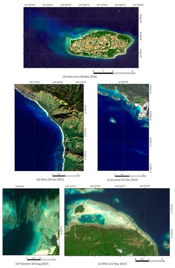
Figure 1.
(a–e) Examples of Landsat-8 images of the study areas.
Table 3.
List of Landsat-8 images.
Bathymetry data (objective variable) and the related pixel values of satellite images (predictor variables) were grouped as one unit of data, and a dataset was created for each satellite image. Here, the dataset is expressed as:
where Ds,j is the dataset for study area s and satellite image j, zi the depth for number i, I is the maximum number of data points in the satellite image, and is the vector value of the reflectance of the satellite image, expressed by Equation (3):
where b is the band number. Bands 1, 2, 3, 4, and 5 were used in our study. Table 4 shows the band number, wavelength, and spatial resolution of the Landsat-8 satellite. The selected band numbers correspond to visible and near-infrared bands with a 30 m spatial resolution. Landsat-8/SR has mask images, including cloud information for each pixel. Pixel data which were judged as cloud were removed from the datasets. The dataset for a study area s (Ds) is expressed as:
where is the number of satellite images for area s and Ns is the number of data points in all the satellite images. The dataset for all five areas (D) was created by binding Ds, as illustrated in Figure 2 and expressed by Equation (5):
where s corresponds to Hateruma, Oahu, Guanica, Taketomi, and Efate, and N is the sum of Ns in all five areas.
Table 4.
Landsat-8 sensor specifications.
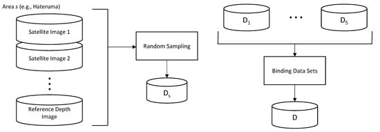
Figure 2.
Process followed for dataset creation. Ds is the dataset for a study area s. The dataset for all five areas () was created by binding Ds.
3. Methods
Our proposed SDB method using machine learning and multi-temporal satellite images follows a three step process (Figure 3). In step 1, the first SDB result is created by an RF analysis of each satellite image. In step 2, a masking process for pixels, including land, cloud, waves, or deep water is applied. In step 3, the final SDB result is produced by merging several SDBs for each target area.
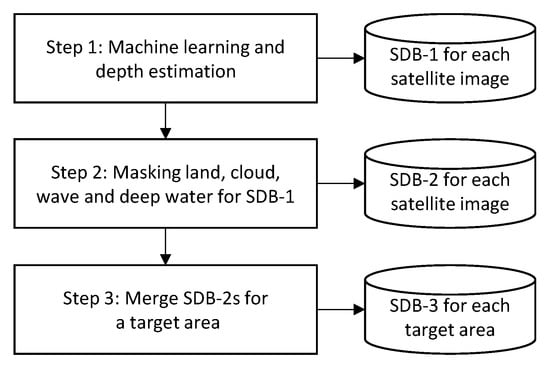
Figure 3.
The three steps of the satellite derived bathymetry (SDB) production process.
3.1. Step 1
The radiance recorded by a satellite sensor can be converted into a reflectance at the top of atmosphere (TOA), which is less influenced by changes in the sun’s irradiance, using Equation (6):
where is the radiance recorded by the band i satellite sensor, is the earth–sun distance, is the average solar spectral irradiance recorded by band i, and is the solar zenith angle. In shallow water, TOA reflectance is expressed as a function of the water depth (z) [3,9]:
where t is a coefficient including the transmittance of the atmosphere and water surface, is the bottom reflectance, Kd is the sum of the diffuse attenuation coefficients for upwelling and downwelling light, g is the coefficient of the optical path length in the water, includes the scattering effect in the atmosphere, and includes the reflected sunlight contribution at the sea surface. To extract water depth information, other variables are needless and obstructive. Landsat-8/SR is an atmospherically-corrected product, and thus the effects of and t are removed. The areas strongly influenced by are masked in step 2.
The RF regression model was selected to build our depth estimation model. All visible Landsat-8 bands were used as predictor variables for RF training. In RF for regression, an arbitrary number of sub-datasets (a value of 10 was empirically set in our study) were extracted by the random sampling from our training dataset. A decision tree for water depth estimation was built for each sub-dataset. To build a tree to precisely and accurately estimate depth, training data should widely and precisely cover the target depth zone. The RF method estimates depth as the mean of the outputs of these decision trees. The RF regression model is flexible, however it is highly dependent upon any training data. It is important that there is a large amount of training data, and that the data cover an objective data distribution. Thus, large amounts and various types of data must be collected to build a general and robust water depth estimation model. The training data should include a slightly wider depth zone than the target zone to obtain information about inapplicable areas. This is the reason that RF modeling is conducted before the masking process in step 2. In this paper, the bathymetry estimated by the predictor for each satellite image in step 1 is called SDB-1.
3.2. Step 2
Land, clouds, boats and the sun glint signal can be masked when using the near-infrared band [9,24]. The surface reflectance of these targets is relatively high, compared with submerged areas, as the attenuation rate in water is high in this wavelength, and the threshold for masking is decided based on statistical values in deep water.
Deep water areas were identified by the visual interpretation of satellite images for each area, and the average and standard deviation of the surface reflectance in near-infrared band (Landsat-8 band 5) was determined for these areas. Using statistical values of the near-infrared band, a threshold () for the masking of upland, terrestrial features, and sun glint was calculated by Equation (8):
where and are the average and standard deviation, respectively, of the surface reflectance in the near-infrared band in deep water areas; and is a coefficient; whose value is set empirically as 10.
Transparency in water is high in the blue-green band wavelength. The statistical values of the blue band (band 2 in Landsat) in deep water were also calculated. Deep water pixels are discriminated by a threshold (), calculated by Equation (9):
where and are the average and standard deviation of surface reflectance in the blue band in deep water, respectively; and is a coefficient, whose value is set to 3 to cover deep water at the 99% CI. The result of applying these masking procedures to SDB-1 is called SDB-2.
3.3. Step 3
The final SDB result, which is called SDB-3, was created by merging the SDB-2 images for the target areas. The median of the SDB-2 values for each pixel was used as the output value. Sea level depends on satellite observation time. Our hypothesis was that a depth relative to the almost mean sea level could be obtained by selecting the median value of the estimated depths derived from multiple satellite images. For each pixel, the number of data points and the standard deviation of SDB-2s were calculated. Pixels with fewer than data points, or whose standard deviation was higher than , were considered as unreliable results. Here, was set as 3 to obtain the minimum value for a calculation of the standard deviation, and was set empirically in our study areas.
3.4. Accuracy Assessment
An accuracy assessment for each SDB step was conducted following the work flow shown in Figure 4. Data were randomly extracted for each area from the created datasets, the maximum number of data points was limited to 20,000, and a new dataset (Ds’) was created for each area. Here, the maximum number is an important parameter, and larger amounts of training data are considered better for machine learning. However, due to limitation of the calculation cost of GEE, 20,000 was almost the maximum number for each area. Then, these data were randomly divided into a training dataset for machine learning (Dts), and an evaluation dataset for accuracy assessment (Des). Regarding the evaluation data, data with water depth of 0 to 20 m depths were the target, and other data were removed. The evaluation datasets for the five areas were created by binding these evaluation datasets as follows:
where Ne is the number of evaluation data in the five areas. The training data should cover a slightly wider depth zone than the evaluation data for practical applications. An RF depth estimation model cannot estimate the depth outside of the depth zone of the training data, therefore it was difficult to judge whether an area was out of range from the estimated result. To distinguish the applicable area, training data with a depth of –5 to 25 m were retained. The training datasets for the five areas were created by binding these training datasets, expressed as:
where Nt is the number of training data in the five areas. The training datasets of all five areas () were used to create a depth estimation model. For comparison, a model was also created using only the training dataset of Hateruma. By applying these models to in the training dataset and the evaluation dataset, assessment data sets for the training dataset and evaluation dataset (Vt and Ve, respectively) were created, as expressed in Equations (12) and (13), respectively:
where is a function of the depth estimation model, and the result corresponds to SDB-1. Training data with a depth of 0 to 20 m were selected for comparison with the evaluation data. Accuracy assessments of SDB-1 for training data and evaluation data were conducted using the Vt and Ve datasets, respectively. Then, by applying mask processing in step 2 using function A(), an assessment dataset was created, which is expressed by Equation (14):
where in the dataset Ve’ corresponds to SDB-2. An accuracy assessment of SDB-2 was conducted using the
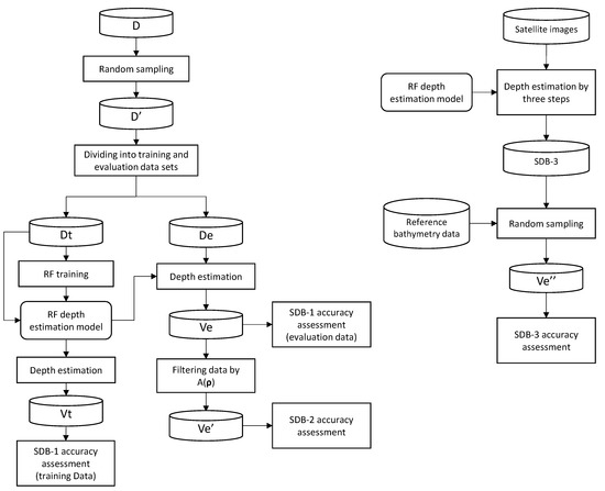
Figure 4.
SDB accuracy assessment process. A new dataset (D’) was created by random sampling from the original dataset (D). D’ was divided into the training dataset (Dt) and an evaluation dataset (De). A random forest (RF) depth estimation model was created using Dt. Vt and Ve are assessment data sets for the training dataset and evaluation dataset of SDB-1, respectively. Ve’ and Ve’’ are assessment data sets for evaluation dataset of SDB-2 and SDB-3, respectively. A() is the function of mask processing.
SDB-3 was created by merging SDB-2s in each pixel, and cannot be created from the dataset Then, SDB-3 was created by applying steps 1–3 to the original satellite images. The pixels were randomly sampled, including reference bathymetry data and SDB-3, and an assessment dataset Ve’’ was created. The maximum number of data points for each area was limited to 10,000 to match the maximum number in the evaluation dataset (). Ve’’ is expressed by Equation (15):
where is SDB-3, and is the number of assessment data.
4. Results
The results of the accuracy assessment for training data from all areas, and for those using data only from Hateruma, are listed in Table 5 and Table 6, respectively. In both tables, the accuracy information, including number of data points (n), root mean square error (RMSE), mean error (ME), and decision coefficient (R2), for SDB-1, SDB-2, and SDB-3 for each area and all areas are listed. In the SDB-1 column, accuracies are listed for both the training data and the evaluation data. Although the water depth zone of the original training data was –5 to 25 m, the training data, with a depth zone of 0 to 20 m, were used for accuracy assessment for comparison with the accuracy of the evaluation data. The accuracy assessment data of SDB-2 were originally the same as the SDB-1 evaluation data, however the number of data points was different due to the masking process. In Table 5 and Table 6, the number of data points decreases to less than two-thirds of the original number for all areas, demonstrating the impact of this process.
Table 5.
Accuracies for satellite derived bathymetry (SDB) when all area data were used for RF training. In the table, the number of data points (n), root mean square error (RMSE), mean error (ME), and decision coefficient (R2) of SDB-1, SDB-2 and SDB-3 for each area and all areas are listed as accuracy information. In the SDB-1 column, accuracies are listed for both training data and evaluation data. Training data for the 0 to 20 m depth zone were used for accuracy assessment, although the depth zone of the original training data was –5 to 25 m. The number of data points in the original data are also listed. The accuracies of SDB-2 and SDB-3 were assessed using the evaluation data separated from the training data used for SDB-1.
Table 6.
Accuracies for SDBs when the Hateruma data were used for training.
In all areas, as shown in Table 4, the RMSE of SDB-1/evaluation data is 2.21 m, 1.67 times larger than the RMSE of the SDB-1/training data (1.32 m). Both the evaluation and training datasets were collected randomly, and there is almost no statistical difference between these two datasets. One of the major reasons for a large difference in errors is the overfitting of the training data in the process of RF learning. Overfitting often occurs in machine learning [25], and it is important to clearly divide evaluation data from training data.
The RMSE of SDB-2 is smaller than that of the SDB-1/evaluation data, and the RMSE of SDB-3 is smaller than that of SDB-2. The total number of training data points was 34,627 across all water depths, and 28,981 in the 0 to 20 m depth zone. The number of data points was different for different study areas, and was larger in Hateruma, Oahu, and Guanica, where ALB bathymetry data are widely available. The number of data points was smaller in Taketomi and Efate, where bathymetry data obtained by single-beam sonar are linearly distributed. However, the effect of the number of data points seems to be small, since the RMSE of the SDB-1/evaluation data in Efate, where the number of data points was smallest, was the third smallest.
As can be seen from Table 5 and Table 6, the RMSE of SDB-3 for Hateruma, when the Hateruma data were used for RF training (Table 6), is lower than it is when all area data were used for RF training (Table 5); however, the difference is only 0.1 m. The RMSE of SDB-3 in all areas when all area data were used for RF training (Table 5) is 0.68 m lower than it is when the Hateruma data were used for RF training (Table 6), which is a relatively large difference. Thus, training using data collected from different areas improves the generality of the RF predictor, and the negative impact on each area seems to be small.
Scatterplots of the SDB and reference bathymetry data for all areas described in Table 5 and Table 6 are shown in Figure 5 and Figure 6, respectively. When SDB data corresponds to the reference bathymetry data, it is located on the y = x line. In Figure 5a, the SDB-1/training data are gathered close to the y = x line, and include few data with a large error. In Figure 5b, the SDB-1/evaluation data are more variable than the training data. The variability of the SDB-2 data (Figure 5c) seems to be smaller than that of the SDB-1/evaluation data. In the plots of SDB-3/evaluation data (Figure 5d), the data points are aggregated close to the y = x line, as are the SDB-1/training data, however the number of outliers seems to be smaller. The plots in Figure 6 look similar to those in Figure 5, however the variability seems to be larger in the plots in Figure 6 than those in Figure 5.
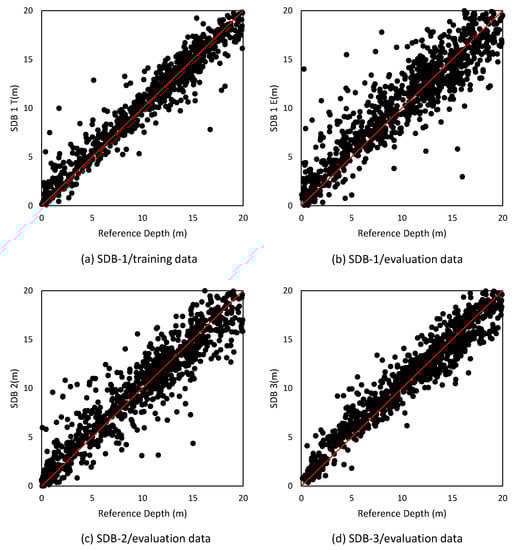
Figure 5.
Scatter plots of SDB versus reference bathymetry data for all areas, when all area data were used for RF training. (a) SDB-1 for training data. (b) SDB-1 for evaluation data. (c) SDB-2 for evaluation data. (d) SDB-3 for evaluation data. In each graph, the x-axis expresses water depth (m) in the reference bathymetry data, and the y-axis expresses water depth (m) in the SDB.
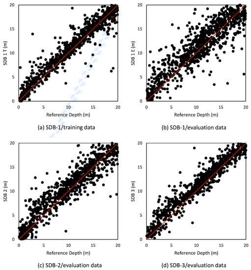
Figure 6.
Scatter plots of SDB versus reference bathymetry data for all areas when the Hateruma area data were used for RF training. (a) SDB-1 for training data. (b) SDB-1 for evaluation data. (c) SDB-2 for evaluation data. (d) SDB-3 for evaluation data. In each graph, the x-axis expresses water depth (m) in the reference bathymetry data, and the y-axis expresses the water depth (m) of SDB.
To determine the relationship between water depth and accuracy, the RMSE and ME for narrower depth zones were also calculated for SDB-3 (Table 5), and the results are shown in Figure 7. From 1 to 19 m in the reference bathymetry h, RMSE and ME were calculated for the range h . The interval of h was 1 m. RMSE was variable, and ranging from 0.83 to 1.91 m. The maximum value of ME was 1.37 m at a depth of 4 m, and ME decreased with the increase of depth after 4 m.
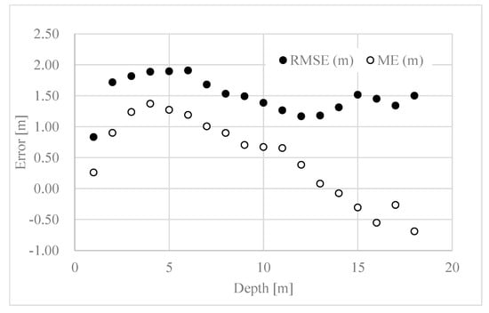
Figure 7.
Error vs. depth for all study areas. The x-axis shows the reference bathymetry (h). The y-axis shows the root-mean-square error (RMSE) and mean error (ME) calculated for the range h. The interval of h was 1 m.
Figure 8, Figure 9, Figure 10, Figure 11 and Figure 12 depict images of SDB and reference bathymetry data in the five study areas. The original reference bathymetry data obtained from ALB and single-beam sonar are point data, however, for comparison with SDB, the data were resampled and converted to images adjusted to the resolution of Landsat-8/SR. Visually, SDB corresponds well with the reference bathymetry images in all areas. The depth was estimated in the SDB, even in places for which there was no data in the reference bathymetry images.
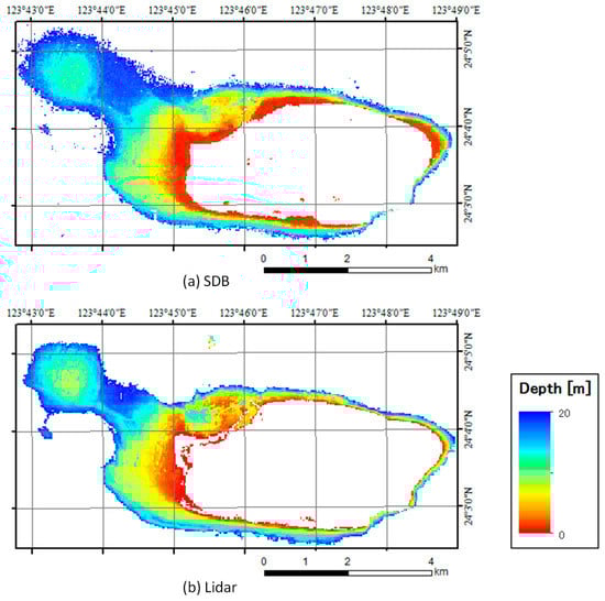
Figure 8.
SDB (a) and reference bathymetry image (b) for Hateruma. In each image, the color scale expresses water depth of 0 to 20 m. White pixels represent areas with no data.
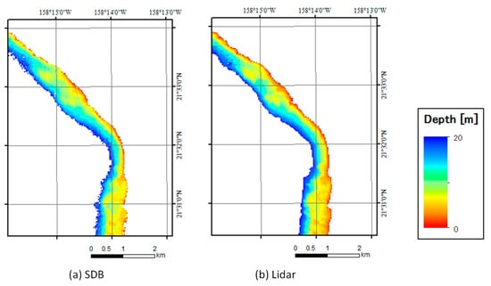
Figure 9.
SDB (a) and reference bathymetry image (b) for Oahu. In each image, the color scale expresses water depths of 0 to 20 m. White pixels represent areas with no data.
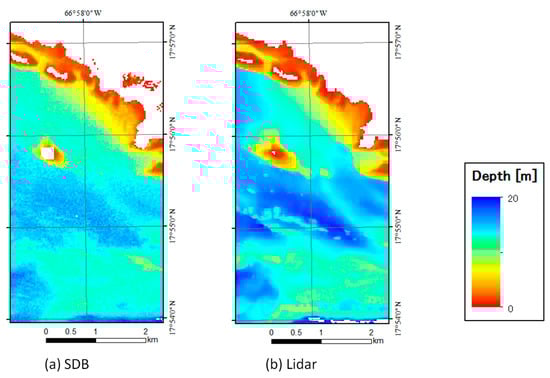
Figure 10.
SDB (a) and reference bathymetry images (b) for Guanica. In each image, the color scale expresses water depths of 0 to 20 m. White pixels represent areas with no data.
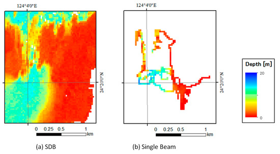
Figure 11.
SDB (a) and reference bathymetry images (b) for Taketomi. In each image, the color scale expresses water depths of 0 to 20 m. White pixels represent areas with no data.
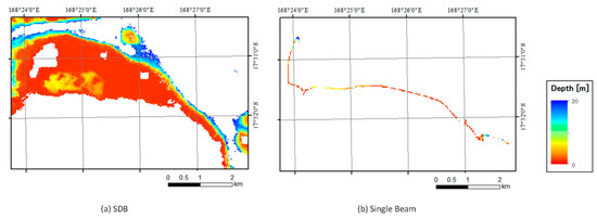
Figure 12.
SDB (a) and reference bathymetry images (b) for Efate. In each image, the color scale expresses water depths of 0 to 20 m. White pixels represent areas with no data.
5. Discussion
A depth estimation model was created employing RF machine learning, using a large amount of training data, and accuracies were evaluated for SDB derived from multiple satellite images. The accuracy of single-scene satellite image analysis corresponds to the accuracy of SDB-2 in our study. The accuracies of SDB-2 were calculated for SDBs derived from more than 10 scenes of satellite images for each study area.
The RMSE of SDB-2 for each study area ranged from 1.77 to 1.97 m and 1.87 m for all areas. These errors are similar to the results obtained for single-scene analysis in previous studies [6,9,13], although conditions were different, and therefore the results cannot be directly compared. The accuracy of SDB was improved by merging multiple SDBs, and RMSE was reduced to 78% (1.41/1.87) in all area assessments. RMSE varied depending on the water depth, however there was no systematic relationship between RMSE and water depth. The observed decreases in ME with increasing water depth indicate that the error due to underestimation increases in deeper water.
Although RMSE and ME were calculated as accuracy indexes in our study, S-44 1b and ZOC, defined by the IHO, are the standards of the maximum allowable error at the 95% CI. When RMSE is and ME is 0, the error range at the 95% CI is , and this range becomes smaller with increasing ME. Then the result has a maximum allowable error of at the 95% CI, when ≤ /1.96 is fulfilled. In our study, the RMSE of the estimated water depth was 1.41 m, and the positioning accuracy of Landsat-8 is 65 m circular error at the 90% CL [26]. These accuracies do not meet the IHO S-44 1b standards. Regarding the ZOC standards, the accuracies of our results meet the ZOC/C standards, which state that the errors for position and water depth are 500 m at 95% CI and 2.00 m + 5% z at 95% CI (where, z is the water depth in meters), respectively. The required accuracies for ZOC/B for position and water depth are 50 m at the 95% CI and 1.00 m + 2 % z at the 95% CI, respectively, and our results do not meet these standards. To meet the standards of S-44 1b or ZOC/B, satellite images with a higher spatial resolution would need to be analyzed, such as those from Sentinel-2 or WorldView-3.
International bathymetry mapping projects include the Seabed 2030 project, a collaborative project between the Nippon Foundation (Minato-ku, Tokyo, Japan) and the General Bathymetric Chart of the Oceans (GEBCO). It aims to create bathymetric map data all over the world with a 100 m mesh size by the year 2030. The SDB maps created in this study have a resolution of 30 m, and contribute to the project for shallow water mapping.
The unique elements of our study include using machine learning and multi-temporal satellite images for water depth estimation. Machine learning has a superior flexibility, and can be used to create suitable models if large amounts of training data are available. Previously, collecting sufficient training data was difficult. Today however, GEE enables efficient analysis of satellite images on a cloud computing system, in which the process of downloading satellite images can be skipped and satellite images can be analyzed directly on the cloud system. Aside from GEE, Amazon Web Services (AWS), operated by Amazon.com, Inc. (Seattle, WA, USA), also provides a satellite image analysis environment on a cloud computing system. Computing cost limits the number of datasets that can be used in GEE. A limited amount of data is a cause of overfitting in RF training. If a larger amount of data is made available by improvements to the analysis environment, and the efficiency of programming for implementation, further increases in the accuracy of SDB will be expected.
There are several other machine learning methods aside from RF. For example, the support vector machine (SVM) method was applied to produce SDB by Misra et al. [27], who achieved a performance that was comparable to the method of Lyzenga et al. [9]. Additionally, deep learning methods, such as convolutional neural networks (CNNs), have produced notable results in many fields [28], and are also considered to be useful for producing SDB.
Only a few studies have focused on the analysis of multi-temporal satellites for water depth estimation. GEE improves the efficiency of the analysis of multi-temporal satellite images. When analyzing a single satellite image, moving objects such as clouds and ships prevent underwater information from being obtained. Figure 13 shows the number of SDB data points created for each pixel in the Hateruma area, and indicates that multiple SDBs help to reduce the amount of missing data. In shallow water between 0 and 20 m in depth, many pixels have about 10 or more data points. Not all of the SDB results are effective; however, unexpected results were also obtained, especially in deep water. In step 3 of our SDB method, the threshold for the number of SDB data points was set to three; however, if more SDB data points are available, choosing a larger number for the threshold may effectively exclude unreliable results. Figure 14 shows the standard deviations of the SDB data points for each pixel in the Hateruma area. The figure indicates that the standard deviation is low for shallow water, and high for water around 20 m in depth. In areas with high standard deviations of SDB, the estimation of water depth is difficult, and such areas could have been removed by the masking based on values of standard deviation. In our study, the threshold value of standard deviation for masking was empirically determined as five, however the proper value may depend upon analysis conditions such as the number of satellite images, the types of satellite sensor, and the environment of the target area.
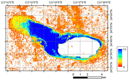
Figure 13.
Number of SDB data points for each pixel in the Hateruma area.
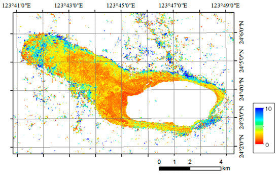
Figure 14.
Standard deviation of SDB data points for each pixel in the Hateruma area.
6. Conclusions
In this study, a new depth estimation method using machine learning and multi-temporal satellite images was proposed with the aim of creating a robust depth estimation model for high-transparency coastal waters. The RMSE of the final SDB products in all five studied areas for water depths of 0 to 20 m was 1.41 m.
GEE was an essential analysis environment to complete this research. Satellite image analysis systems based on cloud computing, such as GEE and AWS, will accelerate researches in many fields which require analysis of machine learning and multi-temporal satellite images.
The SDB production system developed in our study is expected to be applicable to various highly transparent shallow waters regions, which is the advantage of our method compared with traditional bathymetry measurement methods.
One of the problems in the analysis of multi-temporal satellite images for the purpose of water depth estimation is the tide level. We hypothesize that the water depth relative to the almost mean sea level could be obtained by selecting the median value of the estimated water depths derived from multiple satellite images. The validation of this hypothesis, and the improvement of accuracy by compensating for tide effect, are subjects for future study.
The depth estimation model used in this study was constructed using training data from highly transparent water. For less transparent water, another model may have to be built. Further studies including parameters of optical properties of the water column, such as chlorophyll-a, could lead to the improvement of our model.
We expect that the SDB obtained using our proposed method will contribute to various fields that require shallow water bathymetry.
Author Contributions
Conceptualization, T.S.; methodology, T.S.; validation, T.S. and Y.Y.; software, T.S. and Y.Y.; Formal analysis, T.S. and Y.Y.; writing—original draft preparation, T.S.; writing—review and editing, T.S., Y.Y. T.Y. and T.O.; visualization, T.S.; supervision, T.S.; project administration, T.O.; funding acquisition, T.S. and T.O.
Funding
This research was funded by DeSET project of Nippon foundation and Leave a Nest Co., Ltd.
Acknowledgments
The authors would like to thank Hydrographic and Oceanographic Department, Japan Coast Guard and Ariyo Kanno, Yamaguchi University for providing bathymetry data. The authors also thank Yoshimitsu Tajima, University of Tokyo for supporting us to collect bathymetry data in Vanuatu.
Conflicts of Interest
The authors declare no conflict of interest.
References
- Smith, W.; Sandwell, D. Conventional Bathymetry, Bathymetry from Space, and Geodetic Altimetry. Oceanography 2004, 17, 8–23. [Google Scholar] [CrossRef]
- Irish, J.L.; Lillycrop, W.J. Scanning laser mapping of the coastal zone: The SHOALS system. ISPRS J. Photogramm. Remote Sens. 1999, 54, 123–129. [Google Scholar] [CrossRef]
- Lyzenga, D.R. Passive remote-sensing techniques for mapping water depth and Bottom Features. Appl. Opt. 1978, 17, 379–383. [Google Scholar] [CrossRef] [PubMed]
- Lee, Z.; Carder, K.L.; Mobley, C.D.; Steward, R.G.; Patch, J.S. Hyperspectral remote sensing for shallow waters: 1. A semianalytical model. Appl. Opt. 1998, 37, 6329–6338. [Google Scholar] [CrossRef]
- Lee, Z.; Carder, K.L.; Mobley, C.D.; Steward, R.G.; Patch, J.S. Hyperspectral remote sensing for shallow waters: 2. Deriving bottom depth and water properties. Appl. Opt. 1999, 38, 3831–3843. [Google Scholar] [CrossRef] [PubMed]
- Lafon, V.; Froidefond, J.; Lahet, F.; Castaing, P. SPOT shallow water bathymetry of a moderately turbid tidal inlet based on field measurements. Remote Sens. Environ. 2002, 81, 136–148. [Google Scholar] [CrossRef]
- Liceaga-Correa, M.A.; Euan-Avila, J.I. Assessment of coral reef bathymetric mapping using visible Landsat Thematic Mapper data. Int. J. Remote Sens. 2002, 23, 3–14. [Google Scholar] [CrossRef]
- Stumpf, R.P.; Holderied, K.; Sinclair, M. Determination of water depth with high-resolution satellite imagery over variable bottom types. Limnol. Oceanogr. 2003, 48, 547–556. [Google Scholar] [CrossRef]
- Lyzenga, D.R.; Malinas, N.P.; Tanis, F.J. Multispectral bathymetry using a simple physically based algorithm. IEEE Trans. Geosci. Remote Sens. 2006, 44, 2251–2258. [Google Scholar] [CrossRef]
- Kao, H.-M.; Ren, H.; Lee, C.-S.; Chang, C.-P.; Yen, J.-Y.; Lin, T.-H. Determination of shallow water depth using optical satellite images. Int. J. Remote Sens. 2009, 30, 6241–6260. [Google Scholar] [CrossRef]
- Dekker, A.G.; Phinn, S.R.; Anstee, J.; Bissett, P.; Brando, V.E.; Casey, B.; Fearns, P.; Hedley, J.; Klonowski, W.; Lee, Z.P.; et al. Intercomparison of shallow water bathymetry, hydro-optics, and benthos mapping techniques in Australian and Caribbean coastal environments: Intercomparison of shallow water mapping methods. Limnol. Oceanogr.-Meth. 2011, 9, 396–425. [Google Scholar] [CrossRef]
- Kanno, A.; Tanaka, Y. Modified Lyzenga’s Method for Estimating Generalized Coefficients of Satellite-Based Predictor of Shallow Water Depth. IEEE Geosci. Remote Sens. Lett. 2012, 9, 715–719. [Google Scholar] [CrossRef]
- Kanno, A.; Tanaka, Y.; Kurosawa, A.; Sekine, M. Generalized Lyzenga’s predictor of shallow water depth for multispectral satellite imagery. Mar. Geod. 2013, 36, 365–376. [Google Scholar] [CrossRef]
- Manessa, M.D.M.; Kanno, A.; Sekine, M.; Haidar, M.; Yamamoto, K.; Imai, T.; Higuchi, T. Satellite-derived bathymetry using random forest algorithm and worldview-2 Imagery. Geoplan. J. Geomat. Plan. 2016, 3, 117–126. [Google Scholar] [CrossRef]
- Mavraeidopoulos, A.K.; Pallikaris, A.; Oikonomou, E. Satellite Derived Bathymetry (SDB) and Safety of Navigation. Int. Hydrogr. Rev. 2017, 17, 7–20. [Google Scholar]
- Breiman, L. Random Forests. Mach. Learn. 2001, 45, 5–32. [Google Scholar] [CrossRef]
- U.S. Geological Survey. Landsat 8 Surface Reflectance Code (LaSRC) Product Guide 2018. Available online: https://www.usgs.gov/media/files/landsat-8-surface-reflectance-code-lasrc-product-guide (accessed on 20 April 2019).
- International Hygrographic Organization. IHO Standards for Hydrographic Surveys, Special Publication No. 44, 5th ed.; International Hydrographic Bureau: Monaco, Principality of Monaco, 2008. [Google Scholar]
- NOAA Bathymetric Data Viewer. Available online: https://maps.ngdc.noaa.gov/viewers/bathymetry (accessed on 20 April 2019).
- Matsuda, T.; Tababe, K.; Kannda, H. Narrow-multibeam echosounders designed for shallow water. J. Jpn. Soc. Mar. Surv. Technol. 2000, 12, 15–19. [Google Scholar]
- Than, C. Accuracy and Reliability of Various DGPS Approaches. Master’s Thesis, The University of Calgary, Calgary, AB, Canada, May 1996. [Google Scholar]
- International Hygrographic Organization. Supplementary Information for Encording of S-57 Edition 3.1 ENC Data (S-57 Supplement No. 3); International Hydrographic Bureau: Monaco, Principality of Monaco, 2014. [Google Scholar]
- Morel, A.; Prieur, L. Analysis of variations in ocean color1: Ocean color analysis. Limnol. Oceanogr. 1977, 22, 709–722. [Google Scholar] [CrossRef]
- Mishra, D.R.; Narumalani, S.; Rundquist, D.; Lawson, M. High-resolution ocean color remote sensing of benthic habitats: A case study at the Roatan island, Honduras. IEEE Geosci. Remote Sens. 2005, 43, 1592–1604. [Google Scholar] [CrossRef]
- Dietterich, T. Overfitting and undercomputing in machine learning. ACM Comput. Surv. 1995, 27, 326–327. [Google Scholar] [CrossRef]
- Landsat 8 Data Users Handbook. Available online: https://www.usgs.gov/land-resources/nli/landsat/landsat-8-data-users-handbook (accessed on 22 March 2019).
- Misra, A.; Vojinovic, Z.; Ramakrishnan, B.; Luijendijk, A.; Ranasinghe, R. Shallow water bathymetry mapping using Support Vector Machine (SVM) technique and multispectral imagery. Int. J. Remote Sens. 2018, 39, 4431–4450. [Google Scholar] [CrossRef]
- LeCun, Y.; Bengio, Y.; Hinton, G. Deep learning. Nature 2015, 521, 436–444. [Google Scholar] [CrossRef] [PubMed]
© 2019 by the authors. Licensee MDPI, Basel, Switzerland. This article is an open access article distributed under the terms and conditions of the Creative Commons Attribution (CC BY) license (http://creativecommons.org/licenses/by/4.0/).