Article

Mapping Damage-Affected Areas after Natural Hazard Events Using Sentinel-1 Coherence Time Series

Institute for Earth and Environmental Science, University of Potsdam, 14469 Potsdam, Germany
*
Author to whom correspondence should be addressed.
Remote Sens. 2018, 10(8), 1272; https://doi.org/10.3390/rs10081272
Submission received: 30 June 2018 / Revised: 6 August 2018 / Accepted: 8 August 2018 / Published: 13 August 2018

Abstract

:
The emergence of the Sentinel-1A and 1B satellites now offers freely available and widely accessible Synthetic Aperture Radar (SAR) data. Near-global coverage and rapid repeat time (6–12 days) gives Sentinel-1 data the potential to be widely used for monitoring the Earth’s surface. Subtle land-cover and land surface changes can affect the phase and amplitude of the C-band SAR signal, and thus the coherence between two images collected before and after such changes. Analysis of SAR coherence therefore serves as a rapidly deployable and powerful tool to track both seasonal changes and rapid surface disturbances following natural disasters. An advantage of using Sentinel-1 C-band radar data is the ability to easily construct time series of coherence for a region of interest at low cost. In this paper, we propose a new method for Potentially Affected Area (PAA) detection following a natural hazard event. Based on the coherence time series, the proposed method (1) determines the natural variability of coherence within each pixel in the region of interest, accounting for factors such as seasonality and the inherent noise of variable surfaces; and (2) compares pixel-by-pixel syn-event coherence to temporal coherence distributions to determine where statistically significant coherence loss has occurred. The user can determine to what degree the syn-event coherence value (e.g., 1st, 5th percentile of pre-event distribution) constitutes a PAA, and integrate pertinent regional data, such as population density, to rank and prioritise PAAs. We apply the method to two case studies, Sarpol-e, Iran following the 2017 Iran-Iraq earthquake, and a landslide-prone region of NW Argentina, to demonstrate how rapid identification and interpretation of potentially affected areas can be performed shortly following a natural hazard event.

1. Introduction

The emergence of synthetic aperture radar (SAR)-based Earth Observation (EO) satellites over the last decades has led to the development of powerful new methods for monitoring the Earth’s surface. This is particularly true in the case of monitoring and assessing the impacts of natural hazards [1,2,3]. SAR satellites observe the Earth’s surface independent of weather conditions and time of day, as the active radar signal does not depend on daylight and penetrates cloud cover with minimal atmospheric interaction [4]. This is especially an advantage in assessing natural hazards associated with heavy precipitation, such as flooding and rainfall-triggered landslides, debris flows, and mudflows, when persistent cloud-cover may render optical satellite observations of limited use [2]. Interferometric SAR (InSAR) coherence, or the correlation between two images, is a widely used metric derived from SAR images, e.g., [5]. Because coherence loss between two images with a similar spatial footprint collected at different times results from changes at the Earth’s surface, it is a particularly useful metric to map where potential damage has occurred following natural hazard or meteorological events [6,7,8,9].
Mapping potential damage following a natural hazard event is generally performed via a comparison of pre-event and syn-event (i.e., comparison of one SAR image before and one image after the event) coherence images. The resulting map of coherence loss provides a spatial estimate of where damage may have occurred. Coherence studies using this approach for the purpose of surface damage monitoring have typically used the longer-wavelength L-band radar systems (e.g., the Japanese ALOS satellites) [6,10,11], which are less sensitive to surficial changes and partially penetrate through ephemeral and variable surface features such as vegetation cover. The shorter wavelength X-band radar systems (e.g., TerraSAR-X [12] or COSMO-SkyMed [13]) are sensitive SAR systems for urban or vegetation-free areas. However, access to SAR data from current X- and L-band systems is limited by availability and expense, restricting the applicability of SAR coherence estimates of areas affected following a natural hazard and are not easily accessible for continuous monitoring. Furthermore, relying on a single pre-event coherence estimate (i.e., from a single SAR pair) neglects the natural variability in the SAR coherence signal through time for different land covers or climatic regions. This is now changing following the launch in 2014 of the European Space Agency (ESA) Sentinel-1 satellites. The Sentinel-1 satellites are equipped with C-band radar and offer near global coverage with a relatively high repeat time (6–12 days). Sentinel-1 data are freely available as part of the ESA Copernicus program [14,15]. Despite these advantages, however, the C-band radar presents potential challenges for Earth surface observation due to its higher sensitivity to surficial changes and vegetation cover, which can provide a noisier signal, particularly in regions with high or seasonal vegetation coverage.
In this study, we present a method that takes advantage of the high accessibility and high frequency of repeated observations of Sentinel-1 radar for natural hazard monitoring and assessment, while mitigating the inherent noisiness of the C-band radar system. Following previous methods for potential damage mapping, such as the NASA Damage Proxy Map [6] and the Earthquake Damage Visualisation method [11], we compare syn-event coherence related to a natural hazard event to pre-event coherence. However, rather than relying on a single estimate of pre-event coherence, we take advantage of the wealth of Sentinel-1 data to characterise the statistical character of pre-event coherence through time for each pixel.
For the first time, the Sentinel-1 system allows for the construction of large time series and databases of SAR data that may not be financially feasible with costlier commercial satellite systems for many institutions. By constructing a time series of SAR coherence data for a region of interest, we suggest a methodology that focuses on three critical objectives: (1) Deriving a more complete distribution of coherence values through SAR time series analysis for each pixel to decipher more accurately anomalous events; (2) Using this distribution, to identify time periods or seasons most suitable for the detection of anomalous, landscape-changing events; (3) Based on the distribution, to derive different significance levels of coherence thresholds to identify natural hazards. Regions where coherence loss exceeds a given threshold are considered Potentially Affected Areas (PAAs). The threshold for this determination is calculated dynamically from the time series; for example, this can be set as the 5th percentile of the pixel’s coherence distribution.
We apply the method to two independent case studies: the 2017 Mw 7.2 earthquake on the Iran-Iraq border, and in the landslide-prone Quebrada del Toro in the south-central Andes in rural, northwestern Argentina. Additional data, such as settlement locations, population, and/or infrastructure, can be included to assess potential human and economic impacts from natural hazard events and prioritise potentially affected regions. Thus, we present a framework where users can create a rapid assessment of potentially affected areas and employ case-specific information to filter, rank, and interpret the potential damages following a natural hazard event.

2. Methods

2.1. InSAR Coherence Measurements

SAR systems are active radar systems in the microwave spectrum that transmit and receive reflected waves from the Earth’s surface. The SAR signal consists of an amplitude (i.e., return strength) and phase (i.e., phase offset of a sinusoidal wave). Each pixel of a SAR image is a complex number, where the wave is represented by a real and imaginary part corresponding to respective amplitude and phase values, e.g., [16]. In order to compare two SAR scenes and calculate coherence, the scenes need to be precisely aligned to each other, where the secondary scene (date 2) is usually resampled to the primary scene (date 1). We rely on a zero-doppler scene-pair geometry and baselines of Sentinel-1 imagery are generally low (<200 m) and geared toward radar interferometry. The coherence between two SAR images is the normalised complex correlation coefficient,
c o h e r e n c e = s 1 s 2 ( s 1 s 1 s 2 s 2 )
where s1, s2 are the complex pixel values at times t = 1 and t = 2; s* is the complex conjugate of s; and 〈〉 is the ensemble average [5,17]. Coherence is a normalised metric and values range from 0 to 1, where 1 represents perfect coherence, which in reality is rarely observed. Coherence is sensitive to changes to either the phase or amplitude of a pixel. For example, change in surface elevation (e.g., destruction of a building), backscattering properties (e.g., vegetation growth or removal), or the dielectric character of the surface (e.g., wet versus dry soil) will result in coherence loss [17]. Therefore, it is important to note that coherence values result in a spatial and temporal estimate of where and when change has occurred, but cannot constrain the type or rate of change.
We calculated the physiographic coherence between two images using the InSAR Scientific Computing Environment (ISCE) from the NASA Jet Propulsion Laboratory [18,19,20]. SAR images were multi-looked to 30 × 30 m by 12 range, 2 azimuth multi-looking of ~3 × ~20 m data, and topographically corrected using the Shuttle Radar Topography Radar Mission (SRTM) 1-arcsecond (~30 m) global Digital Elevation Model (DEM) [21]. To create the database for a region, coherence was calculated for every adjacent pair in a time series (e.g., date-1 & date-2, date-2 & date 3, …, date-n & date-n + 1) to measure the coherence with the lowest possible temporal baseline.

2.2. Algorithm for Potentially Affected Area Detection

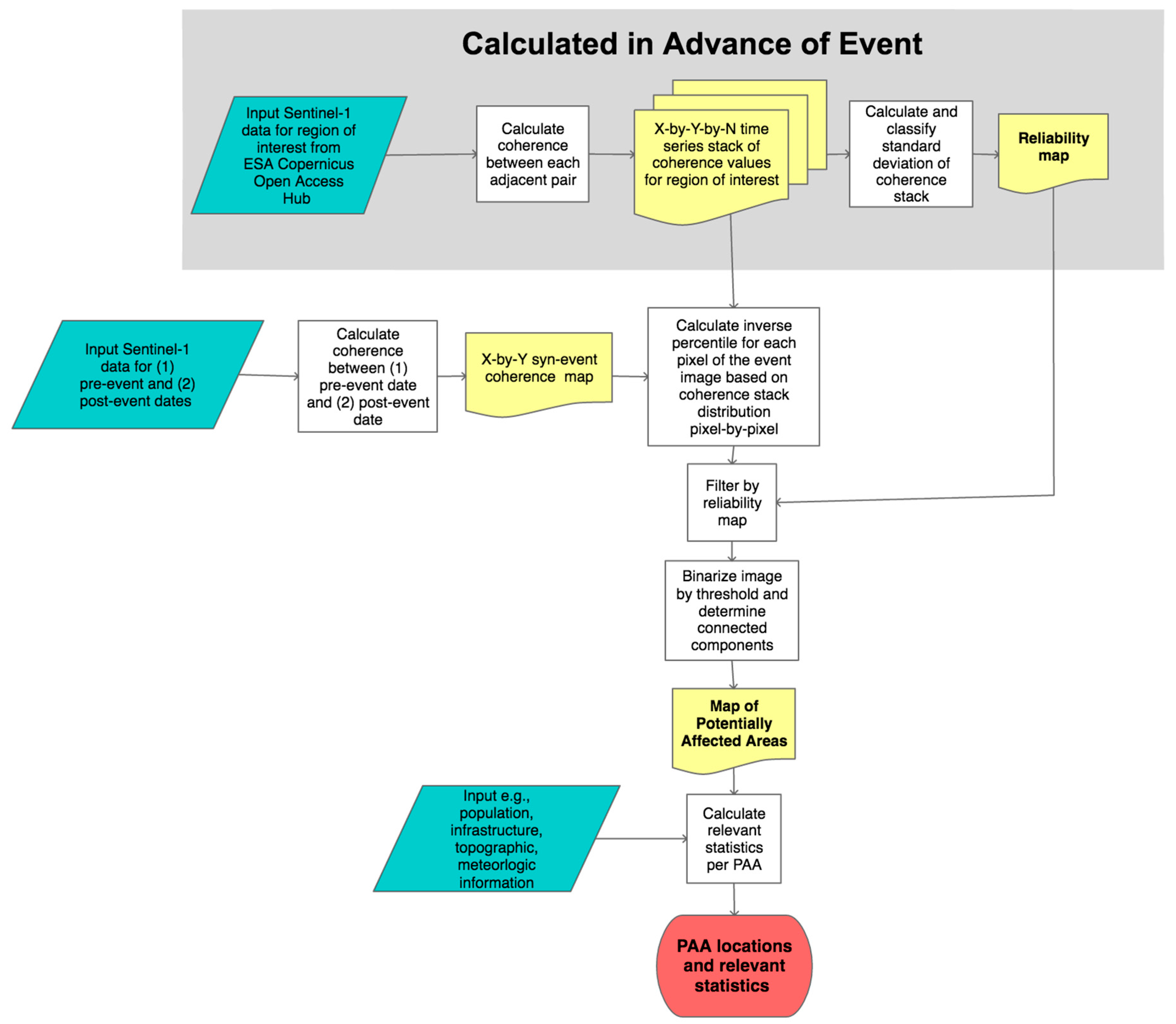
In order to identify Potentially Affected Areas (PAAs) related to a natural hazard event, we construct a simple algorithm using a time series of coherence data, summarised in Figure 1. SAR images for at minimum one year were obtained from the ESA Copernicus Open Access Hub [22] and coherence was calculated using ISCE following the parameters outlined in Section 2.1 above. The coherence values were then amalgamated into a spatially referenced x-by-y-by-n stack, where the spatial dimension is given by x and y and the temporal component by n. This temporal coherence stack is then the basis from which we characterise pixel-by-pixel reliability, as described below, and coherence distributions through time.
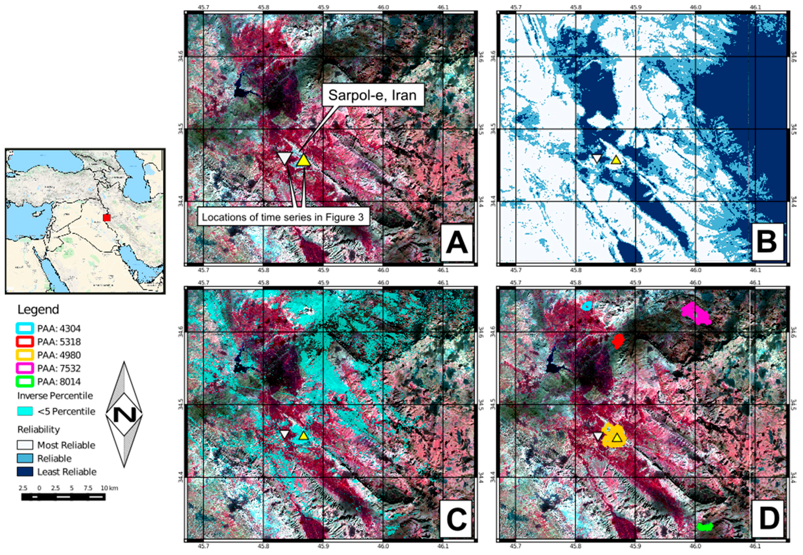
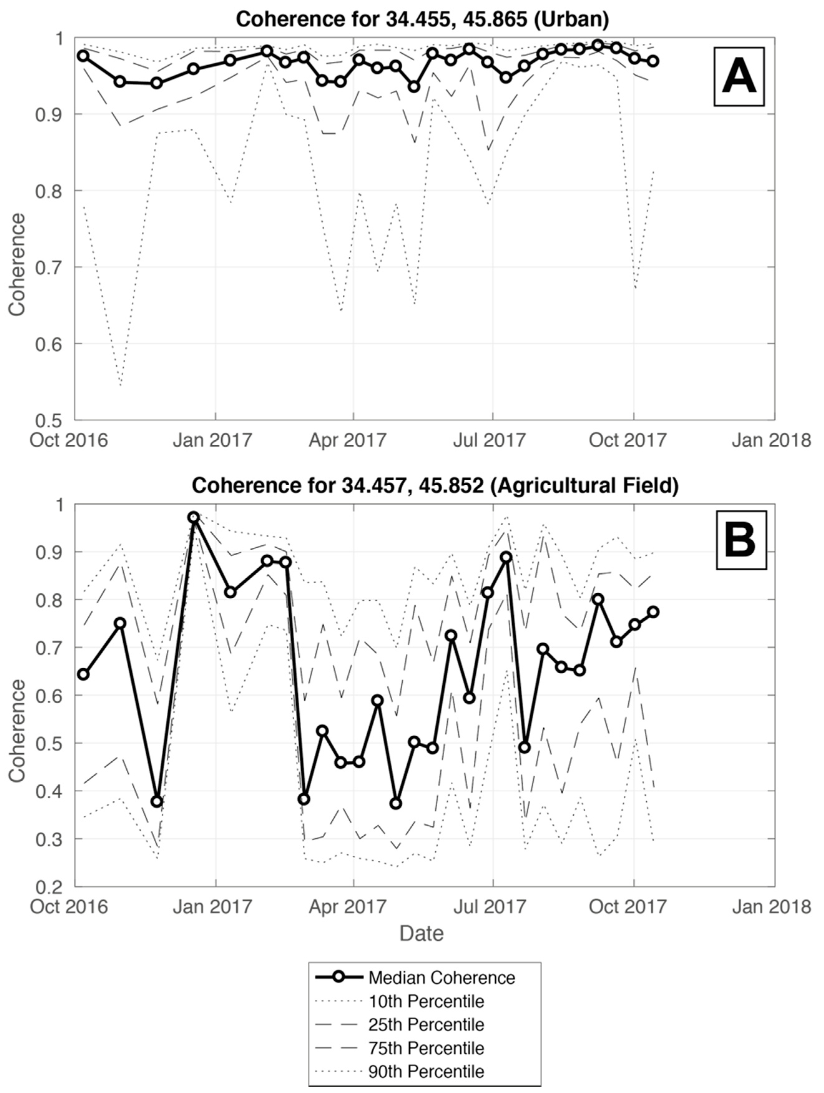
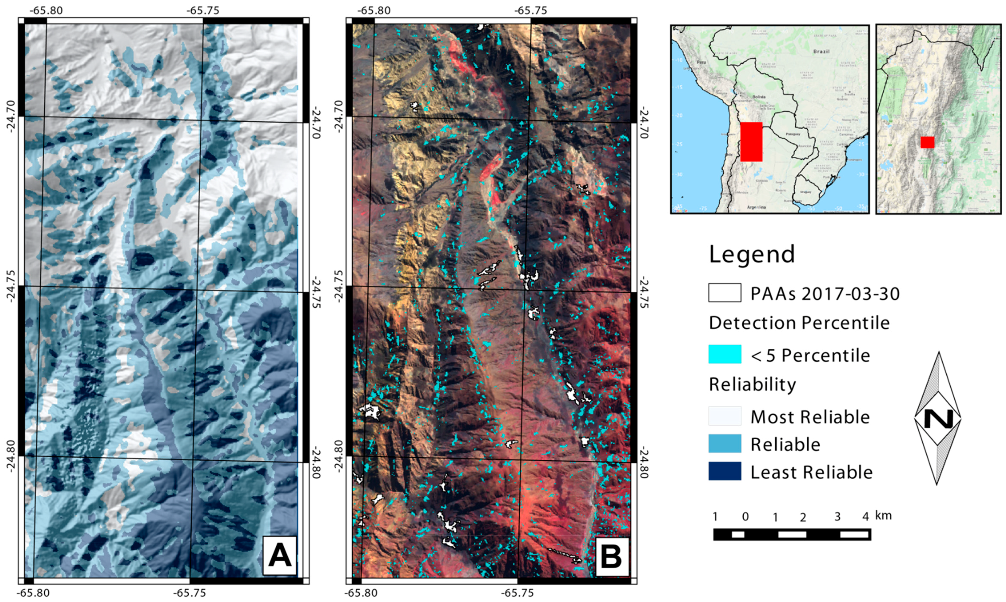
We generate a map of signal reliability derived from the standard deviation of coherence for each pixel to account for natural, non-event related coherence variability through time. In other words, a pixel that experiences considerable scatter throughout the course of a year, such as a forest or an agricultural field, will be considered less reliable when interpreting potentially affected areas than a pixel with little deviation through time, such as an urban structure. The reliability estimate is classified into three different categories: “least reliable”; “reliable”; and “most reliable”. For our case studies, we defined “most reliable” as having a standard deviation less than 0.1 (i.e., more than a ~68% of the time series varies less than a value of 0.1 as compared to a mean value), “reliable” as a standard deviation of 0.1–0.3, and “unreliable” as pixels with a standard deviation greater than 0.3. Reliability maps can also be optionally filtered to reduce noise and smooth patterns, though we did not perform this step in our case study analysis. Once produced, the reliability maps provide a basis for rapid interpretation of where coherence loss is most likely to be associated with damage from a natural hazard as opposed to natural variability.
The coherence for a single pixel is characterised over the time series in one of two ways: (1) using the entire data stack, including all times of year; or (2) using seasonally filtered stacks, depending on the timing of the event and the region of interest. If wet-dry seasonal cycles cause significant coherence variations in a time series, filtered coherence stacks, where only pre-event coherence from the wet or dry season is used, may be more appropriate for estimating PAAs (see Section 4.3 below). Ideally, the stack should not include dates containing known events of the type that the user wishes to detect. After the coherence stack is generated, potentially affected areas (PAAs) are identified by comparing syn-event coherence from a known or possible natural hazard event to the distribution of pre-event coherence values from the coherence data stack. To characterise where coherence values are abnormally low in the syn-event coherence image, each pixel of the syn-event image is compared to the temporal distribution (either annual or seasonal) of coherence values for that pixel and the inverse percentile of the syn-event coherence is calculated and assigned. The resulting map gives the percentile for each pixel compared to the distribution of past coherence values (e.g., 1st, 10th, 70th percentile). Regions that are below a user-defined critical threshold (e.g., 5th percentile) are considered potentially affected areas.
The inverse percentile map is binarised using a critical threshold value (e.g., 1st, 5th, 10th percentile) to determine PAAs. In regions with large areas of natural variability of coherence values (e.g., agricultural fields, forests), the reliability map can be used to filter the PAA estimation. The binary image is then amalgamated into connected components, providing a single numerical designation to each contiguous PAA region. Depending on the application, regions with few connected components can be filtered out. Using the map of PAA numerical identifications, PAAs can now be characterised in terms of user-specified properties, such as size, topography, population, and infrastructure statistics, and ranked accordingly. The method can also be used as a form of possible event detection and assessment in remote areas with minimal land-based monitoring infrastructure, by creating a background stack and reliability map, then feeding new SAR images as potential events to see if PAAs are detected.

3. Case Studies and Results

We implement our method in two independent case studies: (1) the 12 November 2017 Iran-Iraq earthquake near Sarpol-e, Iran, which caused significant damage to infrastructure and livelihood; and (2) the remote Quebrada del Toro in the Salta Province of Argentina in the south-central Andes, where we employ the method to detect possible, unrecorded events.

3.1. Case Study 1: 2017 Iran-Iraq Earthquake

On 12 November 2017, an oblique thrust-fault caused a 7.3 Mw earthquake at ~25 km depth on the border of Iran and Iraq that was one of the deadliest earthquakes of 2017. The earthquake caused significant damage to urban infrastructure, most of which was non-ductile concrete [23]. For our case study, we focus our region of interest around Sarpol-e Zahab, a city of ~45,000 inhabitants, located 50 km south-southwest of the earthquake epicentre, which was significantly damaged by the earthquake. We used approximately one year of Sentinel-1 data, including 28 SAR images from 7 October 2016 to 26 October 2016, to create the pre-event coherence stack (n = 27) for the Sarpol-e region of Iran (cf. Table 1, Supplemental Materials Table S1). The global Gridded Population of the World, v. 4 [24] is used to characterise population density (people per square kilometre) of the region. Figure 2A shows a Sentinel-2 false colour image of the Sarpol-e region, highlighting the extensive agriculture surrounding the urbanised region. Coherence values over the recorded time period are generally consistently high for urban structures (Figure 3A), but vary significantly in agricultural fields (Figure 3B). This is reflected in the reliability map, shown in Figure 2B, where agricultural areas are classified as “least reliable” due to the high natural variability of coherence.
Coherence was calculated for SAR images from 7 November and 19 November 2017. The syn-event coherence was then compared to the stack of 28 SAR scenes from the preceding year to calculate potentially affected areas. We identify 734 potentially affected areas with a total area of ~300 km2 in the event coherence image after we filter out the least reliable regions and PAAs with a contiguous area of less than 10 pixels (300 m2). Of the identified PAAs, 32% of them are in regions with population density higher than 50 people per square kilometre (cf. Table 2). PAA 4980 covers the region of Sarpol-e (Figure 2D), while PAA 7532 and 5318 overlap with other nearby settlements likely impacted by the earthquake. Sub-district estimates of population density, where available, will improve this ranking and easily differentiate PAAs that are highly populated (e.g., Sarpol-e; cf. Figure 2D) and those that are in a populated district, but do not overlap with developed areas (e.g., 4304; cf. Figure 2D). We rank PAAs by size and population density as an example that allows for easy prioritisation by decision makers and response teams; however, any user-defined criteria could be used to rank and filter the estimate of potentially affected areas.
Figure 4 highlights specific damage within the PAA (4980) covering Sarpol-e. Upon visual inspection using Google Earth historical imagery, several buildings within the PAA that were standing on 2 July 2017 (Figure 4A) have collapsed since the earthquake (Figure 4B). It is noteworthy that the individually damaged buildings fall within one PAA, due to the spatial resolution of the multilooked SAR coherence data. For example, if one building within a multilooked pixel has collapsed, and the neighbouring building within the same pixel has not, the entire pixel is marked as “potentially affected” and amalgamated with connected affected pixels into one contiguous PAA. Hence, a PAA may contain a mix of affected and unaffected pixels, making the identification of false positives difficult. To test the propensity for the method to create false positives, the PAA detection framework was additionally run for the dates directly preceding the 12 November earthquake, 26 October 2017 and 7 November 2017. During this quiescent time, we use the same PAA detection criteria as the time period covering the earthquake; however, no PAAs were detected in the Sarpol-e region. Hence, when there was not a corresponding natural hazard event triggering regional damage and surface change, no potentially false positives were detected by the PAA framework.

3.2. Case Study 2: Hillslope Activity and Landslide-Event Detection in the South-Central Andes

The Quebrada del Toro is an intermontane basin in the Salta district of northwestern Argentina, where several faults of the eastern margin of the Central Andes are tectonically active [28,29]. This valley provides the main transport route of mineral resources (REE, Lithium, Borate) from the central Andes (Puna de Atacama) to foreland factories and further processing. Remote communities and infrastructure in the Quebrada del Toro are vulnerable to sudden landslides, floods, and mudslides caused by at times isolated and remote rainfall events and seismically triggered hillslope instabilities [30,31,32,33]. As ground monitoring is limited in the Quebrada del Toro, it is an ideal location in which satellite monitoring may help identify such isolated events.
We employ approximately two years of Sentinel-1 data; 58 SAR scenes (mosaicked from 179 individual images to cover the entire region of interest) from 18 October 2014 to 30 December 2017 (cf. Table 1, Supplemental Materials Table S2). A series of SAR images from 2017 is used for potential event detection. The Global Precipitation Mission [26,27] data are used to evaluate precipitation in the Quebrada del Toro as a potential mass movement trigger.
We perform PAA identification for every image from the region for 2017 (5 January–7 December 2017) and compare the 2017 coherence values to the database of background coherence constructed from 18 October 2014 to 12 December 2016 to identify potential hazards that may impact communities or infrastructure. Because this region experiences a strongly seasonal precipitation regime, with a wet austral summer (November to April) and dry austral winter (May to October), we filter the coherence stacks by wet and dry seasons according to the first date of the syn-event coherence [30,31]. When detecting PAAs, we compared the pixel coherence to the background coherence from the filtered wet or dry stack. Figure 5 shows the results of the PAA detection for the interval between 18 March and 30 March 2017. This interval occurs during the wet season and following an interval of heightened precipitation (cf. Figure 6B). Here we focus on a steep-sided region of the valley hosting the main transit route between the Puna de Atacama and the city of Salta. Signal reliability decreases in the steepest sections of the valley (Figure 5A), but remains moderately to highly reliable along the valley floor where transport infrastructure is located.
After filtering for size (minimum 10 pixels or 300 m2) and reliability (discarding PAAs in “least reliable” classification), the algorithm detected eight possible PAAs that potentially intersect with transport lines along the valley floor (Figure 4B). No Google Earth historical imagery was available for March 2017 or later and both Landsat-8 and Sentinel-2 images from the time period are obscured by dense cloud cover; therefore, validation with visual inspection of satellite imagery was not possible. However, inspection of the detected PAAs intersecting with the main highway shows that the potentially affected regions are predominantly downslope of scree slopes and high-relief gullying (Figure 7), making them likely candidates for mudflows or landslides that are typical of the region.

4. Discussion

4.1. Advancements and Improvements Using Time Series of Coherence Data

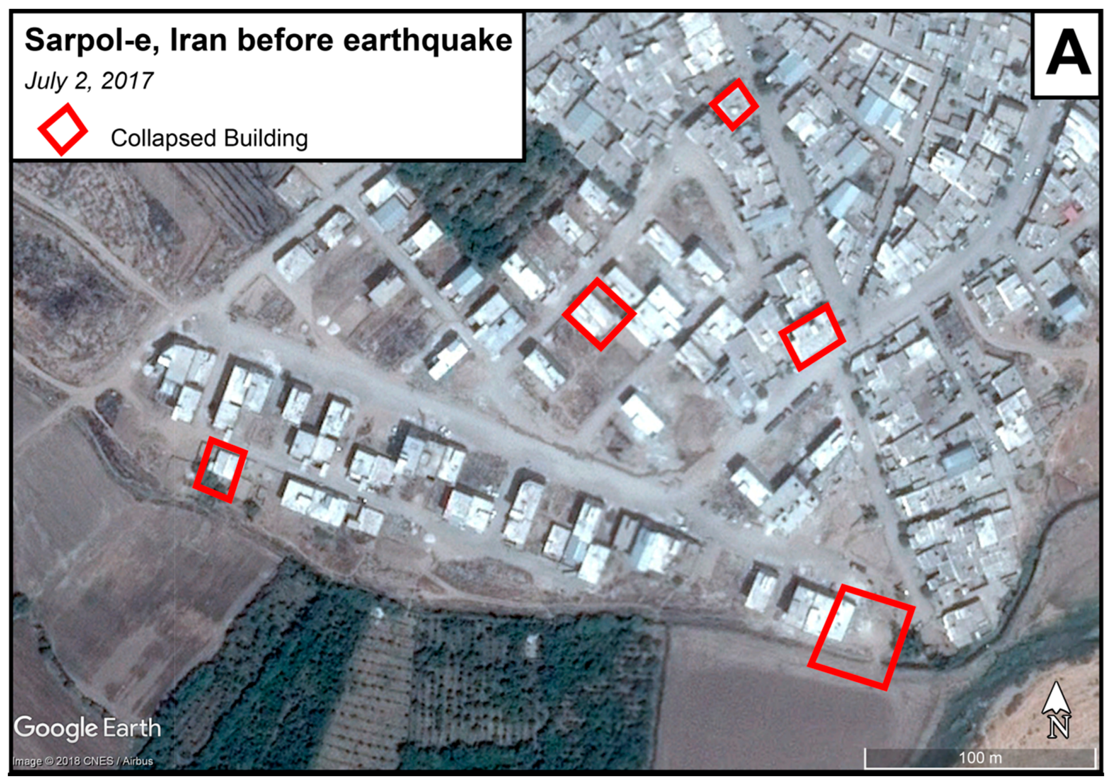
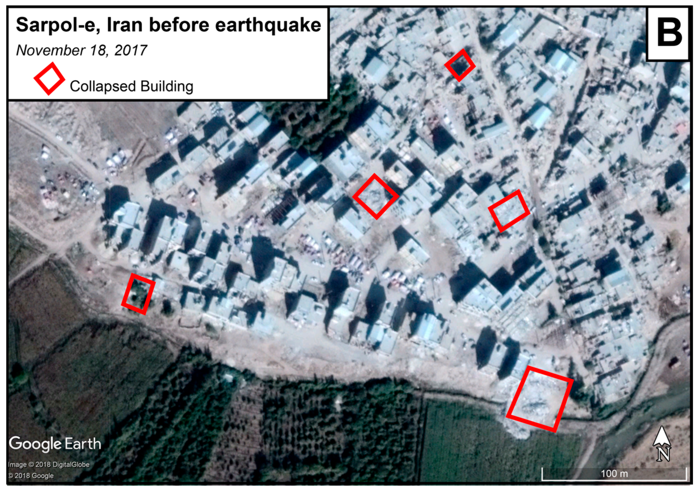
Weather- and daylight-independent, with near-global coverage and free accessibility, Sentinel-1 SAR data allows users to create robust databases of SAR values in regions of interest for natural hazard event detection and response. Using case studies from the region of Sarpol-e, Iran following the Mw 7.3 earthquake on 12 November 2017 and a major infrastructural hub for mineral resources in northwestern Argentina, we demonstrate how such databases can provide valuable insights into detecting potentially affected areas following natural hazard events.
The most important advancement of this method is the ability to create a pixel-by-pixel time series of coherence values over seasonal and meteorological cycles for a given region of interest. Variability of SAR coherence occurs due to natural cycles, such as wet-dry seasonal regional climatic patterns, but also due to anthropogenic causes, such as ploughing and growing seasons in agricultural areas. By constructing time series of each pixel’s coherence over these cycles, we determine where coherence loss is likely to be meaningful via the construction of reliability maps. These maps serve to guide user interpretation of detected PAAs. Constructing pixel-by-pixel time series of coherence allows the user to determine what magnitude of coherence loss is necessary for a given pixel in the region. For example, for a syn-event coherence value to fall below the, e.g., first percentile threshold for PAA detection, a lower coherence value will be required in regions with more inherent noise (e.g., a field or forest) than regions with less inherent noise (e.g., urban areas). This provides the user considerably more insight than a simple calculation of the coherence loss between syn-event coherence and a single pre-event coherence calculation. It also removes the need to alter the coherence data by means such as histogram matching to compare individual coherence estimates. The variability of coherence caused by atmospheric and other effects will be incorporated into the time series.
In regions where seasonal differences are important, the coherence stack can be filtered by season and the event compared directly to the range of coherence values in the appropriate season. Filtering the coherence values by season is particularly useful in regions with marked differences, e.g., rainy and dry seasons, or agricultural growing seasons. For example, meaningful coherence loss in the non-growing season may be encompassed by the inherent noisiness of the data if the growing season is included. To this end, a greater degree of coherence loss will be required during the growing season or the wet season than during times when coherence is more stable (e.g., dry season, outside of the growing season). This reduces the amount of noise during seasons with lower or more variable coherence, and ensures that event-related coherence loss during stable or high-coherence times is not missed because of a lower threshold when using the entire years’ coherence data. These subtler analyses of the syn-event coherence change are only possible by exploiting time series of pre-event coherence and cannot be gleaned from a single pre-event coherence estimate.
Multitemporal InSAR processing has been employed with high accuracy in other studies. For example, the use of persistent scatterers to track surface deformation and associated damage in urban environments, e.g., [34]. While a multitemporal InSAR approach using methods such as persistent scatterers provides insightful and accurate results, it requires that data collection and processing be performed after the event has occurred. This makes it poorly suited to rapid damage assessment. Pre-event coherence stacks and reliability maps in our proposed method can be calculated and maintained for a region of interest before a natural hazard event has occurred, meaning that the syn-event coherence is the only interferometric processing that needs to be performed after an event. Furthermore, coherence is a relatively simple calculation (compared to multitemporal interferometric processing with phase unwrapping or persistent scatterers analysis) that can be performed on a suite of different software platforms. Therefore, while our method does not provide the quantitative estimates of damage, it is a tool that can be rapidly generated following an event to aid user interpretation of potential damages.

4.2. Challenges of Mapping Potentially Affected Areas with Radar

Though the described processes offer a powerful and robust method to estimate regions potentially affected by natural hazard events, there are nonetheless inherent limitations to the method and the use of C-band radar. Most prominent of these is the applicability of C-band radar to highly vegetated regions. Because the wavelength of the C-band radar signal interacts with the vegetation canopy, e.g., [35,36], the coherence values of these regions may be too inherently noisy for meaningful assessment of affected areas using this method. To test the applicability of the method to densely vegetated regions, we used one year of SAR images of Freetown, Sierra Leone leading up to the large mudslides that devastated the densely populated city on 14 August 2017. No discernible patterns associated with the mudflow were detected in the event coherence image using this method. However, the launch of the Sentinel-1B satellite has increased the repeat time to 6–12 days, resulting in higher and more consistent coherence estimates between images with low temporal baseline (Figure 8). Thus, as more data are collected and the databases become increasingly robust to allow for better estimates of natural coherence variability, this problem may be constrained in the future.
In addition to vegetation, soil moisture or standing water directly impacts the coherence of two SAR images [37,38,39]. This may prove beneficial in the case of flood extent mapping [
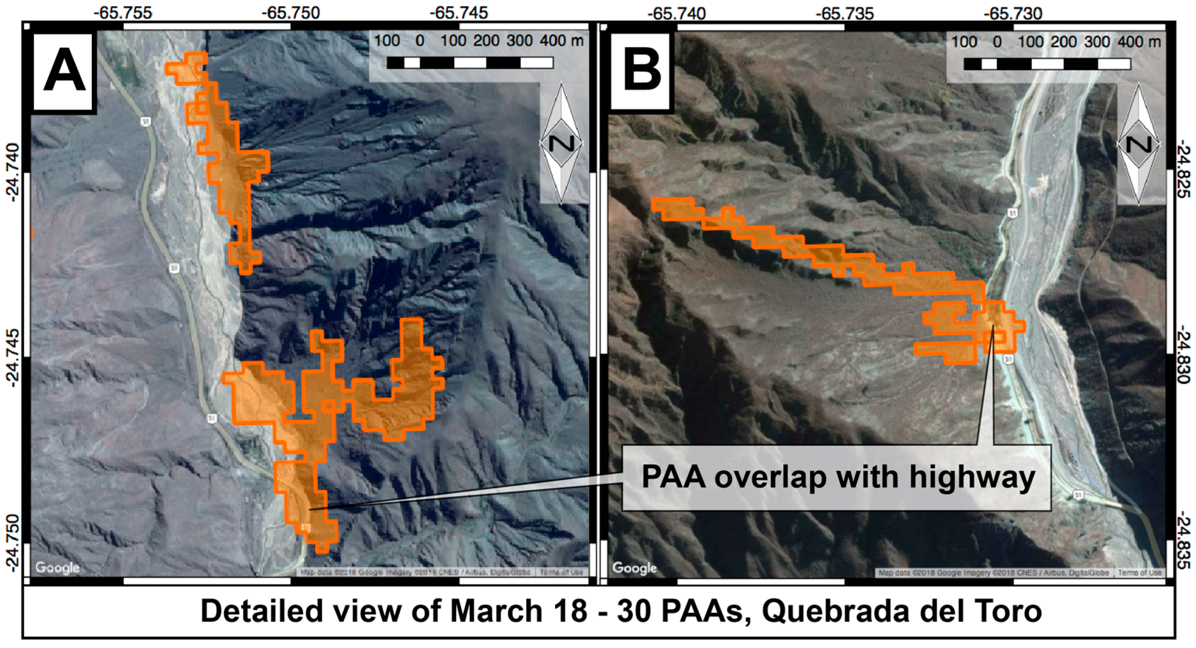
40], for example, but could result in extensive regions being flagged as potentially affected areas that have not experienced a triggering natural hazard event. This is of greater concern when the method is employed to detect potential events in remote regions, such as in our case study in the Quebrada del Toro. 
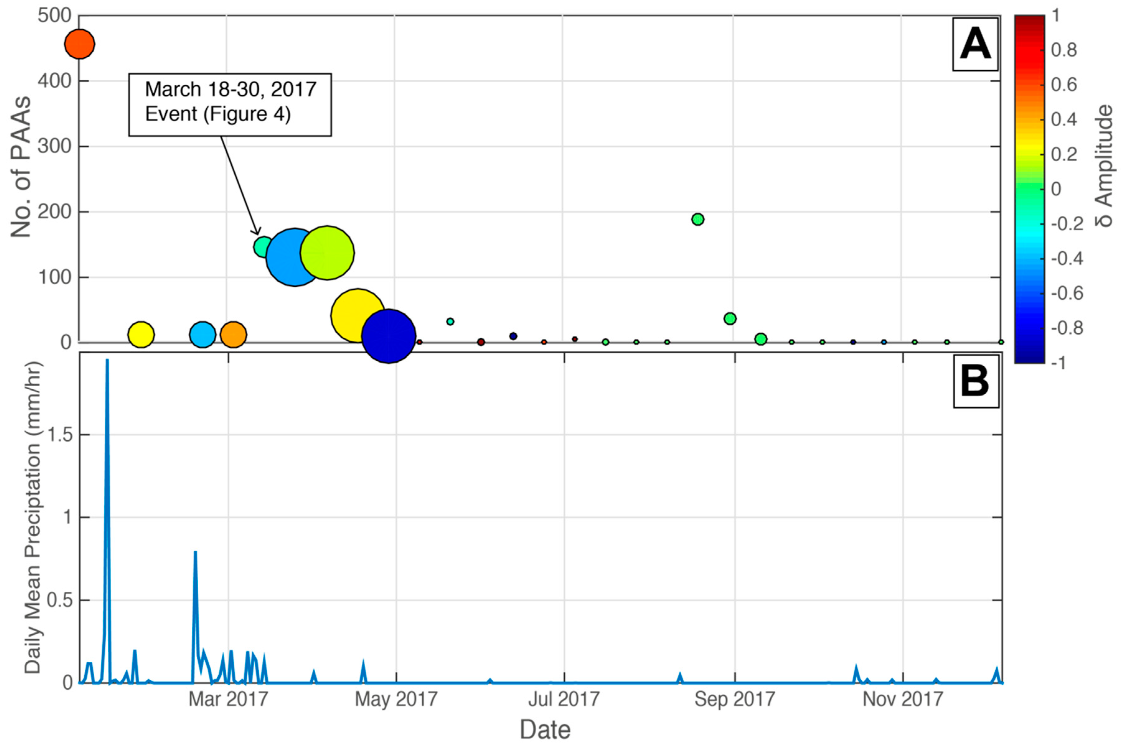
Figure 6 shows the number of PAAs detected in each coherence image and the size of the largest detected PAA compared to two indicators of potential soil moisture or standing water. The Global Precipitation Mission (GPM) precipitation records half-hour estimations of precipitation, but cannot always be directly linked to soil moisture. Therefore, we also use the change in Sentinel-1 amplitude (δAmplitude) between adjoining pairs as an additional proxy for soil moisture change. Though a limited number of independent soil moisture estimates exist (e.g., SMAP, CCI), they have proven unreliable in ground tests [41,42]. Because the presence of soil moisture, and particularly standing water, will result in a decrease in received radar amplitude, a negative change in amplitude (δAmplitude) between adjacent images may indicate an increase in soil moisture. Comparing these three time series, we observe that the largest and most extensive occurrences of PAAs in this region are associated with time intervals where changes soil moisture are likely to be impacting large areas of the scene. We observe order-of-magnitude larger contiguous PAA area in time intervals with negative δAmplitude compared to, e.g., during the March 2017 example highlighted in Section 3.2. While this does not provide a quantitative estimate of soil moisture, incorporating additional data constraints, such as GPM and soil moisture proxies, can aid in the interpretation of large and extensive PAAs to determine if a detected event is likely to be hazardous or resulting from soil moisture change.

4.3. Length and Temporal Spacing of Coherence Database

There are two main considerations when determining how large the database of coherence values should be for a given region of interest. Though larger databases will result in more robust estimates, due to storage and computing capacity issues, users may want to use the minimum database size reasonable. Therefore, users should consider: (1) how coherent a region is likely to be; and (2) are there important seasonal cycles in the region of interest? For example, in the case study in Sarpol-e, Iran, we expect generally high coherence values due to the arid nature of the region. A temperate region will require a longer time series to get accurate estimates of coherence variability. However, even in regions that are semi-arid, seasonal cycles may cause large variation in coherence values between dry and wet seasons. If the region requires separate seasonal coherence databases, a longer time series will be desirable to ensure that each seasonal database remains robust.
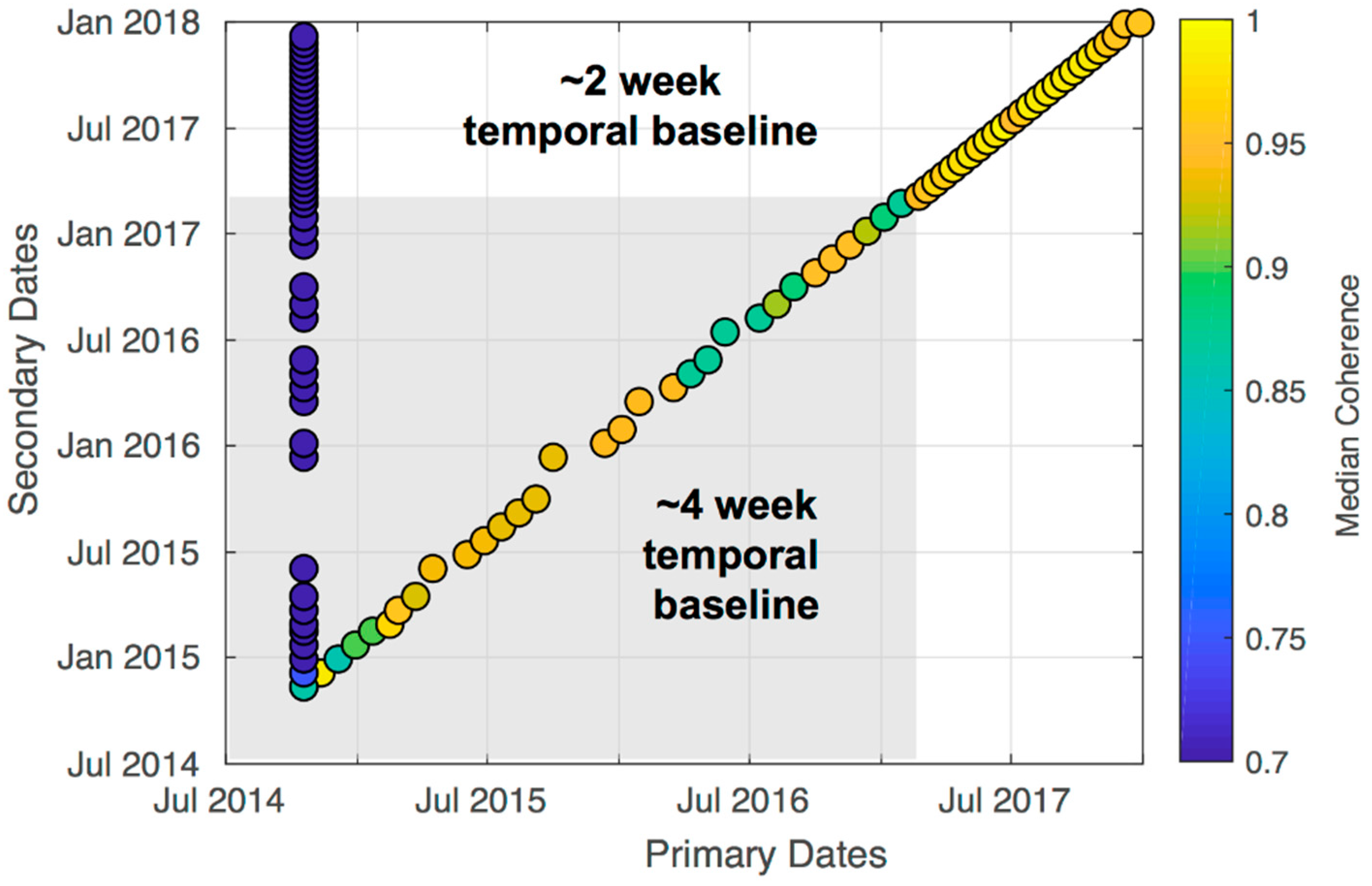
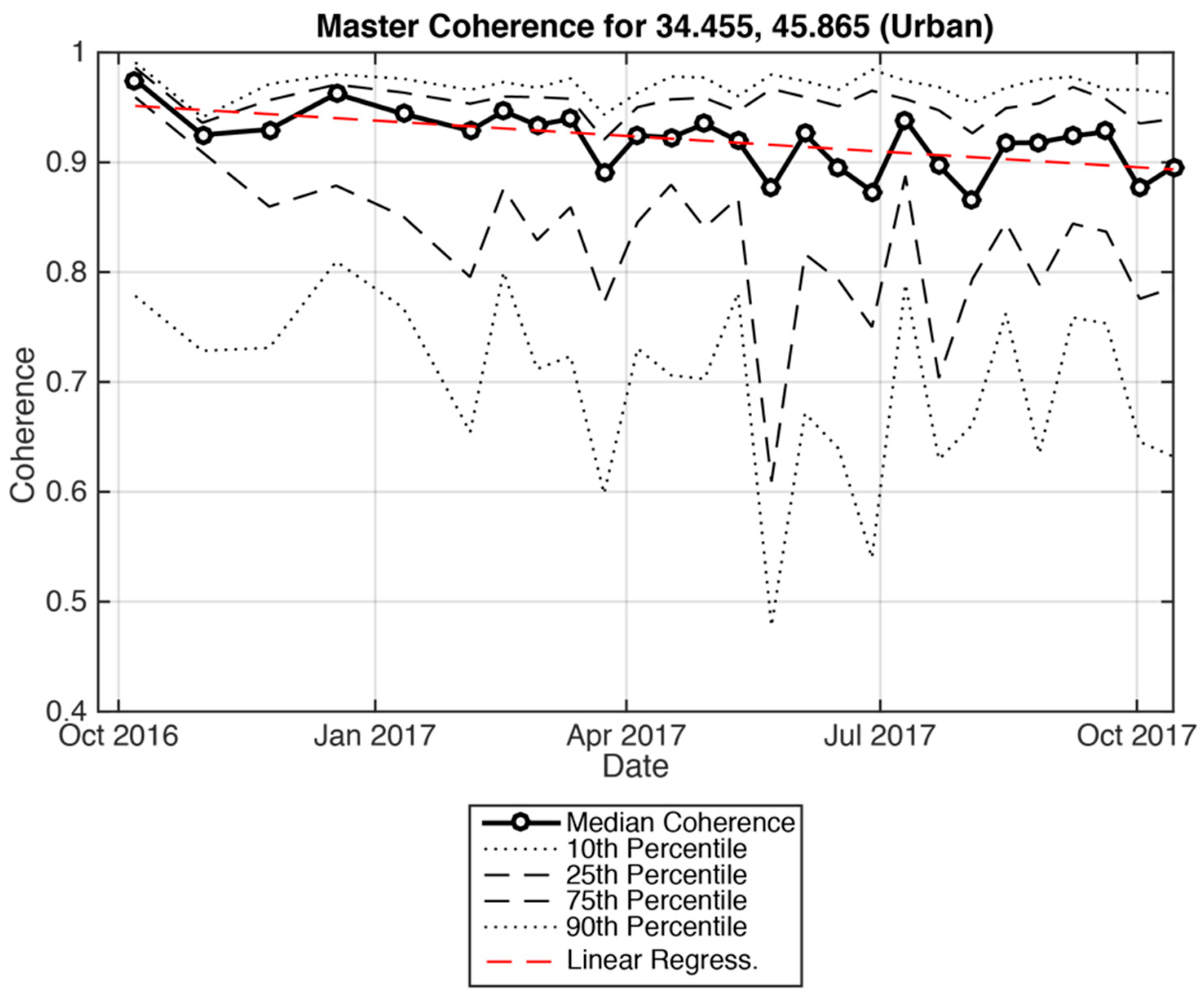
Another consideration is the temporal spacing of SAR scenes in the database. After the launch of Sentinel-1B (April 2016), the recurrence interval of SAR data collection of a region has regularised. However, users who desire longer time series may encounter the problem that the recurrence interval was longer during the period where only Sentinel-1A is available. A natural deterioration of coherence occurs with increasing temporal baseline between SAR images, even for regions that are coherent. Figure 9 shows the decrease in coherence for a coherent urban region of Sarpol-e, Iran. Though a gradual decrease in coherence (~0.0014/week, R = −0.608) is observed with time, approximately six months are required before the coherence drops below 0.9. We therefore infer that the inherent coherence loss between two- and four-week temporal baselines should be minimal. In the case that the inherent decrease in coherence is high, a simple normalisation of values in the pre-event coherence stack by temporal baseline can be implemented. However, when possible, it is always desirable to use as consistent of temporal baseline as possible.

5. Conclusions

The open accessibility, near-global coverage, and high repeat time of Sentinel-1 C-band radar allows for new advances in monitoring natural hazards on the Earth’s surface. By constructing a database of SAR coherence values for regions of interest, where seismic or climatically triggered natural hazards are likely to occur, we can now determine where coherence loss is meaningful, and what magnitude of coherence loss related to an event is necessary to determine potentially affected areas. Though the construction of a large coherence database may be computationally expensive and time-consuming, this step can be done pre-emptively for regions of interest and maintained as new data becomes available. The temporal database of coherence values can then be rapidly employed to estimate damage following a natural hazard event. By using a time series of coherence values to characterise the pre-event coherence, we account for the natural variability of coherence inherent to different land covers across a region of interest. Furthermore, the method can be used not only for rapid response following known events (e.g., earthquakes, heavy precipitation), but as a detection tool in remote regions where events may go undetected by traditional monitoring means. Though we focus our study on C-band radar provided by ESA’s Sentinel-1 mission, due to its high accessibility, we point out that it could also improve potential damage mapping using other radar bands provided a long enough time series is acquired. This is particularly true for X-band radar systems such as COSMO-SkyMed or TerraSAR-X, where different acquisition modes have a much higher spatial resolution, but are also highly sensitive to surficial changes.
The estimation of potentially affected areas following this method, combined with pertinent local data (e.g., population, infrastructure) creates a valuable tool for identifying and interpreting regions that may be damaged following a natural hazard event. By understanding, quantifying, and mapping the natural variability of coherence in a region of interest, both scientists and response teams will be able to more effectively respond to the growing number of natural hazards posed by our increasingly changing and volatile global system.

Supplementary Materials

The following are available online at https://www.mdpi.com/2072-4292/10/8/1272/s1. Table S1: Sentinel-1 data used for the Iran database and event analysis, Table S2: Sentinel-1 data used for the Quebrada del Toro database and event detection.

Author Contributions

Conceptualisation, S.O. and B.B.; Methodology, S.O. and B.B.; Validation, S.O. and B.B.; Writing-Original Draft Preparation, S.O.; Writing-Review & Editing, S.O. and B.B.; Visualisation, S.O. and B.B.; Funding Acquisition, B.B.

Funding

This research was funded by German Research Foundation (Deutsche Forschungsgemeinschaft) grant number DFG BO 2933/3-1 and DLR project DIGENTI (50RP1502).

Acknowledgments

We thank Jordi Tost of the Interactive Design Lab, Fachhochschule Potsdam for insightful discussion; and three anonymous reviewers for their constructive feedback on this work. We acknowledge the support of the German Research Foundation and Open Access Publishing Fund of University of Potsdam.

Conflicts of Interest

The authors declare no conflict of interest.

References

  1. Joyce, K.E.; Belliss, S.E.; Samsonov, S.V.; McNeill, S.J.; Glassey, P.J. A review of the status of satellite remote sensing and image processing techniques for mapping natural hazards and disasters. Prog. Phys. Geogr. 2009, 33, 183–207. [Google Scholar] [CrossRef]
  2. Tralli, D.M.; Blom, R.G.; Zlotnicki, V.; Donnellan, A.; Evans, D.L. Satellite remote sensing of earthquake, volcano, flood, landslide and coastal inundation hazards. ISPRS J. Photogramm. Remote Sens. 2005, 59, 185–198. [Google Scholar] [CrossRef]
  3. Kääb, A. Remote sensing of permafrost-related problems and hazards. Permafr. Periglac. Process. 2008, 19, 107–136. [Google Scholar] [CrossRef]
  4. Bürgmann, R.; Rosen, P.A.; Fielding, E.J. Synthetic aperture radar interferometry to measure Earth’s surface topography and its deformation. Annu. Rev. Earth Planet. Sci. 2000, 28, 169–209. [Google Scholar] [CrossRef]
  5. Touzi, R.; Lopes, A.; Bruniquel, J.; Vachon, P.W. Coherence estimation for SAR imagery. IEEE Trans. Geosci. Remote Sens. 1999, 37, 135–149. [Google Scholar] [CrossRef]
  6. Yun, S.-H.; Hudnut, K.; Owen, S.; Webb, F.; Simons, M.; Sacco, P.; Gurrola, E.; Manipon, G.; Liang, C.; Fielding, E.; et al. Rapid Damage Mapping for the 2015 M w 7.8 Gorkha Earthquake Using Synthetic Aperture Radar Data from COSMO--SkyMed and ALOS-2 Satellites. Seismol. Res. Lett. 2015, 86, 1549–1556. [Google Scholar] [CrossRef]
  7. Fielding, E.J.; Talebian, M.; Rosen, P.A.; Nazari, H.; Jackson, J.A.; Ghorashi, M.; Walker, R. Surface ruptures and building damage of the 2003 Bam, Iran, earthquake mapped by satellite synthetic aperture radar interferometric correlation. J. Geophys. Res. Solid Earth 2005, 110. [Google Scholar] [CrossRef] [Green Version]
  8. Hoffmann, J. Mapping damage during the Bam (Iran) earthquake using interferometric coherence. Int. J. Remote Sens. 2007, 28, 1199–1216. [Google Scholar] [CrossRef]
  9. Yonezawa, C.; Takeuchi, S. Decorrelation of SAR data by urban damages caused by the 1995 Hyogoken-nanbu earthquake. Int. J. Remote Sens. 2001, 22, 1585–1600. [Google Scholar] [CrossRef]
  10. Watanabe, M.; Motohka, T.; Miyagi, Y.; Yonezawa, C.; Shimada, M. Analysis of Urban Areas Affected by the 2011 Off the Pacific Coast of Tohoku Earthquake and Tsunami With L-Band SAR Full-Polarimetric Mode. IEEE Geosci. Remote Sens. Lett. 2012, 9, 472–476. [Google Scholar] [CrossRef]
  11. Sharma, C.R.; Tateishi, R.; Hara, K.; Nguyen, T.H.; Gharechelou, S.; Nguyen, V.L. Earthquake Damage Visualization (EDV) Technique for the Rapid Detection of Earthquake-Induced Damages Using SAR Data. Sensors 2017, 17, 235. [Google Scholar] [CrossRef] [PubMed]
  12. Werninghaus, R.; Buckreuss, S. The TerraSAR-X mission and system design. IEEE Trans. Geosci. Remote Sens. 2010, 48, 606–614. [Google Scholar] [CrossRef] [Green Version]
  13. Covello, F.; Battazza, F.; Coletta, A.; Lopinto, E.; Fiorentino, C.; Pietranera, L.; Valentini, G.; Zoffoli, S. COSMO-SkyMed an existing opportunity for observing the Earth. J. Geodyn. 2010, 49, 171–180. [Google Scholar] [CrossRef] [Green Version]
  14. Torres, R.; Snoeij, P.; Geudtner, D.; Bibby, D.; Davidson, M.; Attema, E.; Potin, P.; Rommen, B.; Floury, N.; Brown, M.; et al. GMES Sentinel-1 mission. Remote Sens. Environ. 2012, 120, 9–24. [Google Scholar] [CrossRef]
  15. Geudtner, D.; Torres, R.; Snoeij, P.; Davidson, M.; Rommen, B. Sentinel-1 system capabilities and applications. In Proceedings of the 2014 IEEE International Geoscience and Remote Sensing Symposium (IGARSS), Quebec, QC, Canada, 13–18 July 2014; pp. 1457–1460. [Google Scholar]
  16. Moreira, A.; Prats-Iraola, P.; Younis, M.; Krieger, G.; Hajnsek, I.; Papathanassiou, K.P. A tutorial on synthetic aperture radar. IEEE Geosci. Remote Sens. Mag. 2013, 1, 6–43. [Google Scholar] [CrossRef] [Green Version]
  17. Zebker, H.A.; Villasenor, J. Decorrelation in interferometric radar echoes. IEEE Trans. Geosci. Remote Sens. 1992, 30, 950–959. [Google Scholar] [CrossRef] [Green Version]
  18. InSAR Scientific Computing Environment—The Home Stretch. Available online: https://trs.jpl.nasa.gov/bitstream/handle/2014/43527/11-5426_A1b.pdf?sequence=1&isAllowed=y (accessed on 13 August 2018).
  19. InSAR Scientific Computing Environment. Available online: http://abstractsearch.agu.org/meetings/2010/FM/IN43B-1397.html (accessed on 13 August 2018).
  20. Agram, P.S.; Jolivet, R.; Riel, B.; Lin, Y.N.; Simons, M.; Hetland, E.; Doin, M.-P.; Lasserre, C. New radar interferometric time series analysis toolbox released. Eos Trans. Am. Geophys. Union 2013, 94, 69–70. [Google Scholar] [CrossRef]
  21. Farr, T.G.; Rosen, P.A.; Caro, E.; Crippen, R.; Duren, R.; Hensley, S.; Kobrick, M.; Paller, M.; Rodriguez, E.; Roth, L. The shuttle radar topography mission. Rev. Geophys. 2007, 45. [Google Scholar] [CrossRef]
  22. Copernicus Open Access Hub. Available online: https://scihub.copernicus.eu/ (accessed on 13 August 2018).
  23. United States Geological Survey (USGS). M 7.3–29 km S of Halabjah, Iraq; USGS: Reston, VA, USA, 2017.
  24. Gridded Population of the World, Version 4 (GPWv4), Revision; Models the Distribution of Human Population (Counts and Densities) on a Continuous Global Raster Surface; Center for International Earth Science Information Network (EOSDIS): Palisades, NY, USA, 2017.
  25. Google Earth Engine. Available online: https://code.earthengine.google.com/ (accessed on 13 August 2018).
  26. Hou, A.Y.; Kakar, R.K.; Neeck, S.; Azarbarzin, A.A.; Kummerow, C.D.; Kojima, M.; Oki, R.; Nakamura, K.; Iguchi, T. The Global Precipitation Measurement Mission. Bull. Am. Meteorol. Soc. 2014, 95, 701–722. [Google Scholar] [CrossRef] [Green Version]
  27. Smith, E.A.; Asrar, G.; Furuhama, Y.; Ginati, A.; Mugnai, A.; Nakamura, K.; Adler, R.F.; Chou, M.-D.; Desbois, M.; Durning, J.F.; et al. International global precipitation measurement (GPM) program and mission: An overview. In Measuring Precipitation from Space; Springer: Berlin, Germany, 2007; pp. 611–653. [Google Scholar]
  28. Hilley, G.E.; Strecker, M.R. Processes of oscillatory basin filling and excavation in a tectonically active orogen: Quebrada del Toro Basin, NW Argentina. Geol. Soc. Am. Bull. 2005, 117, 887–901. [Google Scholar] [CrossRef]
  29. Tofelde, S.; Schildgen, T.F.; Savi, S.; Pingel, H.; Wickert, A.D.; Bookhagen, B.; Wittmann, H.; Alonso, R.N.; Cottle, J.; Strecker, M.R. 100 kyr fluvial cut-and-fill terrace cycles since the Middle Pleistocene in the southern Central Andes, NW Argentina. Earth Planet. Sci. Lett. 2017, 473, 141–153. [Google Scholar] [CrossRef]
  30. Bookhagen, B.; Strecker, M.R. Orographic barriers, high-resolution TRMM rainfall, and relief variations along the eastern Andes. Geophys. Res. Lett. 2008, 35. [Google Scholar] [CrossRef] [Green Version]
  31. Castino, F.; Bookhagen, B.; Strecker, M.R. River-discharge dynamics in the Southern Central Andes and the 1976–77 global climate shift. Geophys. Res. Lett. 2016, 43, 11679–11687. [Google Scholar] [CrossRef]
  32. Castino, F.; Bookhagen, B.; Strecker, M.R. Rainfall variability and trends of the past six decades (1950–2014) in the subtropical NW Argentine Andes. Clim. Dyn. 2017, 48, 1049–1067. [Google Scholar] [CrossRef]
  33. Purinton, B.; Bookhagen, B. Measuring Decadal Vertical Land-level Changes from SRTM-C (2000) and TanDEM-X (~2015) in the South-Central Andes. Earth Surf. Dyn. 2018. [Google Scholar] [CrossRef]
  34. Milillo, P.; Giardina, G.; DeJong, J.M.; Perissin, D.; Milillo, G. Multi-Temporal InSAR Structural Damage Assessment: The London Crossrail Case Study. Remote Sens. 2018, 10, 287. [Google Scholar] [CrossRef]
  35. Askne, J.I.H.; Dammert, P.B.G.; Ulander, L.M.H.; Smith, G. C-band repeat-pass interferometric SAR observations of the forest. IEEE Trans. Geosci. Remote Sens. 1997, 35, 25–35. [Google Scholar] [CrossRef]
  36. Hagberg, J.O.; Ulander, L.M.H.; Askne, J. Repeat-pass SAR interferometry over forested terrain. IEEE Trans. Geosci. Remote Sens. 1995, 33, 331–340. [Google Scholar] [CrossRef]
  37. Ulaby, F.T.; Dubois, P.C.; Van Zyl, J. Radar mapping of surface soil moisture. J. Hydrol. 1996, 184, 57–84. [Google Scholar] [CrossRef]
  38. Moran, M.S.; Hymer, D.C.; Qi, J.; Sano, E.E. Soil moisture evaluation using multi-temporal synthetic aperture radar (SAR) in semiarid rangeland. Agric. For. Meteorol. 2000, 105, 69–80. [Google Scholar] [CrossRef] [Green Version]
  39. Scott, C.P.; Lohman, R.B.; Jordan, T.E. InSAR constraints on soil moisture evolution after the March 2015 extreme precipitation event in Chile. Sci. Rep. 2017, 7, 4903. [Google Scholar] [CrossRef] [PubMed]
  40. Martinis, S.; Twele, A.; Voigt, S. Towards operational near real-time flood detection using a split-based automatic thresholding procedure on high resolution TerraSAR-X data. Nat. Hazards Earth Syst. Sci. 2009, 9, 303–314. [Google Scholar] [CrossRef] [Green Version]
  41. Ray, R.L.; Fares, A.; He, Y.; Temimi, M. Evaluation and Inter-Comparison of Satellite Soil Moisture Products Using In Situ Observations over Texas, US. Water 2017, 9, 372. [Google Scholar] [CrossRef]
  42. Dorigo, W.; Scipal, K.; Parinussa, R.M.; Liu, Y.Y.; Wagner, W.; De Jeu, R.A.M.; Naeimi, V. Error characterisation of global active and passive microwave soil moisture data sets. Hydrol. Earth Syst. Sci. 2010, 7, 5621–5645. [Google Scholar] [CrossRef]
Figure 1. Diagram illustrating the workflow of the potentially affected area (PAA) detection. Data input is denoted by blue parallelograms; processes are shown as white rectangles, algorithm-generated geotiffs are shown as yellow documents; and the output PAA locations and statistics are shown in the red terminal rectangle. The generation of the coherence database and the reliability map can be completed before an event has occurred (left hand of flow chart). After an event has occurred, the pre- and post-event SAR images can be input into the algorithm, as well as any pertinent additional information (e.g., population count, infrastructure, resources), to detect and characterise PAAs.
Remotesensing 10 01272 g001
Figure 2. Results of the PAA-detection algorithm following the 12 November 2017 earthquake near Sarpol-e, Iran. (A) False-colour Sentinel-2 composite (R = Near Infrared, G = Red, B = Green) of the region, highlighting the presence of agricultural fields outside of the city of Sarpol-e (shown in red in the false colour composite). Location of coherence time series shown in Figure 3A is denoted by a yellow triangle and Figure 3B. by a white triangle; (B) Reliability map of the Sarpol-e region, based on the variability of coherence data in the year preceding the earthquake. Note that the vegetated agricultural fields visible in (A) are classified as “least reliable” due to the high noise associated with vegetated surfaces using C-band radar; (C) All regions (shown in blue) where the coherence of the pre- and post-event pair were less than the 5th percentile of the annual coherence distribution, before connected components and filtering are performed; (D) The five largest, most populous PAAs detected in relation to the 12 November 2017 earthquake (cf. Table 2). Inset map data: Google Maps.
Remotesensing 10 01272 g002
Figure 3. Time series of coherence preceding the 12 November 2017 earthquake for (A) An urban structure (yellow triangle in Figure 2A); and (B) Agricultural field (white inverted triangle in Figure 2A) in the region of Sarpol-e, Iran. Coherence was calculated for each adjacent date (e.g., date-1 & date-2; date-2 & date-3) and averaged over a 10 × 10 pixel window. This highlights the differences between coherence over time in regions classified as “most reliable” (A) and “least reliable” (B).
Remotesensing 10 01272 g003
Figure 4. Detail of damage to buildings in Sarpol-e, Iran using Google Earth historical imagery. Collapsed buildings are highlighted in red. All damage is within PAA 4980 covering the city of Sarpol-e. The PAA detection using Sentinel-1 imagery does not identify damage to specific buildings, but detects areas containing damage.
Remotesensing 10 01272 g004aRemotesensing 10 01272 g004b
Figure 5. Example of the potentially affected area algorithm in use for event detection in the Quebrada del Toro, Argentina. (A) Reliability map for region. This highlights that in very steep areas, such as the highlighted section of the valley, coherence values are noisier and more complicated to interpret; (B) False-colour Sentinel-2 composite the region of interest with the results of the PAA algorithm for the period between 18 March and 30 March 2017, following a period of intensified rainfall (cf. Figure 6). All regions below the 5th percentile of coherence values 2014–2016 are shown in blue. PAAs (<1st percentile) are shown in white. PAAs detected in steep sections of the valley such as this may pose a threat to critical transport infrastructure between the Puna de Atacama plateau and the Andean foreland. Inset map data: Google Maps.
Remotesensing 10 01272 g005
Figure 6. Comparison of the number of potentially affected areas detected in the Quebrada del Toro (A) to regional rainfall as recorded by the Global Precipitation Mission (B). (A) The number of PAAs detected per time interval, with symbol sizes scaled linearly to the largest contiguous PAA for a given date (dates with no PAAs detected were given an arbitrarily small symbol size). We hypothesise that large contiguous PAAs are likely the result of soil moisture changes rather than potential land surface movements (e.g., debris flows, mudflows). The change in amplitude between scenes is used as a proxy for changes in soil moisture, where negative δAmplitude suggests increased soil moisture. Dates with smaller maximum PAA area and δAmplitude ≈ 0 are more likely to contain PAAs unrelated to soil moisture change.
Remotesensing 10 01272 g006
Figure 7. Details of PAA overlap with highway infrastructure. Satellite optical images from this time are obscured by cloud cover, but detected PAAs are located downslope of scree slopes and gullying (A) and high-relief surfaces (B) with potential for landslides or mudflows. Satellite imagery from Google Earth Pro, CNES/Airbus, and Digital Globe.
Remotesensing 10 01272 g007
Figure 8. Coherence values averaged over the entire region of interest for all date combinations used in the Quebrada del Toro case study. Though interferometric coherence in images where the temporal spacing is larger, coherence values since the launch of Sentinel1-B have been generally high and will, going forward, result in more robust time series than presently available.
Remotesensing 10 01272 g008
Figure 9. Coherence loss with a decrease of ~0.0014/week (R = −0.608) from a primary date (7 October 2016) to all subsequent secondary dates for a stable, coherent region (urban building) in Sarpol-e, Iran (see Figure 2A for location), demonstrating the protracted decrease in interferometric coherence with time. Because the low rate of decay of the coherence signal in stable areas, we deem it acceptable to compare the ~4-week recurrence interval Sentinel-1A SAR images to the ~2-week recurrence interval Sentinel-1A/B images.
Remotesensing 10 01272 g009
Table 1. Summary of data used in case studies, date ranges, application, and sources.
DatasetDatesApplicationTrack, OrientationSourceWebsite
Sentinel-1 Iran: 28 SAR images7 October 2016 through 19 November 2017Coherence MeasurementsDescending, Track 6ESA [22]https://scihub.copernicus.eu/
Sentinel-1 Argentina: 58 SAR images18 October 2014 through 30 December 2017Coherence MeasurementsDescending, Track 10ESA [22]https://scihub.copernicus.eu/
Sentinel-22017 minimum value compositeFalse colour composite ESA/Google Earth Engine [25]https://code.earthengine.google.com/
SRTM-C 1 arc second global DEMFebruary 2000SAR topographic correction NASA/USGS [21]https://lta.cr.usgs.gov/SRTM1Arc
Gridded Population of the World, Version 4 (GPWv4)2015Risk analysis Center for International Earth Science Information Network—CIESIN [24] http://sedac.ciesin.columbia.edu/data/collection/gpw-v4
Global Precipitation Mission5 January 2017 through 7 December 2017Risk analysis JAXA/NASA [26,27] https://www.nasa.gov/mission_pages/GPM/main/index.html
Table 2. Iran-Iraq Mw 7.3 PAA statistics for five most populous and largest detected PAAs (cf. Figure 2D).
PAA IDLocation (Lat, Lon) (Decimal Degrees)Area (km2)Population Density (people/km2)Average CoherenceMinimum CoherenceMunicipalities
498034.4120, 45.86356.580896.750.4950.195Sarpol-e
753234.3061, 45.99765.085996.750.4390.192Abuzar Garrison
531834.4137, 45.87021.109796.750.6710.201Gheitek, Moshkenar
801434.2908, 46.01570.873996.750.6580.235Neghare Kub
430434.4576, 45.81810.820896.740.4810.206NA

