Remote Sensing Derived Built-Up Area and Population Density to Quantify Global Exposure to Five Natural Hazards over Time

 , , , , , and
Abstract

1. Introduction
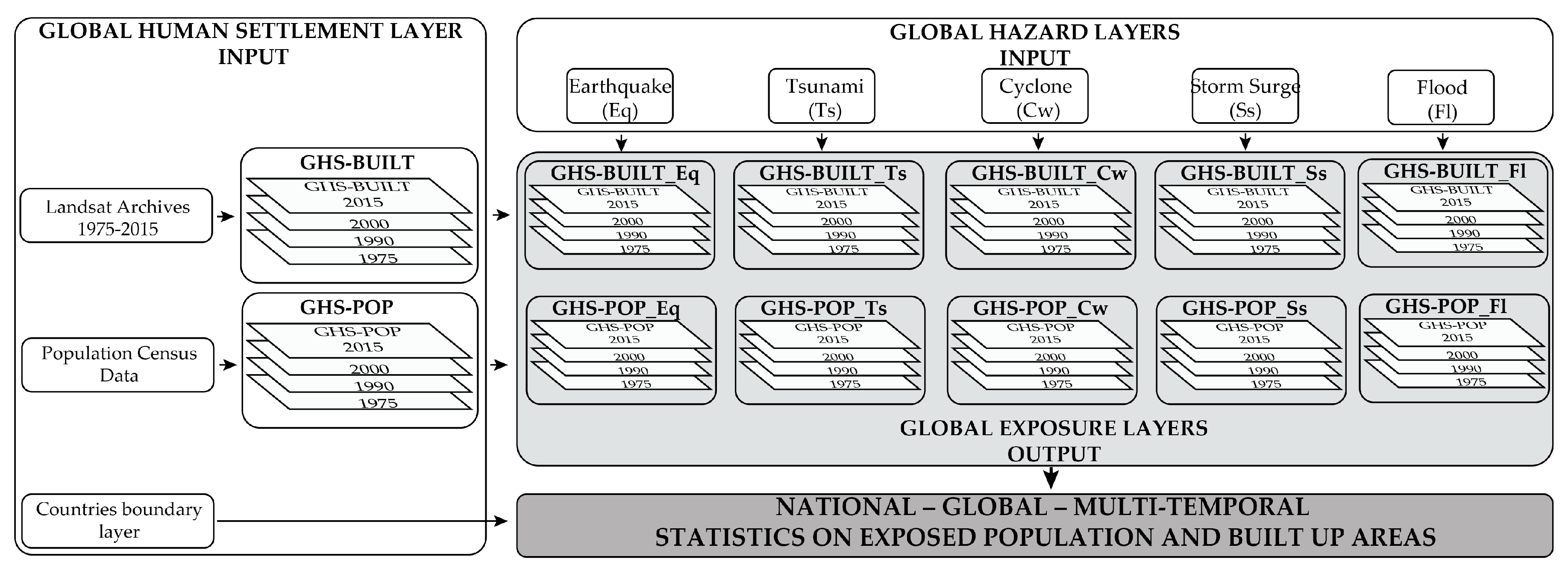
2. Data and Methods
2.1. Input Data
2.1.1. Global Built-Up Area
2.1.2. Global Population Density
2.1.3. Hazard Maps
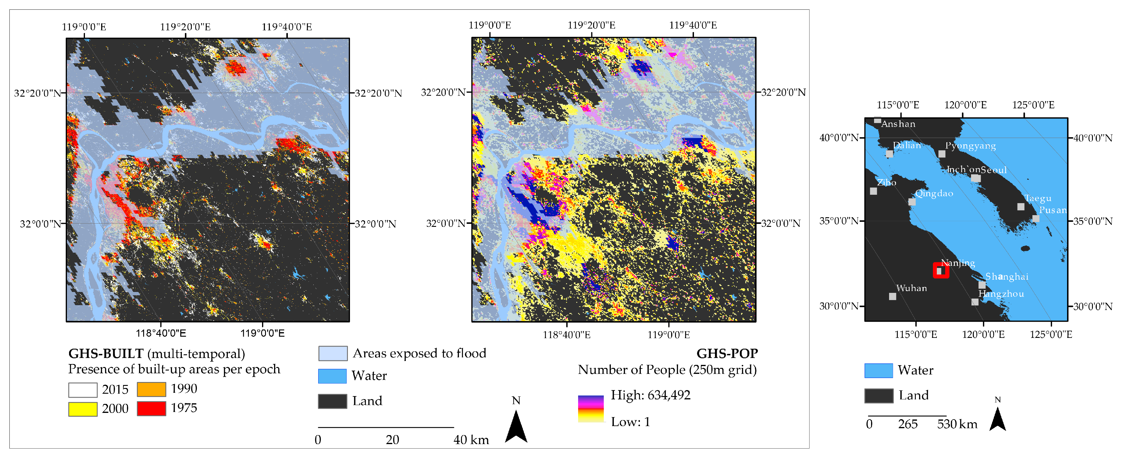
2.2. Methodology
3. Results
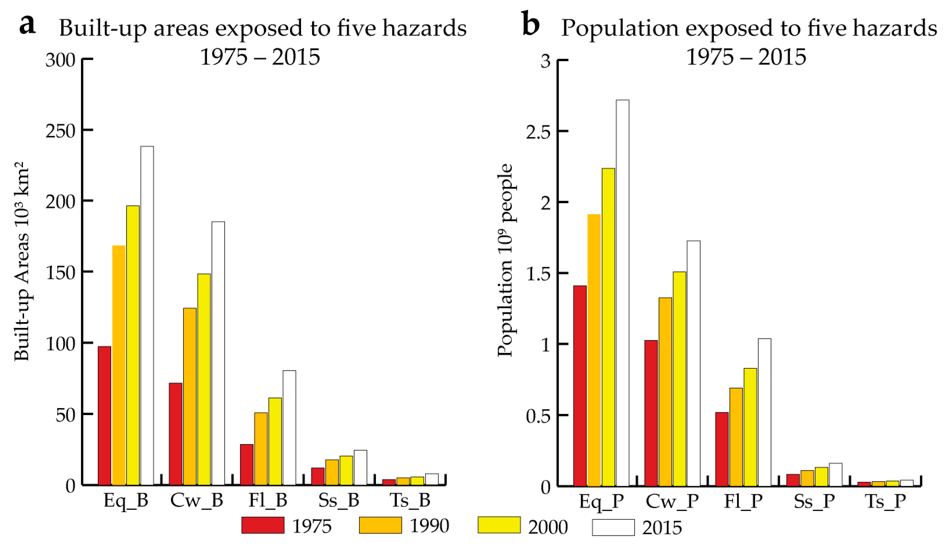
3.1. Global Exposure Statistics
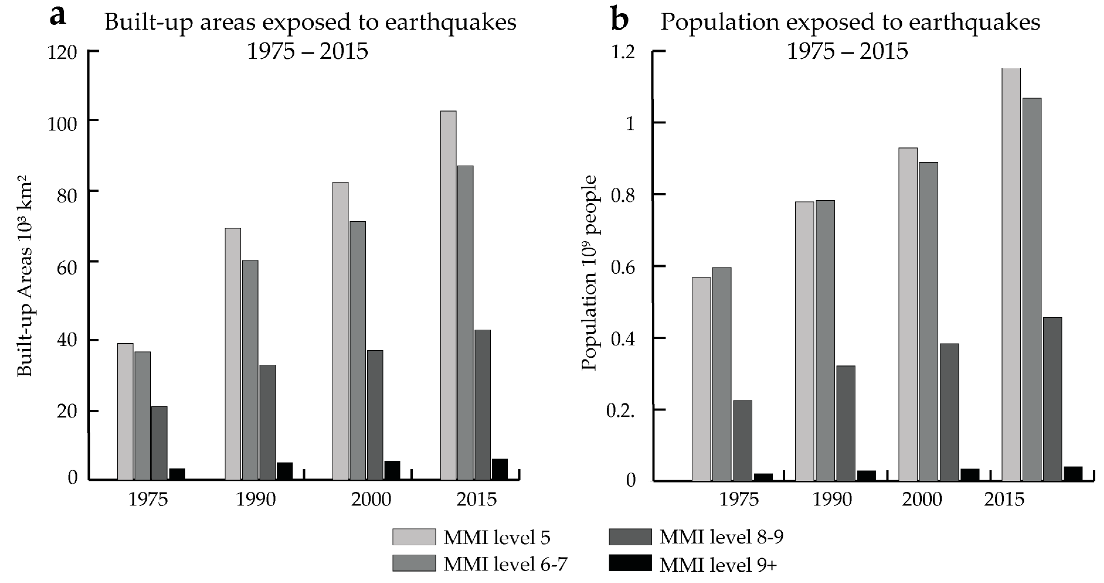
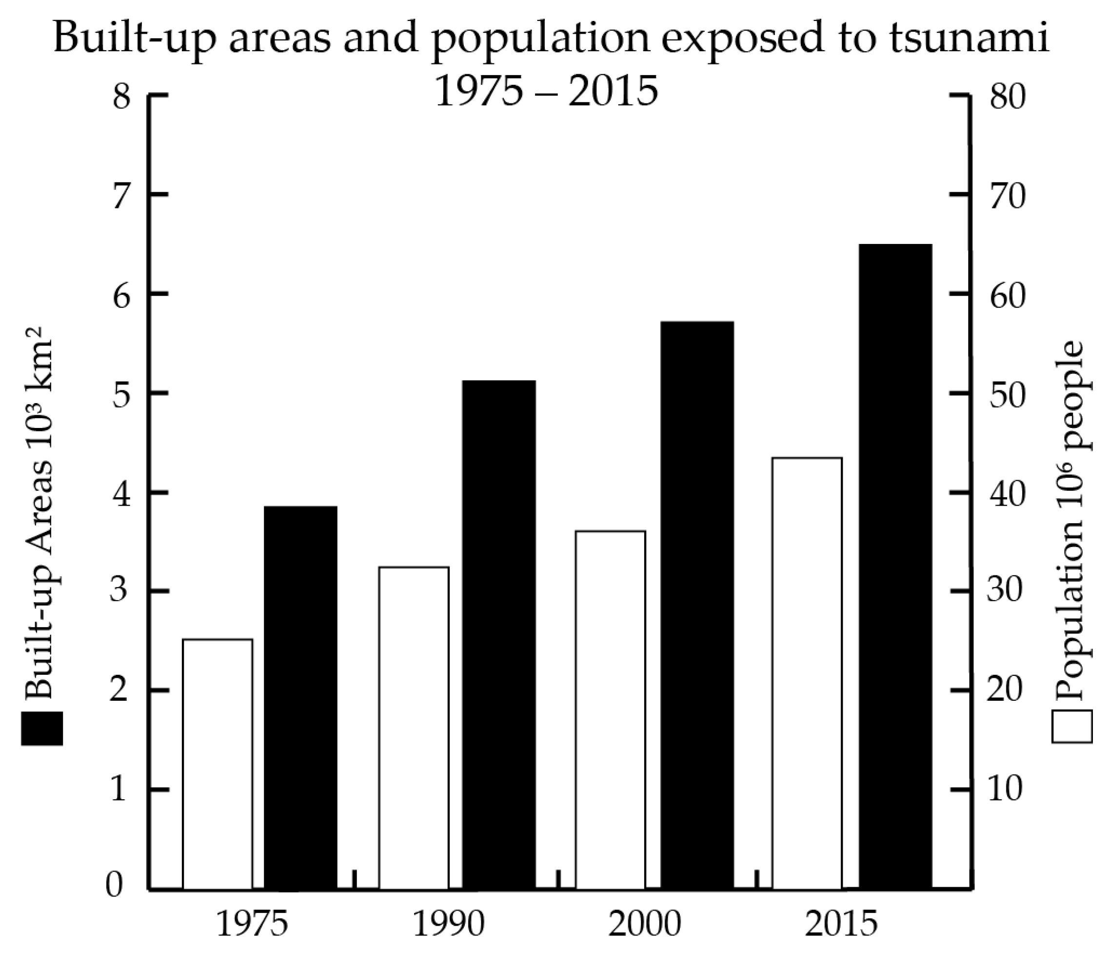
3.1.1. Exposure to Earthquakes and Tsunamis
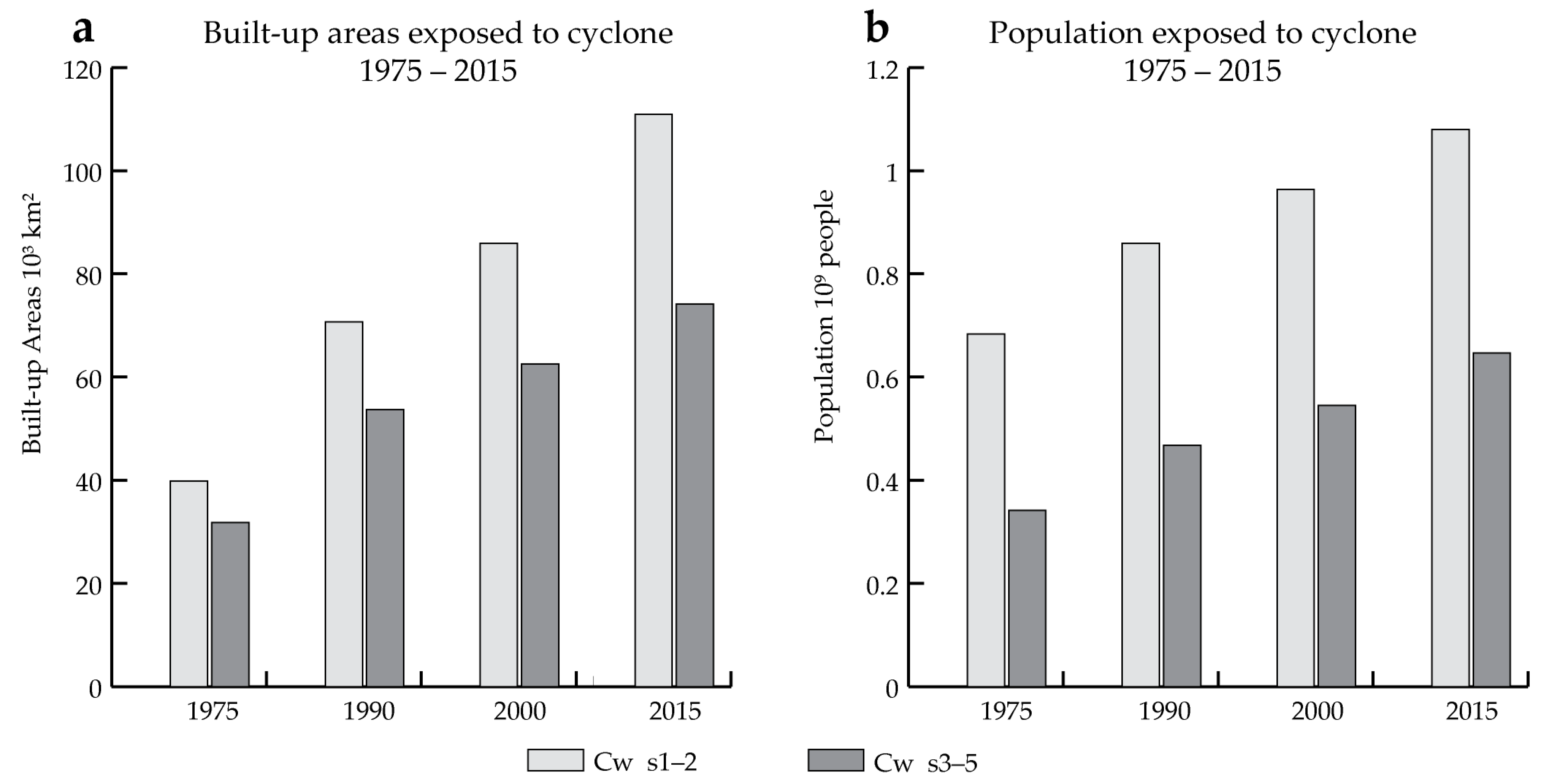
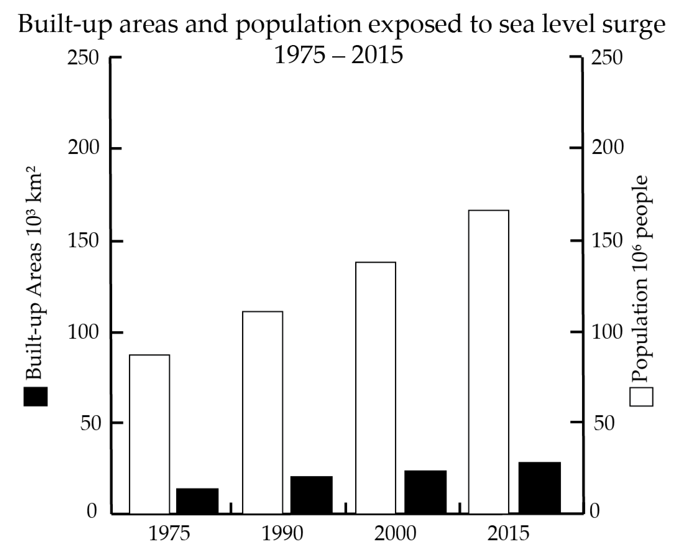
3.1.2. Exposure to Cyclone Winds and Sea Level Surge
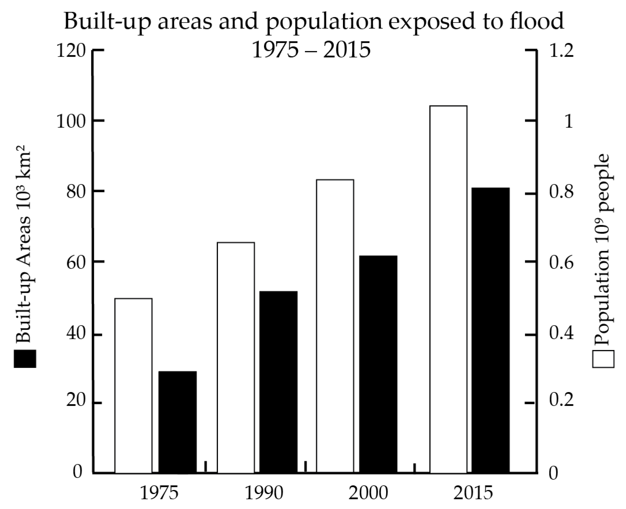
3.1.3. Exposure to Floods
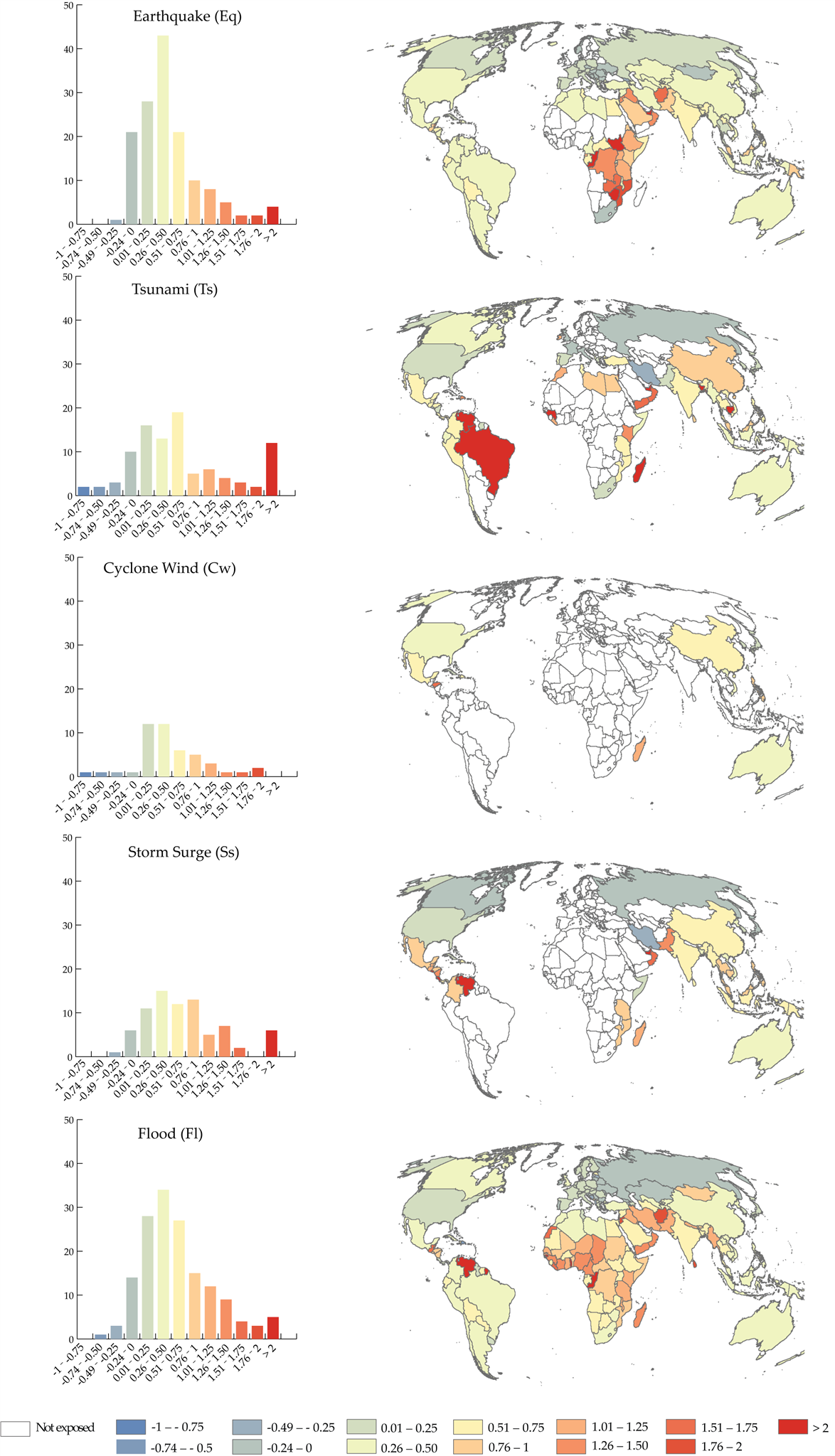
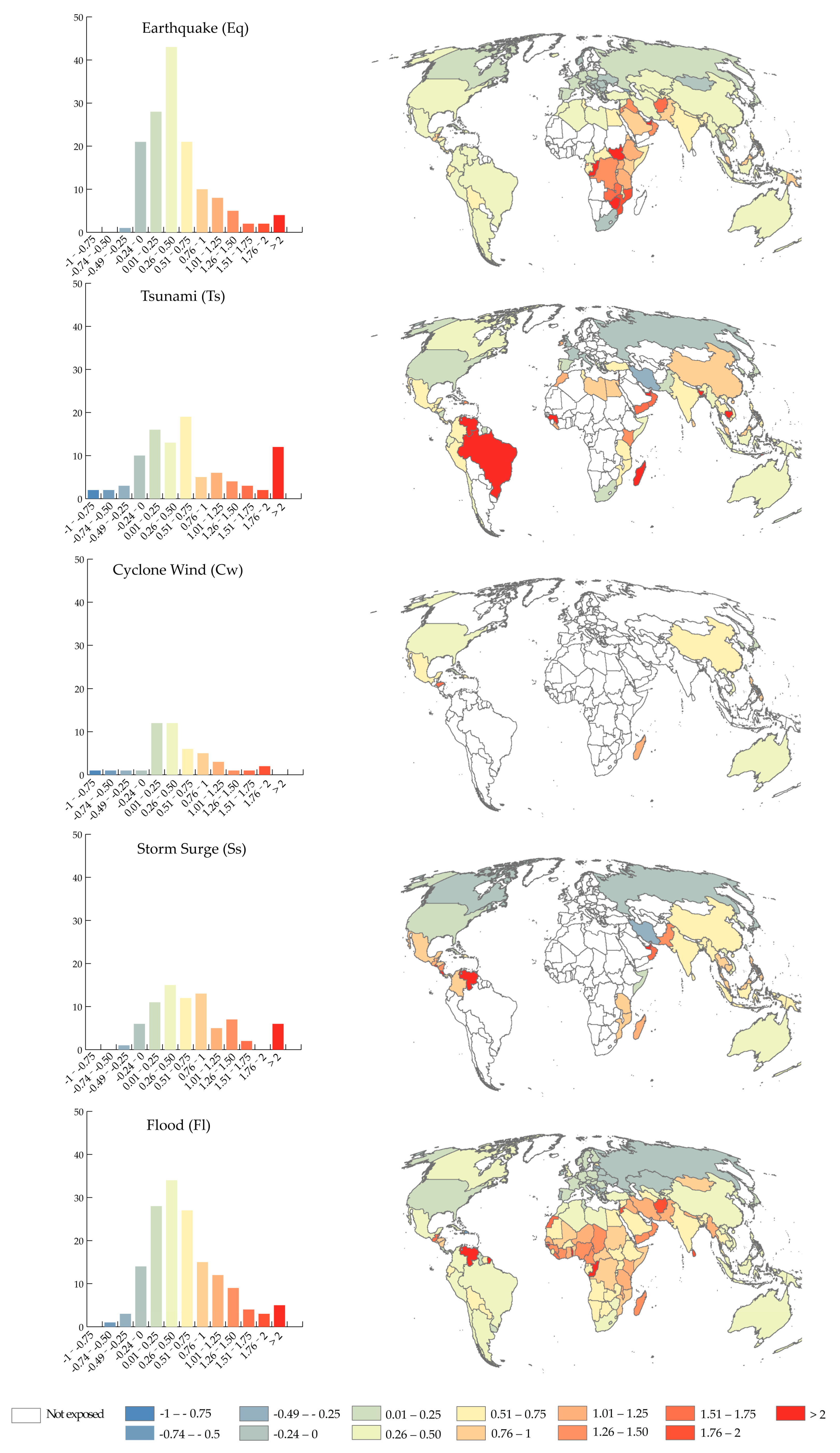
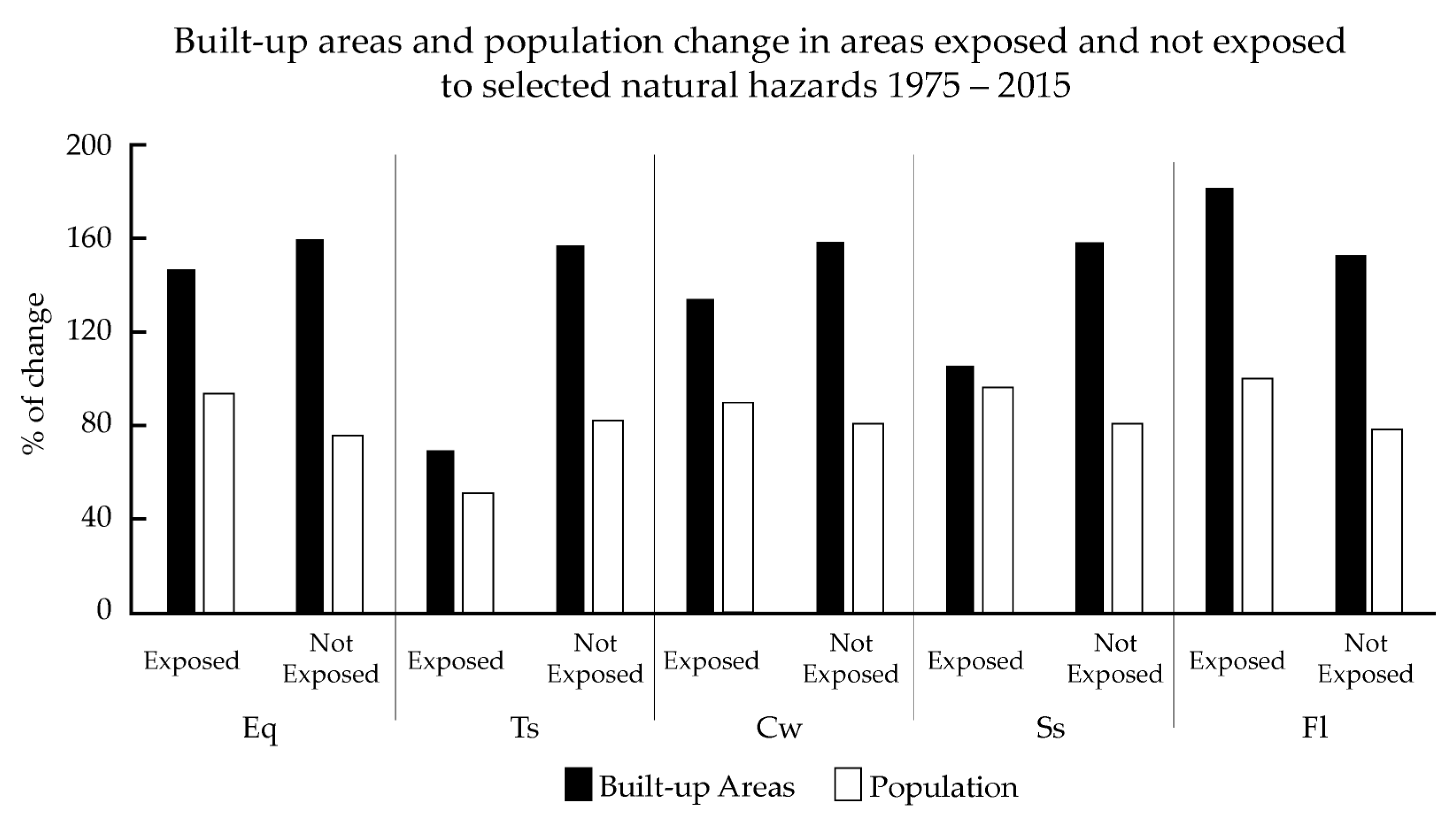
3.2. Spatio-Temporal Trends in Exposure
4. Discussion
5. Conclusions
Author Contributions
Funding
Conflicts of Interest
References
- United Nations Office for Disaster Risk Reduction (UNISDR). Global Assessment Report 2015; United Nations: Geneva, Switzerland, 2015. [Google Scholar]
- United Nations Office for Disaster Risk Reduction (UNISDR). Sendai Framework for Disaster Risk Reduction 2015–2030; United Nations International Strategy for Disaster Risk Reduction: Geneva, Switzerland, 2015. [Google Scholar]
- United Nations Treaty Collection “Paris Agreement”, Chapter XXVII 7.d. Available online: https://treaties.un.org/doc/Treaties/2016/02/20160215%2006-03%20PM/Ch_XXVII-7-d.pdf (accessed on 12 December 2015).
- United Nations. Habitat III New Urban Agenda; United Nations: Geneva, Switzerland, 2016. [Google Scholar]
- Cardona, O.D.; van Aalst, M.K.; Birkmann, J.; Fordham, M.; McGregor, G.; Perez, R.; Pulwarty, R.S.; Schipper, E.L.F.; Sinh, B.T.; Decamps, H.; et al. Determinants of risk: Exposure and vulnerability. In Managing the Risks of Extreme Events and Disasters to Advance Climate Change Adaptation; Cambridge University Press: Cambridge, UK, 2012; pp. 65–108. [Google Scholar]
- Turner, B.L.; Kasperson, R.E.; Matson, P.A.; McCarthy, J.J.; Corell, R.W.; Christensen, L.; Eckley, N.; Kasperson, J.X.; Luers, A.; Martello, M.L.; et al. A framework for vulnerability analysis in sustainability science. Proc. Natl. Acad. Sci. USA 2003, 100, 8074–8079. [Google Scholar] [CrossRef] [PubMed]
- Ehrlich, D.; Kemper, T.; Blaes, X.; Soille, P. Extracting building stock information from optical satellite imagery for mapping earthquake exposure and its vulnerability. Nat. Hazards 2013, 68, 79–95. [Google Scholar] [CrossRef]
- Dilley, M.; Chen, R.S.; Deichmann, U.; Lam, A.L.L.; Arnold, M. Natural Disaster Hotspots A Global Risk Analysis; World Bank: Washington, DC, USA, 2005. [Google Scholar]
- Loveland, T.R.; Reed, B.C.; Brown, J.F.; Ohlen, D.O.; Zhu, Z.; Yang, L.; Merchant, J.W. Development of a global land cover characteristics database and IGBP DISCover from 1 km AVHRR data. Int. J. Remote Sens. 2000, 21, 1303–1330. [Google Scholar] [CrossRef]
- Sutton, P.; Roberts, D.; Elvidge, C.; Baugh, K. Census from Heaven: An estimate of the global human population using night-time satellite imagery. Int. J. Remote Sens. 2001, 22, 3061–3076. [Google Scholar] [CrossRef]
- Schneider, A.; Friedl, M.A.; Potere, D. Mapping global urban areas using MODIS 500-m data: New methods and datasets based on ‘urban ecoregions’. Remote Sens. Environ. 2010, 114, 1733–1746. [Google Scholar] [CrossRef]
- Esch, T.; Marconcini, M.; Felbier, A.; Roth, A.; Heldens, W.; Huber, M.; Schwinger, M.; Taubenböck, H.; Müller, A.; Dech, S. Urban Footprint Processor—Fully Automated Processing Chain Generating Settlement Masks from Global Data of the TanDEM-X Mission. IEEE Geosci. Remote Sens. Lett. 2013, 10, 1617–1621. [Google Scholar] [CrossRef]
- Gong, P.; Wang, J.; Yu, L.; Zhao, Y.C.; Zhao, Y.Y.; Liang, L.; Niu, Z.; Huang, X.; Fu, H.; Liu, S.; et al. Finer resolution observation and monitoring of global land cover: First mapping results with Landsat TM and ETM+ data. Int. J. Remote Sens. 2013, 34, 2607–2654. [Google Scholar] [CrossRef]
- World Bank. East Asia’s Changing Urban Landscape: Measuring a Decade of Spatial Growth; World Bank: Washington, DC, USA, 2015. [Google Scholar]
- Srinivasan, V.; Seto, K.C.; Emerson, R.; Gorelick, S.M. The impact of urbanization on water vulnerability: A coupled human–environment system approach for Chennai, India. Glob. Environ. Chang. 2013, 23, 229–239. [Google Scholar] [CrossRef]
- Mertes, C.M.; Schneider, A.; Sulla-Menashe, D.; Tatem, A.J.; Tan, B. Detecting change in urban areas at continental scales with MODIS data. Remote Sens. Environ. 2015, 158, 331–347. [Google Scholar] [CrossRef]
- Taubenböck, H.; Esch, T.; Felbier, A.; Wiesner, M.; Roth, A.; Dech, S. Monitoring urbanization in mega cities from space. Remote Sens. Environ. 2012, 117, 162–176. [Google Scholar] [CrossRef]
- Melchiorri, M.; Florczyk, A.; Freire, S.; Schiavina, M.; Pesaresi, M.; Kemper, T. Unveiling 25 Years of Planetary Urbanization with Remote Sensing: Perspectives from the Global Human Settlement Layer. Remote Sens. 2018, 10, 768. [Google Scholar] [CrossRef]
- Ban, Y.; Gong, P.; Giri, C. Global land cover mapping using Earth observation satellite data: Recent progresses and challenges. ISPRS J. Photogramm. Remote Sens. 2015, 103, 1–6. [Google Scholar] [CrossRef]
- Riedel, I.; Guéguen, P.; Mura, M.D.; Pathier, E.; Leduc, T.; Chanussot, J. Seismic vulnerability assessment of urban environments in moderate-to-low seismic hazard regions using association rule learning and support vector machine methods. Nat. Hazards 2015, 76, 1111–1141. [Google Scholar] [CrossRef]
- Sahar, L.; Muthukumar, S.; French, S.P. Using Aerial Imagery and GIS in Automated Building Footprint Extraction and Shape Recognition for Earthquake Risk Assessment of Urban Inventories. IEEE Trans. Geosci. Remote Sens. 2010, 48, 3511–3520. [Google Scholar] [CrossRef]
- Sarabandi, P.; Kiremidjian, A.S. Development of Algorithms for Building Inventory Compilation through Remote Sensing and Statistical Inferencing; John A. Blume Earthquake Envineering Center, Standford University: Standford, CA, USA, 2007. [Google Scholar]
- Geiß, C.; Taubenböck, H. One step back for a leap forward: Toward operational measurements of elements at risk. Nat. Hazards 2017, 86, 1–6. [Google Scholar] [CrossRef]
- Wieland, M.; Pittore, M.; Parolai, S.; Zschau, J. Exposure Estimation from Multi-Resolution Optical Satellite Imagery for Seismic Risk Assessment. ISPRS Int. J. Geo-Inf. 2012, 1, 69–88. [Google Scholar] [CrossRef]
- Wieland, M.; Pittore, M.; Parolai, S.; Tyagunov, S. A Multiscale Exposure Model for Seismic Risk Assessment in Central Asia. Seismol. Res. Lett. 2015, 86, 210–222. [Google Scholar] [CrossRef]
- Wieland, M.; Pittore, M.; Parolai, S.; Zschau, J.; Moldobekov, B.; Begaliev, U. Estimating building inventory for rapid seismic vulnerability assessment: Towards an integrated approach based on multi-source imaging. Soil Dyn. Earthq. Eng. 2012, 36, 70–83. [Google Scholar] [CrossRef]
- Wieland, M.; Pittore, M.; Parolai, S.; Begaliev, U.; Yasunov, P.; Niyazov, J.; Tyagunov, S.; Moldobekov, B.; Saidiy, S.; Ilyasov, I.; et al. Towards a cross-border exposure model for the Earthquake Model Central Asia. Ann. Geophys. 2015, 58, 1–8. [Google Scholar]
- Geiß, C.; Schauß, A.; Riedlinger, T.; Dech, S.; Zelaya, C.; Guzmán, N.; Hube, M.A.; Arsanjani, J.J.; Taubenböck, H. Joint use of remote sensing data and volunteered geographic information for exposure estimation: Evidence from Valparaíso, Chile. Nat. Hazards 2017, 86, 81–105. [Google Scholar] [CrossRef]
- Pesaresi, M.; Ehrlich, D.; Ferri, S.; Florczyk, A.; Carneiro, F.S.M.; Halkia, S.; Julea, A.M.; Kemper, T.; Soille, P.; Syrris, V. Operating Procedures for the Production of the Global Human Settlement Layer from Landsat Data of the Epochs 1975, 1990, 2000, and 2014; Joint Research Centre, Publications Office of the European Union: Luxembourg, 2016. [Google Scholar]
- Pesaresi, M.; Syrris, V.; Julea, A. Analyzing big remote sensing data via symbolic machine learning. In Proceedings of the 2016 Conference on Big Data from Space, Santa Cruz de Tenerife, Spain, 15–17 March 2016; pp. 156–159. [Google Scholar]
- Sergio, F.; MacManus, K.; Pesaresi, M.; Doxsey-Whitfield, E.; Mills, J. Development of new open and free multi-temporal global population grids at 250 m resolution. In Proceedings of the AGILE 2016, Helsinki, Finland, 14–17 June 2016. [Google Scholar]
- Pesaresi, M.; Corbane, C.; Julea, A.; Florczyk, A.; Syrris, V.; Soille, P. Assessment of the Added-Value of Sentinel-2 for Detecting Built-up Areas. Remote Sens. 2016, 8, 299. [Google Scholar] [CrossRef]
- Pesaresi, M.; Ehrlich, D.; Kemper, T.; Siragusa, A.; Florczyk, A.; Freire, S.; Corbane, C. Atlas of the Human Planet 2017: Global Exposure to Natural Hazards; Joint Research Centre, Publications Office of the European Union: Luxembourg, 2017. [Google Scholar]
- Markham, B.L.; Helder, D.L. Forty-year calibrated record of earth-reflected radiance from Landsat: A review. Remote Sens. Environ. 2012, 122, 30–40. [Google Scholar] [CrossRef]
- Woodcock, C.E.; Strahler, A.H. The factor of scale in remote sensing. Remote Sens. Environ. 1987, 21, 311–332. [Google Scholar] [CrossRef]
- Gutman, G.; Huang, C.; Chander, G.; Noojipady, P.; Masek, J. Assessment of the NASA-USGS Global Land Survey (GLS) datasets. Remote Sens. Environ. 2013, 134, 249–265. [Google Scholar] [CrossRef]
- Lu, D.; Weng, Q. A survey of image classification methods and techniques for improving classification performance. Int. J. Remote Sens. 2007, 28, 823–870. [Google Scholar] [CrossRef]
- Pesaresi, M.; Syrris, V.; Julea, A. A new method for Earth Observation Data analyitics based on symbolic Machine learning. Remote Sens. 2016, 8, 399. [Google Scholar] [CrossRef]
- Center for International Earth Science Information Network-CIESIN-Columbia University. Gridded Population of the World, Version 4 (GPWv4): Population Count, Revision 10; NASA Socioeconomic Data and Applications Center (SEDAC): Palisades, NY, USA, 2017.
- Balk, D.L.; Deichmann, U.; Yetman, G.; Pozzi, F.; Hay, S.I.; Nelson, A. Determining Global Population Distribution: Methods, Applications and Data. In Advances in Parasitology; Elsevier: New York, NY, USA, 2006; Volume 62, pp. 119–156. [Google Scholar]
- Doxsey-Whitfield, E.; Macmanus, K.; Adamo, S.B.; Baptista, S.R. Taking Advantage of the Improved Availability of Census Data: A First Look at the Gridded Population of the World, Version 4. Pap. Appl. Geogr. 2015, 1, 226–234. [Google Scholar] [CrossRef]
- Giardini, D.; Grünthal, G.; Shedlock, K.M.; Zhang, P. The GSHAP Global Seismic Hazard Map. Ann. Geophys. 1999, 42, 1233–1239. [Google Scholar]
- Wald, D.J.; Quitoriano, V.; Heaton, T.H.; Kanamori, H. Relationships between Peak Ground Acceleration, Peak Ground Velocity, and Modified Mercalli Intensity in California. Earthq. Spectra 1999, 15, 557–564. [Google Scholar] [CrossRef]
- Jarvis, A.; Reuter, H.I.; Guevara, E. Hole-Filled SRTM for the Globe Version 4. Available online: http://srtm.csi.cgiar.org (accessed on 1 June 2018).
- Hoque, M.M.A.; Khan, S.A.M. Storm surge flooding in Chittagong city and associated risks. In Proceedings of the Destructive Water: Water-Caused Natural Disasters, Their Abatement and Control, Anaheim, CA, USA, 24–28 June 1996. [Google Scholar]
- Dottori, F.; Salamon, P.; Bianchi, A.; Alfieri, L.; Hirpa, F.A.; Feyen, L. Development and evaluation of a framework for global flood hazard mapping. Adv. Water Resour. 2016, 94, 87–102. [Google Scholar] [CrossRef]
- Hall, J.W.; Sayers, P.B.; Dawson, R.J. National-scale Assessment of Current and Future Flood Risk in England and Wales. Nat. Hazards 2005, 36, 147–164. [Google Scholar] [CrossRef]
- Centre for Research on the Epidemeology of Disasters and United Nations International Strategy for Diasaster Reduction. The Human Cost of Weather Related Disasters; Universite’ Catolique de Louvain: Brussels, Belgium, 2015. [Google Scholar]
- Leyk, S.; Uhl, J.H.; Balk, D.; Jones, B. Assessing the accuracy of multi-temporal built-up land layers across rural-urban trajectories in the United States. Remote Sens. Environ. 2018, 204, 898–917. [Google Scholar] [CrossRef] [PubMed]
- Klotz, M.; Kemper, T.; Geiß, C.; Esch, T.; Taubenböck, H. Mapping spatial settlement patterns on a global scale: Multi-scale cross-comparison of new and existing global urban maps. Remote Sens. Environ. 2015, 178, 191–212. [Google Scholar] [CrossRef]
- Florczyk, A.J.; Melchiorri, M.; Politis, P.; Pesaresi, M.; Esch, T.; Ehrlich, D. Analysing Global Consensus on Mapping Human Settlements and Built-Up Area from Space. In Proceedings of the 7-th Digital Earth Summit, El Jadida, Morocco, 17–19 April 2018; pp. 97–102. [Google Scholar]
- Dell’Acqua, F.; Gamba, P.; Jaiswal, K. Spatial aspects of building and population exposure data and their implications for global earthquake exposure modeling. Nat. Hazards 2013, 68, 1291–1309. [Google Scholar] [CrossRef]
- UN General Assembly. Transforming Our World: The 2030 Agenda for Sustainable Development; United Nations: Geneva, Switzerland, 2015. [Google Scholar]


| Natural Hazard | Input Dataset | Source | Semantic Content | Hazard Processing Rules Applied (Resampled to Mollweide Projection 250 m Grid Cells) | Input Data Type | RP (Years) |
|---|---|---|---|---|---|---|
| Earthquake | MMI-GSHAP | GAR 2013 | Modified Mercalli Intensity (MMI) scale | Classification 1–8; (1) hazard mask: x ≥ 5 | Raster, 6 arc-min (~11 km) WGS-84 | 475 |
| Tsunami | Tsunami Run-up | GAR 2015 | Areas potentially affected by tsunami run-up | Binary map [0, 1]; (1) hazard mask: x > 0 | Vector, 31.5 arc-sec (~1 km) WGS-84 | 500 |
| Flood | Flood map | JRC Global Flood Awareness System GloFAS | Extent of flooded areas (water depth 10 cm or more) | Depth of the flood [m]: x ≥ 0.01 (1) hazard mask: x > 0 | Raster, 30 arc-sec (~1 km) WGS-84 | 100 |
| Cyclone Wind | JRC-GAR, wind category | GAR 2015, adapted by JRC | Wind speed from Saffir-Simpson Hurricane Wind Scale | Classification 1–5; (1) reclassify into hazard zones SS1-2 and SS3-5 | Raster, 30 arc-sec (~1 km) WGS-84 | 250 |
| Cyclone Storm Surge | JRC-GAR, inundated area | GAR 2015, adapted by JRC | Areas potentially inundated by storm surge | (1) the inundated areas based on point sea-level surge and elevation SRTM v4.1; (2) hazard map from x > 0 | Vector (point), WGS-84 | 250 |
| Hazards | Exposed Built-Up Areas per Hazard (103 km2) | Exposed Population per Hazard (106 People) | ||||||
|---|---|---|---|---|---|---|---|---|
| 1975 | 1990 | 2000 | 2015 | 1975 | 1990 | 2000 | 2015 | |
| Earthquake (Eq) | 97.3 | 168.3 | 196.5 | 238.2 | 1409.3 | 1911.9 | 2235.7 | 2717.8 |
| Cyclone Wind (Cw) | 71.6 | 124.3 | 148.4 | 185.1 | 1025.2 | 1326.4 | 1508.1 | 1726.3 |
| Flood (Fl) | 28.6 | 50.8 | 61.2 | 80.4 | 518.0 | 690.4 | 828.2 | 1037.2 |
| Storm Surge (Ss) | 11.9 | 17.6 | 20.3 | 24.3 | 82.6 | 109.7 | 132.6 | 161.5 |
| Tsunami (Ts) | 3.9 | 5.1 | 5.7 | 6.5 | 27.6 | 31.8 | 36.5 | 41.7 |
| Frequency Change Class (%) | Earthquake (Eq) | Tsunami (Ts) | Cyclone Wind (Cw) | Storm Surge (Ss) | Floods (Fl) |
|---|---|---|---|---|---|
| −100–75 | 0 | 2 | 1 | 0 | 0 |
| −75–50 | 0 | 2 | 1 | 0 | 1 |
| −50–25 | 1 | 3 | 1 | 1 | 3 |
| −25–0 | 21 | 10 | 1 | 6 | 14 |
| 0–25 | 28 | 16 | 12 | 11 | 28 |
| 25–50 | 43 | 13 | 12 | 15 | 34 |
| 50–75 | 21 | 19 | 6 | 12 | 27 |
| 75–100 | 10 | 5 | 5 | 13 | 15 |
| 100–125 | 8 | 6 | 3 | 5 | 12 |
| 125–150 | 5 | 4 | 1 | 7 | 9 |
| 150–175 | 2 | 3 | 1 | 2 | 4 |
| 175–200 | 2 | 2 | 2 | 0 | 3 |
| >200 | 4 | 12 | 0 | 6 | 5 |
| Number of countries accounting exposed population | 145 | 97 | 46 | 78 | 155 |
© 2018 by the authors. Licensee MDPI, Basel, Switzerland. This article is an open access article distributed under the terms and conditions of the Creative Commons Attribution (CC BY) license (http://creativecommons.org/licenses/by/4.0/).
Share and Cite
Ehrlich, D.; Melchiorri, M.; Florczyk, A.J.; Pesaresi, M.; Kemper, T.; Corbane, C.; Freire, S.; Schiavina, M.; Siragusa, A. Remote Sensing Derived Built-Up Area and Population Density to Quantify Global Exposure to Five Natural Hazards over Time. Remote Sens. 2018, 10, 1378. https://doi.org/10.3390/rs10091378
Ehrlich D, Melchiorri M, Florczyk AJ, Pesaresi M, Kemper T, Corbane C, Freire S, Schiavina M, Siragusa A. Remote Sensing Derived Built-Up Area and Population Density to Quantify Global Exposure to Five Natural Hazards over Time. Remote Sensing. 2018; 10(9):1378. https://doi.org/10.3390/rs10091378
Chicago/Turabian StyleEhrlich, Daniele, Michele Melchiorri, Aneta J. Florczyk, Martino Pesaresi, Thomas Kemper, Christina Corbane, Sergio Freire, Marcello Schiavina, and Alice Siragusa. 2018. "Remote Sensing Derived Built-Up Area and Population Density to Quantify Global Exposure to Five Natural Hazards over Time" Remote Sensing 10, no. 9: 1378. https://doi.org/10.3390/rs10091378
APA StyleEhrlich, D., Melchiorri, M., Florczyk, A. J., Pesaresi, M., Kemper, T., Corbane, C., Freire, S., Schiavina, M., & Siragusa, A. (2018). Remote Sensing Derived Built-Up Area and Population Density to Quantify Global Exposure to Five Natural Hazards over Time. Remote Sensing, 10(9), 1378. https://doi.org/10.3390/rs10091378