Abstract
In recent years, alternating periods of floods and droughts, possibly related to climate change and/or human activity, have occurred in the Liao River Basin of China. To monitor and gain a deep understanding of the frequency and severity of the hydro-meteorological extreme events in the Liao River Basin in the past 30 years, the total storage deficit index (TSDI) is established by the Gravity Recovery and Climate Experiment (GRACE)-based terrestrial water storage anomalies (TWSAs) and the general regression neural network (GRNN)-predicted TWSA. Results indicate that the GRNN model trained with GRACE-based TWSA, model-simulated soil moisture, and precipitation observations was optimal, and the correlation coefficient and the root mean square error (RMSE) of the predicted TWSA and GRACE TWSA for the testing period equal 0.90 and 18 mm, respectively. The drought and flood conditions monitored by the TSDI were consistent with those of previous studies and records. The extreme climate events could indirectly reflect the status of the regional hydrological cycle. By monitoring the extreme climate events in the study area with TSDI, which was based on the TWSA of GRACE and GRNN, the decision of water resource management in the Liao River Basin could be made reasonably.
1. Introduction
The Liao River Basin in China is characterized by an arid and semi-arid climate [1]. Rainfall in the area mainly occurs in July or August [2,3,4]. The Liao River Basin, affected by the alternating effects of warm and moist air in the Southeast Pacific and cold air from the west or north, is prone to rainstorms [5]. Rainstorms account for a large proportion of annual precipitation, and cause frequent flooding in the basin. Moreover, the river basin suffers from different degrees of drought intensity nearly each year; spring drought is particularly severe [6]. These hazards harm the national economy, human life, and property. The frequency of hydro-meteorological extreme events has increased substantially due to global warming and high-intensity human activity, such as deforestation and unsustainable use of water resources [1,7,8,9]. Hence, a need is created to monitor and/or predict occurrences of drought and flood timely and effectively.
Total water storage change (TWSC) integrates the change of water storage in the vertical direction and includes variations in groundwater storage (GWS), soil moisture storage (SMS), snow water equivalent (SWE), and biomass water content. TWSC is derived from the Gravity Recovery and Climate Experiment (GRACE) total water storage anomalies (TWSAs) by default with a monthly temporal resolution. TWSC represents the difference in TWS (i.e., water flux) between two consecutive months, while TWSA is the anomaly with relative to the average during the time period. As a result, the GRACE satellites can be used to monitor floods and droughts by analyzing temporal variations in TWSC [10,11,12,13,14,15,16]. Droughts and floods in the Liao River Basin are mostly analyzed by statistical data of disasters in Liaoning Province, which may prove difficult to acquire. As an alternative, we used GRACE TWSAs to monitor droughts and floods.
The Earth is a dynamic system that changes over time and space. The changes in the Earth’s gravitational field are mainly caused by the Earth’s mass redistribution. GRACE is established on the basis of the time-varying gravity field of the Earth [17,18]. The GRACE satellite adopted a low-low satellite to satellite tracking technology to launch two low-orbit satellites simultaneously that are approximately 220 km apart on the same orbit. The satellite-borne GPS receiver was used to determine the orbit position of the two low-orbit satellites accurately; then, the k-band ranging system was utilized to continuously monitor the distance variation between the two satellites; thus, the change in the Earth’s gravitational field was obtained [19]. By removing the effects of tidal (solid, oceanic, and polar) and non-tidal (atmospheric and oceanic) influences, in terms of land areas, GRACE time-varying gravity fields mainly reflect the changes in Terrestrial Water Storage (TWS) on a seasonal or short time scale [20].
Low-pass filtering is required to reduce high-frequency noise in processing the GRACE spherical harmonic coefficient product. Low-pass filtering (e.g., truncation, destriping and Gaussian smoothing), however, may cause partial signal loss, which can be restored by two signal restoration methods [21]: The first is based on TWS derived from land surface models (LSMs), e.g., an additive correction approach [22,23] and scaling factor [24,25,26]; the other is less dependent on LSMs, such as forward modeling [21,27] and multiplicative correction approaches [28]. The multiplicative correction approach, however, needs to assume that the distribution of TWS changes is uniform, if not, large biases are introduced. The recently released Jet Propulsion Laboratory (JPL) mass concentration block (mascon) solutions is based on a priori constraints in space and time without additional destriping filter, thereby minimizing the effect of measurement and leakage errors [29]. The mascons can be applied at regional to global scales and do not require prior information provided by LSMs to restore signal loss [30,31]. Hence, both the JPL mascon solutions and GRACE spherical harmonic coefficient products are used here.
Drought monitoring systems require (near) real-time inputs of GRACE TWS changes; in addition, developing a drought index requires a long-term time series of data (more than 30 years) [32]. Monthly GRACE satellite data, however, are only available since April 2002, with a latency of two to six months [13]. Moreover, the first generation GRACE satellites stopped functioning before the launch of the GRACE follow-on mission in May 2018. Therefore, a method to extend the time series is required.
By assimilating the information obtained from remote sensing into the hydrological model, the integrated soil moisture (SM) can be obtained, and then the monitoring of floodplain inundations can be completed [33,34,35]. However, the vertical accuracy and spatial resolution of remote sensing images constrained the use of this method. Pan et al. [36] combined the terrestrial water budget estimated from different data sources, including in situ observations, remote sensing retrievals, LSM simulations, and global re-analyses, to enforce the water balance constraint of 32 globally distributed major basins from 1984 to 2016 using data assimilation techniques. In his article, TWS beyond the GRACE period is estimated by the variable infiltration capacity (VIC) model, which lacks GWS change and is arguably ill-suited to simulate the interactions between water storage compartments. Long et al. [13] reconstructed the GRACE TWSA data for a large karst plateau in Southwest China over the past three decades by developing an artificial neural network (ANN) model and combining this model with the monthly mean temperature, monthly precipitation and SMS to obtain the frequency and severity of droughts and floods. Sun [37] predicted the groundwater level changes by developing an ANN and combining it with GRACE products. However, the convergence rate of the ANN algorithm is slow and is prone to over-fitting. In comparison with ANN, a general regression neural network (GRNN) is superior to ANN network in terms of learning speed, function approximation, pattern recognition and classification ability [38].
GRNN demonstrates a strong nonlinear mapping capability, flexible network structure and high degree of fault tolerance and robustness [39]. The prediction effect also performs well when the sample data size is restricted, which may be exploited for unstable data processing; this effect can be used to process unstable data [40]. However, overfitting may occur with the GRNN method reconstructing TWS changes for the training period, resulting in poor performance in other periods, especially over the hindcasting period. To avoid this, cross validation is applied over the training period and early stopping is considered. This paper aims to (1) compare TWS changes of JPL mascon solutions with GRACE spherical harmonic solutions, (2) predict TWSA for the Liao River Basin in China beyond the GRACE period with GRNN models, and (3) monitor droughts and floods across the Liao River Basin with a drought index, where the total storage deficit index (TSDI), which is based on a long-term TWSA time series. The flowchart of this study is shown in Figure 1.
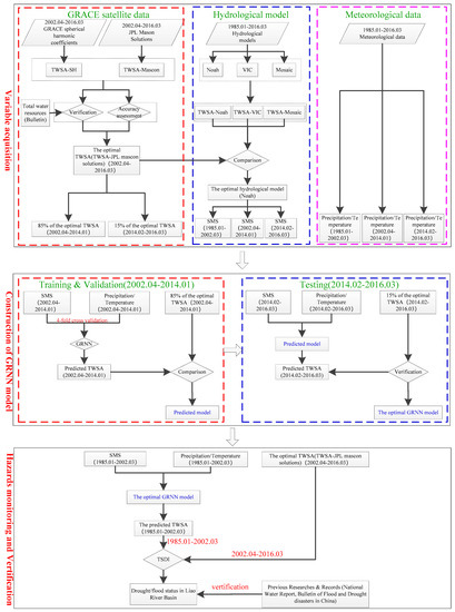
Figure 1.
Flowchart of drought and flood disaster monitoring in the Liao River Basin. Note: the time span of the hydrological model and meteorological data from January 1985 to March 2016 was divided into three parts: the first part was from January 1985 to March 2002, the second part was from April 2002 to January 2014, and the last part was from February 2014 to March 2016. By contrast, the GRACE satellite data from April 2002 to March 2016 were divided into two parts: one was from April 2002 to January 2014, and the other was from February 2014 to March 2016. The part from April 2002 to January 2014 was used for training (75%) and validating (25%) the GRNN model; during this process, 4-fold cross validation was applied. However, the part from February 2014 to March 2016 was utilized for testing the predicted model to avoid overfitting. The remaining part of the hydrological model and meteorological data, from January 1985 to March 2002, was used as the input variables of the optimal GRNN model to obtain the TWSA from January 1985 to March 2002.
2. Study Area
The Liao River originates from Guangtoushan in Qilaotu Mountain in Hebei Province and flows through Hebei Province, Inner Mongolia, Jilin Province and Liaoning Province [2,3,41]. The Liao River Basin (117°00′E–125°30′E, 40°30′N–45°10′N) is situated in the southwest of Northeast China, east of the Di’er Songhua and Yalu Rivers, west of the Inner Mongolia Plateau, south of the Luan River, Daling River Basin, and Bohai, and north of the Songhua River; the total area equals 221,100 km2 [42,43]. Figure 2 illustrates the location of the Liao River Basin and the distribution of the meteorological stations.
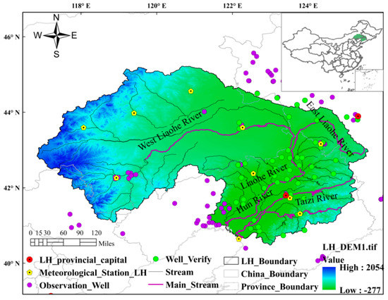
Figure 2.
Distribution map of the Liao River Basin.
The main tributaries of the Liao River Basin are the West Liao, East Liao, and Liao and Hun Tai rivers [5]. Most of the regions in this basin are characterized by a temperate semi-humid and semi-arid monsoon climate. Severity of droughts and floods is related to precipitation [6]. The frequency of droughts is high in spring due to dry weather conditions when sand winds are common. Precipitation is highly localized in summer, resulting in alternating droughts and floods. Precipitation is virtually absent in autumn and winter, which makes droughts likely to occur during these seasons [44].
3. Materials and Methods
3.1. Data and Processing
3.1.1. GRACE Data
The GRACE TWSA is derived using two solutions. The first method, namely, the traditional GRACE spherical harmonic solutions, is based on the GRACE spherical harmonic coefficient products; the second method is the JPL mascon solutions.
The GRACE spherical harmonic coefficient products are currently available in three centers: the Center for Space Research (CSR) at the University of Texas at Austin, the NASA Jet Propulsion Laboratory and the German Research Center for Geoscience. Here, we used the GRACE Level-2 RL05 data provided by the CSR and recorded from April 2002 to March 2016, covering 151 months (the data from June and July 2002; June 2003; January 2004; January and June 2011; May and October 2012; March, August, and September 2013; February, July, and December 2014; and June, October, and November 2015 are missing but can be restored by linear interpolation [26]). To reduce the error of the high-order spherical harmonic coefficient, the GRACE spherical harmonic coefficients are truncated at the maximum degree and order of 60, and the degree-one spherical harmonic coefficients (C10, C11 and S11) are replaced with those calculated by Swenson et al. [45]. The C20 coefficients in the GRACE data were replaced with Satellite Laser Ranging (SLR) C20 to reduce measurement errors [46]. The multiyear mean gravity field is subtracted from the monthly time-varying gravity fields to obtain the monthly anomalous gravity field. The north–south stripes were removed by destriping [47], and the high-frequency noise in the spherical harmonic coefficients was reduced by 300-km Gaussian smoothing. Furthermore, the TWS in the study area is obtained by applying the regional kernel function to the spherical harmonic coefficients [48]. Moreover, bias (signal lost to the surrounding area) and leakage (signal gained from the surrounding area) corrections were performed through the scaling factor method. This method computes multiple factors by least squares fitting between the filtered and unfiltered TWSA at the basin scale [25,26]. The TWSAs are then converted into TWSC in the form of equivalent water height (EWH) by deriving the TWSAs with respect to time, for example, TWSCi = (TWSA(i+1) − TWSA(i−1))/2, where i is the month during the study period [49].
Additionally, the newly released JPL mascon solutions in the form of equal-area 3-degree spherical cap are also used to obtain the TWS changes. The data represent TWS anomalies relative to the baseline average from January 2004 to December 2009. It is critical that the same time average is used while comparing with other products. At last, the TWSA is obtained by applying mascon gain factors on the mascon fields [29].
3.1.2. Hydro-Meteorological Data
(1) Statistical bulletin data
The total storage of water resources was obtained from the Water Resources Bulletin of the Song Liao River Basin from 2002 to 2016, which could be used to verify the accuracy of GRACE TWSA. The data sources of the water resources bulletin are mainly the collection and utilization of existing information in the relevant departments, supplemented by the necessary typical investigation, observation experiments and special research work [The compilation of technical outline of China Water Resources Bulletin]. The yearly anomalies of the total storage of water resources were obtained and were relative to the mean of data from 2002 to 2016. The GRACE TWSA in this study was presented on a monthly scale and expressed in the form of EWH, and the total storage of water resources provided by the bulletin was expressed on an annual scale and in volume. Therefore, to achieve a unity in them, the expression of the statistical bulletin data was converted to the form of EWH, and the time scale of GRACE TWSA was transformed into year. The GRACE TWSAs in 2002 and 2016 were not used in the comparison because data of several months in these 2 years are missing. Moreover, Grubbs statistical test [50] was used to detect outliers before the comparison between the two solutions and the statistical bulletin data. The statistical results showed that the bulletin data had a large anomaly in 2010. Therefore, the original data of 2010 will be listed separately as follows for key analysis.
(2) Meteorological data
The meteorological data (e.g., precipitation and temperature) were acquired and set as the input parameters for the following GRNN models. Daily precipitation and temperature data were gathered from the China Meteorological Data Sharing Network (URL: http://data.cma.cn/) from January 1985 to March 2016. Figure 2 illustrates the distribution of the meteorological stations in the Liao River Basin. The daily meteorological station data were interpolated by kriging; as a result, the grid daily precipitation (or temperature) was obtained. By summing all the daily precipitation (or temperature) grid data for the same month of the same year, the grid monthly precipitation (or temperature) data could be achieved. Finally, the regional precipitation (or temperature) data on a monthly scale was derived by averaging the grid monthly precipitation (or temperature). The monthly precipitation products from the Tropical Rainfall Measuring Mission (TRMM) from April 2002 to March 2016 were used to verify the reliability of the spatially averaged in situ precipitation (Figure 3). The correlation coefficient of the two sources was 0.98, and the root mean square error (RMSE) was 9 mm month-1, indicating a high consistency.
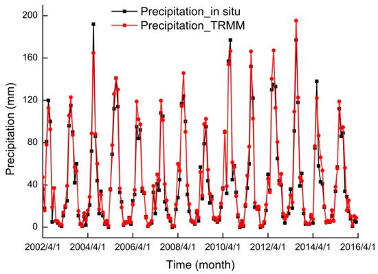
Figure 3.
Comparison between the in situ precipitation from meteorological stations and the precipitation from satellite (TRMM 3B43) over the Liao River Basin from April 2002 to March 2016.
3.1.3. Hydrological Model Data
The hydrological model has been widely used to obtain the hydrological parameters, such as SM and SWE, due to the long time span and global grid scale [13,32]. The following three hydrological models for the time span from January 1985 to March 2016 were used in this article: Noah, Mosaic and VIC from the Global Land Data Assimilation System (GLDAS) [51]. Here, the CLM model in GLDAS was not used because it considerably underestimates the amplitude of SM variations across the land surface and frequently deviates from other LSMs [31]. GLDAS can provide optimal near-real-time land surface states which come from the fusion of satellite and ground observation data, such as SM and SWE [27,31]. The model excludes the groundwater and the Antarctic data [52,53]. The processing method of the hydrological model was the same as that of the GRACE spherical harmonic coefficient products (e.g., truncation, monthly anomalies, and 300 km Gaussian smoothing). The specific processing process of the hydrological model was as follows: the grid data of hydrological models were expanded to the spherical harmonic coefficients with a maximum degree and order of 60; the monthly anomaly was calculated, which was relative to the mean of the grid data between April 2002 and March 2016, and a 300 km Gaussian smoothing was applied; the decorrelation filter was not used because no north–south stripes were observed in the hydrological model data [27]. The depths of SM recorded by Noah, Mosaic, and VIC were different, which were 2, 3.5, and 1.9 m, respectively. Here, the SMS of different hydrological models was compared with the GRACE TWSA, and the SMS that best fit the GRACE TWSA was used as the input parameter for the following GRNN models.
3.2. GRNN Model
The GRNN model demonstrates the advantages of good topology, high precision and fast convergence speed [54] and performs a nonlinear functional mapping from past observations X = (x1, x2, ..., xn)T to future values Y = (y1, y2, … yk)T. In Equation (1), F is the mapping by the GRNN, and w is the vector of all parameters [39]. Here, the GRNN model was used to predict the monthly TWSAs from January 1985 to March 2002.
The GRNN model consists of four layers, namely, input, pattern, summation, and output [40] (Figure 4). In this study, three types of predictions were set to forecast TWSAs, namely, SMS and precipitation (Prediction 1), SMS and temperature (Prediction 2), and SMS, precipitation, and temperature (Prediction 3) due to the high correlation between the GRACE TWSAs and SMS anomalies and the direct effect of precipitation on the SMS anomalies and the indirect reflection of temperature on evaporation.

Figure 4.
Structure of GRNN for predicting the monthly GRACE TWSAs from January 1985 to March 2002. The input layer xn is the combination of mean precipitation and temperature from in situ observations and SMS from the Noah hydrological model; n is the number of input variables. The output layer yk is the time series of the predicted monthly GRACE TWSA and k is the time span on a monthly scale. Pn, SD, and SNT are the neuronal transfer functions between layers.
The output of the pattern layer neurons i is the exponential form of the exponential square of the Euclidian distance square between the input variable and its corresponding learning sample X (Equation (2)). In Equation (2), Pi is the transfer function of the pattern layer neurons, X is the input variable, and Xi is the corresponding learning sample of neurons i.
Two types of neurons in the summation layer were used to conduct the summation (as expressed in Equations (3) and (4)). One way is by performing an arithmetic summation of the outputs of all the neurons in the pattern layer; the connection weight between the pattern layer and each neuron is 1. The other method is the weighted summation of all the pattern layer neurons; the connection weight between the ith and jth neurons in the pattern and summation layers, respectively. Yij is the jth element from the ith output sample. Moreover, the subscript j in Equation (4) is the time series to be predicted.
The prediction results could be retrieved by dividing the output from the summation layer (Equation (5)). The output neuron is the monthly GRACE TWSA.
However, in neural network training, overfitting may occur, that is, the prediction error of the neural network for the training set is considerably small, but the error for the testing set is considerably large. Here, earthly stopping, which divided the data sets into training, validation, and testing sets, was adopted to avoid overfitting [40].
Thus, after repeated experiments, the GRACE TWSA data from April 2002 to January 2014 (85% of all samples) were used for training (75%) and validating (25%) the GRNN model. The 4-fold cross validation method was applied during the training period. The GRACE TWSA data from February 2014 to March 2016 (15% of all samples) were used as testing set, which was mainly used to compare the simulation effects of different GRNN models. The resulting optimal GRNN model was then utilized to predict the GRACE TWSAs in the Liao River Basin from January 1985 to March 2002.
3.3. Total Storage Deficit Index (TSDI)
The meteorological disaster indexes used currently include the Palmer drought severity index (PDSI) [55], standardized precipitation index (SPI) [56], and soil moisture deficit index (SMDI) [57]. PDSI is the most widely used meteorological drought index. This index is used to evaluate long-term abnormal drought or humidity at a certain area. Moreover, PDSI assumes that the input parameters, such as land use, land coverage and soil characteristics, are uniform in the entire climate zone. The calculation process of the SPI drought index is simple but disregards the impact of temperature anomalies. SMDI is an agricultural drought index that demonstrates the advantage of high temporal and spatial resolutions. However, this index requires a high quantity and quality of SM.
Droughts or floods may occur when a dry or wet state exceeds a certain period [32]. The SMDI developed by Narasimhan and Srinivasan [57] was renamed by Yirdaw et al. [15] as the TSDI. This index can be used to describe long-term dry–wet conditions. The TWSAs derived from the GRACE satellites contain all the water storage changes, such as SWS, SMS, SWE, and GWS. The TSDI can be computed using the GRACE TWSAs and can be estimated by calculating the total storage deficit (TSD, %) [15].

Table 1.
Severity classification of TSDI drought and wetness.
4. Results
4.1. Evaluation of the GRACE TWSAs
4.1.1. Comparison between GRACE Spherical Harmonic Solutions and JPL Mascon Solutions
In this article, the acquisition of TWSA from April 2002 to March 2016 adopted two methods: GRACE spherical harmonic solutions and JPL mascon solutions. The Pearson correlation coefficient and RMSE between the two solutions were 0.83 and 18 mm, respectively, indicating a high correlation. The amplitudes of GRACE spherical harmonic-based TWSA and JPL mascon-based TWSA varied from −8.38 cm to 8.46 cm and −5.50 cm to 8.56 cm respectively. Figure 5 show that the difference in amplitude of the two methods was insignificant.
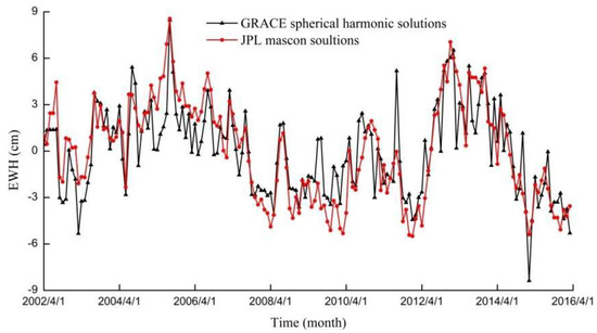
Figure 5.
TWSA of GRACE spherical harmonic solutions and JPL mascon solutions over the Liao River Basin from April 2002 to March 2016.
4.1.2. Comparison between the Two Solutions and the Statistical Bulletin Data
Prior to the prediction of the TWSAs from January 1985 to March 2002, the TWSAs of the Liao River Basin from April 2002 to March 2016, which were restored by GRACE, were verified by the water resources storage from the Water Resources Bulletin of the Song Liao River Basin [58]. Considering the special characteristics of TWSA in the Water Resources Bulletin in 2010, the TWSAs from 2003 to 2015 were divided into three parts for analysis: 2003–2009, 2010, and 2011–2015.
Table 2 and Figure 6 show that the two solutions correlated well with the statistical bulletin data for the two periods; the RMSE between the two solutions and the statistical bulletin data was small. Moreover, the difference in the RMSEs of JPL mascon solutions and the RMSEs of GRACE spherical harmonic solutions was insignificant for the same period. However, the correlation between the JPL mascon solutions and the statistical bulletin data was slightly higher than that for GRACE spherical harmonic solutions.
Table 2.
Comparison of TWSA between different GRACE solutions and the statistical bulletin data.
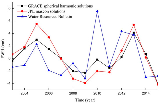
Figure 6.
Comparison between the two solutions of GRACE TWSA and the Water Resources Bulletin of the Song Liao River Basin.
Figure 6 shows that the TWSA in 2010 derived from GRACE spherical harmonic solutions and JPL mascon solutions indicated a similar change trend with the TWSA of the Water Resources Bulletin; specifically, both increased significantly in 2010 and then decreased in 2011. Combining with the precipitation in Figure 3, the precipitation showed a considerable increase in 2010; a relatively high precipitation peak in summer and also a secondary peak in spring were observed. The increased precipitation might lead to an increase in TWS in 2010.
However, the amplitude of TWSA from the Water Resources Bulletin was extremely larger than the two different GRACE solutions in 2010. The difference could be explained by the following: the precipitation in the study area was relatively high and concentrated from July 19 to August 22 in 2010. GRACE satellites measured gravity anomalies on a monthly scale and might fail to capture the moment with the maximum precipitation. However, the total water resources of the Water Resources Bulletin were obtained by a statistic of the real-time measurement data.
All of these results indicated that the TWSAs obtained from the two solutions were accurate, and the JPL mascon solution might be slightly better than the GRACE spherical harmonic solution.
4.1.3. Error Estimation
To further determine a better solution of TWSA, the uncertainty of the GRACE spherical harmonic solutions and JPL mascon solutions was estimated. The error of GRACE spherical harmonic solutions mainly includes measurement and leakage errors. The method of Chen et al. [59] was used to estimate the measurement error of GRACE, which calculates the RMS of the residual of mass variation in the ocean region that has the same latitude as the study area. In addition, the method of Landerer and Swenson [24] method was applied to obtain the leakage error. By calculating the RMS of the sum of squares of the measurement and leakage errors, the total error of GRACE spherical harmonic solutions in the study area could be derived and was 28 mm. In addition, the uncertainty of JPL mascon solutions could be obtained from the JPL website and was 23 mm in the study area.
From the uncertainty of the two solutions and the comparison with the statistical bulletin data in Section 4.1.2, we can conclude that the accuracy of JPL mascon solutions was slightly higher than that of GRACE spherical harmonic solutions. Therefore, in the following process, the JPL mascon solutions will be used to simulate the GRNN models.
4.2. Selection of the Optimal Hydrological Model
SMS derived from the hydrological models was needed in the simulation of GRNN models. Thus, selecting an optimal hydrological model that best fits the change trend of TWSA is necessary. Here, all the three hydrological models were compared with JPL mascon solutions from the perspective of correlation and amplitude, and Table 3 presents the corresponding correlation coefficients. Table 3 shows that the SMS from the Noah hydrological model demonstrated the highest correlation with the JPL mascon-based TWSA (r = 0.69), which was consistent with the result of Long et al. [13].
Table 3.
Correlation coefficients of different hydrological models and JPL mascon-based TWSA (n = 168).
Figure 7 depicts the comparison between JPL mascon-based TWSA and the SMS from different hydrological models. The three hydrological models of GLDAS and JPL mascon-based TWSA provided consistent time series changes. However, the difference in amplitude was relatively large in summer and winter. The TWSA of JPL mascon varied from −5.50 cm to 8.56 cm, whereas those of the Noah, VIC, and Mosaic hydrological models varied from −3.48 cm to 6.95 cm, −3.57 cm to 5.91 cm, and −3.44 cm to 5.86 cm, respectively. Among the amplitudes of all hydrological models, the amplitude of the Noah hydrological model was the closest to the JPL mascon solutions.
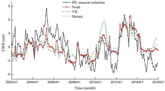
Figure 7.
Comparison between the JPL mascon-based TWSA and SMS of different hydrological models over the Liao River Basin from April 2002 to March 2016.
The SMS derived from the Noah hydrological model fits well with the JPL mascon-based TWSA whether in terms of the correlation or the amplitude. Therefore, Noah of GLDAS was the optimal hydrological model to describe the TWS changes in the study area. As a result, the SMS anomaly from Noah was selected as the input of the GRNN model.
However, the data during the period of 1995–1997 in GLDAS-1 are subject to large uncertainties due to erroneous forcing fields as described on the NASA website [60]. The time span of GLDAS-2.0 was from 1948 to 2010. Here, the SM of GLDAS-2.0 from 1985 to 2010 was selected to compare with that of GLDAS-1 (Figure 8). Figure 8 show that the SMs of GLDAS-1 and GLDAS-2 showed an opposite trend from 1995 to 1997. However, from 1985 to 1994, the correlation coefficient and RMSE of the two models were 0.68 (n = 120) and 58.69 mm, respectively. The corresponding correlation coefficient and RMSE from 1998 to 2010 were 0.79 (n = 156) and 101.41 mm, respectively. The difference between the amplitudes of the two models might be caused by the different forcing fields used in the two models. However, the overall change trends of SM in the two models were consistent except for those in 1995–1997. Thus, the SMS from Noah of GLDAS-2 during the period of 1995–1997 was used to replace that of GLDAS-1.
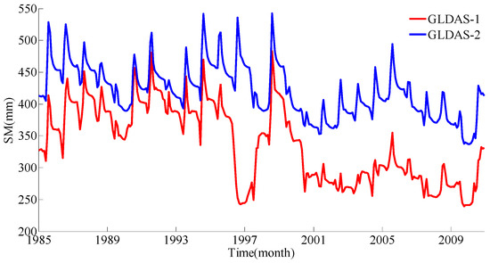
Figure 8.
SM of GLDAS-2 and GLDAS-1 over the Liao River Basin from 1985 to 2010.
4.3. Evaluation of the TWSAs Predicted by the GRNN Models
The JPL mascon-based and GRNN method-predicted TWSAs in the testing period from February 2014 to March 2016 were analyzed. Table 4 and Figure 9 present the results. The GRNN-predicted TWSAs for the testing period correlated well with the JPL mascon-based TWSAs except for the last dots. The difference in the last dots might be attributed to the trend in SMS anomalies at the corresponding location. The difference in correlation among the three prediction models in Table 4 was insignificant. Therefore, to select a reliable and stable model, the F tests on the three predictions were performed further under the significance level of 0.05. Table 4 shows that Prediction 1 had the highest F (F = 5.51). The TWSA from Prediction 1 had a high correlation (r = 0.90) (n = 26) with GRACE TWSA from February 2014 to March 2016. The RMSE between the two was 18 mm, which was lower than the uncertainty of the JPL mascon-based TWSA of 23 mm. As a result, the GRNN model of Prediction 1 was regarded as the optimal model and could be used for further analysis.
Table 4.
Accuracy assessment of TWSA predicted by GRNN models for the testing period from February 2014 to March 2016 (n = 26).

Figure 9.
JPL mascon-based TWSAs and SM anomalies (generated by GLDAS Noah) over the Liao River Basin from April 2002 to March 2016. The hollow triangles from February 2014 to March 2016 are the GRNN-generated TWSAs with three types of predictions.
4.4. Drought/Flood Status of the Liao River Basin Monitored by the TSDI
(1) Calculation of TSD and cumulative TSD
By using the TWSA time series, which was obtained from the optimal GRNN model (Prediction 1 in Table 4) and the JPL mascon solutions, and combining with Equation (6), the TSD (Figure 10) in the Liao River Basin from 1985 to 2016 was calculated. Figure 10 depicts that the TWS followed a clear downward trend from March 2000 to May 2002, and the TSD was negative from May 2000 to May 2002. The study area was relatively dry and prone to droughts from May 2000 to May 2002 because the TWS had been decreasing for more than 3 consecutive months. Assuming that May 2000 was the beginning of the dry state, the monthly cumulative TSD (red solid dot in Figure 11) could be calculated with the TSD from May 2000 to May 2002. Figure 11 describes the temporal patterns of historical droughts and wetness. The monthly cumulative TSD gradually decreased from May 2000 to May 2002 and then began to increase, thereby indicating that the dry state of the Liao River Basin had ended in May 2002.
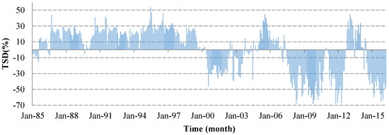
Figure 10.
TSD (%) for the Liao River Basin during the period of 1985–2016.
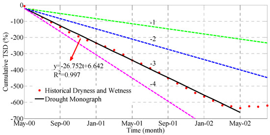
Figure 11.
Cumulative TSD of the Liao River Basin in China.
(2) Calculation of the parameters m, b, p, and q
As described in the previous section, the study area began to dry up in May 2000 and the cumulative TSD reached its maximum value in May 2002. Thus, the monthly cumulative TSD from the beginning of May 2000 to May 2002 was used to conduct linear fitting, through which the best-fitting line was obtained. The slope and intercept of the best-fitting line (black line in Figure 11) were m = −26.752 and b = 6.642, respectively.
Parameter C could be estimated from the drought monograph of the best-fitting line. The drought monograph of the Liao River Basin in China from May 2000 to May 2002 needs to be determined. In 2012, Jiang et al. [61] calculated the temporal and spatial characteristics of droughts and floods in Liaoning Province in the past 50 years using the Z index. The results indicated that the drought and flood disaster degrees in Liaoning Province in 2000, 2001, and 2002 were great drought, partial drought and partial drought respectively. In 2016, Wu et al. [62] used the meteorological drought comprehensive monitoring index to monitor the meteorological drought in Liaoning Province from 1951 to 2014. They highlighted that a strong drought occurred in 2000 and 2001 in Liaoning Province, especially in the central part. Wang et al. (2007) [63] indicated that from 1951 to 2005, a total of 55 years, the time with the largest drought coverage was 2000, reaching 68%, followed by 2002 and 2001. The greater the drought coverage, the more severe the drought. Zou et al. (2010) [64] found that the Liao River Basin had a continuous drought area exceeding 40% from 1951 to 2008, of which the drought area in 2001 reached 54.8%. Therefore, on the basis of the above-mentioned studies, the drought monograph of the drought events from May 2000 to May 2002 was defined as severe drought, with a C value of −3.
The best-fitting line of the cumulative TSD (solid black line in Figure 11) was defined as the upper limit of severe drought in the drought monograph. As the horizontal line of zero in Figure 11 represents “normal”, the interval from normal to severe was divided into three equal intervals. Moreover, the body of the graph above the best-fitting line was correspondingly divided by two dashed lines labeled “−1” (green line) and “−2” (blue line), which represent the upper limits of mild and moderate droughts. The fourth line below the best-fitting line was derived with an equal interval and labeled “−4” (magenta line), which represents the upper limits of extreme drought.
In accordance with the values of parameters m, b and C combined with Equation (8), parameters p = −0.330 and q = 0.149 could be obtained.
(3) Calculation of the TSDI
Equation (9) could be obtained by substituting parameters p and q into Equation (7). Then, the value of the TSDI for a given month in the study area could be calculated.
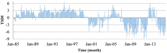
Figure 12.
Monthly TSDI of the Liao River Basin.
(4) Assessment of meteorological hazards by the TSDI
The TSDI ranged between −8.70 and 6.50 from January 1985 to March 2016 (Figure 12). For three consecutive months or over, the value of the TSDI was less than −1 or greater than 1, and then this period was defined as a drought or flood event, respectively [32]. In accordance with the previous definition, 14 flood and six drought events with different intensities and durations were detected. Table 5 lists the corresponding periods. By calculating the best-fitting line of the cumulative TSDI with different disaster events, and comparing the slope of the best-fitting line with the categorization scheme in Table 1, the disaster severity could be obtained.
Table 5.
Statistics of disaster events identified by the TSDI.
5. Discussion
5.1. Noah-Based SM versus JPL Mascon-Based TWSA
Figure 7 shows that the amplitudes of the TWSAs obtained from GRACE and Noah exhibited a certain difference, especially in mid-2014. This result could be explained from two aspects: one is that the Noah hydrological model excludes surface water and groundwater variables; the other is that the Liao River Basin suffered a severe drought in 2014, and the drought lasted until the mid-2015 [41], which resulted in severe deficit in the TWS during this period. However, the seasonal variations and trend between the TWSAs from the GRACE and Noah hydrological model agreed well and showed peaks in summer (June–August) and valleys in winter (December–February).
Figure 7 displays some systematic differences between mascon solutions and the hydrological models. The differences were mainly because the hydrological models only contained SM, which was only one component of TWS. Positive anomalies of the mascon solutions were much higher than those of the hydrological models, especially in summer, when more precipitation was observed. This case was a portion of the precipitation is converted into surface runoff, most of which is intercepted by the soil, and the infiltration is converted into soil water. Under the effect of gravity, part of the infiltration is converted into groundwater. As a result, the runoff is stored in soil water and groundwater. Thus, positive anomalies of the mascon solutions (TWS) were considerably higher than those of the hydrological models (which only contains SM).
Besides, Seasonal biases may exist in the TWSA between hydrological models and GRACE solutions [65], and may bring some systematic differences between mascon solutions and hydrological models. The biases may have some impact on the final meteorological disaster monitoring results, and we will test it in the future work.
5.2. Analysis of TSDI Results
TSDI results from January 1985 to March 2016 were divided into two parts for analysis due to the limited materials of meteorological disaster. The first part was from January 1985 to December 2000, which was compared with the previous researches. The second part was from January 2001 to March 2016, which was analyzed with the records from the National Water Report and Bulletin of Flood and Drought Disasters in China. Under the constraints of the current experimental conditions, the drought and flood disasters in the Liao River Basin that we can obtain from the previous studies and records were recorded on an annual scale. Thus, the analysis was yearly flood or drought occurrences.
(1) TSDI versus previous studies
Table 6 presents the disaster situation of the study area, from January 1985 to March 2016, monitored by the previous research. The flood and drought degrees, for the past studies, were evaluated with the measured runoff or model (which was based on the measured runoff). For example, Cao (2013) [6] used standardized discharge index (SDI) to show the dry or wet period in the Liao River Basin.
Table 6.
Disaster situation in the study area obtained from previous studies.
The comparison between Table 5 and Table 6 revealed that the drought and flood disasters detected by TSDI were roughly the same with those of the previous research. For example, the floods in 1985–1989, 1991–1992, 1994–1995, and 1998 and the droughts in 2000 were all monitored using the TSDI. However, certain differences were also observed in several locations. For example, the TSDI miscalculated the droughts in 1997, and 1999 as flood events, which might be due to the relatively high TWSA developed in previous months.
However, the disaster severity determined by the TSDI was slightly different from those of the previous studies. For example, the flood severity from 1985 to 1987, indicated by the TSDI, was slightly lower than that of the previous studies. However, the flood severities in 1991 and 1992 monitored by TSDI were slightly higher than those of the previous studies. The differences could be explained by the different drought indexes that used to monitor the flood and drought disasters. As a result, the severity of some drought or flood disasters might be lower or higher than the actual disaster degree. Moreover, the difference in the input variables of different drought indexes might lead to differences in results. The TSDI drought index was constructed on the basis of TWSA, and the TWSA was recovered by the GRACE satellite and contained all the components of water storage, including SMS, GWS, SWE, and so on. The drought index used in other papers was measured runoff. However, the drought and flood monitoring results of TSDI were generally consistent with those of the previous studies, indicating the accuracy of TSDI results from January 1985 to December 2000.
(2) TSDI versus records
The TSDI results from January 2001 to March 2016 were compared with records such as the National Water Report and Bulletin of Flood and Drought Disasters in China. Table 7 shows the disaster situation obtained from records. Most of the flood and drought disasters monitored by TSDI (Table 5) were the same as those of the records.
Table 7.
Disaster situation in the study area obtained from records.
However, the flood disasters in 2010 and 2011 were classified as droughts by the TSDI. By combing the precipitation in Figure 3 and TWSA in Figure 5, we can see that the precipitation increased in 2010 and 2011, which replenished the deficit of water resources to a certain extent. However, the state of water resources in the Liao River Basin changed from deficit to surplus not until July 2012. From Figure 6, we can see that the Water Resources Bulletin shows a much higher EWH than both GRACE solutions in 2010. However, the flood event was happening on a smaller temporal and/or spatial scale than what GRACE is able to resolve. Moreover, the flood in 2010 and 2011 mainly occurred on the tributaries of the West Liao River, Liao River, and so on. When precipitation is concentrated, it may cause flooding in local areas, but local flooding cannot play a decisive role in dry and wet conditions of the whole basin. Besides, the National Meteorological Disaster Monitoring Map, provided by the National Climate Center, shows that the study area was in a state of moderate drought in 2010 and 2011, which was consistent with the results monitored by TSDI.
Overall, the monitoring results of TSDI for the period from January 1985 to March 2016 were generally consistent with those of the previous studies and records, indicating the accuracy of TSDI results.
6. Conclusions
A reliable TWSC product is important for regional hydrological cycle and other related studies. In this study, the newly released JPL mascon solutions were compared with the GRACE spherical harmonic solutions. The JPL mascon solutions showed higher accuracy than the GRACE spherical harmonic solutions in terms of the uncertainty and the comparison with the Water Resources Bulletin of the Song Liao River Basin.
The TSDI, which was established by the JPL mascon and GRNN-predicted TWSAs, monitored the drought and flood patterns in the semi-arid and semi-humid land of China. The findings indicated that the monitoring results of drought and flood disasters were consistent with those of previous studies and records, and the frequency and severity of drought and floods had intensified in the Liao River Basin in the past 30 years. The comparison between TSDI and previous studies showed that TSDI was more reliable than previous studies in drought and flood monitoring. The reason was that the TSDI drought index was constructed on the basis of TWSA, and the TWSA was recovered by the GRACE satellite and contained all the components of water storage, including SMS, GWS, SWE, and so on. However, the drought index used in previous studies contains only one single variable runoff. Thus, the GRACE satellite and TSDI can provide a solid theoretical basis for drought and flood monitoring in areas where data are lacking or even non-existent.
Extreme climate events are a serious threat to human life and property and reflect the irrational use of water resources in the region to a certain extent. Therefore, strengthening the early warning system for drought and flood disasters in the study area, and establishing a reasonable water resources management mechanism are necessary to reduce the losses caused by meteorological disasters and to develop and utilize water resources rationally. The GRNN method is useful in predicting TWSAs beyond the GRACE period. By combing GRACE TWSA, the extended GRACE TWSAs and TSDI, drought and flood disasters in the Liao River Basin in China and other semi-arid and semi-humid regions can be monitored and predicted.
Author Contributions
X.C. and J.J. conceived and designed the experiments; X.C. performed the experiments and analyzed the data; H.L. collected the data; X.C. wrote the manuscript; J.J. proposed suggestions to improve the quality of the paper; X.C. revised the manuscript.
Acknowledgments
This work was sponsored by the National Natural Science Foundation of China through Grant 41571412. The authors thank GRACE data processing centers (CSR, JPL, and GFZ) for providing the GRACE data and GSFC/NASA for providing GLDAS data, and the Ministry of Water Resources of the People’s Republic of China for providing National Water Report and Bulletin of Flood and Drought Disasters in China. The authors thank four anonymous reviewers for their valuable comments and suggestions on the improvement of this manuscript.
Conflicts of Interest
The authors declare no conflict of interest.
References
- Li, Z.Y.; Li, X.; Tang, J.; Liu, C.; Wang, X.J. Study on the Response of Land Use/Land Cover to Climate Change in Liao River Basin of Jilin Province. Res. Soil Water Conserv. 2014, 21, 104–110. [Google Scholar]
- Wang, C.H. Analysis of “05.08” storm flood of Liaohe basin. Water Resour. Plan. Des. 2006, 5, 22–26. [Google Scholar] [CrossRef]
- Wang, D.W.; Wang, C.; Fu, H.T.; Liang, F.G. Analysis of “2005.08” Storm Flood in Liao River Basin. J. China Hydrol. 2006, 1, 76–79. [Google Scholar] [CrossRef]
- Sun, F.H.; Li, L.G.; Liang, H.; Yuan, J.; Lu, S. Climate change characteristics and its impacts on water resources in the Liaohe river basin from 1961 to 2009. J. Meteorol. Environ. 2012, 28, 8–13. [Google Scholar]
- Cui, W.; Mao, Y.F.; Geng, Y.B.; Wang, J.Z. Analysis of flood and waterlogging disaster at the middle—Lower area of Liao river basin. Water Resour. Hydropower Northeast China 2009, 27, 36, 70. [Google Scholar] [CrossRef]
- Cao, L.G. Impact of Climate Change on Runoff in Liao River Basin; Chinese Academy of Meteorological Science: Beijing, China, 2013. [Google Scholar]
- Han, D.M.; Yang, G.Y.; Yan, D.H.; Fang, H.Y. Spatial temporal Feature Analysis of Drought and Flood in Northeast China in Recent 50 years. Water Resour. Power 2014, 6, 5–8. [Google Scholar]
- Feng, W.; Shum, C.K.; Zhong, M.; Pan, Y. Groundwater Storage Changes in China from Satellite Gravity: An Overview. Remote Sens. 2018, 10, 674. [Google Scholar] [CrossRef]
- Zhong, Y.L.; Zhong, M.; Feng, W.; Zhang, Z.Z.; Shen, Y.C.; Wu, D.C. Groundwater Depletion in the West Liaohe River Basin, China and Its Implications Revealed by GRACE and In Situ Measurements. Remote Sens. 2018, 10, 493. [Google Scholar] [CrossRef]
- Abelen, S.; Seitz, F.; Abarcadelrio, R.; Güntner, A. Droughts and Floods in the La Plata Basin in Soil Moisture Data and GRACE. Remote Sens. 2015, 7, 7324–7349. [Google Scholar] [CrossRef]
- Awange, J.L.; Schumacher, K.; Forootan, M.E.; Heck, B. Exploring hydro-meteorological drought patterns over the Greater Horn of Africa (1979–2014) using remote sensing and reanalysis products. Adv. Water Resour. 2016, 94, 45–59. [Google Scholar] [CrossRef]
- Agboma, C.O.; Yirdaw, S.Z.; Snelgrove, K.R. Intercomparison of the total storage deficit index (TSDI) over two Canadian Prairie catchments. J. Hydrol. 2009, 374, 351–359. [Google Scholar] [CrossRef]
- Long, D.; Shen, Y.J.; Sun, A.; Hong, Y.; Longuevergne, L.; Yang, Y.T.; Li, B.; Chen, L. Drought and flood monitoring for a large karst plateau in Southwest China using extended GRACE data. Remote Sens. Environ. 2014, 155, 145–160. [Google Scholar] [CrossRef]
- Thomas, A.C.; Reager, J.T.; Famiglietti, J.S.; Rodell, M. A GRACE-based water storage deficit approach for hydrological drought characterization. Geophys. Res. Lett. 2014, 41, 1537–1545. [Google Scholar] [CrossRef]
- Yirdaw, S.Z.; Snelgrove, K.R.; Agboma, C.O. GRACE satellite observations of terrestrial moisture changes for drought characterization in the Canadian prairie. J. Hydrol. 2008, 356, 84–92. [Google Scholar] [CrossRef]
- Yi, H.; Wen, L.X. Satellite gravity measurement monitoring terrestrial water storage change and drought in the continental United States. Sci. Rep. 2016, 6, 19909. [Google Scholar] [CrossRef] [PubMed]
- Tapley, B.D.; Bettadpur, S.; Ries, J.C.; Thompson, P.F.; Watkins, M.M. GRACE measurements of mass variability in the Earth system. Science 2004, 305, 503–505. [Google Scholar] [CrossRef] [PubMed]
- Wahr, J.; Molenaar, M.; Bryan, F. Time variability of the Earth’s gravity field: Hydrological and oceanic effects and their possible detection using GRACE. J. Geophys. Res. 1998, 103, 30205–30229. [Google Scholar] [CrossRef]
- Xu, H.Z. Satellite Gravity Missions-New Hotpoint in Geodesy. Sci. Surv. Map. 2001, 26, 1–3. [Google Scholar] [CrossRef]
- Hu, X.G.; Chen, J.L.; Zhou, Y.H.; Huang, C.; Liao, X.H. Seasonal variation of water distribution in Yangtze River basin from spatial gravity survey of GRACE. Sci. China Ser. D Earth Sci. 2006, 36, 225–232. [Google Scholar] [CrossRef]
- Long, D.; Chen, X.; Scanlon, B.R.; Wada, Y.; Hong, Y.; Singh, V.P.; Chen, Y.; Wang, C.; Han, Z.; Yang, W. Have GRACE satellites overestimated groundwater depletion in the Northwest India Aquifer? Sci. Rep. 2016, 6, 24398. [Google Scholar] [CrossRef] [PubMed]
- Klees, R.; Zapreeva, E.A.; Winsemius, H.C.; Hhg, S. The bias in grace estimates of continental water storage variations. Hydrol. Earth Syst. Sci. 2007, 11, 1227–1241. [Google Scholar] [CrossRef]
- Longuevergne, L.; Scanlon, B.R.; Wilson, C.R. GRACE Hydrological estimates for small basins: Evaluating processing approaches on the High Plains Aquifer, USA. Water Resour. Res. 2012, 46, 6291–6297. [Google Scholar] [CrossRef]
- Landerer, F.W.; Swenson, S.C. Accuracy of scaled GRACE terrestrial water storage estimates. Water Resour. Res. 2012, 48, 4531. [Google Scholar] [CrossRef]
- Long, D.; Longuevergne, L.; Scanlon, B.R. Global analysis of approaches for deriving total water storage changes from GRACE satellites. Water Resour. Res. 2015, 51, 2574–2594. [Google Scholar] [CrossRef]
- Long, D.; Yang, Y.; Wada, Y.; Hong, Y.; Liang, W.; Chen, Y.N.; Yong, B.; Hou, A.; Wei, J.F.; Chen, L. Deriving scaling factors using a global hydrological model to restore GRACE total water storage changes for China’s Yangtze River Basin. Remote Sens. Environ. 2015, 168, 177–193. [Google Scholar] [CrossRef]
- Chen, J.; Li, J.; Zhang, Z.; Ni, S. Long-term groundwater variations in Northwest India from satellite gravity measurements. Glob. Planet. Chang. 2014, 116, 130–138. [Google Scholar] [CrossRef]
- Swenson, S.; Wahr, J. Multi-sensor analysis of water storage variations of the Caspian Sea. Geophys. Res. Lett. 2007, 34, 245–250. [Google Scholar] [CrossRef]
- Watkins, M.M.; Wiese, D.N.; Yuan, D.; Boening, C.; Landerer, F.W. Improved methods for observing earth’s time variable mass distribution with grace using spherical cap mascons. J. Geophys. Res. Solid Earth 2015, 120, 2648–2671. [Google Scholar] [CrossRef]
- Chen, X.; Long, D.; Hong, Y.; Zeng, C.; Yan, D.H. Improved modeling of snow and glacier melting by a progressive two-stage calibration strategy with GRACE and multisource data: How snow and glacier meltwater contributes to the runoff of the Upper Brahmaputra River basin? Water Resour. Res. 2017, 53, 2431–2466. [Google Scholar] [CrossRef]
- Long, D.; Pan, Y.; Zhou, J.; Chen, Y.; Hou, X.; Hong, Y.; Scanlon, B.R.; Longuevergne, L. Global analysis of spatiotemporal variability in merged total water storage changes using multiple GRACE products and global hydrological models. Remote Sens. Environ. 2017, 192, 198–216. [Google Scholar] [CrossRef]
- Cao, Y.P.; Nan, Z.; Cheng, G. GRACE Satellite Observations of Terrestrial Water Storage Changes for Drought Characterization in the Arid Land of Northwestern China. Remote Sens. 2015, 7, 1021–1047. [Google Scholar] [CrossRef]
- Bates, P.; Horritt, M.; Smith, C.; Mason, D. Integrating remote sensing observations of flood hydrology and hydraulic modelling. Hydrol. Process. 1997, 11, 1777–1795. [Google Scholar] [CrossRef]
- Houser, P.R.; Shuttleworth, W.J.; Famiglietti, J.S.; Gupta, H.V.; Syed, K.H.; Goodrich, D.C. Integration of soil moisture remote sensing and hydrologic modeling using data assimilation. Water Resour. Res. 1998, 34, 3405–3420. [Google Scholar] [CrossRef]
- Tarantino, E.; Novelli, A.; Laterza, M.; Gioia, A. Testing high spatial resolution WorldView-2 imagery for retrieving the leaf area index. In Proceedings of the SPIE 9535, Third International Conference on Remote Sensing and Geoinformation of the Environment (RSCy2015), Paphos, Cyprus, 16–19 March 2015. 95351N. [Google Scholar] [CrossRef]
- Pan, M.; Sahoo, A.K.; Troy, T.J.; Vinukollu, R.K.; Sheffield, J.; Wood, E.F. Multi-source estimation of long-term terrestrial water budget for major global river basins. J. Clim. 2012, 25, 3191–3206. [Google Scholar] [CrossRef]
- Sun, A.Y. Predicting groundwater level changes using GRACE data. Water Resour. Res. 2013, 49, 5900–5912. [Google Scholar] [CrossRef]
- Guo, F. Harmful red tide warning based on general regression neural network. Informationization 2009, 28, 015. [Google Scholar]
- Li, W.; Luo, Y.; Zhu, Q.; Liu, J.; Le, J. Applications of AR*-GRNN model for financial time series forecasting. Neural Comput. Appl. 2008, 17, 441–448. [Google Scholar] [CrossRef]
- Wang, X.C.; Shi, F.; Yu, L.; Li, Y. 43 Case Studies of MATLAB Neural Network; Beijing University Press: Beijing, China, 2013. [Google Scholar]
- Liu, Q.H. Application of drought index in Liaohe Basin. Jilin Water Resour. 2016, 9, 31–35. [Google Scholar] [CrossRef]
- Sheng, Y.; Zhou, H.W.; Wang, J.; Tan, G.R.; Wang, Q. Response of Water Resources to Climate Change in Liaohe River Basin. J. Anhui Agric. Sci. 2011, 29, 140. [Google Scholar] [CrossRef]
- Sun, F.H.; Li, L.G.; Yuan, J.; Dai, P. Research status analysis of impact of climate change on water resource in Liaohe river basin. J. Meteorol. Environ. 2015, 31, 147–152. [Google Scholar] [CrossRef]
- Wei, S. Change of NDVI and the Response to Climate in the Liaohe Basin; Nanjing University of Information Science & Technology: Nanjing, China, 2012. [Google Scholar]
- Swenson, S.; Chambers, D.; Wahr, J. Estimating geocenter variations from a combination of GRACE and ocean model output. J. Geophys. Res. Atmos. 2008, 113, 194–205. [Google Scholar] [CrossRef]
- Cheng, M.K.; Tapley, B.D. Variations in the Earth’s oblateness during the past 28 years. J. Geophys. Res. Solid Earth 2004, 109, 1404–1406. [Google Scholar] [CrossRef]
- Swenson, S.; Wahr, J. Post-processing removal of correlated errors in GRACE data. Geophys. Res. Lett. 2006, 33. [Google Scholar] [CrossRef]
- Swenson, S.; Wahr, J. Methods for inferring regional surface-mass anomalies from Gravity Recovery and Climate Experiment (GRACE) measurements of time-variable gravity. J. Geophys. Res. 2002, 107, 389–392. [Google Scholar] [CrossRef]
- Ferreira, V.G.; Andam-Akorful, S.A.; Xiu-Feng, H.E.; Xiao, R.Y. Estimating water storage changes and sink terms in Volta Basin from satellite missions. Water Sci. Eng. 2014, 7, 5–16. [Google Scholar] [CrossRef]
- Zhang, X.L. Shock Overpressure Outlier Processing Based on Grubbs Criteria. J. Sichuan Ordnance 2017, 38, 37–39. [Google Scholar] [CrossRef]
- Rodell, M.; House, P.R.; Jambor, U.; Gottschalck, J.; Mitchell, K.; Meng, C.-J.; Arsenault, K.; Cosgrove, B.; Radakovich, J.; Bosilovich, M.; et al. The Global Land Data Assimilation System. Bull. Am. Meteorol. Soc. 2004, 85, 381–394. [Google Scholar] [CrossRef]
- Ren, Y.Q.; Pan, Y.; Gong, H.L. Haihe Basin Groundwater Reserves Space Trend Analysis. J. Cap. Normal Univ. 2014, 35, 89–98. [Google Scholar] [CrossRef]
- Feng, W.; Zhong, M.; Lemoine, J.M.; Biancale, R.; Hsu, H.T.; Xia, J. Evaluation of groundwater depletion in North China using the Gravity Recovery and Climate Experiment (GRACE) data and ground-based measurements. Water Resour. Res. 2013, 49, 2110–2118. [Google Scholar] [CrossRef]
- Zhou, S.L.; Zhou, F. GRNN model for prediction of port cargo throughput based on time series. J. Shanghai Marit. Univ. 2011, 32, 70–73. [Google Scholar] [CrossRef]
- Palmer, W. Meteorological Drought. U.S. Weather Bureau, Research Paper. 1965, Volume 45. Available online: http://ci.nii.ac.jp/naid/10019234031/en/ (accessed on 18 May 2017).
- Narasimhan, B.; Srinivasan, R. Development and evaluation of Soil Moisture Deficit Index (SMDI) and Evapotranspiration Deficit Index (ETDI) for agricultural drought monitoring. Agric. For. Meteorol. 2005, 133, 69–88. [Google Scholar] [CrossRef]
- McKee, T.B.; Doesken, N.J.; Kleist, J. The relationship of drought frequency and duration to time scales. J. Hydrol. 1993, 179, 17–22. [Google Scholar]
- Water Resources Bulletin of Song Liao River Basin. Song Liao Water Resources Commission of the Ministry of Water Resources; Songliao Water Resources Commission: Changchun, China, 2002–2016.
- Chen, J.L.; Wilson, C.R.; Tapley, B.D.; Yang, Z.L.; Niu, G.Y. 2005 drought event in the Amazon River basin as measured by grace and estimated by climate models. J. Geophys. Res. Solid Earth 2009, 114, B05404. [Google Scholar] [CrossRef]
- README Document for NASA GLDAS Version 2 Data Products. Available online: https://hydro1.gesdisc.eosdis.nasa.gov/data/GLDAS/README_GLDAS2.pdf (accessed on 18 May 2017).
- Jiang, H.W.; Guo, T.T.; Bao, Y.; Su, G.L.; Liao, J.J. Spatiotemporal Distribution of Drought and Flood Disasters over the Last 50 Years of Liaoning Province. Res. Soil Water Conserv. 2012, 19, 000029. [Google Scholar]
- Wu, Q.; Zhao, C.Y.; Wang, D.J.; Li, Q.; Wu, J.Y.; Lin, R. Spatial and temporal characteristics of meteorological drought in Liaoning Province from 1951 to 2014. J. Arid Land Resour. Environ. 2016, 30, 151–157. [Google Scholar] [CrossRef]
- Wang, Z.W.; Zhai, P.M.; Wu, Y.L. Analysis on Drought Variation over 10 Hydrological Regions in China during 1951–2005. Plateau Meteorol. 2007, 26, 874–880. [Google Scholar]
- Zou, X.K.; Ren, G.Y.; Zhang, Q. Droughts Variations in China Based on a Compound index of Meteorological Drought. Clim. Environ. Res. 2010, 15, 371–378. [Google Scholar]
- Reichle, R.H.; Koster, R.D. Bias reduction in short records of satellite soil moisture. Geophys. Res. Lett. 2004, 31, L19501. [Google Scholar] [CrossRef]
- Tu, G.; Li, S.F.; Sun, L.; Yao, Y.X. Temporal Variation of Observed Runoff in Songhua River and Liaohe River Basins and Its Relationship with Precipitation. Prog. Inquis. Mutat. Clim. 2012, 8, 456–461. [Google Scholar] [CrossRef]
- Zhang, D.E.; Liu, C.Z. Replenishment of the Atlas of the drought and flood distribution in China for the past 500 years (1980–1992). Meteorol. Mon. 1993, 41–45. [Google Scholar] [CrossRef]
- Zhao, W.G.; Feng, L.L. Analysis on Flood Characteristics of Wangben hydrological station in East Liaohe River. Jilin Agriculture 2011, 9, 213. [Google Scholar]
- Xu, W.L.; Jia, X.X.; Zhou, L.; Liang, G.H. Analysis of Water Resources Situation in Liaohe River Valley. Shanxi Sci. Technol. 2010, 25, 15–16. [Google Scholar] [CrossRef]


© 2018 by the authors. Licensee MDPI, Basel, Switzerland. This article is an open access article distributed under the terms and conditions of the Creative Commons Attribution (CC BY) license (http://creativecommons.org/licenses/by/4.0/).