Global Estimation of Biophysical Variables from Google Earth Engine Platform

 ,
,  ,
,  , ,
, ,  , and
, and
Abstract
1. Introduction
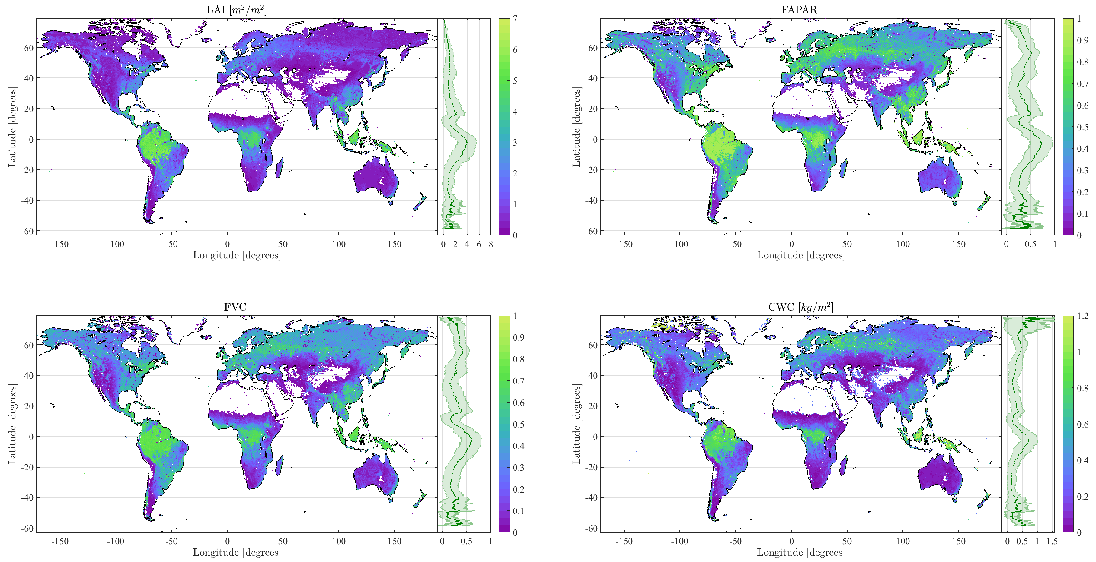
- The development of a general methodology for global LAI/FAPAR estimation including FVC and CWC which are not provided by MODIS.
- The use of a global plant traits database (composed of thousands of data) for probability density function (PDF) estimation with copulas to be used for radiative transfer modeling leaf parameterization.
- The enforceability of biophysical parameter retrieval chain over GEE exploiting its capabilities to provide climate data records of global biophysical variables at computationally both affordable and efficient way.
2. Data Collection
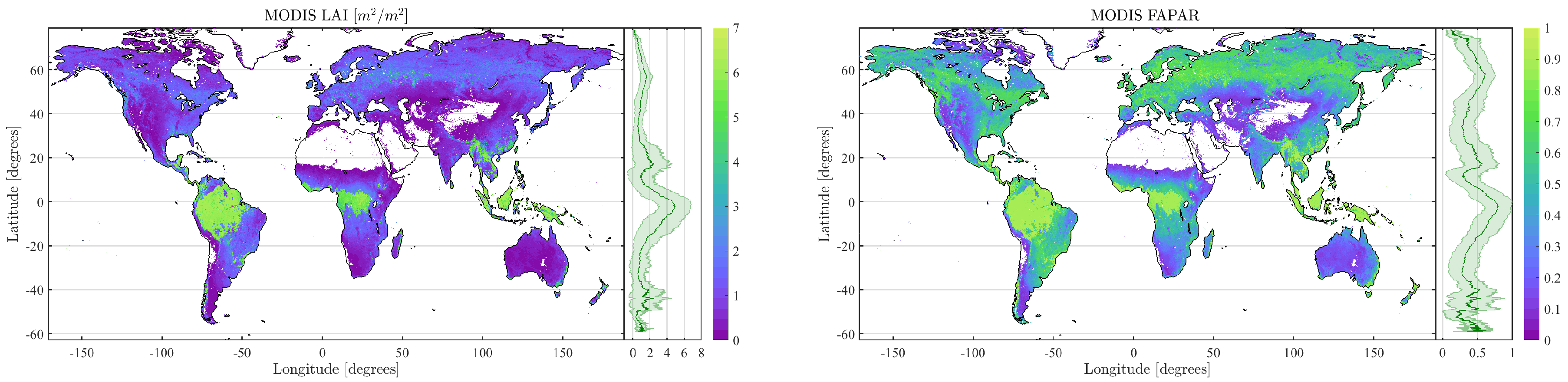
2.1. MODIS Data
2.2. Global Plant Traits
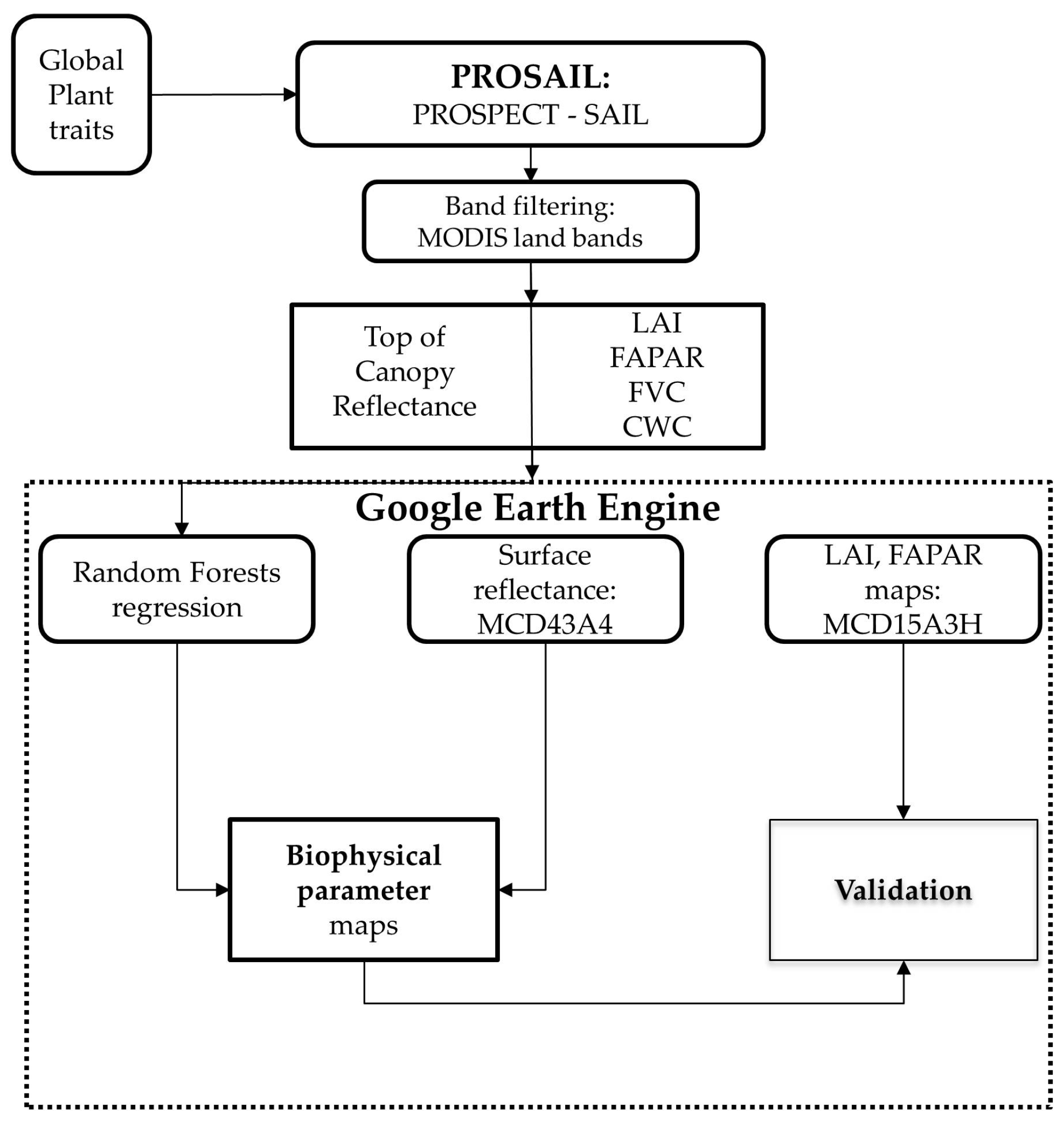
3. Methodology
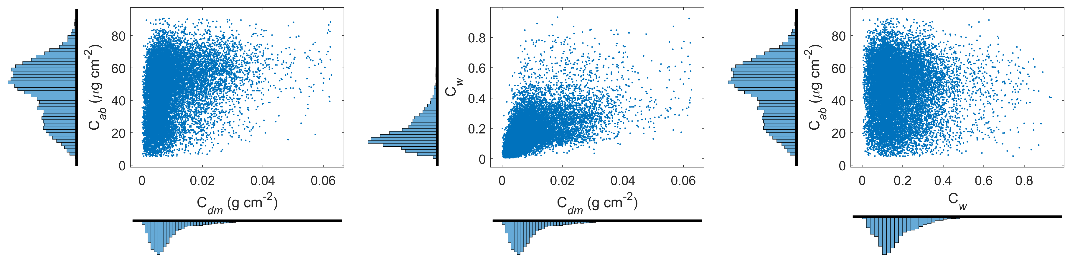
3.1. Creation of Leaf Plant Traits’ Distributions
3.2. Radiative Transfer Modeling
3.3. Random Forests Regression
4. Results and Validation
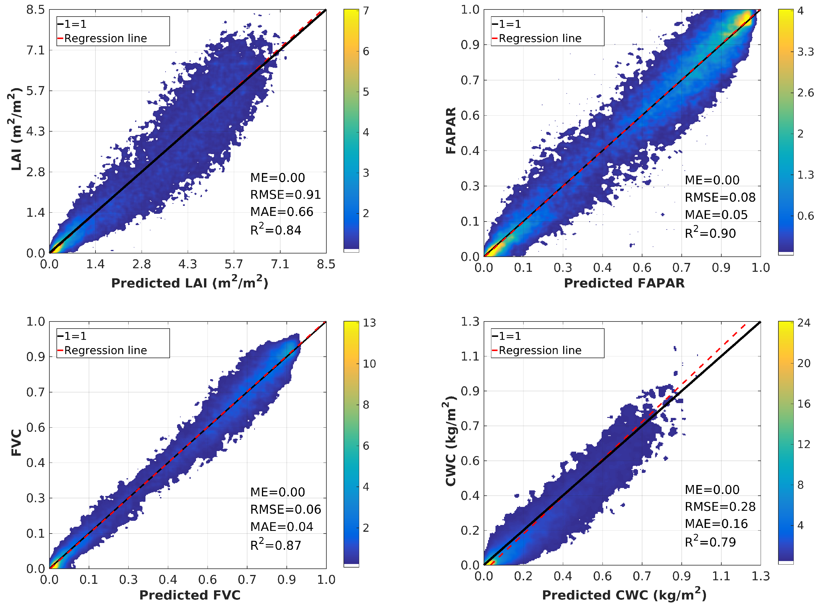
4.1. Random Forests Theoretical Performance
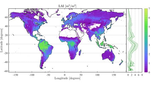
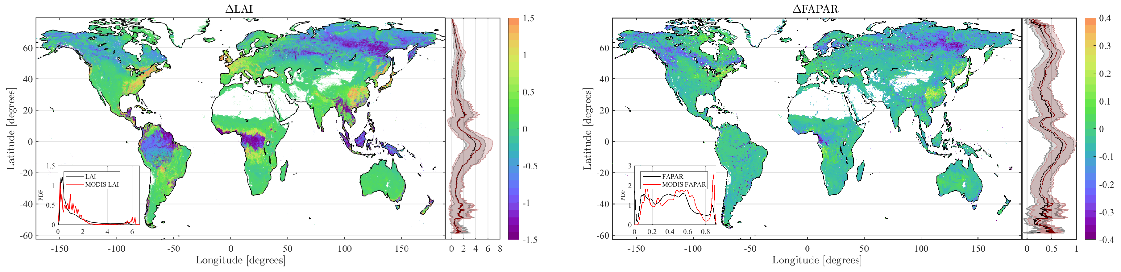
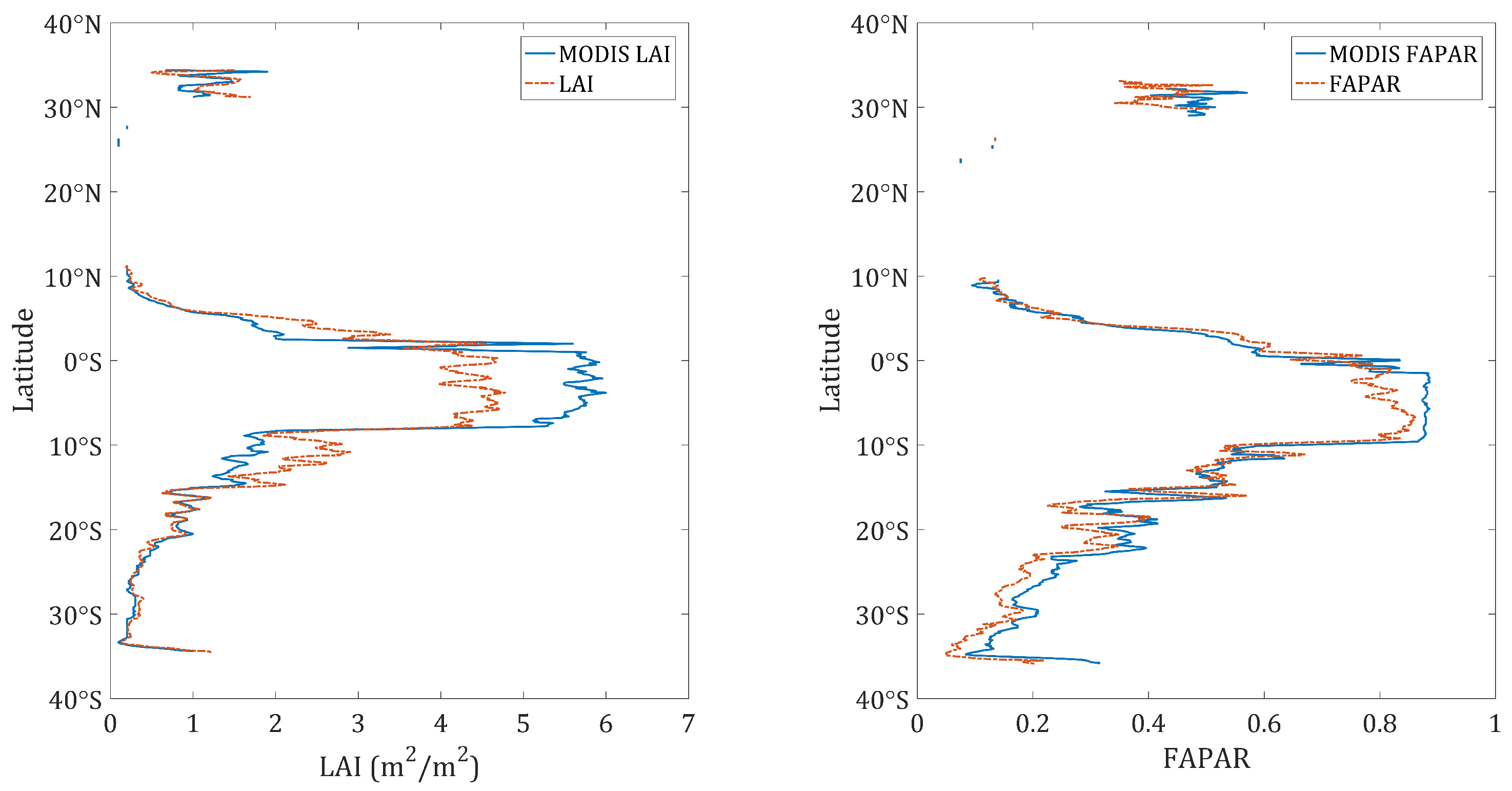
4.2. Obtained Estimates over GEE
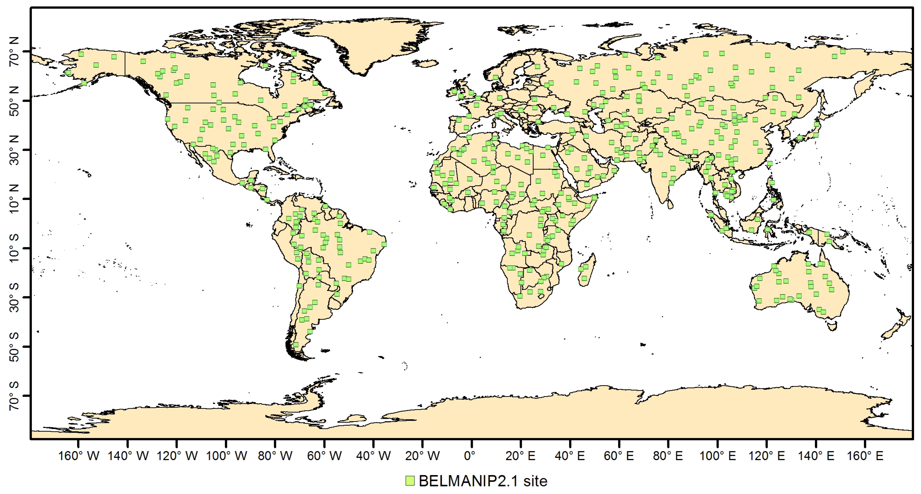
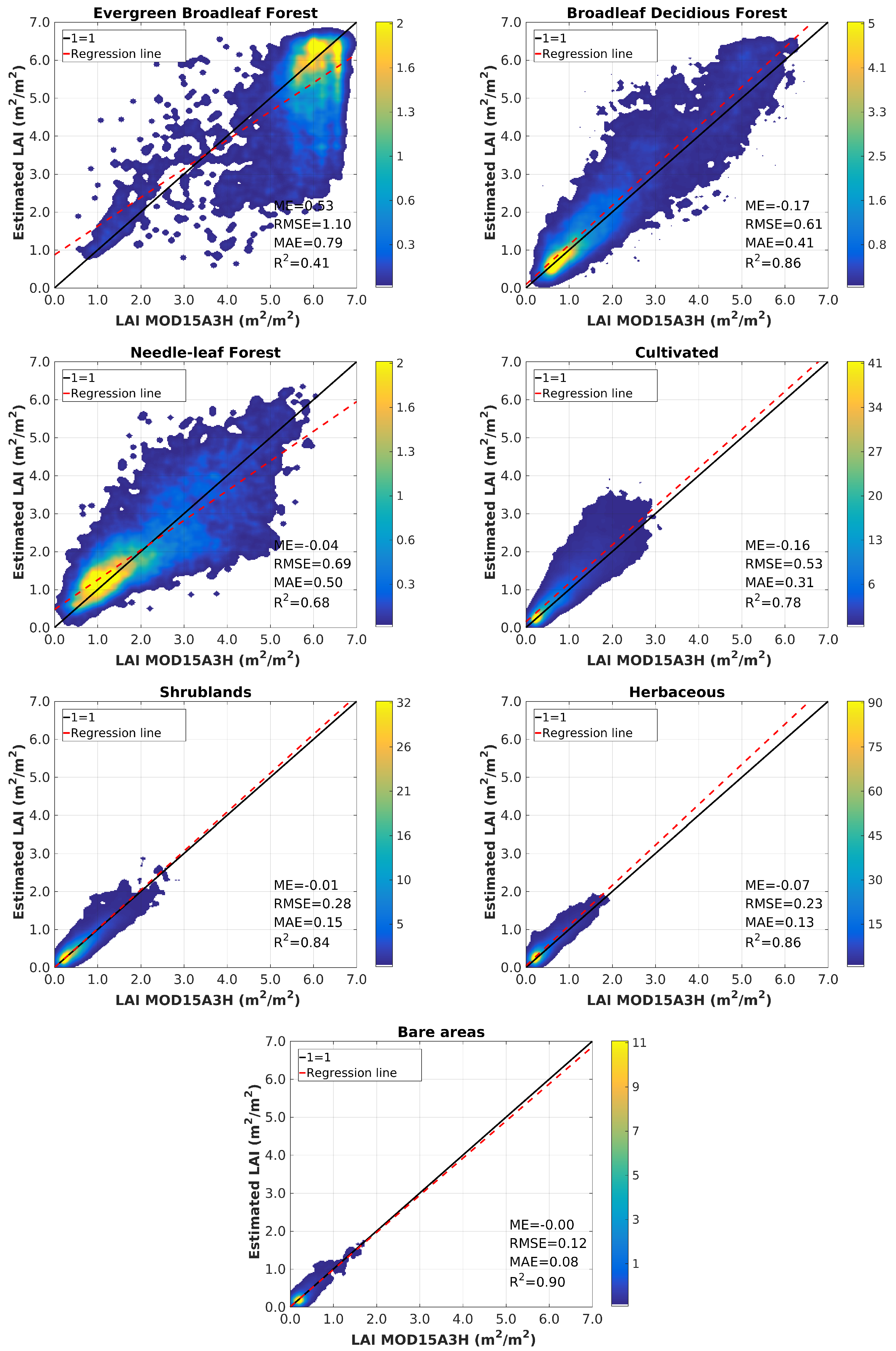
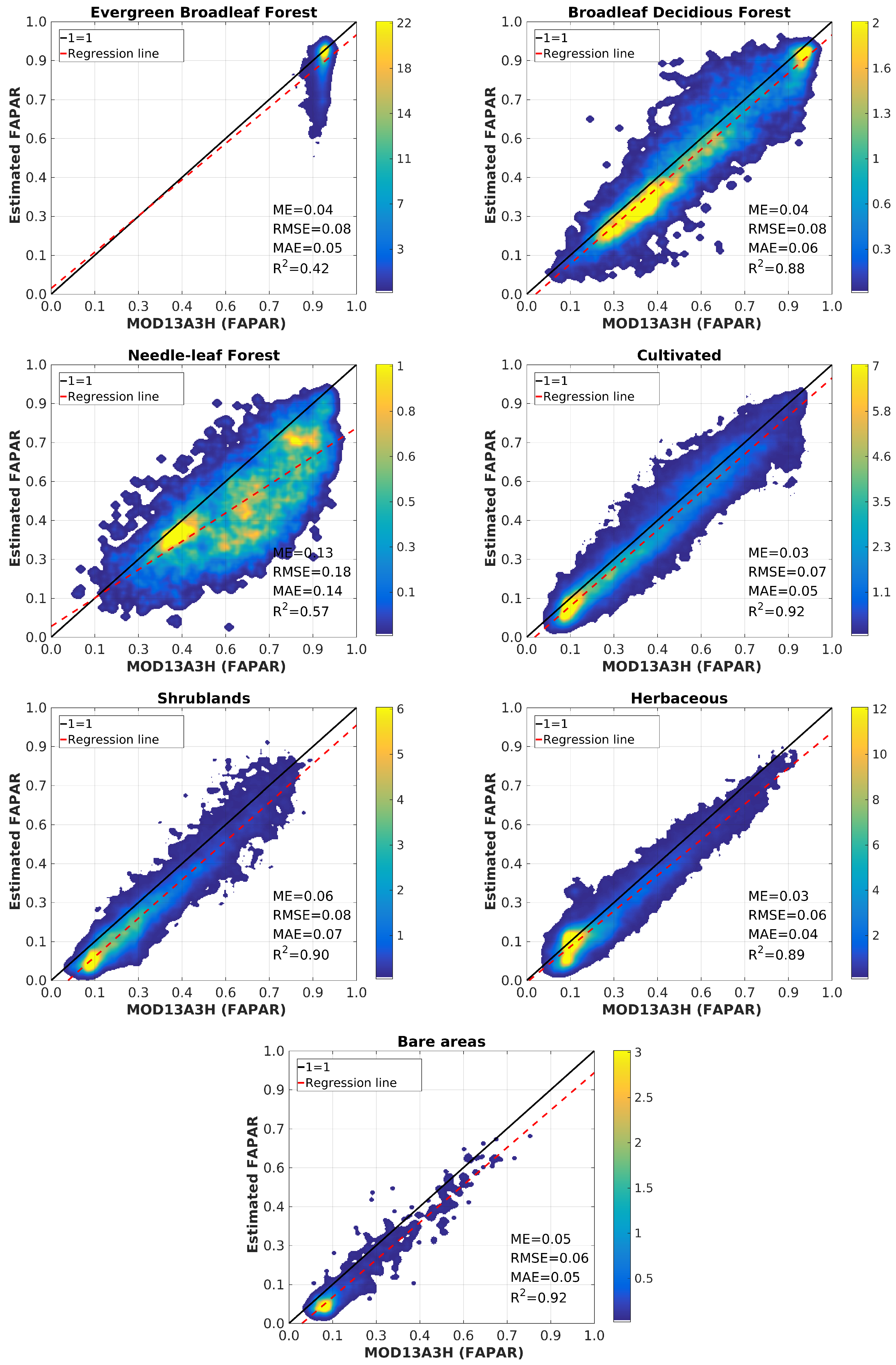
4.3. Validation
5. Discussion
6. Conclusions
Supplementary Materials
Author Contributions
Funding
Acknowledgments
Conflicts of Interest
References
- Raich, J.W.; Schlesinger, W.H. The global carbon dioxide flux in soil respiration and its relationship to vegetation and climate. Tellus B 1992, 44, 81–99. [Google Scholar] [CrossRef]
- Beer, C.; Reichstein, M.; Tomelleri, E.; Ciais, P.; Jung, M.; Carvalhais, N.; Rödenbeck, C.; Arain, M.A.; Baldocchi, D.; Bonan, G.B.; et al. Terrestrial Gross Carbon Dioxide Uptake: Global Distribution and Covariation with Climate. Science 2010, 329, 834–838. [Google Scholar] [CrossRef] [PubMed]
- Huete, A.; Didan, K.; Miura, T.; Rodriguez, E.P.; Gao, X.; Ferreira, L.G. Overview of the radiometric and biophysical performance of the MODIS vegetation indices. Remote Sens. Environ. 2002, 83, 195–213. [Google Scholar] [CrossRef]
- Fensholt, R. Earth observation of vegetation status in the Sahelian and Sudanian West Africa: Comparison of Terra MODIS and NOAA AVHRR satellite data. Int. J. Remote Sens. 2004, 25, 1641–1659. [Google Scholar] [CrossRef]
- Clevers, J.G.P.W.; Kooistra, L.; Schaepman, M.E. Estimating canopy water content using hyperspectral remote sensing data. Int. J. Appl. Earth Obs. Geoinf. 2010, 12, 119–125. [Google Scholar] [CrossRef]
- Yebra, D.P.; Chuvieco, E.; Riaño, D.; Zylstra, P.; Hunt, R.; Danson, F.M.; Qi, Y.; Jurdao, S. A global review of remote sensing of live fuel moisture content for fire danger assessment, moving towards operational products. Remote Sens. Environ. 2013, 136, 455–468. [Google Scholar] [CrossRef]
- Wulder, M. Optical remote-sensing techniques for the assessment of forest inventory and biophysical parameters. Prog. Phys. Geogr. 1998, 22, 449–476. [Google Scholar] [CrossRef]
- Zheng, G.; Monika, M. Retrieving leaf area index (LAI) using remote sensing: theories, methods and sensors. Sensors 1998, 9, 2719–2745. [Google Scholar] [CrossRef] [PubMed]
- Verrelst, J.; Camps-Valls, G.; Muñoz-Marí, J.; Rivera, J.P.; Veroustraete, F.; Clevers, J.G.; Moreno, J. Optical remote sensing and the retrieval of terrestrial vegetation bio-geophysical properties—A review. ISPRS J. Photogramm. Remote Sens. 2015, 108, 273–290. [Google Scholar] [CrossRef]
- Haykin, S. Neural Networks—A Comprehensive Foundation, 2nd ed.; Prentice Hall: Upper Saddle River, NJ, USA, 1999. [Google Scholar]
- Breiman, L. Random forests. Mach. Learn. 2001, 45, 5–32. [Google Scholar] [CrossRef]
- Camps-Valls, G.; Bruzzone, L. Kernel Methods for Remote Sensing Data Analysis; Wiley & Sons: Chichester, UK, 2009; p. 434. ISBN 978-0-470-72211-4. [Google Scholar]
- Myneni, R.B.; Ramakrishna, R.; Nemani, R.; Running, S.W. Estimation of global leaf area index and absorbed PAR using radiative transfer models. IEEE Trans. Geosci. Remote Sens. 1997, 35, 1380–1393. [Google Scholar] [CrossRef]
- Kimes, D.S.; Knyazikhin, Y.; Privette, J.L.; Abuelgasim, A.A.; Gao, F. Inversion methods for physically-based models. Remote Sens. Rev. 2000, 18, 381–439. [Google Scholar] [CrossRef]
- Knyazikhin, Y.; Glassy, J.; Privette, J.L.; Tian, Y.; Lotsch, A.; Zhang, Y.; Wang, Y.; Morisette, J.T.; Votava, P.; Myneni, R.B.; et al. MODIS Leaf Area Index (LAI) and Fraction of Photosynthetically Active Radiation Absorbed by Vegetation (FPAR) Product (MOD15) Algorithm Theoretical Basis Document; NASA Goddard Space Flight Center: Greenbelt, MD, USA, 1999; Volume 20771. [Google Scholar]
- Campos-Taberner, M.; García-Haro, F.J.; Camps-Valls, G.; Grau-Muedra, G.; Nutini, F.; Crema, A.; Boschetti, M. Multitemporal and multiresolution leaf area index retrieval for operational local rice crop monitoring. Remote Sens. Environ. 2016, 187, 102–118. [Google Scholar] [CrossRef]
- Campos-Taberner, M.; García-Haro, F.J.; Camps-Valls, G.; Grau-Muedra, G.; Nutini, F.; Busetto, L.; Katsantonis, D.; Stavrakoudis, D.; Minakou, C.; Gatti, L.; et al. Exploitation of SAR and Optical Sentinel Data to Detect Rice Crop and Estimate Seasonal Dynamics of Leaf Area Index. Remote Sens. 2017, 9, 248. [Google Scholar] [CrossRef]
- Svendsen, D.H.; Martino, L.; Campos-Taberner, M.; García-Haro, F.J.; Camps-Valls, G. Joint Gaussian Processes for Biophysical Parameter Retrieval. IEEE Trans. Geosci. Remote Sens. 2018, 56, 1718–1727. [Google Scholar] [CrossRef]
- Baret, F.; Hagolle, O.; Geiger, B.; Bicheron, P.; Miras, B.; Huc, M.; Berthelot, B.; Niño, F.; Weiss, M.; Samain, O.; et al. LAI, fAPAR and fCover CYCLOPES global products derived from VEGETATION: Part 1: Principles of the algorithm. Remote Sens. Environ. 2007, 110, 275–286. [Google Scholar] [CrossRef]
- Baret, F.; Jacquemoud, S.; Guyot, G.; Leprieur, C. Modeled analysis of the biophysical nature of spectral shifts and comparison with information content of broad bands. Remote Sens. Environ. 1992, 41, 133–142. [Google Scholar] [CrossRef]
- García-Haro, F.J.; Campos-Taberner, M.; Muñoz-Marí, J.; Laparra, V.; Camacho, F.; Sánchez-Zapero, J.; Camps-Valls, G. Derivation of global vegetation biophysical parameters from EUMETSAT Polar System. ISPRS J. Photogramm. Remote Sens. 2018, 139, 57–74. [Google Scholar] [CrossRef]
- Jacquemound, S.; Bidel, L.; Francois, C.; Pavan, G. ANGERS Leaf Optical Properties Database (2003). Data Set. Available online: http://ecosis.org (accessed on 5 June 2018).
- Gitelson, A.A.; Merzlyak, M.N. Remote sensing of chlorophyll concentration in higher plant leaves. Adv. Space Res. 1998, 22, 689–692. [Google Scholar] [CrossRef]
- Gitelson, A.A.; Buschmann, C.; Lichtenthaler, H.K. Leaf chlorophyll fluorescence corrected for re-absorption by means of absorption and reflectance measurements. J. Plant Physiol. 1998, 152, 283–296. [Google Scholar] [CrossRef]
- Hosgood, B.; Jacquemoud, S.; Andreoli, G.; Verdebout, J.; Pedrini, G.; Schmuck, G. Leaf Optical Properties Experiment 93 (LOPEX93); European Commission—Joint Research Centre: Ispra, Italy, 1994; p. 20. Available online: https://data.ecosis.org/dataset/13aef0ce-dd6f-4b35-91d9-28932e506c41/resource/4029b5d3-2b84-46e3-8fd8-c801d86cf6f1/download/leaf-optical-properties-experiment-93-lopex93.pdf (accessed on 5 June 2018).
- Feret, J.B.; François, C.; Asner, G.P.; Gitelson, A.A.; Martin, R.E.; Bidel, L.P.R.; Ustin, S.L.; Le Maire, G.; Jacquemoud, S. PROSPECT-4 and 5: Advances in the leaf optical properties model separating photosynthetic pigments. Remote Sens. Environ. 2008, 112, 3030–3043. [Google Scholar] [CrossRef]
- Combal, B.; Baret, F.; Weiss, M.; Trubuil, A.; Mace, D.; Pragnere, A.; Myneni, R.B.; Knyazikhin, Y.; Wang, L. Retrieval of canopy biophysical variables from bidirectional reflectance using prior information to solve the ill-posed inverse problem. Remote Sens. Environ. 2002, 84, 1–15. [Google Scholar] [CrossRef]
- Kattge, J.; Díaz, S.; Lavorel, S.; Prentice, I.C.; Leadley, P.; Bönisch, G.; Garnier, E.; Westoby, M.; Reich, P.B.; Wright, I.J.; et al. TRY—A global database of plant traits. Glob. Chang. Biol. 2011, 17, 2905–2935. [Google Scholar] [CrossRef]
- Wulder, M.A.; Coops, N.C. Make Earth observations open access: Freely available satellite imagery will improve science and environmental-monitoring products. Nature 2014, 513, 30–32. [Google Scholar] [CrossRef] [PubMed]
- Gorelick, N.; Hancher, M.; Dixon, M.; Ilyushchenko, S.; Thau, D.; Moore, R. Google Earth Engine: Planetary-scale geospatial analysis for everyone. Remote Sens. Environ. 2017, 202, 18–27. [Google Scholar] [CrossRef]
- Robinson, N.P.; Allread, B.W.; Jones, M.O.; Moreno, A.; Kimball, J.S.; Naugle, D.E.; Erickson, T.A.; Richardson, A.D. A dynamic Landsat derived Normalized Difference Vegetation Index (NDVI) product for the Conterminous United States. Remote Sens. 2017, 9, 863. [Google Scholar] [CrossRef]
- Attermeyer, K.; Flury, S.; Jayakumar, R.; Fiener, P.; Steger, K.; Arya, V.; Wilken, F.; Van Geldern, R.; Premke, K. Invasive floating macrophytes reduce greenhouse gas emissions from a small tropical lake. Sci. Rep. 2016, 6, 20424. [Google Scholar] [CrossRef] [PubMed]
- Yu, M.; Gao, Q.; Gao, C.; Wang, C. Extent of night warming and spatially heterogeneous cloudiness differentiate temporal trend of greenness in mountainous tropics in the new century. Sci. Rep. 2017, 7, 41256. [Google Scholar] [CrossRef] [PubMed]
- He, M.; Kimball, J.S.; Maneta, M.P.; Maxwell, B.D.; Moreno, A.; Begueria, S.; Wu, X. Regional Crop Gross Primary Productivity and Yield Estimation Using Fused Landsat-MODIS Data. Remote Sens. 2018, 10, 372. [Google Scholar] [CrossRef]
- Kraaijenbrink, P.D.A.; Bierkens, M.F.P.; Lutz, A.F.; Immerzeel, W.W. Impact of a global temperature rise of 1.5 degrees Celsius on Asia’s glaciers. Nature 2017, 549, 257–260. [Google Scholar] [CrossRef] [PubMed]
- Reichstein, M.; Bahn, M.; Mahecha, M.D.; Kattge, J.; Baldocchi, D.D. Linking plant and ecosystem functional biogeography. Proc. Natl. Acad. Sci. USA 2014, 111, 13697–13702. [Google Scholar] [CrossRef] [PubMed]
- Van Bodegom, P.M.; Douma, J.C.; Verheijen, L.M. A fully traits-based approach to modeling global vegetation distribution. Proc. Natl. Acad. Sci. USA 2014, 111, 13733–13738. [Google Scholar] [CrossRef] [PubMed]
- Madani, N.; Kimball, J.S.; Ballantyne, A.P.; Affleck, D.L.R.; Bodegom, P.M.; Reich, P.B.; Kattge, J.; Sala, A.; Nazeri, M.; Jones, M.; et al. Future global productivity will be affected by plant trait response to climate. Sci. Rep. 2018, 8, 2870. [Google Scholar] [CrossRef] [PubMed]
- Wirth, C.; Lichstein, J.W. The Imprint of Species Turnover on Old-Growth Forest Carbon Balances-Insights From a Trait-Based Model of Forest Dynamics. In Old-Growth Forests; Wirth, C., Heimann, M., Gleixner, G., Eds.; Springer: Jena, Germany, 2009; pp. 81–113. ISBN 978-3-540-92705-1. [Google Scholar]
- Ziehn, T.; Kattge, J.; Knorr, W.; Scholze, M. Improving the predictability of global CO2 assimilation rates under climate change. Geophys. Res. Lett. 2011, 38, 10. [Google Scholar] [CrossRef]
- Berger, K.; Atzberger, C.; Danner, M.; D’Urso, G.; Mauser, W.; Vuolo, F.; Hank, T. Evaluation of the PROSAIL Model Capabilities for Future Hyperspectral Model Environments: A Review Study. Remote Sens. 2018, 10, 85. [Google Scholar] [CrossRef]
- Bacour, C.; Baret, F.; Béal, D.; Weiss, M.; Pavageau, K. Neural network estimation of LAI, fAPAR, fCover and LAIxCab, from top of canopy MERIS reflectance data: Principles and validation. Remote Sens. Environ. 2014, 105, 313–325. [Google Scholar] [CrossRef]
- Si, Y.; Schlerf, M.; Zurita-Milla, R.; Skidmore, A.; Wang, T. Mapping spatio-temporal variation of grassland quantity and quality using MERIS data and the PROSAIL model. Remote Sens. Environ. 2012, 121, 415–425. [Google Scholar] [CrossRef]
- Friedl, M.A.; Sulla-Menashe, D.; Tan, B.; Schneider, A.; Ramankutty, N.; Sibley, A.; Huang, X. MODIS Collection 5 global land cover: Algorithm refinements and characterization of new datasets. Remote Sens. Environ. 2010, 114, 168–182. [Google Scholar] [CrossRef]
- Parzen, E. On estimation of a probability density function and mode. Ann. Math. Stat. 1962, 33, 1065–1076. [Google Scholar] [CrossRef]
- Reich, P.B. The world-wide ‘fast–slow’ plant economics spectrum: A traits manifesto. J. Ecol. 2014, 102, 275–301. [Google Scholar] [CrossRef]
- Nelsen, R.B. An Introduction to Copulass, 2nd ed.; Springer Science & Business Media: New York, NY, USA, 2009; ISBN 978-0387-28659-4. [Google Scholar]
- Žežula, I. On multivariate Gaussian copulas. J. Stat. Plan. Inference 2009, 111, 3942–3946. [Google Scholar] [CrossRef]
- Jacquemoud, S.; Baret, F. PROSPECT: A model of leaf optical properties spectra. Remote Sens. Environ. 1990, 34, 75–191. [Google Scholar] [CrossRef]
- Verhoef, W. Light scattering by leaf layers with application to canopy reflectance modeling: The SAIL model. Remote Sens. Environ. 1984, 16, 125–141. [Google Scholar] [CrossRef]
- Breiman, L.; Friedman, J.H. Estimating Optimal Transformations for Multiple Regression and Correlation. J. Am. Stat. Assoc. 1985, 391, 1580–1598. [Google Scholar]
- Evans, J.S.; Cushman, S.A. Gradient modeling of conifer species using random forests. Landsc. Ecol. 2009, 24, 673–683. [Google Scholar] [CrossRef]
- Oliveira, S.; Oehler, F.; San-Miguel-Ayanz, J.; Camia, A.; Pereira, J.M.C. Modeling spatial patterns of fire occurrence in Mediterranean Europe using Multiple Regression and Random Forest. For. Ecol. Manag. 2012, 275, 117–129. [Google Scholar] [CrossRef]
- Gislason, P.O.; Benediktsson, J.A.; Sveinsson, J.R. Random Forests for land cover classification. Pattern Recognit. Lett. 2006, 27, 294–300. [Google Scholar] [CrossRef]
- Cutler, D.R.; Edwards, T.C.; Beard, K.H.; Cutler, A.; Hess, K.T.; Gibson, J.; Lawler, J.J. Random Forests for classification in ecology. Ecology 2007, 88, 2783–2792. [Google Scholar] [CrossRef] [PubMed]
- Genuer, R.; Poggi, J.M.; Tuleau-Malot, C. Variable selection using random forests. Pattern Recognit. Lett. 2010, 31, 2225–2236. [Google Scholar] [CrossRef]
- Jung, M.; Zscheischler, J. A Guided Hybrid Genetic Algorithm for Feature Selection with Expensive Cost Functions. Procedia Comput. Sci. 2013, 18, 2337–2346. [Google Scholar] [CrossRef]
- Baret, F.; Morissette, J.T.; Fernandes, R.; Champeaux, J.L.; Myneni, R.B.; Chen, J.; Plummer, S.; Weiss, M.; Bacour, C.; Garrigues, S.; et al. Evaluation of the representativeness of networks of sites for the global validation and intercomparison of land biophysical products: proposition of the CEOS-BELMANIP. IEEE Trans. Geosci. Remote Sens. 2006, 44, 1794–1803. [Google Scholar] [CrossRef]
- Yan, K.; Park, T.; Yan, G.; Liu, Z.; Yang, B.; Chen, C.; Nemani, R.R.; Knyazikhin, Y.; Myneni, R.B. Evaluation of MODIS LAI/FPAR Product Collection 6. Part 2: Validation and Intercomparison. Remote Sens. 2016, 8, 460. [Google Scholar] [CrossRef]
- Camacho, F.; Cernicharo, J.; Lacaze, R.; Baret, F.; Weiss, M. GEOV1: LAI, FAPAR essential climate variables and FCOVER global time series capitalizing over existing products. Part 2: Validation and intercomparison with reference products. Remote Sens. Environ. 2013, 137, 310–329. [Google Scholar] [CrossRef]
- Nestola, E.; Sánchez-Zapero, J.; Latorre, C.; Mazzenga, F.; Matteucci, G.; Calfapietra, C.; Camacho, F. Validation of PROBA-V GEOV1 and MODIS C5 & C6 fAPAR Products in a Deciduous Beech Forest Site in Italy. Remote Sens. 2017, 9, 126. [Google Scholar]
- Baret, F.; Weiss, M.; Lacaze, R.; Camacho, F.; Makhmara, H.; Pacholcyzk, P.; Smets, B. GEOV1: LAI and FAPAR essential climate variables and FCOVER global time series capitalizing over existing products. Part 1: Principles of development and production. Remote Sens. Environ. 2013, 137, 299–309. [Google Scholar] [CrossRef]
- Campos-Taberner, M.; García-Haro, F.J.; Busetto, L.; Ranghetti, L.; Martínez, B.; Gilabert, M.A.; Camps-Valls, G.; Camacho, F.; Boschetti, M. A Critical Comparison of Remote Sensing Leaf Area Index Estimates over Rice-Cultivated Areas: From Sentinel-2 and Landsat-7/8 to MODIS, GEOV1 and EUMETSAT Polar System. Remote Sens. 2018, 10, 763. [Google Scholar] [CrossRef]
- Xu, B.; Park, T.; Yan, K.; Chen, C.; Zeng, Y.; Song, W.; Yin, G.; Li, J.; Liu, Q.; Knyazikhin, Y.; et al. Analysis of Global LAI/FPAR Products from VIIRS and MODIS Sensors for Spatio-Temporal Consistency and Uncertainty from 2012–2016. Forests 2018, 9, 73. [Google Scholar] [CrossRef]


| MCD43A4 Band | Wavelength (nm) |
|---|---|
| Band 1 (red) | 620–670 |
| Band 2 (NIR) | 841–876 |
| Band 3 (blue) | 459–479 |
| Band 4 (green) | 545–565 |
| Band 5 (SWIR-1) | 1230–1250 |
| Band 6 (SWIR-2) | 1628–1652 |
| Band 7 (MWIR) | 2105–2155 |
| Trait Name | Number of Samples | Number of Species |
|---|---|---|
| C | 19,222 | 941 |
| C | 69,783 | 11,908 |
| C | 32,020 | 4802 |
| Parameter | Min | Max | Mode | Std | Type | |
|---|---|---|---|---|---|---|
| Leaf | N | 1.2 | 2.2 | 1.6 | 0.3 | Gaussian |
| C (g·cm) | - | - | - | - | KDE * | |
| C (g·cm) | 0.6 | 16 | 5 | 7 | Gaussian | |
| C (g·cm) | - | - | - | - | KDE * | |
| C | - | - | - | - | KDE * | |
| C | 0 | 0 | 0 | 0 | - | |
| Canopy | LAI (m/m) | 0 | 8 | 3.5 | 4 | Gaussian |
| ALA (°) | 35 | 80 | 60 | 12 | Gaussian | |
| Hotspot | 0.1 | 0.5 | 0.2 | 0.2 | Gaussian | |
| vCover | 0.3 | 1 | 0.99 | 0.2 | Truncated Gaussian | |
| Soil | 0.1 | 1 | 0.8 | 0.6 | Gaussian | |
© 2018 by the authors. Licensee MDPI, Basel, Switzerland. This article is an open access article distributed under the terms and conditions of the Creative Commons Attribution (CC BY) license (http://creativecommons.org/licenses/by/4.0/).
Share and Cite
Campos-Taberner, M.; Moreno-Martínez, Á.; García-Haro, F.J.; Camps-Valls, G.; Robinson, N.P.; Kattge, J.; Running, S.W. Global Estimation of Biophysical Variables from Google Earth Engine Platform. Remote Sens. 2018, 10, 1167. https://doi.org/10.3390/rs10081167
Campos-Taberner M, Moreno-Martínez Á, García-Haro FJ, Camps-Valls G, Robinson NP, Kattge J, Running SW. Global Estimation of Biophysical Variables from Google Earth Engine Platform. Remote Sensing. 2018; 10(8):1167. https://doi.org/10.3390/rs10081167
Chicago/Turabian StyleCampos-Taberner, Manuel, Álvaro Moreno-Martínez, Francisco Javier García-Haro, Gustau Camps-Valls, Nathaniel P. Robinson, Jens Kattge, and Steven W. Running. 2018. "Global Estimation of Biophysical Variables from Google Earth Engine Platform" Remote Sensing 10, no. 8: 1167. https://doi.org/10.3390/rs10081167
APA StyleCampos-Taberner, M., Moreno-Martínez, Á., García-Haro, F. J., Camps-Valls, G., Robinson, N. P., Kattge, J., & Running, S. W. (2018). Global Estimation of Biophysical Variables from Google Earth Engine Platform. Remote Sensing, 10(8), 1167. https://doi.org/10.3390/rs10081167