Article

Validation of the EGSIEM GRACE Gravity Fields Using GNSS Coordinate Timeseries and In-Situ Ocean Bottom Pressure Records

1
Geophysics Laboratory, Faculty of Science, Technology and Communication, University of Luxembourg, 4365 Luxembourg, Luxembourg
2
GFZ German Research Centre for Geosciences, 14473 Potsdam, Germany
3
Institute of Geodesy, Leibniz University of Hannover, 30167 Hannover, Germany
*
Authors to whom correspondence should be addressed.
Remote Sens. 2018, 10(12), 1976; https://doi.org/10.3390/rs10121976
Submission received: 25 September 2018 / Revised: 28 November 2018 / Accepted: 5 December 2018 / Published: 7 December 2018
(This article belongs to the Special Issue GRACE Facing the Challenge of Extreme Spatial and Temporal Scales)

Abstract

:
Over the 15 years of the Gravity Recovery and Climate Experiment (GRACE) mission, various data processing approaches were developed to derive time-series of global gravity fields based on sensor observations acquired from the two spacecrafts. In this paper, we compare GRACE-based mass anomalies provided by various processing groups against Global Navigation Satellite System (GNSS) station coordinate time-series and in-situ observations of ocean bottom pressure. In addition to the conventional GRACE-based global geopotential models from the main processing centers, we focus particularly on combined gravity field solutions generated within the Horizon2020 project European Gravity Service for Improved Emergency Management (EGSIEM). Although two validation techniques are fully independent from each other, it is demonstrated that they confirm each other to a large extent. Through the validation, we show that the EGSIEM combined long-term monthly solutions are comparable to CSR RL05 and ITSG2016, and better than the other three considered GRACE monthly solutions AIUB RL02, GFZ RL05a, and JPL RL05.1. Depending on the GNSS products, up to 25.6% mean Weighted Root-Mean-Square (WRMS) reduction is obtained when comparing GRACE to the ITRF2014 residuals over 236 GNSS stations. In addition, we also observe remarkable agreement at the annual period between GNSS and GRACE with up to 73% median WRMS reduction when comparing GRACE to the 312 EGSIEM-reprocessed GNSS time series. While the correspondence between GRACE and ocean bottom pressure data is overall much smaller due to lower signal to noise ratio over the oceans than over the continents, up to 50% agreement is found between them in some regions. The results fully confirm the conclusions found using GNSS.

Graphical Abstract

1. Introduction

During the 15 years of the Gravity Recovery and Climate Experiment (GRACE) mission [1], a number of GRACE data processing approaches have been developed and greatly advanced to derive global geopotential models (GGMs) from the raw sensor data observed by the twin GRACE satellites. For the majority of those approaches, different releases exist thanks to successive refinements of the methodology, re-processed Level-1 sensor data, or improved geophysical background models. In addition, a number of post-processing options were developed over the years that are necessary to transform gravity fields into global surface mass estimates. For geophysical applications of the GRACE results, it is important to obtain independent evidence about the quality of different GRACE products and their associated error estimates by means of independent validation.
Within the European Gravity Service for Improved Emergency Management (EGSIEM) [2] project funded by the European Union (EU) under the Horizon2020 program, various GRACE gravity products have been generated including Level-2 monthly gravity solutions from individual Analysis Centers (ACs), combined monthly gravity solutions at both solution level [3] and normal equation level [4], Level-3 gravity products, post-processed daily gravity fields, and near real time (NRT) daily gravity solutions. Validation of the gravity products has been an essential part in the EGSIEM project as validation allows us to assess the quality of our products but also increases user’s confidence in the datasets produced by EGSIEM. To evaluate the quality of different gravity field solutions, two types of external datasets, i.e., GNSS time series and in-situ ocean bottom pressure (OBP) measurements, have been used.
Comparisons of GNSS and GRACE has been undertaken since the first GRACE data releases [5]. With the improvement of both GNSS time series and GRACE gravity products, better agreement has been demonstrated by many other studies at both global [6,7,8,9,10] and regional scale [11,12]. For example, the very recent study by Gu et al. (2017) [9] has compared vertical displacements of 105 globally distributed stations from GPS and GRACE using multi-institution solutions and demonstrated a mean WRMS reduction up to 15% using the ITSG2016 GRACE products and the GNSS products from the IGS (International GNSS Service) analysis center JPL. In addition, Chanard et al. (2018) [10] compared both vertical and horizontal deformation from ITRF 2014 GNSS time series and GRGS RL03 GRACE products and obtained an adjusted mean WRMS reduction up to 14.7% in the vertical component. In our validation work, we mainly use the vertical displacements from both techniques, which show stronger signals than the horizontal component.
In addition to the contribution of the GRACE data to observe land mass changes, GRACE serves as a valuable tool to monitor the oceanic mass variations as well [13]. Local in-situ OBP records have been used to validate the GRACE-derived oceanic mass changes [14,15]. In-situ OBP data have also been used for validation of the new releases of the Atmosphere and Ocean De-aliasing Level 1B (AOD1B) product [16,17], as well as for the validation of ocean model simulations and monthly GRACE gravity fields [18].
In this paper, we compare many different GRACE gravity products with GNSS vertical time series and in-situ OBP measurements in an attempt to gauge the relative quality of the GRACE solutions. We must assume that the GNSS and OBP observations represent the true surface displacement or mass signal. However, it is well known that GNSS position observations contain errors at periodic frequencies in particular the draconitic year signal [19,20]. We cannot estimate the magnitude of these errors. The reader should bear this limitation in mind when interpreting the results presented here.
In Section 2 we present the basic concept of validation, and we introduce the metrics we use to evaluate the quality of the comparisons between GRACE and GNSS or OBP. In Section 3 we describe the datasets used for validation in this paper. Section 4 and Section 5 present the validation results from GNSS time series and the OBP records, respectively. We discuss briefly our validation results in Section 6 and the conclusions are summarized in Section 7.

2. Methodology

2.1. Concept of Validation

Temporal variations in the distribution of mass in or on the Earth cause the Earth’s surface to subside or rebound and are observed in GNSS coordinate solutions e.g., [21,22]. Through the elastic loading theory [23], we can use the surface mass variations, which are observed independently by GRACE in terms of the gravity products represented by spherical harmonic coefficients, to predict surface vertical displacements Δ h at any GNSS station P with a colatitude θ P and longitude λ P using Equation (1) [6,24]
Δ h ( θ P , λ P ) = R n = 1 h n 1 + k n m = 0 n P ¯ n m ( cos θ P ) ( Δ C ¯ n m cos m λ P + Δ S ¯ n m sin m λ P ) ,
where R is the radius of the Earth, h n and k n represent the loading Love numbers [23]. P ¯ n m denotes the normalized associated Legendre functions, and Δ C ¯ n m , Δ S ¯ n m indicate the normalized spherical harmonic coefficients from the GRACE gravity products after removing a long-term mean field. Consequently, GRACE-derived displacements can be compared with GNSS-observed deformation [5,6]. A global network of GNSS stations is used in our validation.
Ocean bottom pressure recorders measure the combined oceanic and atmospheric mass above the sensor. They are therefore directly comparable with time-variable gravity fields and thus suitable for their validation. The validation against in-situ OBP time series is performed using gridded GRACE data. The GRACE equivalent water height data is converted to ocean bottom pressure by:
p ( θ P , λ P ) = ρ g h ( θ P , λ P ) ,
where ρ is the density of sea water, g denotes the mean gravitational acceleration, and h is the equivalent water height.
Using Equations (1) and (2), surface displacements or OBP variations at any GNSS station or in-situ OBP station can be computed from the GRACE gravity spherical harmonics or gridded GRACE gravity products. Subsequently, comparisons of them with the GNSS time series from Section 3.2 and in-situ OBP measurements from Section 3.3 are implemented.

2.2. Metrics for Performance Evaluation
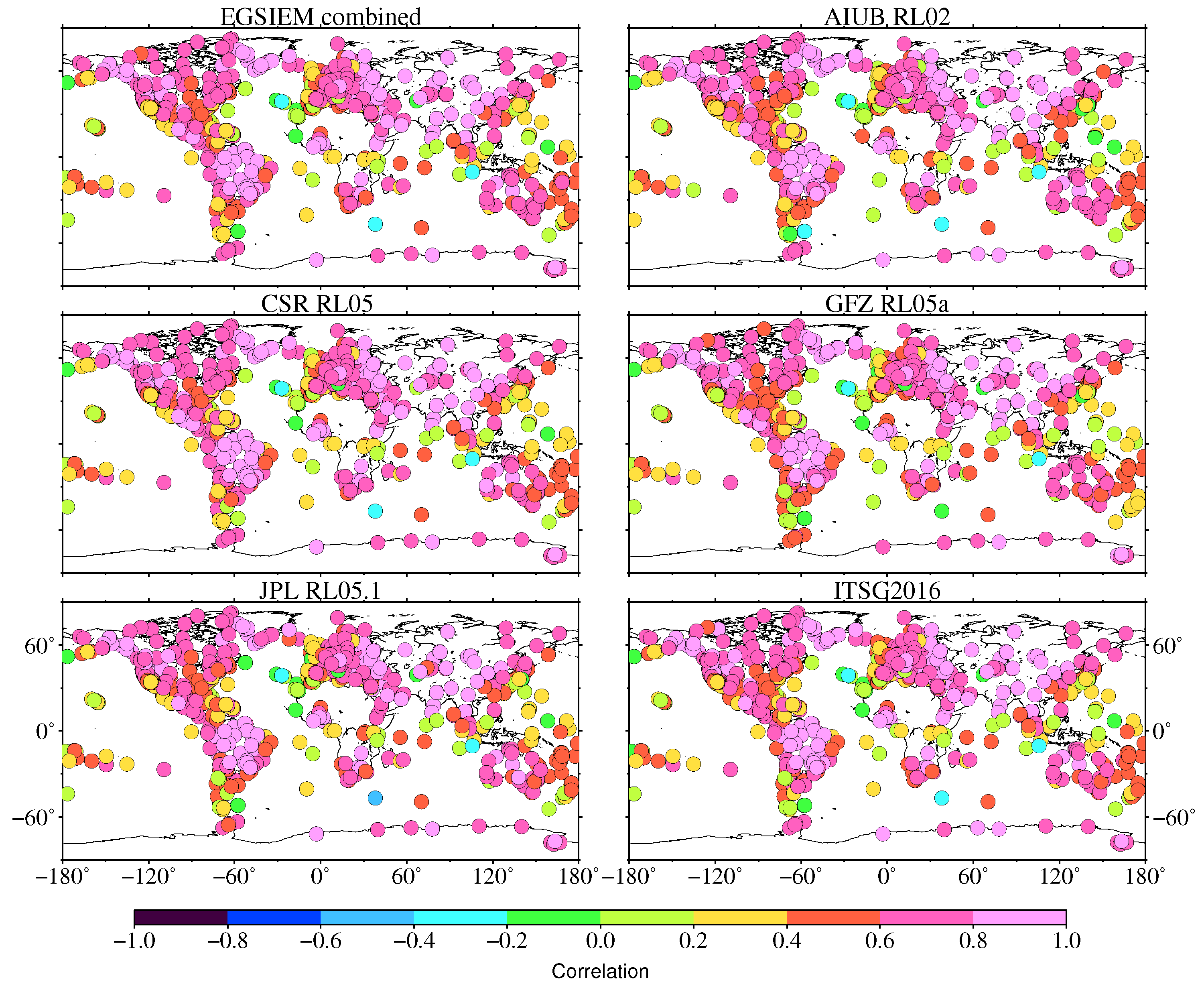
2.2.1. Correlation

The correlation between two time series is a measure of their similarity. However, the correlation coefficient is only sensitive to the phases of two time series but insensitive to any amplitude differences. This characteristic normally leads us to apply further evaluation criteria along with the correlation coefficient.

2.2.2. WRMS Reduction and Its Variants

van Dam et al. (2007) [6] evaluated the similarity between GRACE and GPS for GPS stations in Europe and they measured the WRMS reduction on the GPS vertical surface displacement signal after GRACE predicted surface displacements were removed. The weights of GPS observations were used in this case. Here we use degree and cumulative degree WRMS reduction measures (Equation (3)) which are variants of the WRMS reduction from van Dam et al. (2007) [6]. The traditional WRMS reduction corresponds to the cumulative degree WRMS reduction up to the maximum degree n, i.e., full spectrum. The benefit of using the degree and cumulative degree WRMS reduction analysis is that we are able to evaluate the relative quality of each GRACE gravity field at each spherical harmonic degree.
We use three indicators to assess the quality of gravity field solutions: (1) Mean/median degree WRMS reductions, (2) mean/median cumulative degree WRMS reductions, and (3) WRMS reductions of the time series. The mean/median degree WRMS reduction measures the performance of the gravity solutions at each spherical harmonic degree. A higher degree reduction indicates a better performance. Similarly, the cumulative degree WRMS reduction assesses the performance of the gravity solutions up to the spherical harmonic degree n. The WRMS reduction of the time series corresponds to the traditional WRMS reduction as used by van Dam et al. (2007) [6].
d e g r e e WRMS reduction = WRMS h GPS WRMS h GPS h GRACE n WRMS h GPS .

2.2.3. Standard Deviation Reduction

Similarly, the agreement of the GRACE solutions converted to pressure with the in-situ ocean bottom pressure measurements is expressed in terms of reduction of standard deviation in the in-situ timeseries after GRACE measured data has been removed from them:
STD reduction = STD p in-situ STD p in-situ p GRACE STD p in-situ .
The STD reduction is negative in the case where GRACE increases the variability. It is zero in the case where GRACE does not alter the variance of the in-situ data, and is 100% in the case where GRACE perfectly coincides with the signals observed in-situ. In view of the area-averaging properties of GRACE, an achievement of 100% is highly unlikely.
In essence, the STD reduction is equivalent to the WRMS reduction except that a weight is applied in Equation (3). The error information from the GNSS time series are used as weights [6,10].

3. Datasets

3.1. GRACE Gravity Products

Within the EGSIEM project, combinations of monthly GRACE products were undertaken at both the solution level and the normal equation level. In this study, we use the EGSIEM combined long-term monthly gravity solutions from Jean et al. (2018) [3] who combined the existing monthly GRACE gravity solutions spanning from August 2002 to October 2014. Note that ITSG2014 [25] from TU Graz was combined instead of ITSG2016 [26] at the time of combining all existing monthly solutions. For more detail regarding the EGSIEM combined long-term monthly gravity solutions, the reader is referred to Jean et al. (2018) [3].
In addition to the EGSIEM combined long-term gravity solutions, monthly gravity solutions from the three official GRACE data processing centers, i.e., CSR RL05 [27], GFZ RL05a [28], and JPL RL05.1 [29], as well as other institutions, e.g., AIUB RL02 [30] from UBERN and ITSG2016 [26] from TU Graz, have been included as well. For the comparison with GNSS, all six GRACE L2 GSM (Geopotential coefficients of GRACE-derived static gravity field) spherical harmonic coefficients (SHCs) from both EGSIEM combined and other institutions have been post-processed in the same way. First, the C20 terms, which are poorly observed by GRACE, are replaced with those from SLR produced by Cheng et al. (2013) [31]. Degree-1 coefficients which are missing in the delivered GRACE GSM products are restored by using the datasets provided by Swenson et al. (2008) [32] to be consistent with GNSS in the same CF (Center of Figure) reference frame [33]. The dealiasing products, i.e., GAC products [16], have also been restored to GSM SHCs. Due to the fact that the GRACE-derived SHCs are noisy in nature [1,5], all GSM SHCs are filtered with the Gaussian filter [24,34] with the smoothing radius of 500 km [12]. A long-term mean field of each GRACE gravity product is calculated using its whole time span gravity data and removed from its monthly solutions. Finally, these GSM SHCs are converted into vertical displacements at the selected GNSS stations using Equation (1). The linear trend is removed from each vertical displacement time series in order to remove the GIA effects as well as other tectonic signals [6].
For the comparison with the in-situ OBP measurements, all GRACE solutions have been post-processed in the same manner as used in Poropat et al. [18]: Degree-1 coefficients are approximated according to Bergmann-Wolf et al. [35], C20 is replaced with solutions from Cheng et al. (2013) [31], glacial isostatic adjustment correction is applied based on the model by Paulson et al (2007) [36], co- and post-seismic deformations of the largest earthquakes are estimated and subtracted [37], and the non-isotropic DDK-1 filter [38] is applied. The spherical harmonic coefficients are converted to a 1° grid and GAD [16] is added back to include all the atmospheric and oceanic contributions to the ocean bottom pressure anomalies that were previously removed during de-aliasing. Finally, to align the signal content between GRACE and the pre-processed in-situ OBP data, a trend calculated over the same period is removed from all GRACE solutions.

3.2. GNSS Time Series

To validate the EGSIEM combined monthly GRACE solutions, three different GNSS time series products are used. A global network of GNSS stations have been reprocessed within the EGSIEM project [39] to generate reference frame products spanning from 2003 to 2014. A series of post-processing steps have been applied to the raw GNSS time series, which includes: (1) Coordinate transformation from Cartesian coordinate system to local NEU (north, east, up) coordinates; (2) offset detection and removal; (3) removing outliers and detrending; (4) averaging daily GNSS time series of each calendar month using their formal errors as weights into monthly GNSS time series. Finally, 312 clean GNSS coordinate time series are obtained and we refer to this data as EGSIEM-reprocessed.
In addition, we also use the ITRF2014 (International Terrestrial Reference Frame 2014) daily residuals provided by IGN (Institut Géographique National), France [40] and the publicly available daily GNSS time series from JPL [41] to validate the EGSIEM combined solutions. These daily residuals from IGN and JPL are free of outliers, offsets, and linear trends. To compare with monthly GRACE solutions, these daily solutions are averaged with weights into monthly solutions of each calendar month which coincide with GRACE. We select GNSS stations with at least 24 monthly observations and end up with 928 GNSS stations from the ITRF2014 residuals and 788 GNSS stations from JPL. The time frame covers the same period as GRACE, i.e., from August 2002 to October 2014.

3.3. OBP Records

We use in-situ data from a globally distributed set of OBP recorders as initially compiled by Macrander et al. (2010) [42]. Before using them for validation, all time series have been processed as described in Poropat et al. (2018) [18]. Since strong non-linear drifts are present only at the beginning of a few timeseries, those segments of data were removed and the remaining drifts, as well as the trends in the time series, are removed with a quadratic fit. Discontinuities present in the time series due to recovery and re-deployment of sensors are removed, and all time series are checked for outliers. Since most records have a temporal sampling of 1 h or higher, it was resampled to 1 h in all time series with higher temporal sampling to ensure uniformity. Tidal signals are removed with the T_TIDE package for classical harmonic analysis [43]. The number of removed tidal constituents ranges from 17 for the shortest time series to 68 for all recordings longer than 1 year. Finally, the data from different deployments at the same geographic position are stacked into a single time series.
Since GRACE data should be regarded as a spatial average, to be able to compare them with point-wise in-situ OBP measurements, we calculate the patterns of coherent OBP variability from the Max Planck Institute Ocean Model (MPIOM) simulation, which is used to define the outline of the averaging region as suggested by Böning et al. (2008) [44]. We then average GRACE data over those regions. The averaged GRACE time series is then compared to the monthly means calculated from the in-situ time series. As shown in Poropat et al. (2018) [18], using a pattern filter significantly improves the results of the validation compared to bi-linearly interpolated GRACE data from only four grid points neighboring to the location of the in-situ station.

4. Validation Using GNSS Time Series

In this section, we analyze the effects of removing vertical surface displacements derived from the GRACE gravity fields including the EGSIEM combined products from the GNSS vertical coordinate timeseries. Generally, the vertical displacements observed by GNSS and derived from GRACE show better agreement at longer periods, in particular at the annual period [6,8,10,11]. Thus, we validate the EGSIEM combined long-term monthly gravity solutions against the GNSS products at two signal levels. One is performed at the full signal level, i.e., directly comparing the vertical displacements from both GNSS and GRACE, see Section 4.1. The other is implemented at the annual signal level, i.e., validating the annual periods extracted from both GNSS and GRACE, see Section 4.2.

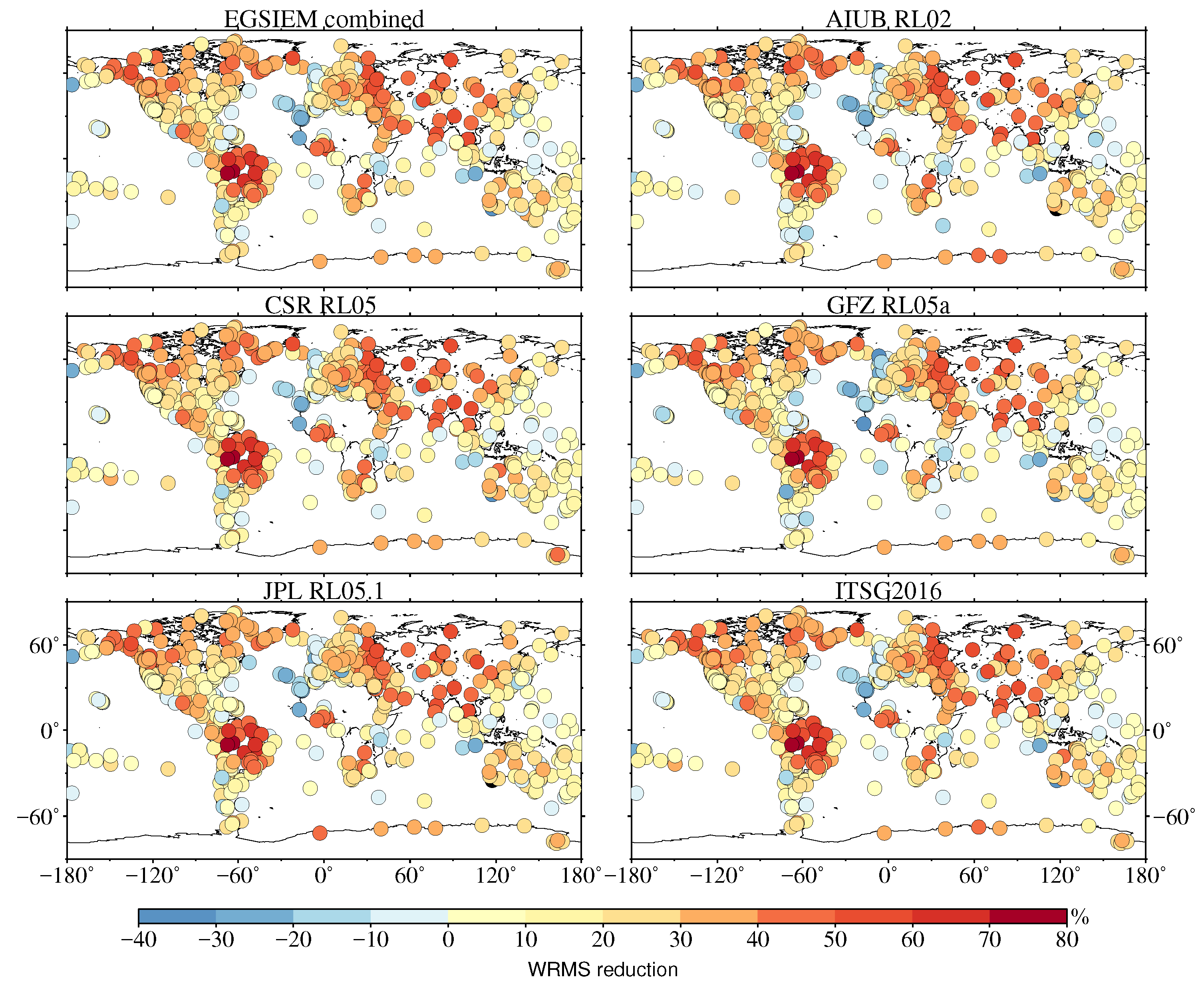
4.1. Full Signal Level

We commence the validation by showing the mean degree WRMS reductions and cumulative degree WRMS reductions of the six considered gravity solutions using the ITRF2014 residuals over 928 GNSS stations globally in Figure 1. Inspection of the mean degree WRMS reductions in Figure 1b, it is clear that the lower spherical harmonic degrees of the gravity fields contribute largely to the total WRMS reductions. Degree-2 and degree-3 share the most significant contributions. It is interesting to observe that different gravity solutions show slightly different performances at each SH degree. For example, CSR RL05 seems to agree visually better at degree-2 using both the ITRF2014 residuals as well as the EGSIEM-reprocessed GNSS time series (see Figure S1).
Figure 1b presents the mean cumulative degree WRMS reductions for all the GRACE solutions. The EGSIEM combined solutions, ITSG2016 and CSR RL05, show very close performances and are slightly better than other solutions. GFZ RL05a provides marginally worse cumulative WRMS reductions which might be due to its inferior performance at degree-3, which is also observed by using the other two GNSS time series from EGSIEM-reprocessed (see Figure S1) and JPL (see Figure S5). Nevertheless, the mean cumulative WRMS reductions shown here from all six gravity solutions are better than that from the latest results (maximum mean WRMS reduction up to 15%, see Table S3) published by Gu et al. (2017) [9]. One more feature to be gleaned from Figure 1 is that no significant contributions come from degree beyond 30, which has been already demonstrated by Han (2016) [45].
The spatial plots showing correlations between GNSS-observed and GRACE-derived displacements are presented in Figure 2. In terms of spatial correlation plots, all gravity solutions depict similar patterns with colors in red to pink clearly dominating implying excellent consistency between GNSS and GRACE. To be more specific, GNSS stations located in the continent exhibit strong correlations, especially in the regions like the Amazonian area where the most significant water mass variations happen. While the stations located at islands or close to the coast display lower or even negative correlations, i.e., light yellow to cyan colors, which are possibly affected by non-tidal oceanic loading effects [8,46,47] or even spurious long-period signals due to unmodeled short-periodic displacements [48].
Besides the correlation maps, the WRMS reduction maps of the gravity solutions up to their full spectrum are shown in Figure 3. As seen clearly from Figure 3, yellow to red colors are overwhelmingly predominant confirming the strong agreement between GNSS and GRACE. The highest WRMS reduction is observed at the POVE station located in Porto Velho, Brazil with a reduction of 78.1% using the EGSIEM combined solutions. Note that this percentage varies with different GNSS datasets. For example, the highest WRMS reduction using the ITRF2014 residuals is 76.3% at the same station.
The WRMS reductions on all three GNSS datasets (Figure 3, Figure S2, and Figure S6) using the different gravity field solutions are summarized in Table 1. Note that there are different numbers of stations from the three GNSS datasets shown in the table. The aim of Table 1 is to evaluate the performances of different gravity solutions under different GNSS datasets. Statistically, the EGSIEM combined solutions perform overwhelmingly good using the three different GNSS datasets. The EGSIEM combined solutions together with CSR RL05 and ITSG2016 show consistently close performances and slightly outperform the other three gravity solutions. It is worth mentioning again that ITSG2014 instead of the latest ITSG2016 was involved in the combination process to generate our EGSIEM-combined long term monthly solutions [3]. In addition, the EGSIEM combined long term solutions were produced as long as any monthly gravity solutions exist. To a certain extent, these two factors might degrade the performance of the combined solutions.
Table 1 also shows that differences of the statistics (mean and positive WRMS reductions) using the same GNSS dataset but different GRACE solutions are less than that of using different GNSS datasets but the same GRACE products. This phenomenon is also supported by the below-mentioned Table 2 and Table 3. These tables indicate that the differences among different GNSS products are larger than the differences among different gravity field solutions, which has also been suggested by Gu et al. (2017) [9] who compared multi-institutional GNSS and GRACE products. In other words, the GRACE products are more consistent with one another than the GNSS products. Nevertheless, regardless of different GNSS products with different number of stations used in this study, performances of the evaluated GRACE solutions tend to be consistent, which ensures the robustness of our validation.

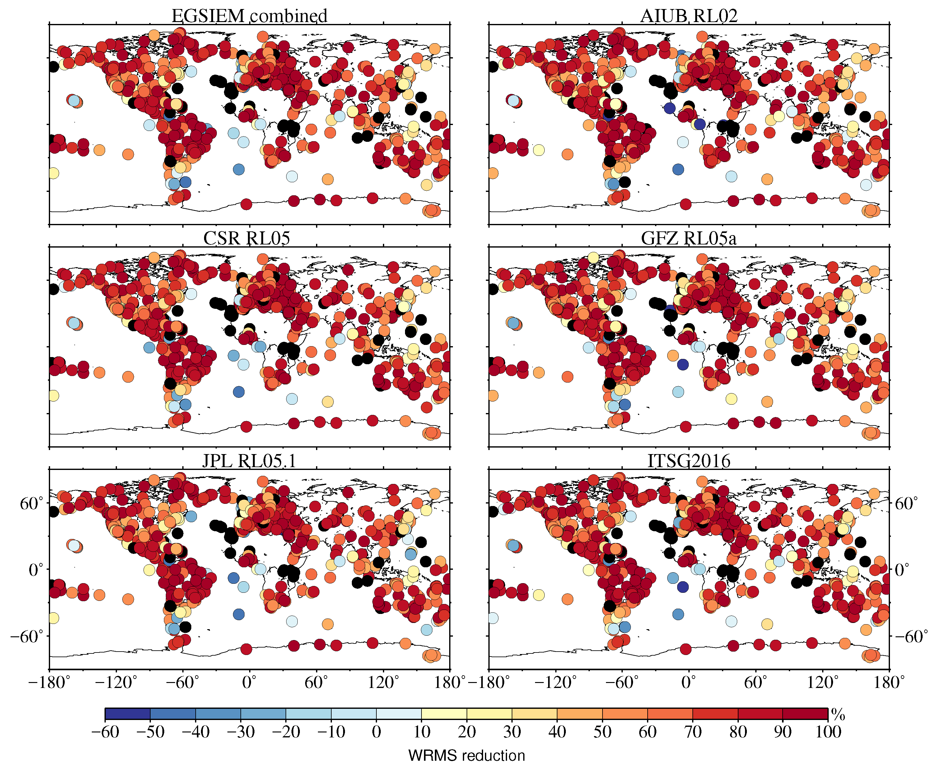
4.2. Annual Signal Level

Apart from the validation of the gravity fields at the full signal level, the performances of the six considered gravity solution are evaluated at the annual period. Figure 4 presents the median degree and cumulative degree WRMS reductions at the annual signal level. Similarly, low SH degrees representing the long-wavelength mass variations display significant WRMS reductions indicating high agreements between GNSS-observed and GRACE-derived vertical displacements at the annual period. This is because the annual signals in GNSS and GRACE are driven by annual variations in the water cycle that is a long-wavelength effect. The bottom panel of Figure 4 exhibits up to median values of 70% WRMS reductions for all six gravity fields when using the ITRF2014 dataset in the comparison.
These phenomena are observed as well in the spatial plots shown in Figure 5. A large number of GNSS stations show high WRMS reductions (light red to dark red colors) at the annual signal level indicating remarkably good agreement between GNSS and GRACE. The statistics at the annual period from the three GNSS products (Figure 5, Figure S4, and Figure S8) are shown in Table 2 confirming the above-mentioned finding that the discrepancies among the different GNSS datasets are more significant than those of the different gravity solutions. At the annual period, the maximum difference of the median WRMS reductions among three GNSS datasets using the same GRACE product (GFZ RL05a) is 15.7% which is much larger than 6.3% the maximum difference of the median WRMS reductions among different gravity solutions using the same GNSS dataset (JPL GNSS time series).

4.3. Validation over Common GNSS Stations

In this subsection, we compare the different GNSS data products using the GRACE products. We extract the common GNSS stations from the three GNSS data products and summarize their statistics in Table 3. A common set of 236 GNSS stations is used.
The WRMS reductions presented in Table 3 show that removing the GRACE signals from the EGSIEM-reprocessed GNSS products are very similar with the ITRF2014 residuals having slightly larger WRMS reduction percentages. The WRMS reduction percentages for the JPL GNSS time series, which are claimed to be clean and detrended, are lower than for the EGSIEM-reprocessed and the ITRF2014 GNSS data. A careful post-processing to remove unresolved offsets and outliers is recommended for using these JPL GNSS time series. In addition, Table 3 demonstrates again the conclusion that different GNSS products show larger differences than different GRACE products when comparing between GNSS and GRACE products. That is too say, the inconsistencies between GNSS and GRACE are most likely due to errors in the GNSS data like site-specific effects [6,8,9].

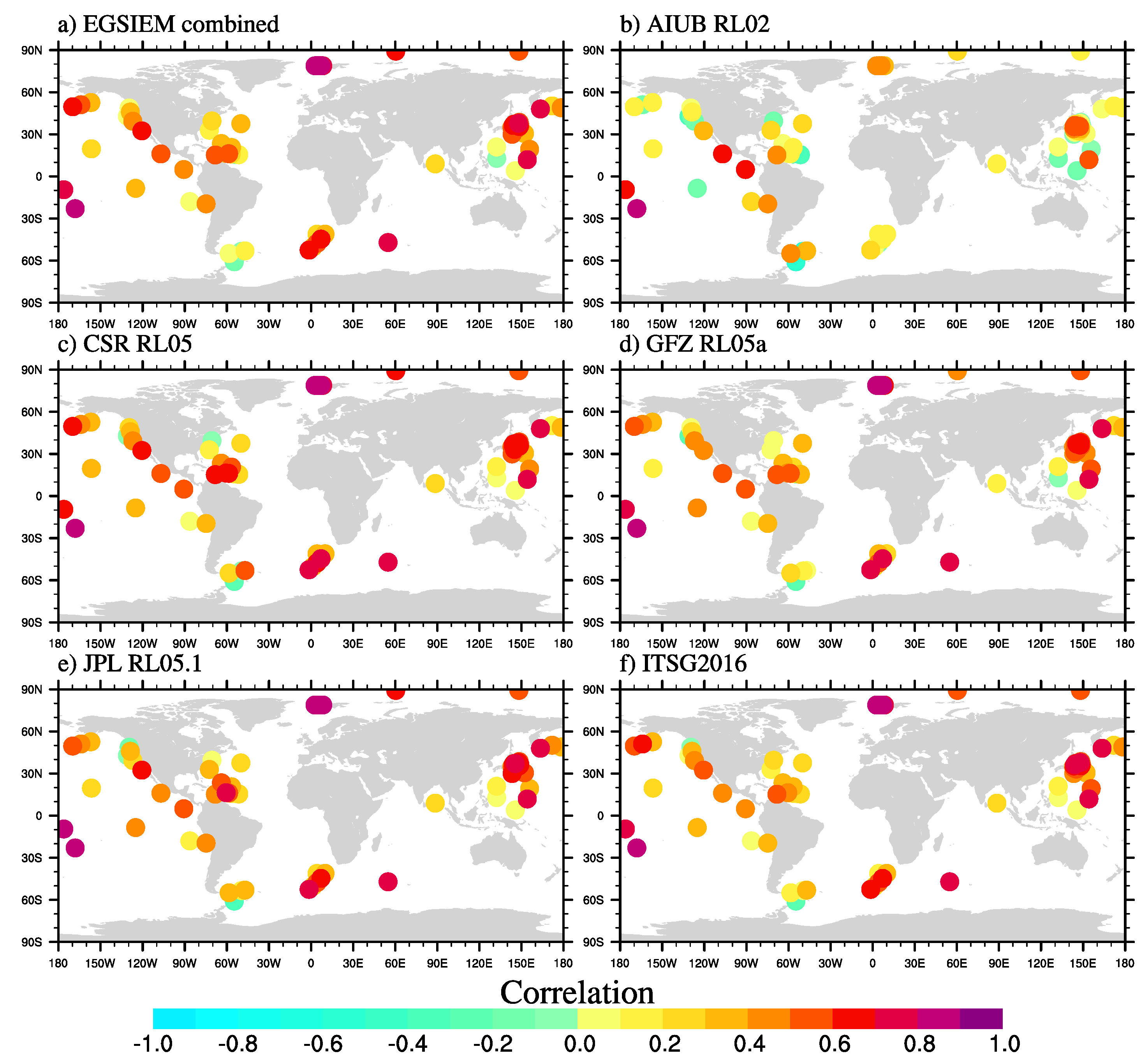
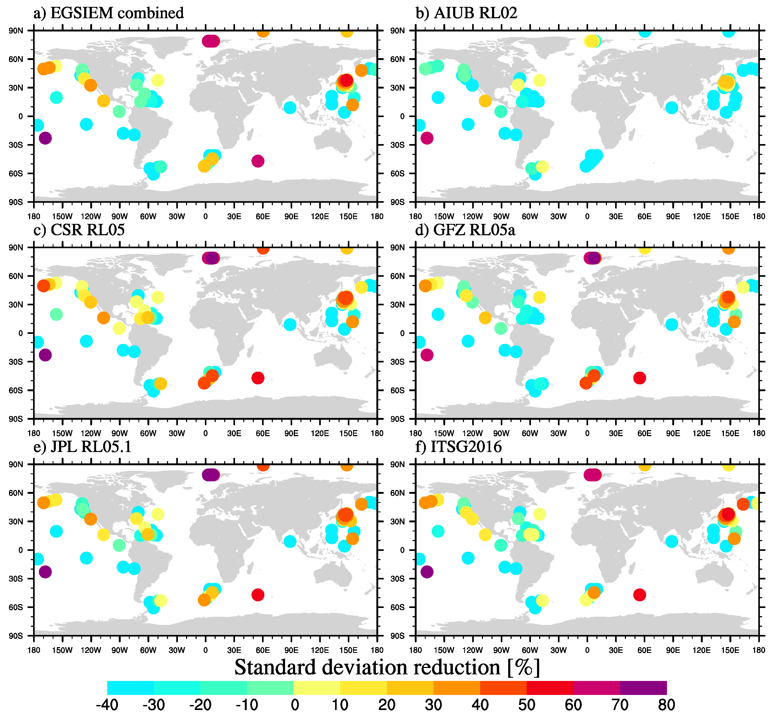
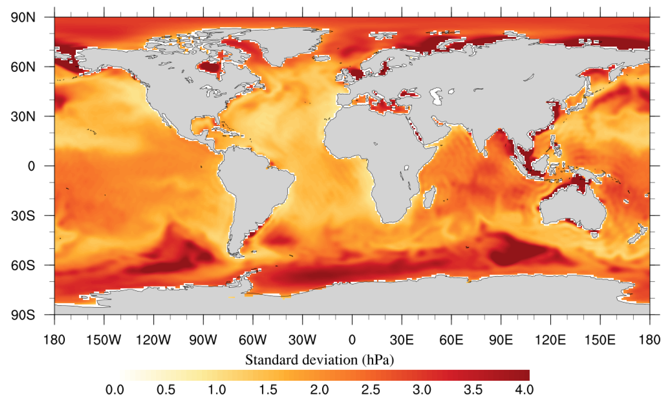
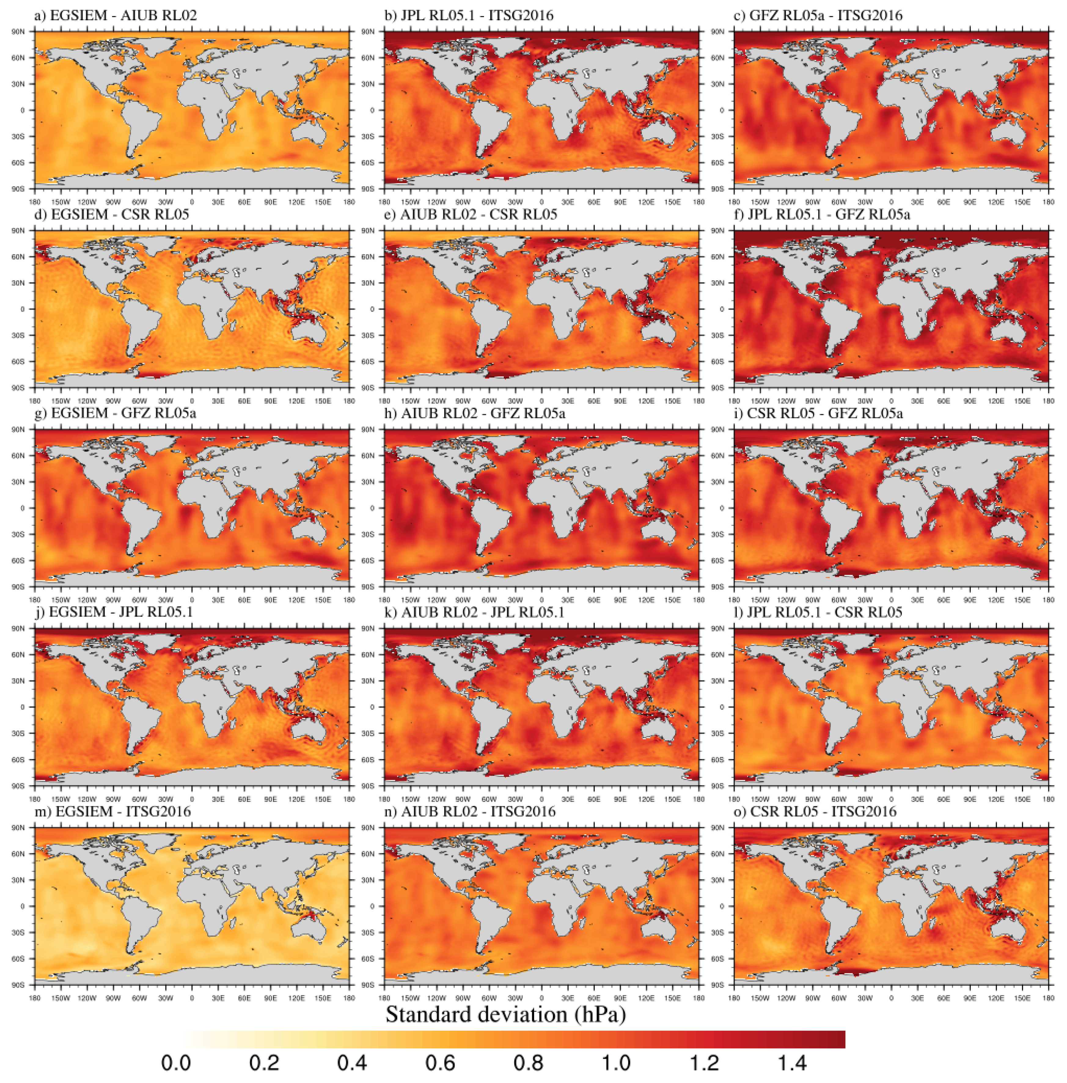
5. Validation Using OBP Records

In this section, we use time series from 103 globally distributed in-situ OBP stations that have sufficient data to allow us to calculate at least 12 monthly averages. For the AIUB RL02 comparison, some OBP time series are discarded so that the number of OBP time series is reduced to 98. This is because the AIUB RL02 GRACE dataset contains less monthly solutions than the other GRACE datasets used here.
The correlation (Figure 6) between different GRACE solutions and the in-situ OBP data is significantly lower than the correlation of GRACE and GNSS datasets over the continents. Still the correlations are comparable or even slightly better than the correlation with GNSS data on islands and close to the coasts. In general, correlations are positive at the OBP stations. Less than ten negative correlations are observed where most of those are in the vicinity of the coasts. The only exception to that result is the AIUB RL02 GRACE solution, which has over 30 locations with negative correlations. The highest correlation ranges between 0.81 for the AIUB RL02 GRACE solution and 0.90 for the JPL RL05.1 solution. There are two locations with such high correlations for all studied GRACE solutions: in Greenland Sea, where GFZ, JPL, and ITSG solutions have their maximum correlation values, and in the Central Pacific Ocean, where the CSR, AIUB, and the EGSIEM combined solution have the highest correlations. Both locations have relatively high variability of OBP and the regions of coherent variability calculated for in-situ stations in those areas are very large, which is why the in-situ time series can be considered representative for the whole region, resulting in very high correlation between area-averaging GRACE and in-situ data. Again, in terms of correlations, all GRACE gravity field solutions show very similar geographical patterns.
As seen from Figure 7, the standard deviation reductions on the OBP time series after removing the GRACE pressure signal are much lower compared to the WRMS reductions on the GNSS time series (Figure 3). Unlike the WRMS reductions on GNSS data, the standard deviation reductions on the in-situ OBP data are lower and sometimes negative for the majority of the OBP time series. This result is expected since the monthly GRACE fields are dominated by seasonal and interannual signals driven by temporal variations in terrestrial water storage and ice mass. In comparison to those signals, the variability in ocean bottom pressure is much smaller and, consequently, the signal to noise ratio in GRACE is lower. Furthermore, because the OBP variability is much higher for the submonthly frequency bands, which causes aliasing in the GRACE monthly solutions, those signals have been removed by means of de-aliasing models, whose errors cause aliasing artifacts over the oceans. Another possible reason for such low agreement between the GRACE and the in-situ OBP data might be the removal of trends from both datasets, which had to be performed because it is very difficult to determine which trends in the in-situ time series are real and which are the result of sensor drifts. Since the majority of time series do not cover the whole timespan of the GRACE time series, the trends removed from the in-situ and from the GRACE observations are sometimes different.
When looking at the STD reduction plots (Figure 7), it is nevertheless easier to discriminate between different GRACE solutions than from the correlations. While the geographic patterns are again similar, i.e., better agreement between the GRACE and the in-situ data in the higher latitudes than in the equatorial regions where the signal is lower and the GRACE time series are dominated by noise (as shown in Figure 8), there are some noticeable differences between the GRACE solutions. In the North Atlantic Ocean most GRACE solutions have negative STD reductions, whereas the CSR RL05 solution has a large number of positive values. The AIUB RL02 solutions are the only gravity solutions with negative STD reductions near the North pole, where all other solutions have positive and usually relatively high reductions. EGSIEM and CSR solutions have mostly positive (even above 30%) values along the western North American coast, where the other solutions have a lot lower and mostly negative values. The highest STD reduction is around 50% for all GRACE solution and is located at the same two regions with the highest correlation, i.e., the Greenland Sea and the Central Pacific Ocean. Based on these differences on the STD reduction maps we conclude that CSR RL05, ITSG2016, and the EGSIEM combined solutions outperform the other three GRACE timeseries in this study.
The summary of the comparison of the GRACE solutions with in-situ OBP is given in Table 4. As expected the mean values for all GRACE gravity field solutions are negative due to the large number of stations with negative STD reductions. The highest mean STD reduction is −5.5% for the ITSG2016 GRACE solution, closely followed by the JPL, CSR, and EGSIEM combined solution. When considering only the positive reductions, the values are still lower than the WRMS reductions with GNSS data. Here, EGSIEM has the highest mean value of 18.3%, closely followed by the JPL and ITSG solutions.
In addition to the comparison of the GRACE solutions against in-situ OBP, it is also indicative to look at the pairwise differences between the GRACE solutions from different processing centres (Figure 9). As expected, because the EGSIEM combined solutions are combined from the others, the differences between EGSIEM and the other 5 solutions are significantly smaller than the differences between the other pairs of GRACE solutions. The differences are the smallest for the ITSG2016 solution (approximately 0.5 hPa), followed by the CSR RL05 and AIUB RL02 solutions, which both have standard deviation of differences up to 0.8 hPa in the open ocean. The differences between the GFZ RL05a and other solutions are the highest, often exceeding 1.5 hPa.

6. Discussion

6.1. Comparison to the Previous Comparison Studies of GNSS and GRACE

A number of previous studies have compared GNSS observed and GRACE-derived vertical displacements at the global scale e.g., [7,8,9,10]. Compared to these studies, this study has shown better statistical results. In comparison to the earlier studies by Tregoning et al. (2009) [7] and Tesmer et al. (2011) [8], we have found more than 85% positive WRMS reductions from 928 global GNSS stations with regards to 50% out of 80 global sites [7] and around 80% out of 115 sites [8]. This result is expected as we have used both improved GNSS data and GRACE data in our validation process. For example, in terms of the GRACE data, official GRACE RL04 products were used in Tesmer et al. (2011) while we have used the GRACE RL05 products.
In a very recent study of comparing multiple GNSS and GRACE products in the up direction, Gu et al. (2017) [9] found maximum mean WRMS up to 15% using the ITSG2016 GRACE products and the JPL GNSS products. In the latest study by Chanard et al. (2018) [10], they compared the ITRF2014 residuals of 689 global stations to the GRGS RL03 GRACE products and obtained the maximum WRMS reduction of 14.7% in the vertical component. With respect to these two recent studies, we have found larger mean WRMS reductions up to 25.6% using the ITSG2016 GRACE gravity fields and the ITRF2014 residuals. Comparing to Gu et al. (2017) [9], our ITRF2014 residuals are the combined solutions out of the multiple GNSS products used by Gu et al. (2017) [9] during the second IGS data reprocessing compaign [40], which probably makes our results better. With regard to Chanard et al. (2018), we have not used GRGS RL03 gravity products in our study due to the fact that GRGS RL03 solutions require no further post-processing, e.g., replacement of C20 and filtering. To a large extent, those post-processing steps affect the WRMS reduction results. For instance, in our study, we have applied a relatively strong filter (the Gaussian filter with the smoothing radius of 500 km) as GRACE and GNSS agree better at longer periods.
At the annual signal level, we have used different evaluation metrics. For example, Gu et al. (2017) [9] obtained maximum around 50% mean reduction of annual amplitude while we have found up to 73% median WRMS reduction of the time series. Nevertheless, our results at the annual signal level are comparible.

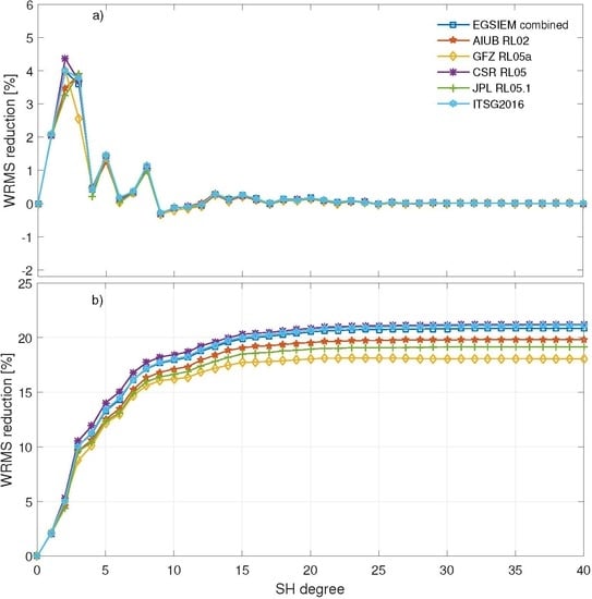
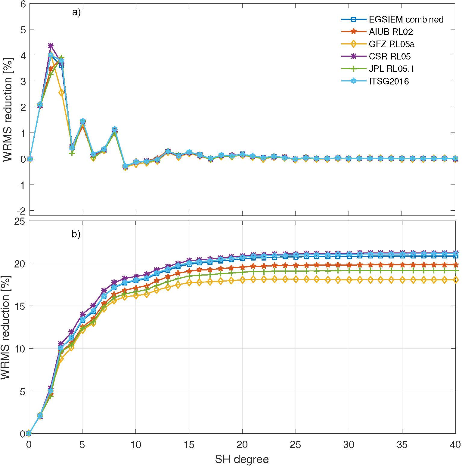
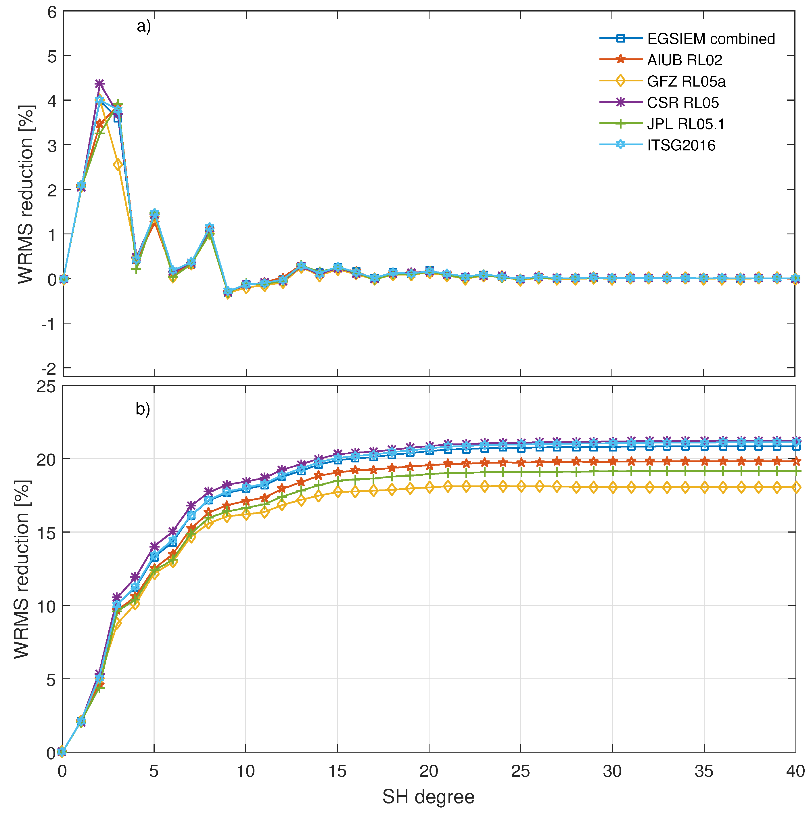
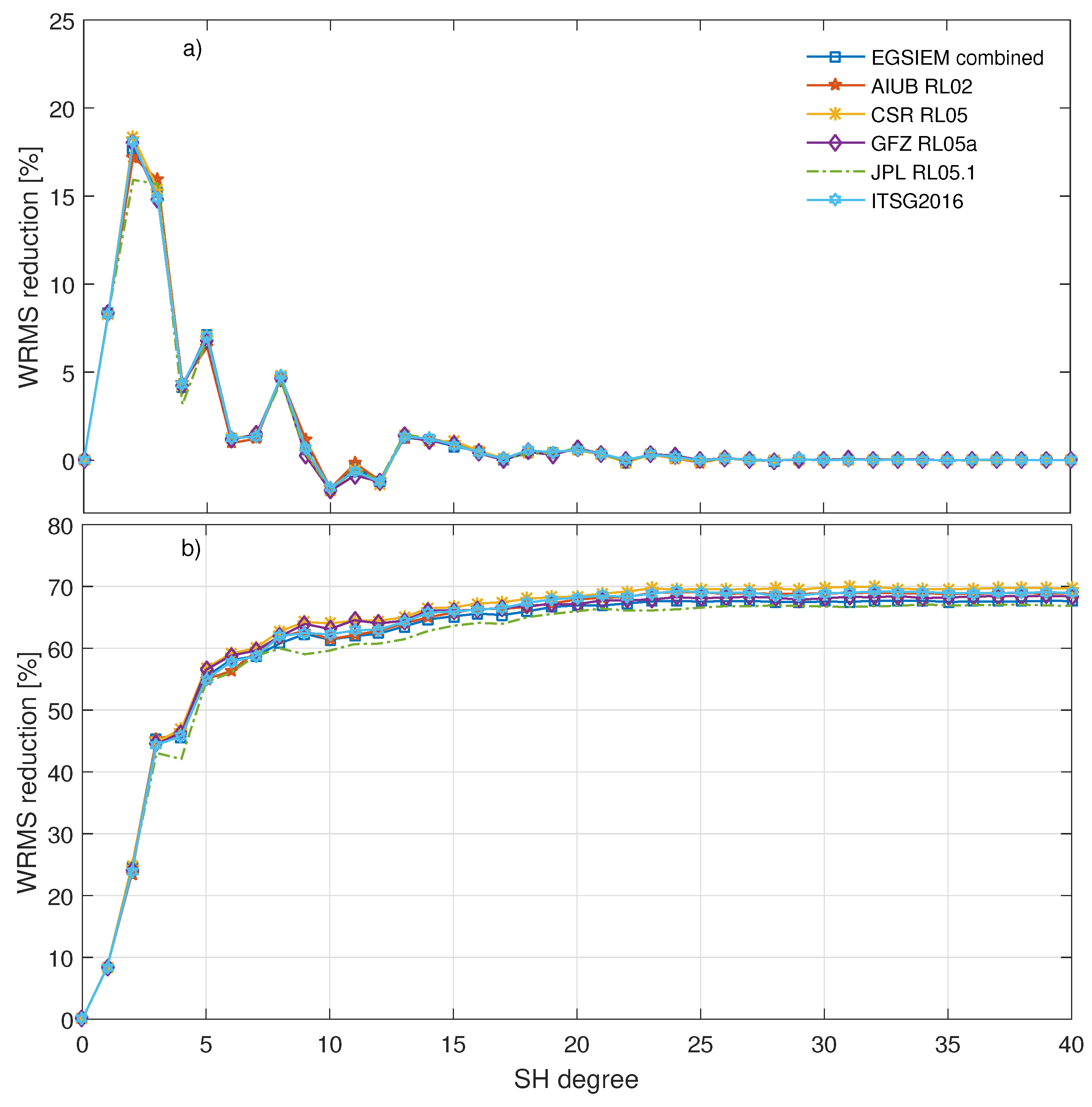
6.2. Degree and Cumulative Degree WRMS Reductions

Conventionally, WRMS reduction e.g., [6,7,8,9,10] has been considered as one important metric in the community when comparing GNSS and GRACE. Within the EGSIEM project we have introduced the degree WRMS reduction and cumulative degree WRMS reduction metrics in our GNSS validation process allowing us to evaluate the performance of each spherical harmonic degree of the GRACE products separately. These two metrics are particularly helpful when unusual behaviors appear in the lower spherical harmonic degrees of the GRACE products. For example, we have found the abnormal behavior at degree 2 of the EGSIEM-GRGS solutions by using the degree WRMS reduction metric (see Figure 8 in [2]). Via further degree WRMS reduction analysis at each coefficient of degree 2, we have been able to track the degree-2 problem of the EGSIEM-GRGS solutions down to be caused by C 21 and S 21 terms. This problem would not have been clear using the WRMS reduction alone.
Through the degree and cumulative degree WRMS reduction analysis, we observe different WRMS reductions at lower spherical harmonic coefficients using different GNSS datasets, which contribute most to the total WRMS reduction when investigating both the full signal and the annual signals (see Figure 1, Figure S1, Figure S3, Figure 4, Figure S5, and Figure S7). In particular, we replace the C 20 terms and restore the degree-1 coefficients to GRACE in post-processing of the GRACE spherical harmonic products. Different degree-1 coefficients and C 20 terms will affect the comparison between GNSS and GRACE. For example, experiments have been implemented during the EGSIEM project using the external degree-1 coefficients from Swenson et al. (2008) [32] and Sośnica et al. (2015) [49], and noticeable differences are observed at both the full and annual signal comparisons. Further investigation to understand the impacts of degree-1 and C 20 terms is necessary for both the current GRACE as well as GRACE Follow-on gravity products [50]. In addition, the EGSIEM combination service will be continued as the International Combination Service for Time-variable Gravity fields (COST-G) under the umbrella of the International Gravity Field Service (IGFS) [2]. Future validation of the combined gravity fields using the latest GRACE Release 6 products [51] via the degree and cumulative degree WRMS reductions will be of great importance as well.

6.3. Consistency of Validation between GNSS and OBP

Another valuable feature of our validation process using both GNSS and OBP lies in the consistency between both validation techniques. Both validation techniques confirm that CSR RL05, ITSG2016, and the EGSIEM-combined solutions reduce scatters on GNSS or OBP at a comparable level and to a greater extent than the other three solutions, i.e., AIUB RL02, GFZ RL05a, and JPL RL05.1. The only exception is that JPL RL05.1 performs well considering all available in-situ OBP records but slightly worse in terms of validation using GNSS. One possible reason might be the shorter GRACE data (2003–2010 only) used during the validation by OBP since only shorter time-span in-situ OBP records are available.

7. Conclusions

As an essential part of the EGSIEM project, this study has successfully demonstrated the capabilities of the GNSS time series and in-situ OBP records for validating GRACE monthly gravity fields. We have shown that both validation techniques are able to evaluate the quality of different gravity series.
By comparing the six monthly gravity field products to the three independent GNSS datasets, we can conclude that strong agreements between GNSS and GRACE have been clearly observed at both the full and the annual signals. Depending on the GNSS products, up to 25.6% mean WRMS reduction is obtained comparing GRACE to the ITRF2014 residuals over 236 GNSS stations. At the annual signal level, up to 73% median WRMS reduction is found comparing GRACE to the 312 EGSIEM-reprocessed GNSS time series. With the help of the degree and cumulative degree WRMS reduction metrics introduced in this study, strong contributions from the lower spherical harmonic degrees are observed. In addition, the EGSIEM-combined solutions are comparable to the ITSG2016 and CSR RL05 monthly solutions, and slightly better than other three monthly solutions, i.e., AIUB RL02, GFZ RL05a, and JPL RL05.1. A comparison of GNSS and GRACE over the 236 common GNSS stations indicates a good performance of the EGSIEM-reprocessed GNSS datasets as well.
Validation of the gravity fields using the OBP records confirms the conclusions found using GNSS although the agreement with the in-situ OBP is generally worse than the agreement with the GNSS datasets. While the correlations between GRACE and the in-situ OBP time series are mostly positive and relatively high, they only slightly differ among the GRACE solutions. The STD reductions are mostly negative for all studied GRACE solutions, but from the sample of positive stations, it is possible to determine that the CSR RL05, ITSG2016, and EGSIEM-combined solution are slightly better than the remaining three GRACE solutions.

Supplementary Materials

The following are available online at https://www.mdpi.com/2072-4292/10/12/1976/s1. Figure S1: Mean degree WRMS reductions and cumulative degree WRMS reductions of different gravity solutions using the EGSIEM-reprocessed GNSS data over 312 GNSS stations globally at the full signal level, Figure S2: WRMS reduction at the full signal over 312 GNSS stations using the EGSIEM-reprocessed GNSS data, Figure S3: Median degree WRMS reductions and cumulative degree WRMS reductions of different gravity solutions using the EGSIEM-reprocessed GNSS data at the annual signal level over 312 GNSS stations globally, Figure S4: WRMS reduction at the annual signal over 312 GNSS stations using the EGSIEM-reprocessed GNSS data, Figure S5: Mean degree WRMS reductions and cumulative degree WRMS reductions of different gravity solutions using the JPL GNSS time series over 788 GNSS stations globally at the full signal level, Figure S6: WRMS reduction at the full signal over 788 GNSS stations using the JPL GNSS time series, Figure S7: Median degree WRMS reductions and cumulative degree WRMS reductions of different gravity solutions using the JPL GNSS time series at the annual signal level over 788 GNSS stations globally, Figure S8: WRMS reduction at the annual signal over 788 GNSS stations using the JPL GNSS time series.

Author Contributions

Q.C., H.D. and M.W. conceived and designed the experiments; Q.C. and L.P. performed the experiments; Q.C., L.P. and L.Z. analyzed the data; Q.C. and L.P. wrote the paper. L.Z., H.D., M.W. and T.v.D. provided critical comments on the manuscript.

Funding

This research was supported by the European Union’s Horizon2020 research and innovation program under the Grant Agreement No.637010.

Acknowledgments

We are grateful to Paul Rebischung from IGN (France) and JPL (USA) for providing us the GNSS products. We thank Andreas Macrander from MFRI (Marine and Freshwater Research Institute, Reykjavik, Iceland) for compiling and sharing his OBP database. MPIOM model data is accessible from isdc.gfz-potsdam.de/esmdata. MPIOM simulations were performed at Deutsches Klimarechenzentrum in Hamburg, Germany.

Conflicts of Interest

The authors declare no conflict of interest.

Abbreviations

The following abbreviations are used in this manuscript:
ACAnalysis Center
AIUBAstronomical Institute, University of Bern
COST-GInternational Combination Service for Time-variable Gravity fields
CSRCenter for Space Research, Austin, Texas
EGSIEMEuropean Gravity Service for Improved Emergency Management
EUEuropean Union
GACGeopotential coefficients of averaged combination of non-tidal atmosphere and ocean
GADGeopotential coefficients of averaged combination of bottom pressure over oceans
GFZHelmholtz Centre Potsdam, German Research Centre for Geosciences
GIAGlobal Isostatic Adjustment
GGMGlobal Geopotential Model
GNSSGlobal Navigation Satellite System
GPSGlobal Positioning System
GRACEGravity Recovery and Climate Experiment
GSMGeopotential coefficients of GRACE-derived gravity field
IGFSInternational Gravity Field Service
IGSInternational GNSS Service
ITRFInternational Terrestrial Reference Frame
JPLJet Propulsion Laboratory, Pasadena, California, USA
KESSKuroshio Extension System Study
MPIOMMax Planck Institute Ocean Model
NEUNorth East Up
OBPOcean Bottom Pressure
RMSRoot Mean Square
SHCSpherical Harmonic Coefficient
SLRSatellite Laser Ranging
STDStandard Deviation
UBERNUniversity of Bern
WRMSWeighted Root-Mean-Square

References

  1. Tapley, B.D.; Bettadpur, S.; Ries, J.C.; Thompson, P.F.; Watkins, M.M. GRACE Measurements of Mass Variability in the Earth System. Science 2004, 305, 503–505. [Google Scholar] [CrossRef] [PubMed] [Green Version]
  2. Jäggi, A. European Gravity Service for Improved Emergency Management (EGSIEM)-from concept to implementation. Geophys. J. Int. 2018. submitted. [Google Scholar]
  3. Jean, Y.; Meyer, U.; Jäggi, A. Combination of GRACE monthly gravity field solutions from different processing strategies. J. Geod. 2018, 1–16. [Google Scholar] [CrossRef]
  4. Meyer, U.; Jean, Y.; Jäggi, A. Combination of GRACE monthly gravity fields on normal equation level. J. Geod. 2018. submitted. [Google Scholar]
  5. Davis, J.L.; Elósegui, P.; Mitrovica, J.X.; Tamisiea, M.E. Climate-driven deformation of the solid Earth from GRACE and GPS. Geophys. Res. Lett. 2004, 31, L24605. [Google Scholar] [CrossRef]
  6. van Dam, T.; Wahr, J.; Lavallée, D. A comparison of annual vertical crustal displacements from GPS and Gravity Recovery and Climate Experiment (GRACE) over Europe. J. Geophys. Res. 2007, 112, B03404. [Google Scholar] [CrossRef]
  7. Tregoning, P.; Watson, C.; Ramillien, G.; McQueen, H.; Zhang, J. Detecting hydrologic deformation using GRACE and GPS. Geophys. Res. Lett. 2009, 36, L15401. [Google Scholar] [CrossRef]
  8. Tesmer, V.; Steigenberger, P.; van Dam, T.; Mayer-Gürr, T. Vertical deformations from homogeneously processed GRACE and global GPS long-term series. J. Geod. 2011, 85, 291–310. [Google Scholar] [CrossRef]
  9. Gu, Y.; Fan, D.; You, W. Comparison of observed and modeled seasonal crustal vertical displacements derived from multi-institution GPS and GRACE solutions. Geophys. Res. Lett. 2017, 44, 7219–7227. [Google Scholar] [CrossRef]
  10. Chanard, K.; Fleitout, L.; Calais, E.; Rebischung, P.; Avouac, J.P. Toward a Global Horizontal and Vertical Elastic Load Deformation Model Derived from GRACE and GNSS Station Position Time Series. J. Geophys. Res. Solid Earth 2018, 123, 3225–3237. [Google Scholar] [CrossRef]
  11. Fu, Y.; Freymueller, J.T.; Jensen, T. Seasonal hydrological loading in southern Alaska observed by GPS and GRACE. Geophys. Res. Lett. 2012, 39, L15310. [Google Scholar] [CrossRef]
  12. Chen, Q. Analyzing and Modmodel Environmental Loading Induced Displacements with GPS and GRACE. Ph.D. Thesis, University of Stuttgart, Stuttgart, Germany, 2015. [Google Scholar]
  13. Chambers, D.P.; Wahr, J.; Nerem, R.S. Preliminary observations of global ocean mass variations with GRACE. Geophys. Res. Lett. 2004, 31, L13310. [Google Scholar] [CrossRef]
  14. Kanzow, T.; Flechtner, F.; Chave, A.; Schmidt, R.; Schwintzer, P.; Send, U. Seasonal variation of ocean bottom pressure derived from Gravity Recovery and Climate Experiment (GRACE): Local validation and global patterns. J. Geophys. Res. 2005, 110. [Google Scholar] [CrossRef] [Green Version]
  15. Rietbroek, R.; LeGrand, P.; Wouters, B.; Lemoine, J.M.; Ramillien, G.; Hughes, C.W. Comparison of in situ bottom pressure data with GRACE gravimetry in the Crozet-Kerguelen region. Geophys. Res. Lett. 2006, 33. [Google Scholar] [CrossRef] [Green Version]
  16. Dobslaw, H.; Flechtner, F.; Bergmann-Wolf, I.; Dahle, C.; Dill, R.; Esselborn, S.; Sasgen, I.; Thomas, M. Simulating high-frequency atmosphere-ocean mass variability for dealiasing of satellite gravity observations: AOD1B RL05. J. Geophys. Res. Oceans 2013, 118, 3704–3711. [Google Scholar] [CrossRef] [Green Version]
  17. Dobslaw, H.; Bergmann-Wolf, I.; Dill, R.; Poropat, L.; Thomas, M. A new high-resolution model of non-tidal atmosphere and ocean mass variability for de-aliasing of satellite gravity observations: AOD1B RL06. Geophys. J. Int. 2017, 211, 263–269. [Google Scholar] [CrossRef] [Green Version]
  18. Poropat, L.; Dobslaw, H.; Zhang, L.; Macrander, A.; Boebel, O.; Thomas, M. Time variations in ocean bottom pressure from a few hours to many years: In situ data, numerical models, and GRACE satellite gravimetry. J. Geophys. Res. Oceans 2018, 123, 5612–5623. [Google Scholar] [CrossRef]
  19. Ray, J.; Altamimi, Z.; Collilieux, X.; van Dam, T. Anomalous harmonics in the spectra of GPS position estimates. GPS Solut. 2008, 12, 55–64. [Google Scholar] [CrossRef]
  20. Ray, J.; Griffiths, J.; Collilieux, X.; Rebischung, P. Subseasonal GNSS positioning errors. Geophys. Res. Lett. 2013, 40, 5854–5860. [Google Scholar] [CrossRef] [Green Version]
  21. van Dam, T.M.; Blewitt, G.; Heflin, M.B. Atmospheric pressure loading effects on Global Positioning System coordinate determinations. J. Geophys. Res. 1994, 99, 23939–23950. [Google Scholar] [CrossRef]
  22. van Dam, T.; Wahr, J.; Milly, P.C.D.; Shmakin, A.B.; Blewitt, G.; Lavallée, D.; Larson, K.M. Crustal displacements due to continental water loading. Geophys. Res. Lett. 2001, 28, 651–654. [Google Scholar] [CrossRef] [Green Version]
  23. Farrell, W.E. Deformation of the Earth by surface loads. Rev. Geophys. 1972, 10, 761–797. [Google Scholar] [CrossRef]
  24. Wahr, J.; Molenaar, M.; Bryan, F. Time variability of the Earth’s gravity field: Hydrological and oceanic effects and their possible detection using GRACE. J. Geophys. Res. 1998, 103, 30205–30229. [Google Scholar] [CrossRef]
  25. Mayer-Gürr, T.; Zehentner, N.; Klinger, B.; Kvas, A. ITSG-Grace2014: A new GRACE gravity field release computed in Graz. In Proceedings of the GRACE Science Team Meeting (GSTM), Potsdam, Germany, 29 Sepember–1 October 2014. [Google Scholar]
  26. Mayer-Gürr, T.; Behzadpour, S.; Ellmer, M.; Kvas, A.; Klinger, B.; Zehentner, N. ITSG-Grace2016–Monthly and Daily Gravity Field Solutions from GRACE. GFZ Data Services, 2016. Available online: https://graz.pure.elsevier.com/en/publications/itsg-grace2016-monthly-and-daily-gravity-field-solutions-from-gra (accessed on 20 August 2018).
  27. Bettadpur, S. UTCSR Level-2 Processing Standards Document; Technical Report; Center for Space Research, University of Texas: Austin, TX, USA, 2012. [Google Scholar]
  28. Dahle, C.; Flechtner, F.; Gruber, C.; König, D.; König, R.; Michalak, G.; Neumayer, K. GFZ GRACE Level-2 Processing Standards Document for Level-2 Product Release 005; GFZ Data Services: Potsdam, Germany, 2012. [Google Scholar]
  29. Watkins, M.; Yuan, T.D. JPL Level-2 Processing Standards Document for Level-2 Product Release 05; Technical Report; NASA JPL: Pasadena, CA, USA, 2012.
  30. Meyer, U.; Jäggi, A.; Jean, Y.; Beutler, G. AIUB-RL02: An improved time series of monthly gravity fields from GRACE data. Geophys. J. Int. 2016. [Google Scholar] [CrossRef]
  31. Cheng, M.; Tapley, B.D.; Ries, J.C. Deceleration in the Earth’s oblateness. J. Geophys. Res. Solid Earth 2013, 118, 740–747. [Google Scholar] [CrossRef]
  32. Swenson, S.; Chambers, D.; Wahr, J. Estimating geocenter variations from a combination of GRACE and ocean model output. J. Geophys. Res. 2008, 113, B08410. [Google Scholar] [CrossRef]
  33. Blewitt, G. Self-consistency in reference frames, geocenter definition, and surface loading of the solid Earth. J. Geophys. Res. 2003, 108, 2103. [Google Scholar] [CrossRef]
  34. Jekeli, C. Alternative Methods to Smooth the Earth’s Gravity Field; Technical Report 327; Department of Geodetic Science and Surveying, The Ohio State University: Columbus, OH, USA, 1981. [Google Scholar]
  35. Bergmann-Wolf, I.; Zhang, L.; Dobslaw, H. Global Eustatic Sea-Level Variations for the Approximation of Geocenter Motion from Grace. J. Geod. Sci. 2014, 4, 37–48. [Google Scholar] [CrossRef]
  36. Paulson, A.; Zhong, S. Inference of mantle viscosity from GRACE and relative sea level data. Geophys. J. Int. 2007, 171, 497–508. [Google Scholar] [CrossRef] [Green Version]
  37. Tanaka, Y.; Suzuki, T.; Imanishi, Y.; Okubo, S.; Zhang, X.; Ando, M.; Watanabe, A.; Saka, M.; Kato, C.; Oomori, S.; et al. Temporal gravity anomalies observed in the Tokai area and a possible relationship with slow slips. Earth Planets Space 2018, 70. [Google Scholar] [CrossRef]
  38. Kusche, J.; Schmidt, R.; Petrovic, S.; Rietbroek, R. Decorrelated GRACE time-variable gravity solutions by GFZ, and their validation using a hydrological model. J. Geod. 2009, 83, 903–913. [Google Scholar] [CrossRef] [Green Version]
  39. Sušnik, A.; Grahsl, A.; Arnold, D.; Villiger, A.; Dach, R.; Jäggi, A. GNSS reprocessing campaign in the framework of the EGSIEM project. J. Geod. 2017. submitted. [Google Scholar]
  40. Rebischung, P.; Altamimi, Z.; Ray, J.; Garayt, B. The IGS contribution to ITRF2014. J. Geod. 2016, 90, 611–630. [Google Scholar] [CrossRef]
  41. Bock, Y.; Webb, F. MEaSUREs Solid Earth Science ESDR System. 2012. Available online: ftp://garner.ucsd.edu/pub/timeseries/measures/ats/Global/ (accessed on 20 May 2016).
  42. Macrander, A.; Böning, C.; Boebel, O.; Schröter, J. Validation of GRACE Gravity Fields by In-Situ Data of Ocean Bottom Pressure. In System Earth via Geodetic-Geophysical Space Techniques; Springer: Berlin/Heidelberg, Germany, 2010; pp. 169–185. [Google Scholar]
  43. Pawlowicz, R.; Beardsley, B.; Lentz, S. Classical tidal harmonic analysis including error estimates in MATLAB using T_TIDE. Comput. Geosci. 2002, 28, 929–973. [Google Scholar] [CrossRef]
  44. Böning, C.; Timmermann, R.; Macrander, A.; Schröter, J. A pattern-filtering method for the determination of ocean bottom pressure anomalies from GRACE solutions. Geophys. Res. Lett. 2008, 35. [Google Scholar] [CrossRef] [Green Version]
  45. Han, S.C. Seasonal clockwise gyration and tilt of the Australian continent chasing the center of mass of the Earth’s system from GPS and GRACE. J. Geophys. Res. Solid Earth 2016. [Google Scholar] [CrossRef]
  46. King, M.; Moore, P.; Clarke, P.; Lavallée, D. Choice of optimal averaging radii for temporal GRACE gravity solutions, a comparison with GPS and satellite altimetry. Geophys. J. Int. 2006, 166, 1–11. [Google Scholar] [CrossRef] [Green Version]
  47. Nordman, M.; Mäkinen, J.; Virtanen, H.; Johansson, J.M.; Bilker-Koivula, M.; Virtanen, J. Crustal loading in vertical GPS time series in Fennoscandia. J. Geodyn. 2009, 48, 144–150. [Google Scholar] [CrossRef] [Green Version]
  48. Penna, N.T.; King, M.A.; Stewart, M.P. GPS height time series: Short-period origins of spurious long-period signals. J. Geophys. Res. 2007, 112. [Google Scholar] [CrossRef] [Green Version]
  49. Sośnica, K.; Jäggi, A.; Meyer, U.; Thaller, D.; Beutler, G.; Arnold, D.; Dach, R. Time variable Earth’s gravity field from SLR satellites. J. Geod. 2015, 89, 1–16. [Google Scholar] [CrossRef] [Green Version]
  50. Flechtner, F.; Neumayer, K.H.; Dahle, C.; Dobslaw, H.; Fagiolini, E.; Raimondo, J.C.; Güntner, A. What Can be Expected from the GRACE-FO Laser Ranging Interferometer for Earth Science Applications? Surv. Geophys. 2016, 37, 453–470. [Google Scholar] [CrossRef]
  51. Dahle, C.; Flechtner, F.; Murböck, M.; Michalak, G.; Neumayer, H.; Abrykosov, O.; Reinhold, A.; König, R. GFZ Level-2 Processing Standards Document For Level-2 Product Release 06; Technical Report; GFZ German Research Centre for Geosciences: Potsdam, Germany, 2018. [Google Scholar]
Figure 1. Mean degree Weighted Root-Mean-Square (WRMS) reductions (a) and cumulative degree WRMS reductions (b) of different gravity solutions using the ITRF2014 residuals over 928 Global Navigation Satellite System (GNSS) stations globally. We truncate the horizontal axis at degree 40 as curves become nearly flat beyond degree 30.
Remotesensing 10 01976 g001
Figure 2. Correlations between GNSS-observed and Gravity Recovery and Climate Experiment (GRACE)-derived displacements over 928 GNSS stations using the ITRF2014 residuals.
Remotesensing 10 01976 g002
Figure 3. WRMS reduction at the full signal over 928 GNSS stations using the ITRF2014 residuals. GRACE gravity solutions up to their full spectrum are used to compute the displacements.
Remotesensing 10 01976 g003
Figure 4. Median degree WRMS reductions (a) and cumulative degree WRMS reductions (b) of different gravity solutions using the ITRF2014 residuals at the annual signal level over 928 GNSS stations globally.
Remotesensing 10 01976 g004
Figure 5. WRMS reduction at the annual signal over 928 GNSS stations using the ITRF2014 residuals. GRACE gravity solutions up to their full spectrum are used to compute the displacements.
Remotesensing 10 01976 g005
Figure 6. Correlations between in-situ ocean bottom pressure and GRACE-derived pressure over 103 ocean bottom pressure in-situ stations.
Remotesensing 10 01976 g006
Figure 7. Standard deviation reductions over 103 ocean bottom pressure in-situ stations with GRACE-derived pressure.
Remotesensing 10 01976 g007
Figure 8. Standard deviation of mass anomalies expressed as ocean bottom pressure equivalent derived from the European Gravity Service for Improved Emergency Management (EGSIEM) combined solution.
Remotesensing 10 01976 g008
Figure 9. Standard deviation of pairwise differences between the 6 studied GRACE solutions expressed as ocean bottom pressure equivalent.
Remotesensing 10 01976 g009
Table 1. Mean and positive Weighted Root-Mean-Square (WRMS) reductions between six Gravity Recovery and Climate Experiment (GRACE) products and three Global Navigation Satellite System (GNSS) datasets at the full signal level. Note that the table cannot serve as comparison among the three GNSS datasets as different numbers of stations are used.
EGSIEM-ReprocessedITRF2014JPL
Mean (%)Positive (%)Mean (%)Positive (%)Mean (%)Positive (%)
EGSIEM combined23.988.120.989.216.088.8
AIUB RL0223.087.419.887.716.087.5
CSR RL0524.589.721.290.615.787.1
GFZ RL05a21.986.918.185.813.885.9
JPL RL05.122.886.919.288.415.287.7
ITSG201624.590.121.189.716.187.9
Table 2. Median and positive WRMS reductions between six GRACE products and three GNSS datasets at the annual signal level. Note that the table cannot serve as comparison among the three GNSS datasets as different numbers of stations are used.
EGSIEM-ReprocessedITRF2014JPL
Median (%)Positive (%)Median (%)Positive (%)Median (%)Positive (%)
EGSIEM combined73.587.167.789.461.478.8
AIUB RL0273.687.468.888.964.179.6
CSR RL0574.088.169.789.159.878.2
GFZ RL05a73.588.168.489.157.877.6
JPL RL05.170.186.566.888.761.680.3
ITSG201673.687.869.089.760.779.0
Table 3. Mean and positive WRMS reductions between six GRACE products and three GNSS datasets at the full signal level over 236 common stations.
EGSIEM-ReprocessedITRF2014JPL
Mean (%)Positive (%)Mean (%)Positive (%)Mean (%)Positive (%)
EGSIEM combined23.286.425.590.318.194.5
AIUB RL0222.385.624.688.617.791.1
CSR RL0523.888.125.890.718.094.1
GFZ RL05a21.184.823.287.716.291.5
JPL RL05.121.985.223.990.317.493.6
ITSG201623.688.125.690.718.193.6
Table 4. Mean and positive Standard Deviation (STD) reductions between six GRACE products and the in-situ ocean bottom pressure time series.
Mean (%)Positive (%)
EGSIEM combined−9.518.3
AIUB RL02−31.97.2
CSR RL05−9.115.9
GFZ RL05a−18.016.1
JPL RL05.1−8.117.8
ITSG2016−5.516.3

