Persistent Hot Spot Detection and Characterisation Using SLSTR

 , , and
Abstract

1. Introduction
2. Data
3. Methodology
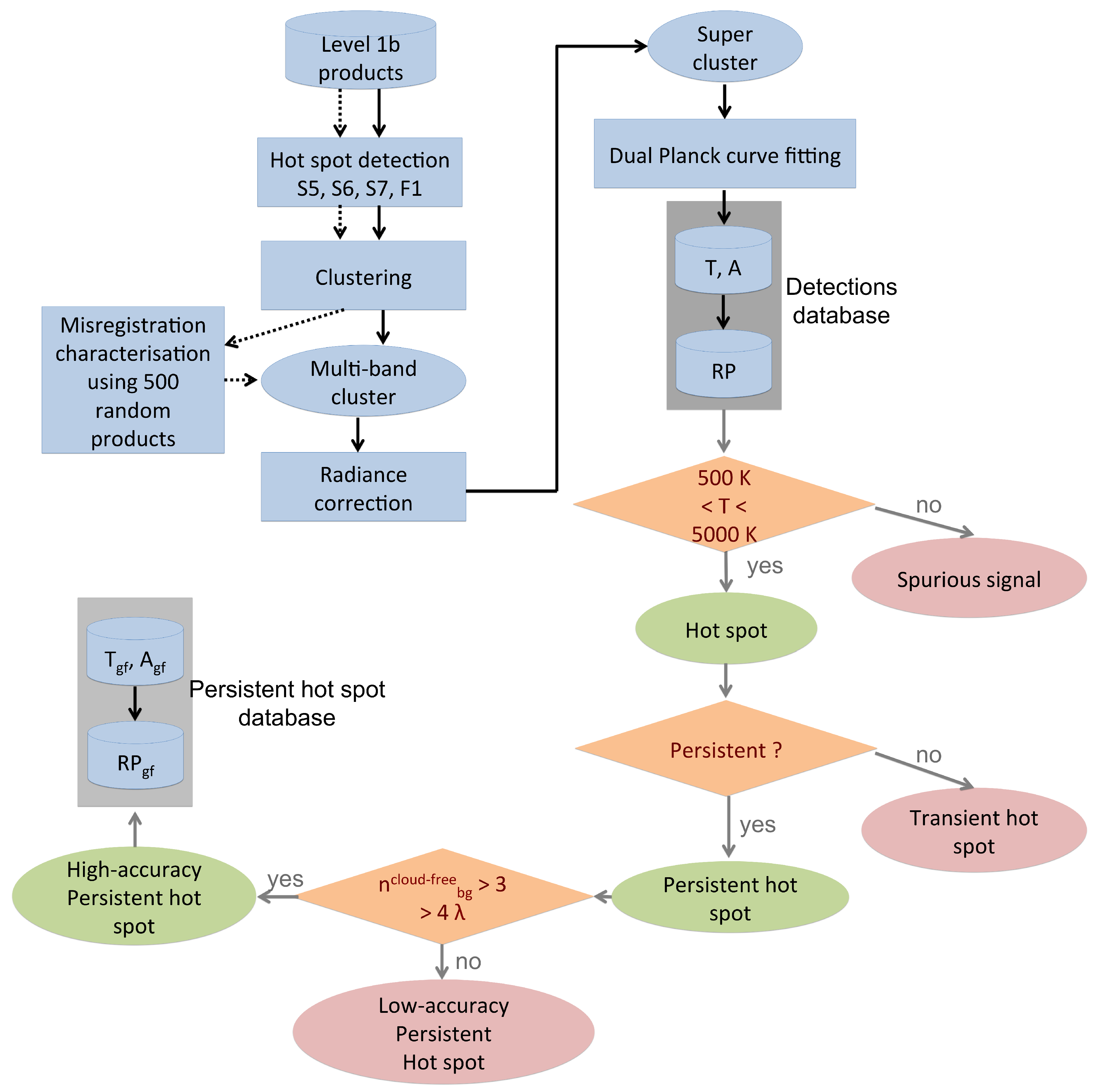
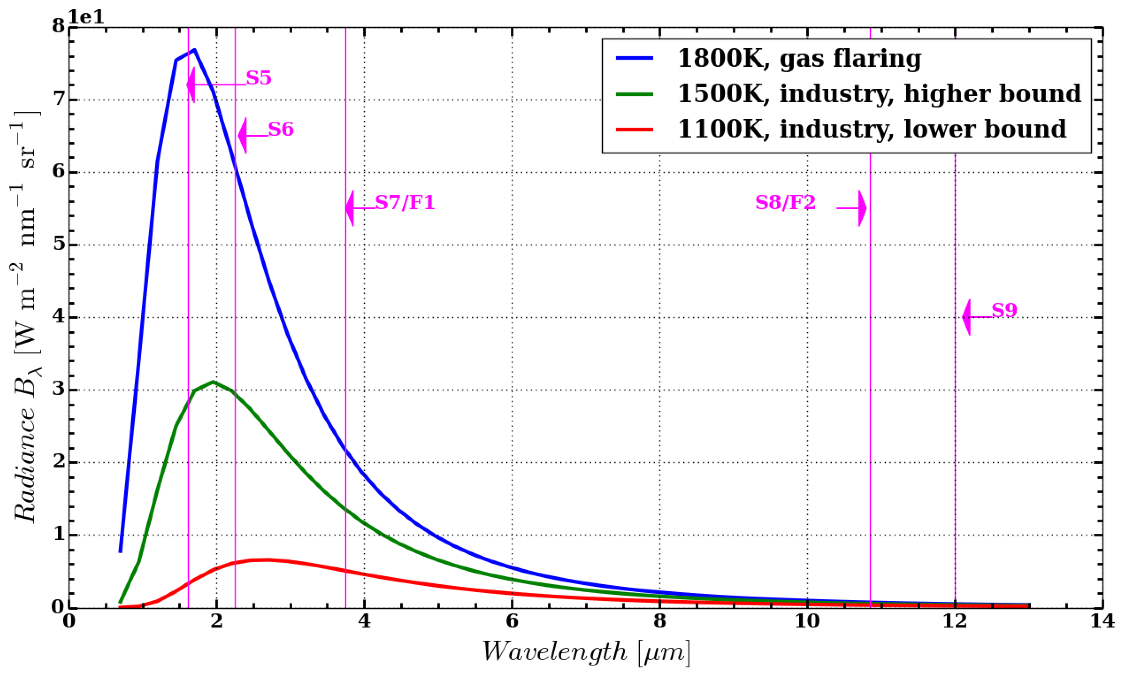
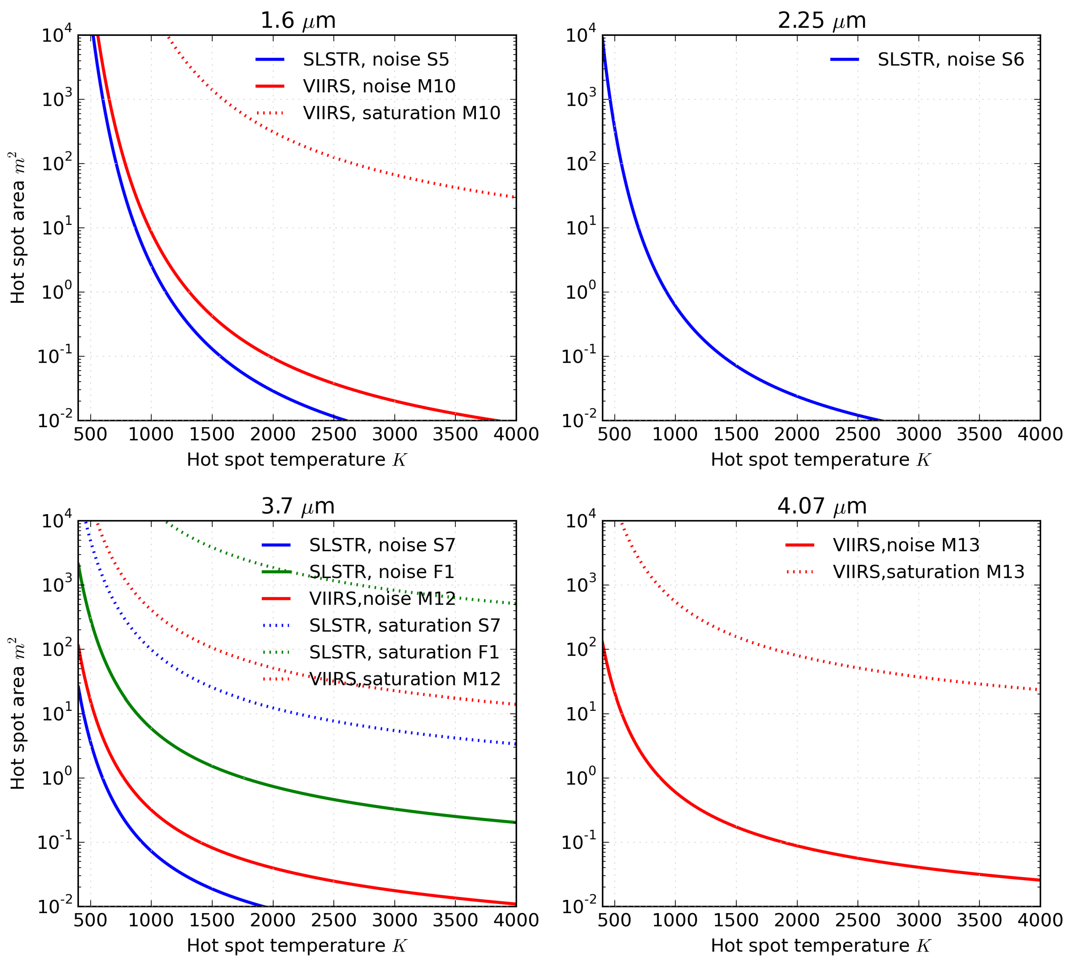
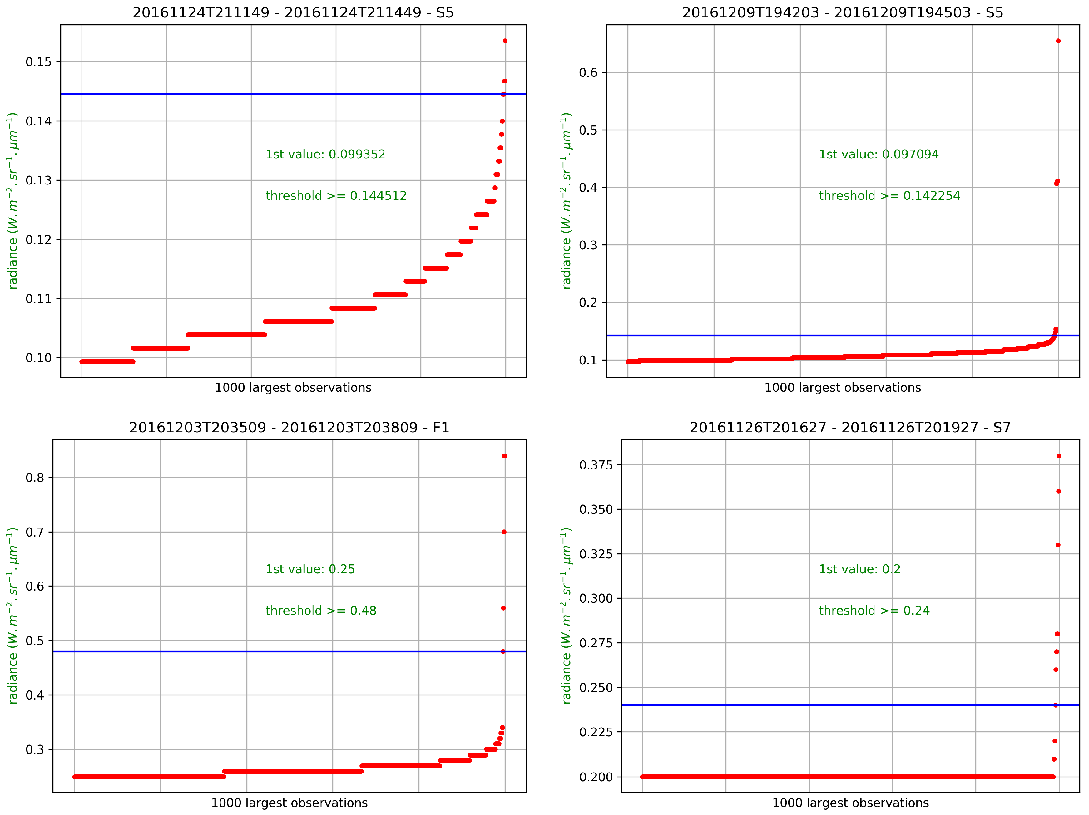
3.1. Detection
- The cut-off value was set as the lowest radiance which produced two statistically distinct groups (using the Mann-Whitney-Wilcoxon U-test). This approach failed to produce thresholds for the majority of products.
- The cut-off value was the lowest radiance which was not included within the confidence interval of the linear regression of the previous points. This methodology lead to the inclusion of irrealistically low radiance pixels as hot pixels and the subsequent production of extremely large clusters.
- Also based on the linear regression, we examined where the slope changed significantly and whether that point could be used as a threshold. This was highly dependent on the assumptions on the linear regression and considered as non robust.
- Otsu’s method [52] produced large thresholds and therefore left out real hot spots.
- An iterative clustering method which minimized differences between radiances of data points within two clusters also lead to large thresholds.
- Based on the fact that the night-time background is rather homogenous, the variance of the radiances of the product should be increased strongly by hot spots, while the background pixels should have a small variance. This approach was very sensitive on the a priori explained variance expected and was therefore abandoned.
- hot pixel location (, ) as pixel index pair
- radiance in W mm sr
- area in m (the the pixel length on the x and y axis is computed as average of the ground distance between the pixel and its direct neighbours in those axes).
3.2. Clustering
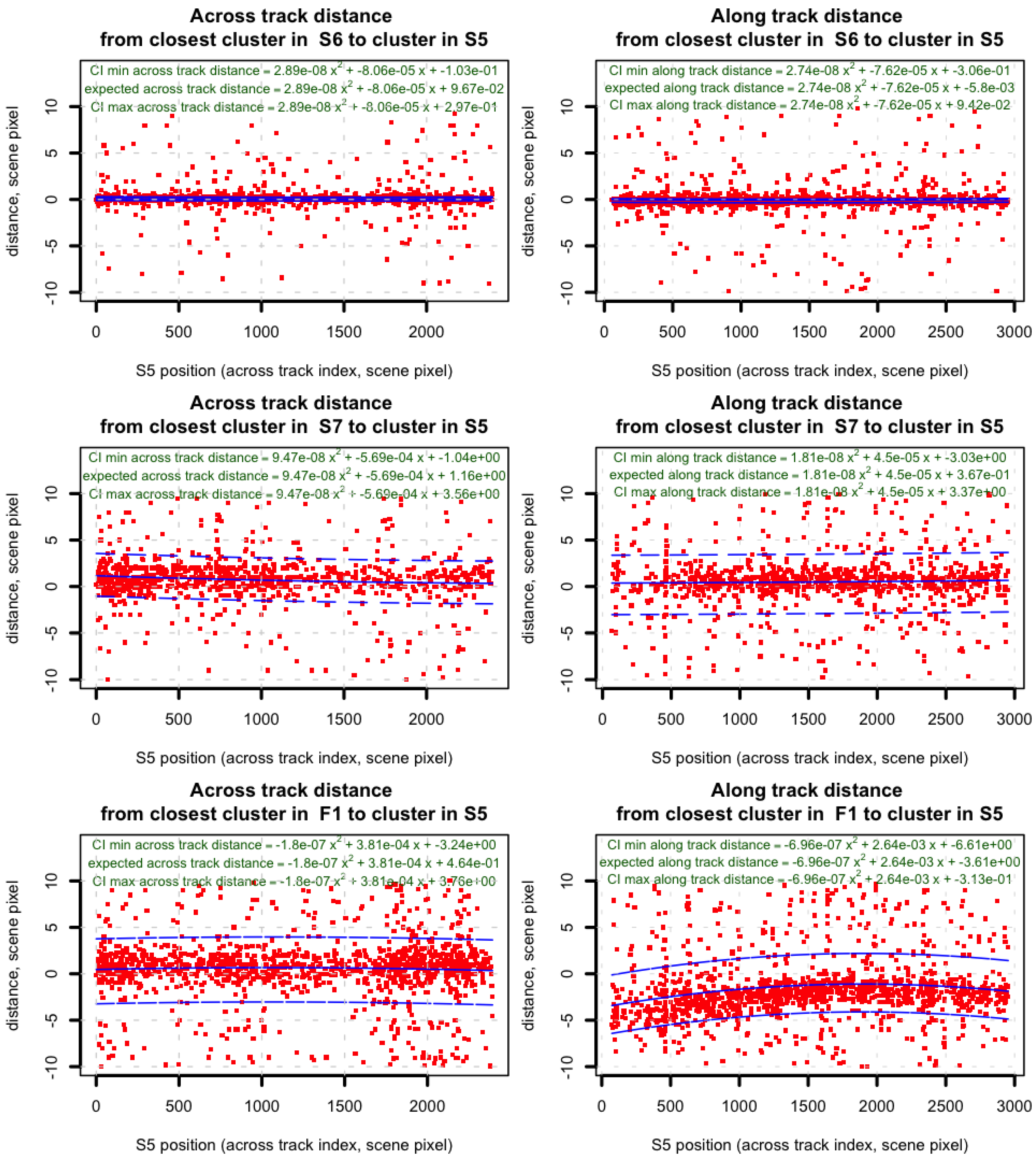
3.3. Misregistration Characterisation
3.4. Misregistration Correction: Building Multi-Band Clusters
3.5. Radiance Corrections
3.6. Super Cluster Definition
3.7. Planck Curve Fitting
3.8. Radiative Power
4. Results
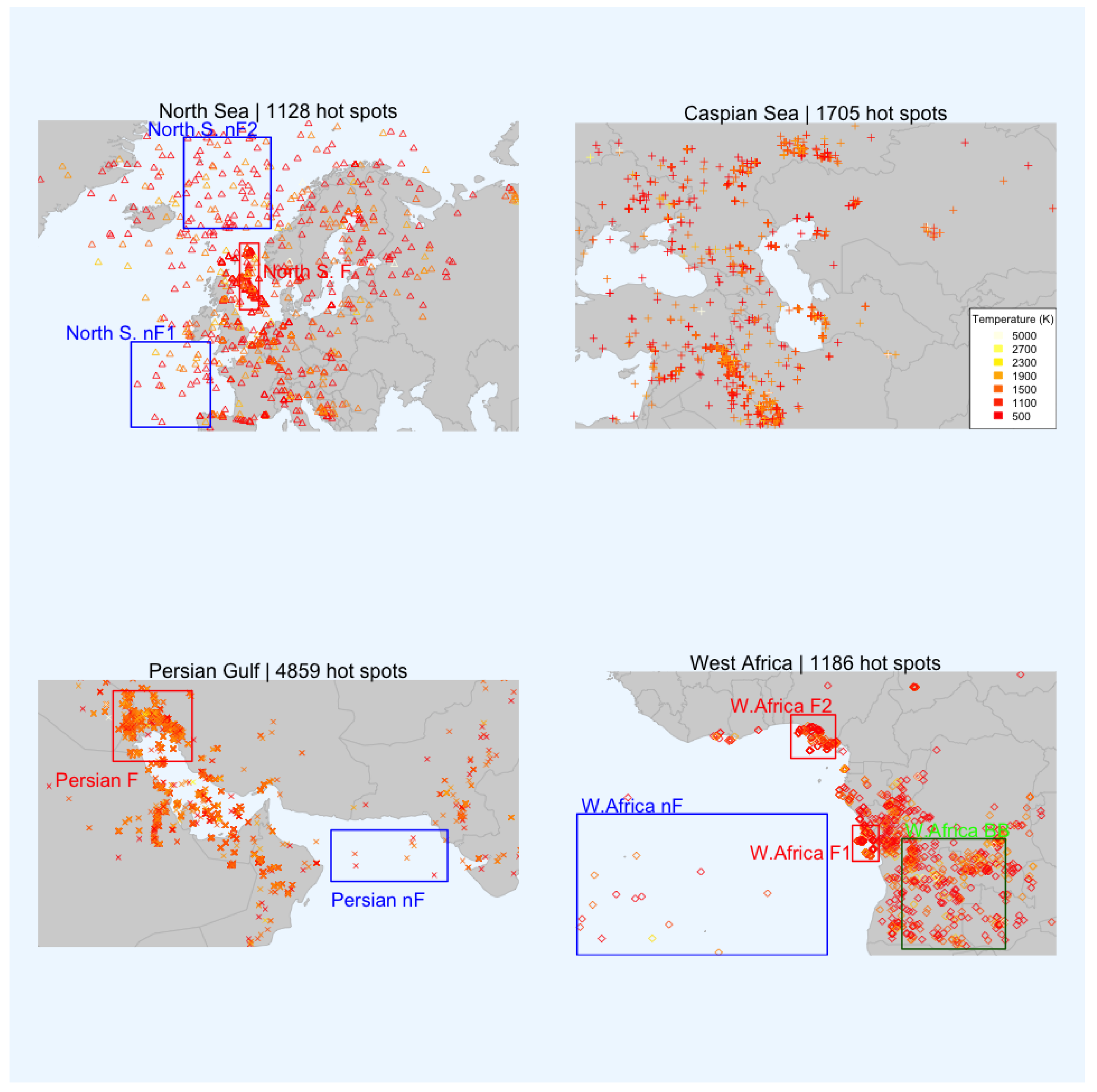
4.1. Regional Study: 4 Flaring Regions
4.1.1. Detection Thresholds
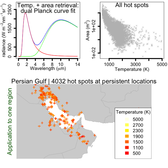
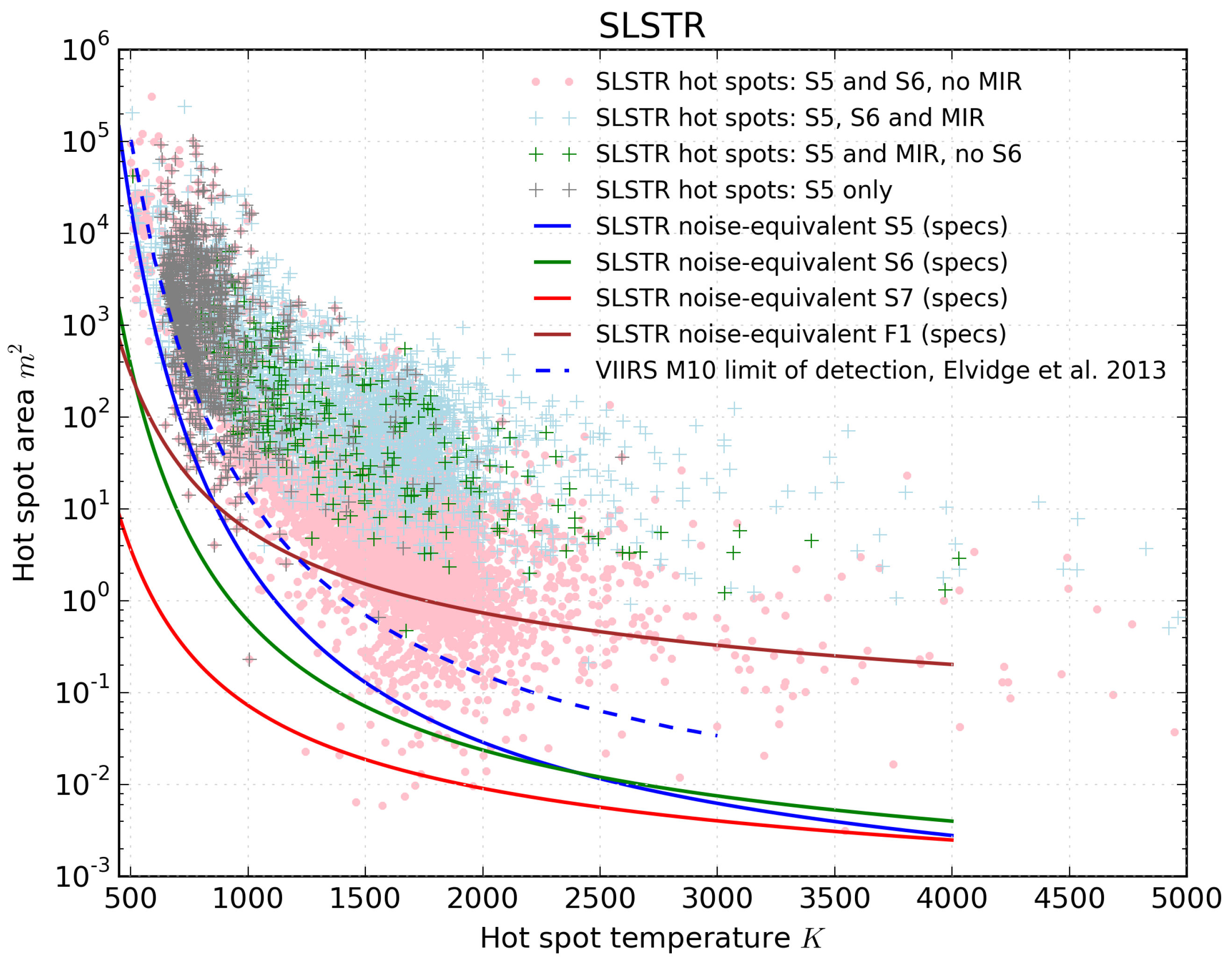
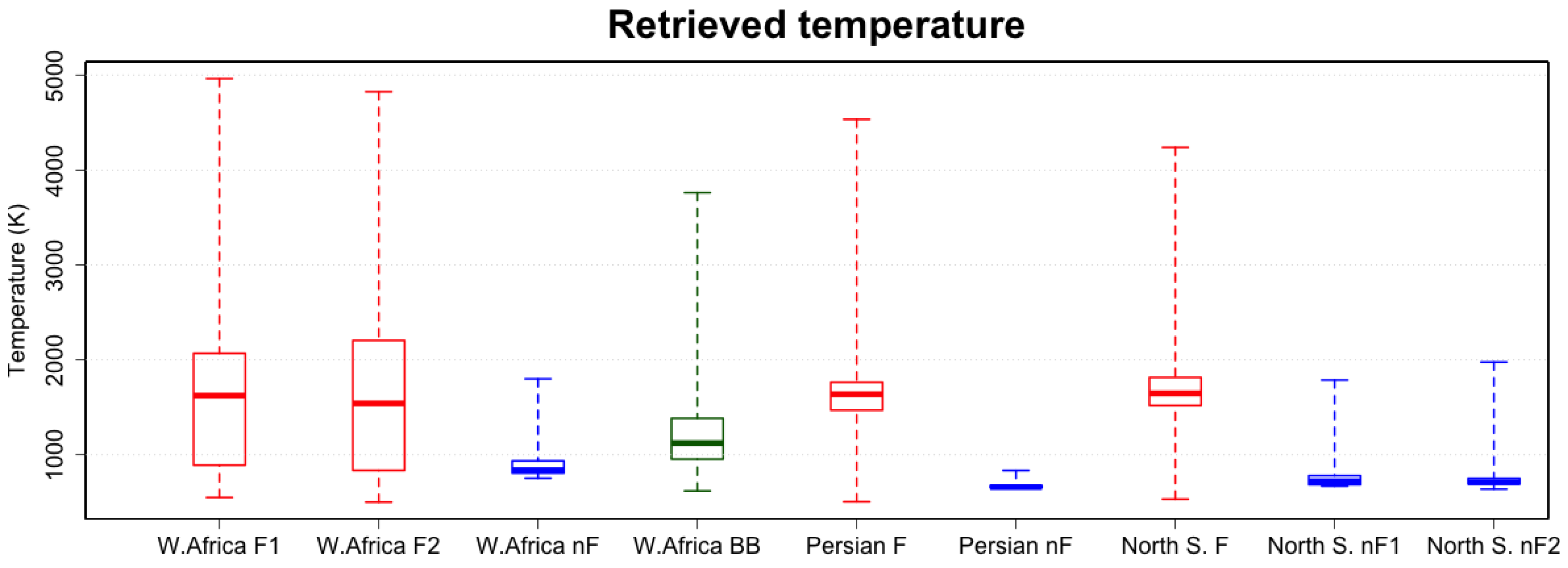
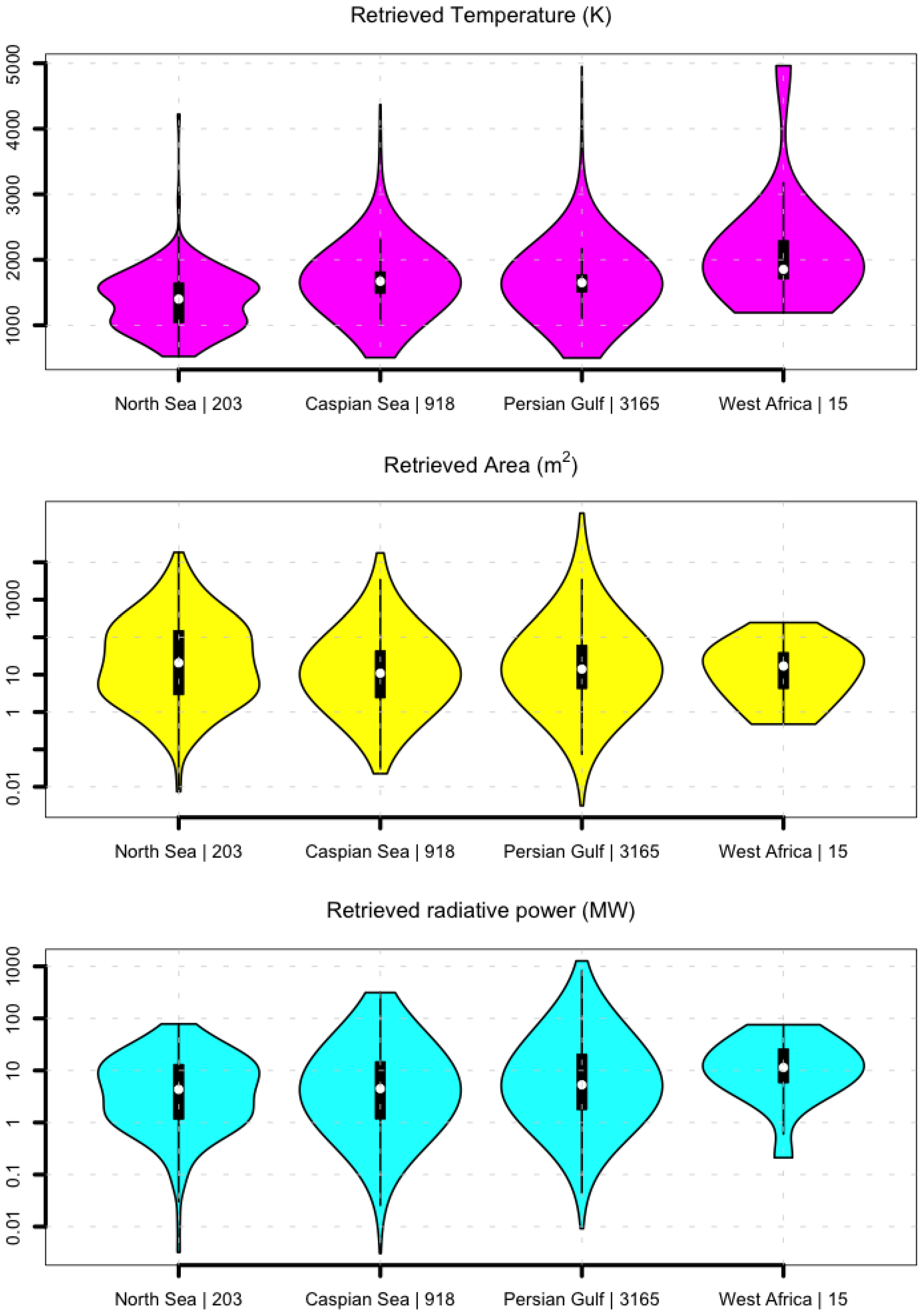
4.1.2. Temperature and Area Retrievals
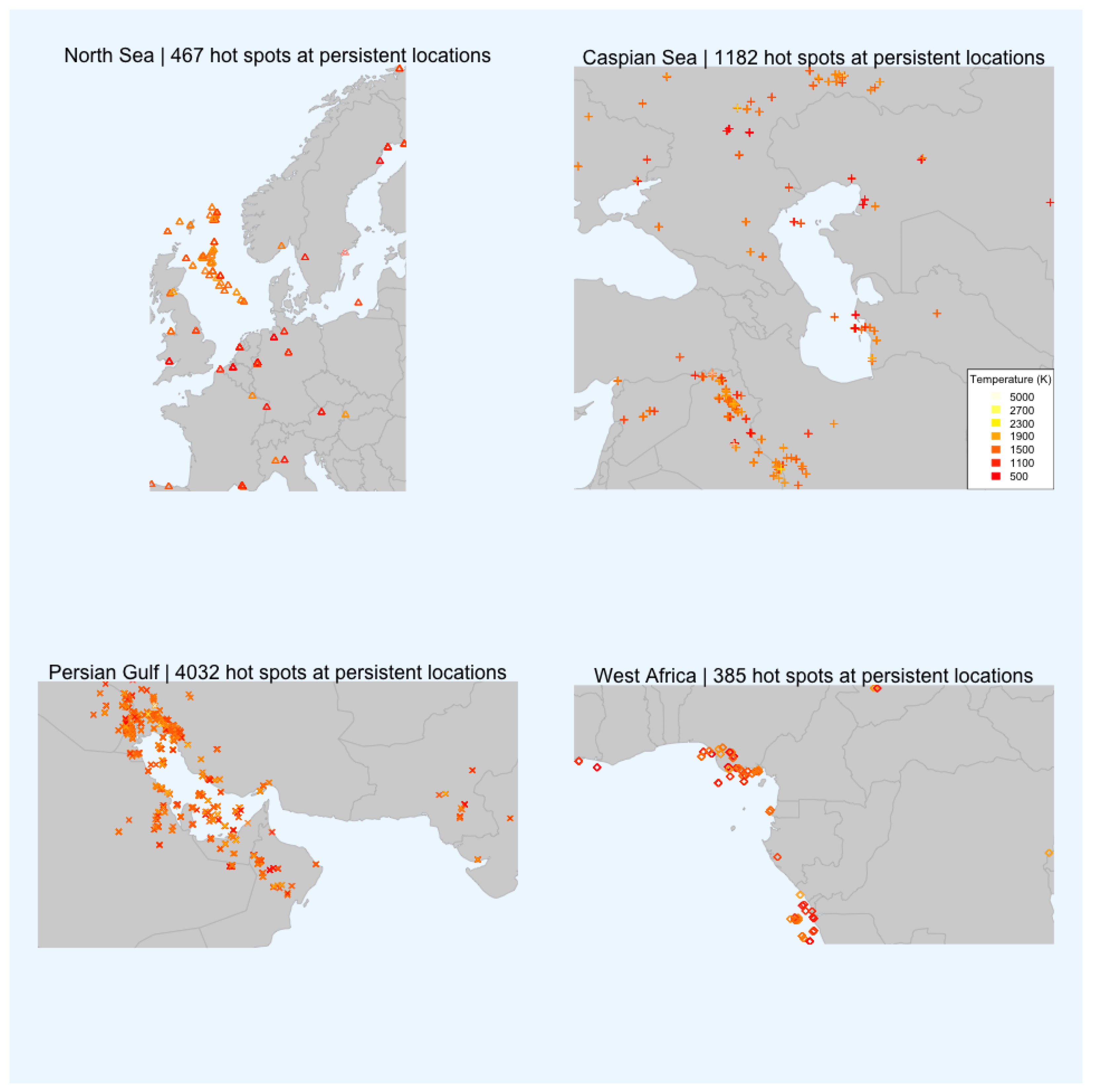
4.1.3. Persistence
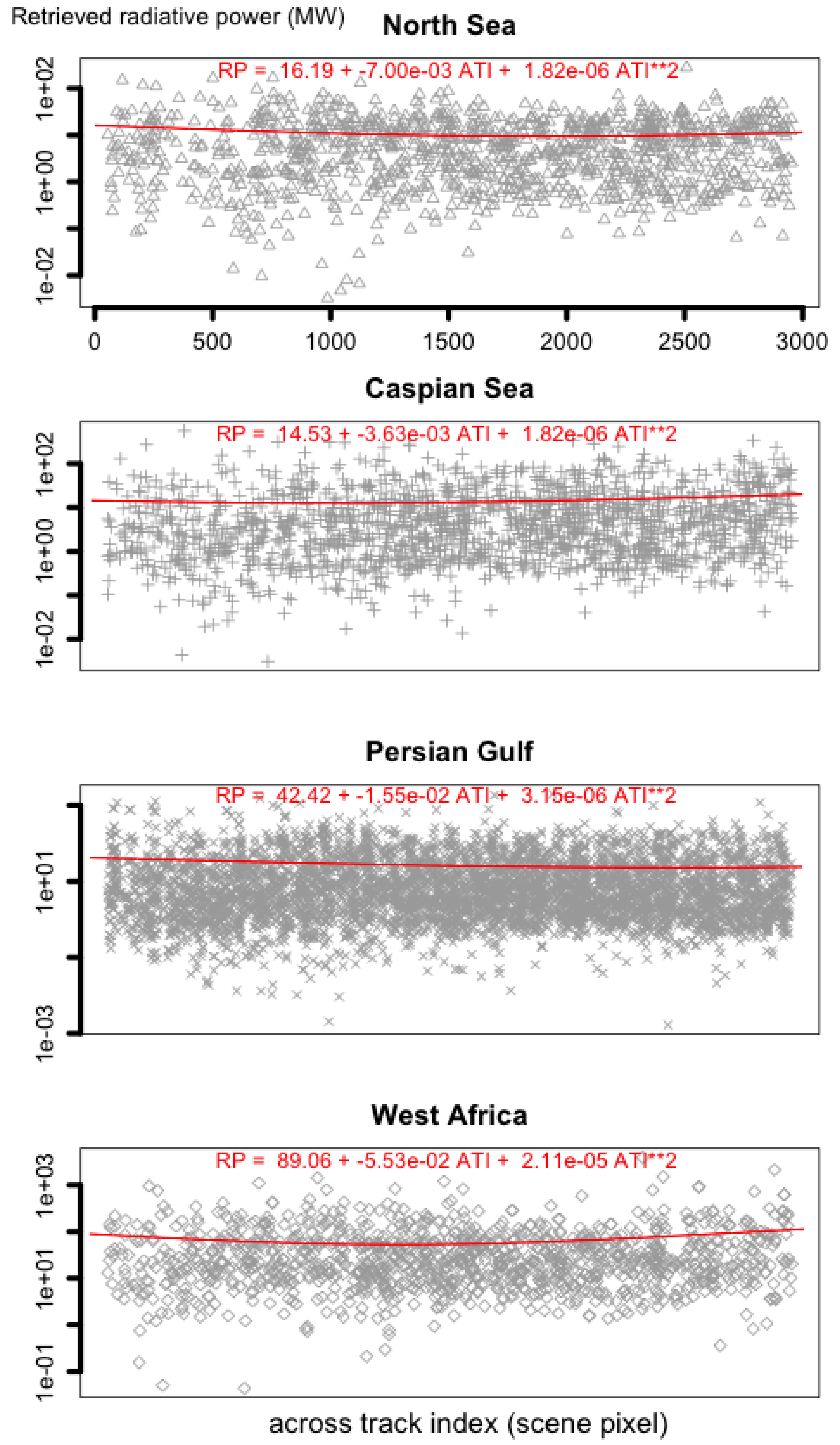
4.1.4. Selection of Persistent Hot Spots and Radiative Power Computations
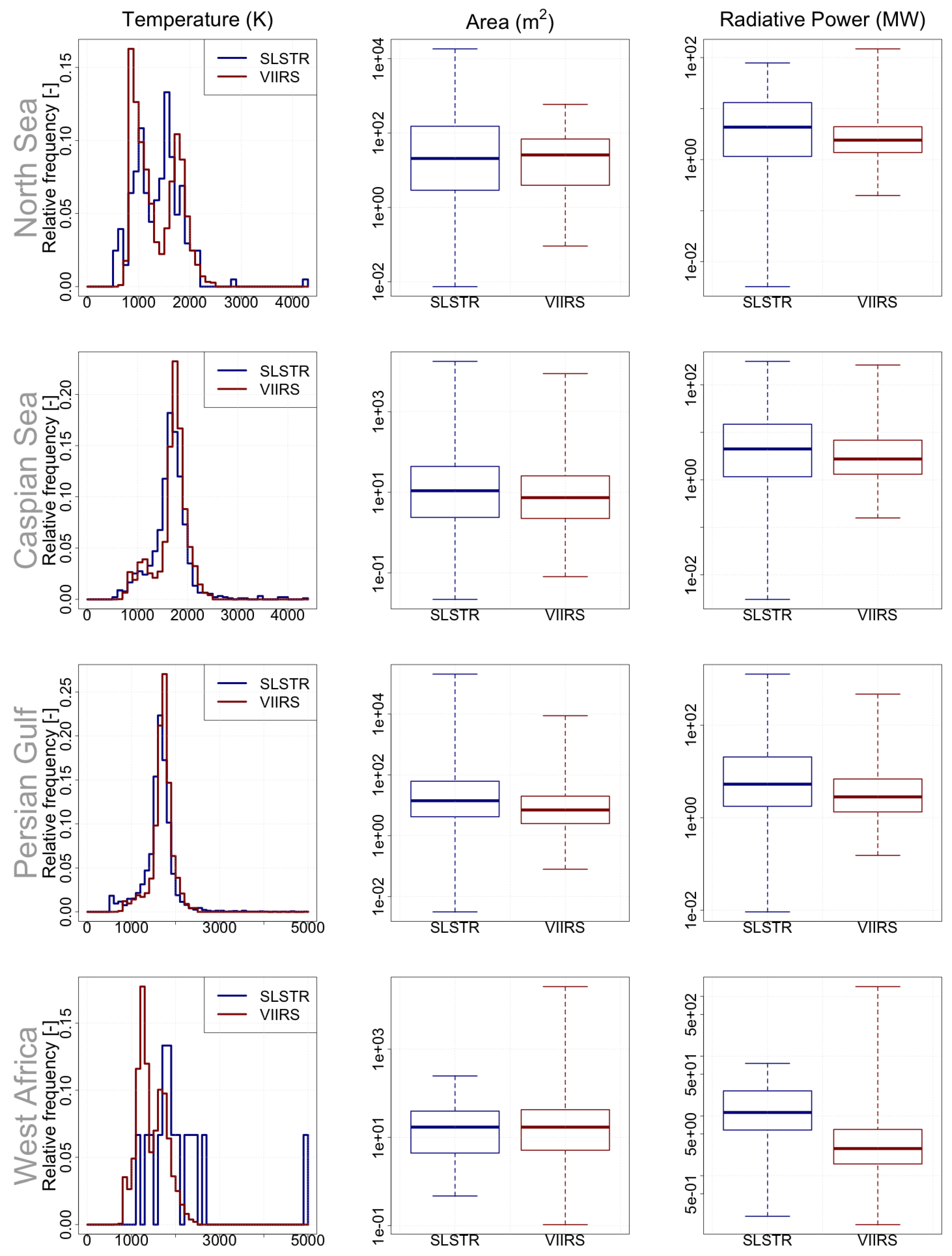
4.1.5. Comparison with VIIRS Nightfire
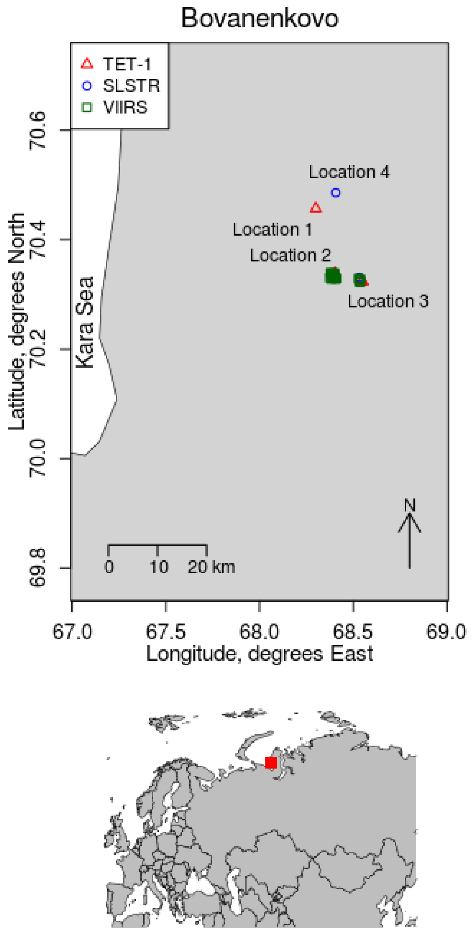
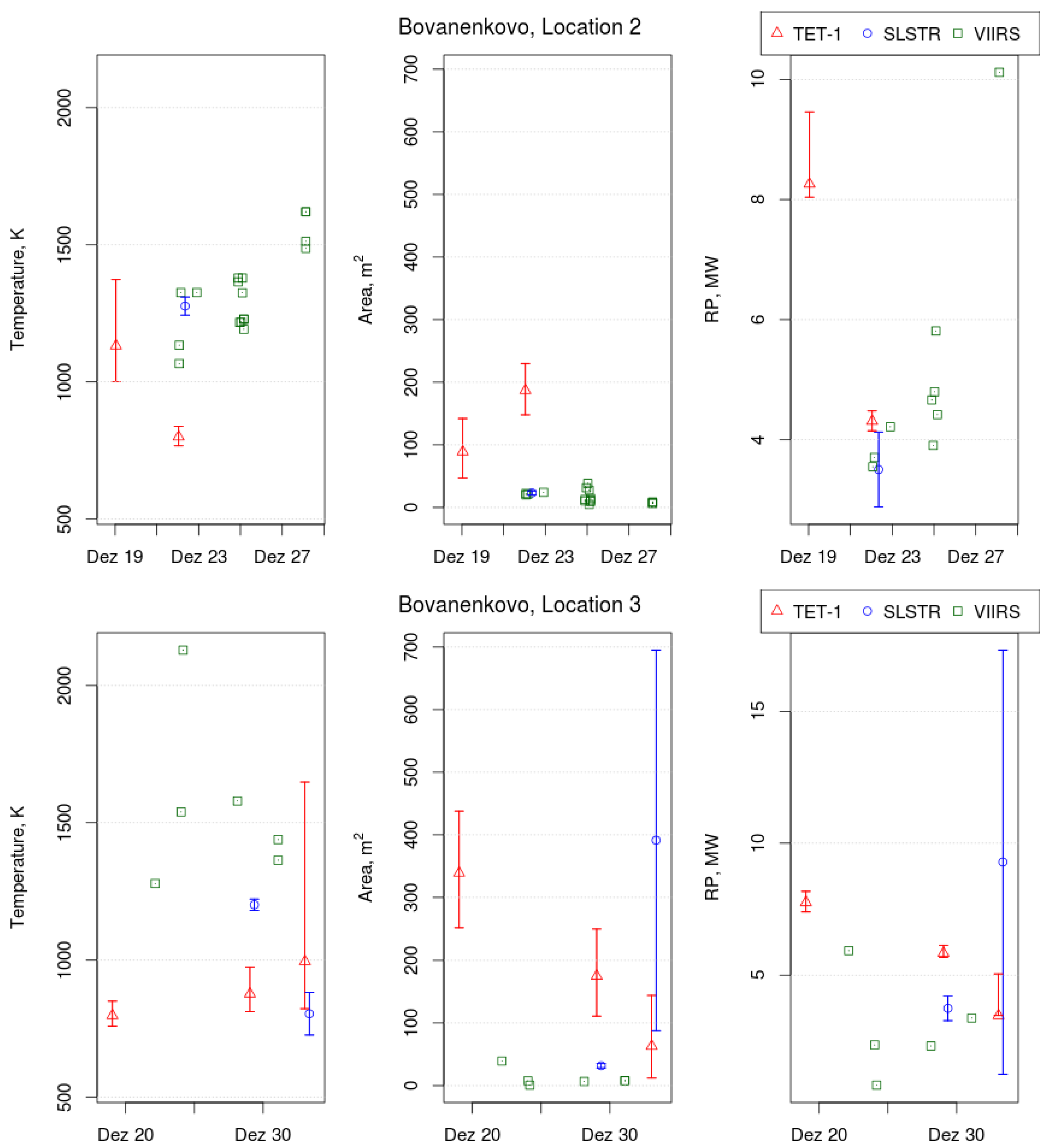
4.2. Single Site Study: Bovanenkovo, Yamal Peninsula
5. Conclusions
Supplementary Materials
Author Contributions
Funding
Acknowledgments
Conflicts of Interest
References
- Ismail, O.; Umukoro, G. Global Impact of Gas Flaring. Energy Power Eng. 2012, 4, 290–302. [Google Scholar] [CrossRef]
- Aghalino, S.O. Gas Flaring, Environmental Pollution and Abatement Measures in Nigeria, 1969–2001. J. Sustain. Dev. Afr. 2009, 11, 219–238. [Google Scholar]
- Nwoye, C.I.; Nwakpa, S.O.; Nwosu, I.E.; Odo, J.U.; Chinwuko, E.C.; Idenyi, N.E. Multi-Factorial Analysis of Atmospheric Noise Pollution Level Based on Emitted Carbon and Heat Radiation during Gas Flaring. J. Atmos. Pollut. 2014, 2, 22–29. [Google Scholar] [CrossRef]
- Anomohanran, O. Determination of greenhouse gas emission resulting from gas flaring activities in Nigeria. Energy Policy 2012, 45, 666–670. [Google Scholar] [CrossRef]
- Ajao, E.A.; Anurigwo, S. Land-Based Sources of Pollution in the Niger Delta, Nigeria. Ambio 2002, 13, 442–445. [Google Scholar] [CrossRef]
- Julius, O.O. Environmental impact of gas flaring within Umutu-Ebedei gas plant in Delta State, Nigeria. Arch. Appl. Sci. Res. 2011, 3, 272–279. [Google Scholar]
- Obioh, I.; Oluwole, A.F.; Akeredolu, F.A. Non-CO2 gaseous emissions from upstream oil and gas operations in Nigeria. Environ. Monit. Assess. 1994, 31, 67–72. [Google Scholar] [CrossRef] [PubMed]
- Uzomah, V.; Sangodoyin, A. Rainwater chemistry as influenced by atmospheric deposition of pollutants in Southern Nigeria. Environ. Manag. Health 2000, 11, 149–156. [Google Scholar] [CrossRef]
- Nwaichi, E.; Uzazobona, M. Estimation of the CO2 Level due to Gas Flaring in the Niger Delta. Res. J. Environ. Sci. 2011, 5, 565–572. [Google Scholar] [CrossRef]
- Onu, P.u.; Quan, X.; Ling, X. Acid rain: An analysis on the cause, impacts and abatement measures Niger Delta perspective, Nigeria. Int. J. Sci. Eng. Res. 2014, 5, 1214–1219. [Google Scholar]
- European Commission, Joint Research Centre (JRC)/Netherlands Environmental Assessment Agency (PBL). Emission Database for Global Atmospheric Research (EDGAR), Release EDGARv4.2 FT2012. 2016. Available online: http://edgar.jrc.ec.europa.eu/overview.php?v=42FT2012 (accessed on 29 June 2018).
- Stohl, A.; Klimont, Z.; Eckhardt, S.; Kupiainen, K.; Shevchenko, V.P.; Kopeikin, V.M.; Novigatsky, A.N. Black carbon in the Arctic: The underestimated role of gas flaring and residential combustion emissions. Atmos. Chem. Phys. 2013, 13, 8833–8855. [Google Scholar] [CrossRef]
- Huang, K.; Fu, J.S.; Prikhodko, V.Y.; Storey, J.M.; Romanov, A.; Hodson, E.L.; Cresko, J.; Morozova, I.; Ignatieva, Y.; Cabaniss, J. Russian anthropogenic black carbon: Emission reconstruction and Arctic black carbon simulation. J. Geophys. Res. Atmos. 2015, 120, 11306–11333. [Google Scholar] [CrossRef]
- Quinn, P.K.; Shaw, G.; Andrews, E.; Dutton, E.G.; Ruoho Airola, T.; Gong, S.L. Arctic haze: Current trends and knowledge gaps. Tellus B 2007, 59, 99–114. [Google Scholar] [CrossRef]
- Doherty, S.J.; Warren, S.G.; Grenfell, T.C.; Clarke, A.D.; Brandt, R.E. Light-absorbing impurities in Arctic snow. Atmos. Chem. Phys. 2010, 10, 11647–11680. [Google Scholar] [CrossRef]
- Serreze, M.C.; Barry, R.G. Processes and impacts of Arctic amplification: A research synthesis. Glob. Planet. Chang. 2011, 77, 85–96. [Google Scholar] [CrossRef]
- Walsh, J.E. Intensified warming of the Arctic: Causes and impacts on middle latitudes. Glob. Planet. Chang. 2014, 117, 52–63. [Google Scholar] [CrossRef]
- Li, C.; Hsu, N.C.; Sayer, A.M.; Krotkov, N.A.; Fu, J.S.; Lamsal, L.N.; Lee, J.; Tsay, S.C. Satellite observation of pollutant emissions from gas flaring activities near the Arctic. Atmos. Environ. 2016, 133, 1–11. [Google Scholar] [CrossRef]
- Elvidge, C.D.; Zhizhin, M.; Baugh, K.; Hsu, F.C.; Ghosh, T. Methods for Global Survey of Natural Gas Flaring from Visible Infrared Imaging Radiometer Suite Data. Energies 2016, 9, 14. [Google Scholar] [CrossRef]
- Weyant, C.L.; Shepson, P.B.; Subramanian, R.; Cambaliza, M.O.L.; Heimburger, A.; McCabe, D.; Baum, E.; Stirm, B.H.; Bond, T.C. Black Carbon Emissions from Associated Natural Gas Flaring. Environ. Sci. Technol. 2016, 50, 2075–2081. [Google Scholar] [CrossRef] [PubMed]
- Conrad, B.M.; Johnson, M.R. Field Measurements of Black Carbon Yields from Gas Flaring. Environ. Sci. Technol. 2017, 51, 1893–1900. [Google Scholar] [CrossRef] [PubMed]
- Klimont, Z.; Kupiainen, K.; Heyes, C.; Purohit, P.; Cofala, J.; Rafaj, P.; Borken Kleefeld, J.; Schöpp, W. Global anthropogenic emissions of particulate matter including black carbon. Atmos. Chem. Phys. 2017, 17, 8681–8723. [Google Scholar] [CrossRef]
- Anejionu, O.C.; Blackburn, G.A.; Whyatt, J.D. Detecting gas flares and estimating flaring volumes at individual flow stations using MODIS data. Remote Sens. Environ. 2015, 158, 81–94. [Google Scholar] [CrossRef]
- Zhang, X.; Scheving, B.; Shoghli, B.; Zygarlicke, C.; Wocken, C. Quantifying Gas Flaring CH4 Consumption Using VIIRS. Remote Sens. 2015, 7, 9529. [Google Scholar] [CrossRef]
- Croft, T. Burning waste gas in oil fields. Nature 1973, 245, 375–376. [Google Scholar] [CrossRef]
- Croft, T. Nighttime images of the earth from space. Sci. Am. 1978, 239, 86–98. [Google Scholar] [CrossRef]
- Elvidge, C.D.; Imhoff, M.L.; Baugh, K.E.; Hobson, V.R.; Nelson, I.; Safran, J.; Dietz, J.B.; Tuttle, B.T. Night-time lights of the world: 1994–1995. ISPRS J. Photogramm. Remote Sens. 2001, 56, 81–99. [Google Scholar] [CrossRef]
- Elvidge, C.D.; Baugh, K.E.; Tuttle, B.T.; Howard, A.T.; Pack, D.W.; Milesi, C.; Erwin, E.H. A Twelve Year Record of National and Global Gas Flaring Volumes Estimated Using Satellite Data; Technical Report; World Bank: Washington, DC, USA, 2007. [Google Scholar]
- Elvidge, C.D.; Ziskin, D.; Baugh, K.E.; Tuttle, B.T.; Ghosh, T.; Pack, D.W.; Erwin, E.H.; Zhizhin, M. A Fifteen Year Record of Global Natural Gas Flaring Derived from Satellite Data. Energies 2009, 2, 595–622. [Google Scholar] [CrossRef]
- Mota, B.W.; Pereira, J.M.C.; Oom, D.; Vasconcelos, M.J.P.; Schultz, M. Screening the ESA ATSR-2 World Fire Atlas (1997–2002). Atmos. Chem. Phys. 2006, 6, 1409–1424. [Google Scholar] [CrossRef]
- Oom, D.; Pereira, J. Exploratory spatial data analysis of global MODIS active fire data. Int. J. Appl. Earth Obs. Geoinf. 2013, 21, 326–340. [Google Scholar] [CrossRef]
- Elvidge, C.D.; Baugh, K.E.; Ziskin, D.; Anderson, S.; Ghosh, T. Estimation of Gas Flaring Volumes Using NASA MODIS Fire Detection Products; Technical Report; NOAA National Geophysical Data Center: Boulder, CO, USA, 2011.
- Faruolo, M.; Coviello, I.; Filizzola, C.; Lacava, T.; Pergola, N.; Tramutoli, V. A satellite-based analysis of the Val d’Agri Oil Center (southern Italy) gas flaring emissions. Nat. Hazards Earth Syst. Sci. 2014, 14, 2783–2793. [Google Scholar] [CrossRef]
- Casadio, S.; Arino, O.; Serpe, D. Gas flaring monitoring from space using the ATSR instrument series. Remote Sens. Environ. 2012, 116, 239–249. [Google Scholar] [CrossRef]
- Casadio, S.; Arino, O.; Minchella, A. Use of ATSR and SAR measurements for the monitoring and characterisation of night-time gas flaring from off-shore platforms: The North Sea test case. Remote Sens. Environ. 2012, 123, 175–186. [Google Scholar] [CrossRef]
- Elvidge, C.D.; Zhizhin, M.; Hsu, F.C.; Baugh, K.E. VIIRS Nightfire: Satellite Pyrometry at Night. Remote Sens. 2013, 5, 4423–4449. [Google Scholar] [CrossRef]
- Anejionu, O.C.D.; Blackburn, G.A.; Whyatt, J.D. Satellite survey of gas flares: Development and application of a Landsat-based technique in the Niger Delta. Int. J. Remote Sens. 2014, 35, 1900–1925. [Google Scholar] [CrossRef]
- Fisher, D.; Wooster, M.J. Shortwave IR Adaption of the Mid-Infrared Radiance Method of Fire Radiative Power (FRP) Retrieval for Assessing Industrial Gas Flaring Output. Remote Sens. 2018, 10, 305. [Google Scholar] [CrossRef]
- Dozier, J. A Method for Satellite Identification of Surface Temperature Fields of Subpixel Resolution. Remote Sens. Environ. 1981, 11, 221–229. [Google Scholar] [CrossRef]
- Brieß, K.; Bärwald, W.; Gill, E.; Kayal, H.; Montenbruck, O.; Montenegro, S.; Halle, W.; Skrbek, W.; Studemund, H.; Terzibaschian, T.; et al. Technology demonstration by the BIRD-mission. Acta Astronaut. 2005, 56, 57–63. [Google Scholar] [CrossRef]
- Walter, I.; Briess, K.; Baerwald, W.; Lorenz, E.; Skrbek, W.; Schrandt, F. A microsatellite platform for hot spot dedection. Acta Astronaut. 2005, 56, 221–229. [Google Scholar] [CrossRef]
- Zhukov, B.; Lorenz, E.; Oertel, D.; Wooster, M.; Roberts, G. Spaceborne detection and characterization of fires during the bi-spectral infrared detection (BIRD) experimental small satellite mission (2001–2004). Remote Sens. Environ. 2006, 100, 29–51. [Google Scholar] [CrossRef]
- Oertel, D.; Briess, K.; Lorenz, E.; Skrbek, W.; Zhukov, B. Detection, monitoring and quantitative analysis of wildfires with the BIRD satellite. In Remote Sensing for Agriculture, Ecosystems, and Hydrology V, Proceedings of SPIE, Barcelona, Spain, 8–12 September 2004; Owe, M., D’Urso, G., Moreno, J.F., Calera, A., Eds.; SPIE: Bellingham, WA, USA, 2004; Volume 5232, pp. 208–218. [Google Scholar] [CrossRef]
- Zhukov, B.; Briess, K.; Lorenz, E.; Oertel, D.; Skrbek, W. Detection and analysis of high-temperature events in the BIRD mission. Acta Astronaut. 2005, 56, 65–71. [Google Scholar] [CrossRef]
- Reile, H.; Lorenz, E.; Terzibaschian, T. The FireBird Mission—A Scientific Mission for Earth Observation and Hot Spot Detection. In Proceedings of the Small Satellites for Earth Observation Digest of the 9th International Symposium of the International Academy of Astronautics, Berlin, Germany, 8–12 April 2013. [Google Scholar]
- Coppo, P.; Ricciarelli, B.; Brandani, F.; Delderfield, J.; Ferlet, M.; Mutlow, C.; Munro, G.; Nightingale, T.; Smith, D.; Bianchi, S.; et al. SLSTR: A high accuracy dual scan temperature radiometer for sea and land surface monitoring from space. J. Mod. Opt. 2010, 57, 1815–1830. [Google Scholar] [CrossRef]
- Coppo, P.; Mastrandrea, C.; Stagi, M.; Calamai, L.; Barilli, M.; Nieke, J. The Sea and Land Surface Temperature Radiometer (SLSTR) Detection Assembly design and performance. In Proceedings of the SPIE, Dresden, Germany, 16 October 2013; Meynart, R., Neeck, S.P., Shimoda, H., Eds.; SPIE: Bellingham, WA, USA, 2013; Volume 8889. [Google Scholar] [CrossRef]
- Cao, C.; Xiong, J.; Blonski, S.; Liu, Q.; Uprety, S.; Shao, X.; Bai, Y.; Weng, F. Suomi NPP VIIRS sensor data record verification, validation, and long-term performance monitoring. J. Geophys. Res. Atmos. 2013, 118, 11664–11678. [Google Scholar] [CrossRef]
- Reed, R.J. North American Combustion Handbook Vol. I: Combustion, Fuels, Stoichiometry, Heat Transfer, Fluid Flow; North American Manufacturing Company: Cleveland, OH, USA, 1986. [Google Scholar]
- Leifer, I.; Lehr, W.J.; Simecek-Beatty, D.; Bradley, E.; Clark, R.; Dennison, P.; Hu, Y.; Matheson, S.; Jones, C.E.; Holt, B.; et al. State of the art satellite and airborne marine oil spill remote sensing: Application to the BP Deepwater Horizon oil spill. Remote Sens. Environ. 2012, 124, 185–209. [Google Scholar] [CrossRef]
- Hilbig, T.; Weber, M.; Bramstedt, K.; Noel, S.; Burrows, J.P.; Krijger, J.M.; Snel, R.; Meftah, M.; Dame, L.; Bekki, S.; et al. The new SCIAMACHY reference solar spectral irradiance and its validation. Sol. Phys. 2017. submitted. [Google Scholar]
- Otsu, N. A Threshold Selection Method from Gray-Level Histograms. IEEE Trans. Syst. Man Cybern. 1979, 9, 62–66. [Google Scholar] [CrossRef]
- Muirhead, K.; Cracknell, A.P. Identification of gas flares in the North Sea using satellite data. Int. J. Remote Sens. 1984, 5, 199–212. [Google Scholar] [CrossRef]
- Smith, D. Sentinel-3 SLSTR—Performance and Calibration. In Proceedings of the Sentinel-3 Validation Team Meeting, Darmstadt, Germany, 13–15 March 2018. [Google Scholar]
- Liu, Y.; Hu, C.; Zhan, W.; Sun, C.; Murch, B.; Ma, L. Identifying industrial heat sources using time-series of the VIIRS Nightfire product with an object-oriented approach. Remote Sens. Environ. 2018, 204, 347–365. [Google Scholar] [CrossRef]
- Johnson, M.; Kostiuk, L. Efficiencies of low-momentum jet diffusion flames in crosswinds. Combust. Flame 2000, 123, 189–200. [Google Scholar] [CrossRef]
- Leahey, D.; Preston, K.; Strosher, M. Theoretical and observational assessments of flare efficiencies. J. Air Waste Manag. Assoc. 2001, 51, 1610–1616. [Google Scholar] [CrossRef] [PubMed]
- Johnson, M.; Kostiuk, L. A parametric model for the efficiency of a flare in crosswind. Proc. Combust. Inst. 2002, 29, 1943–1950. [Google Scholar] [CrossRef]
- Ismail, O.S.; Umukoro, G.E. Modelling combustion reactions for gas flaring and its resulting emissions. J. King Saud Univ. Eng. Sci. 2016, 28, 130–140. [Google Scholar] [CrossRef]
- Pohl, J.H.; Tichenor, B.A.; Lee, J.; Payne, R. Combustion Efficiency of Flares. Combust. Sci. Technol. 1986, 50, 217–231. [Google Scholar] [CrossRef]
- Hollingsworth, A.; Engelen, R.J.; Benedetti, A.; Dethof, A.; Flemming, J.; Kaiser, J.W.; Morcrette, J.J.; Simmons, A.J.; Textor, C.; Boucher, O.; et al. Toward a Monitoring and Forecasting System for Atmospheric Composition: The GEMS Project. Bull. Am. Meteorol. Soc. 2008, 89, 1147–1164. [Google Scholar] [CrossRef]
- Stein, O.; Flemming, J.; Inness, A.; Kaiser, J.W.; Schultz, M.G. Global reactive gases forecasts and reanalysis in the MACC project. J. Integr. Environ. Sci. 2012, 9, 57–70. [Google Scholar] [CrossRef]
- Kaiser, J.W.; Heil, A.; Andreae, M.O.; Benedetti, A.; Chubarova, N.; Jones, L.; Morcrette, J.J.; Razinger, M.; Schultz, M.G.; Suttie, M.; et al. Biomass burning emissions estimated with a global fire assimilation system based on observed fire radiative power. Biogeosciences 2012, 9, 527–554. [Google Scholar] [CrossRef]


| HSRS on TET-1 | VIIRS on Suomi-NPP | SLSTR on Sentinel-3A | |
|---|---|---|---|
| Start of operation | 2013 | 2011 | 2016 |
| Orbit | Sun synchronous | Sun synchronous | Sun synchronous |
| altitude (km) | 445 | 834 | 814.5 |
| Vis-NIR bands (m) | DNB: 0.5–0.9 | ||
| M7: 0.85–0.89 | |||
| M8: 1.23–1.25 | |||
| SWIR bands | M10: 1.58–1.64 | S5: 1.58–1.65 | |
| (m) | S6: 2.23–2.28 | ||
| Infrared | MIR: 3.40–4.20 TIR: 8.50–9.30 | M12: 3.55–3.93 | S7, F1: 3.55–3.93 |
| bands | M13: 3.97–4.13 | S8: 10.40–11.30 | |
| (m) | M15: 10.26–11.26 | S9, F2: 11.50–12.50 | |
| Ground | IR-bands: 170 | M-bands: 750 | S4–S6: 500 |
| resolution (m) | S7–S9, F1–F2: 1000 | ||
| Swath (km) | IR: 178 | 3040 | 1420 |
| Sensor | Region | Sampling Dates | n | |
|---|---|---|---|---|
| Regional study | SLSTR | North Sea | 17 November–18 December 2016 | 189 |
| Caspian Sea | 17 November–20 December 2016 | 99 | ||
| Persian Gulf | 17 November–31 December 2016 | 153 | ||
| West Africa | 25 July–29 September 2016 | 364 | ||
| VIIRS (Nightfire) | Global | 2016 | 587 | |
| Single site study | SLSTR | Yamal peninsula | 15 December 2016 – 2 January 2017 | 43 |
| VIIRS (Nightfire) | 6 | |||
| HSRS | 12 |
| North Sea | Caspian Sea | Persian Gulf | West Africa | |
|---|---|---|---|---|
| SLSTR | ||||
| hot spots | 1128 | 1705 | 4859 | 1186 |
| persistent hot spots | 467 | 1182 | 4032 | 385 |
| high-accuracy persistent hot spots | 203 | 874 | 3096 | 15 |
| persistent locations | 72 | 148 | 359 | 57 |
| persistent locations detected by VIIRS | 71 | 148 | 359 | 57 |
| SLSTR | HSRS | VIIRS | Total | |
|---|---|---|---|---|
| Location 1 | 0 | 1 | 0 | 1 |
| Location 2 | 1 | 2 | 17 | 20 |
| Location 3 | 2 | 3 | 6 | 11 |
| Location 4 | 1 | 0 | 0 | 1 |
| Total | 4 | 6 | 23 | 33 |
© 2018 by the authors. Licensee MDPI, Basel, Switzerland. This article is an open access article distributed under the terms and conditions of the Creative Commons Attribution (CC BY) license (http://creativecommons.org/licenses/by/4.0/).
Share and Cite
Caseiro, A.; Rücker, G.; Tiemann, J.; Leimbach, D.; Lorenz, E.; Frauenberger, O.; Kaiser, J.W. Persistent Hot Spot Detection and Characterisation Using SLSTR. Remote Sens. 2018, 10, 1118. https://doi.org/10.3390/rs10071118
Caseiro A, Rücker G, Tiemann J, Leimbach D, Lorenz E, Frauenberger O, Kaiser JW. Persistent Hot Spot Detection and Characterisation Using SLSTR. Remote Sensing. 2018; 10(7):1118. https://doi.org/10.3390/rs10071118
Chicago/Turabian StyleCaseiro, Alexandre, Gernot Rücker, Joachim Tiemann, David Leimbach, Eckehard Lorenz, Olaf Frauenberger, and Johannes W. Kaiser. 2018. "Persistent Hot Spot Detection and Characterisation Using SLSTR" Remote Sensing 10, no. 7: 1118. https://doi.org/10.3390/rs10071118
APA StyleCaseiro, A., Rücker, G., Tiemann, J., Leimbach, D., Lorenz, E., Frauenberger, O., & Kaiser, J. W. (2018). Persistent Hot Spot Detection and Characterisation Using SLSTR. Remote Sensing, 10(7), 1118. https://doi.org/10.3390/rs10071118