Article

Very Deep Convolutional Neural Networks for Complex Land Cover Mapping Using Multispectral Remote Sensing Imagery

1
C-CORE and Department of Electrical Engineering, Memorial University of Newfoundland, St. John’s, NL A1B 3X5, Canada
2
CRC-Laboratory in Advanced Geomatics Image Processing, Department of Geodesy and Geomatics Engineering, University of New Brunswick, Fredericton, NB E3B 5A3, Canada
*
Author to whom correspondence should be addressed.
Remote Sens. 2018, 10(7), 1119; https://doi.org/10.3390/rs10071119
Submission received: 24 May 2018 / Revised: 30 June 2018 / Accepted: 12 July 2018 / Published: 14 July 2018

Abstract

:
Despite recent advances of deep Convolutional Neural Networks (CNNs) in various computer vision tasks, their potential for classification of multispectral remote sensing images has not been thoroughly explored. In particular, the applications of deep CNNs using optical remote sensing data have focused on the classification of very high-resolution aerial and satellite data, owing to the similarity of these data to the large datasets in computer vision. Accordingly, this study presents a detailed investigation of state-of-the-art deep learning tools for classification of complex wetland classes using multispectral RapidEye optical imagery. Specifically, we examine the capacity of seven well-known deep convnets, namely DenseNet121, InceptionV3, VGG16, VGG19, Xception, ResNet50, and InceptionResNetV2, for wetland mapping in Canada. In addition, the classification results obtained from deep CNNs are compared with those based on conventional machine learning tools, including Random Forest and Support Vector Machine, to further evaluate the efficiency of the former to classify wetlands. The results illustrate that the full-training of convnets using five spectral bands outperforms the other strategies for all convnets. InceptionResNetV2, ResNet50, and Xception are distinguished as the top three convnets, providing state-of-the-art classification accuracies of 96.17%, 94.81%, and 93.57%, respectively. The classification accuracies obtained using Support Vector Machine (SVM) and Random Forest (RF) are 74.89% and 76.08%, respectively, considerably inferior relative to CNNs. Importantly, InceptionResNetV2 is consistently found to be superior compared to all other convnets, suggesting the integration of Inception and ResNet modules is an efficient architecture for classifying complex remote sensing scenes such as wetlands.

Graphical Abstract

1. Introduction

Wetlands are transitional zones between terrestrial and aquatic systems that support a natural ecosystem of a variety of plant and animal species, adapted to wet conditions [1]. Flood- and storm-damage protection, water quality improvement and renovation, greenhouse gas reduction, shoreline stabilization, and aquatic productivity are only a handful of the advantages associated with wetlands. Unfortunately, wetlands have undergone variations due to natural processes, such as changes in temperature and precipitation caused by climate change, coastal plain subsidence and erosion, as well as human-induced disturbances such as industrial and residential development, agricultural activities, and runoff from lawns and farms [1].
Knowledge of the spatial distribution of these valuable ecosystems is crucial in order to characterize ecosystem processes and to monitor the subsequent changes over time [2]. However, the remoteness, vastness, and seasonally dynamic nature of most wetland ecosystems make conventional methods of data acquisition (e.g., surveying) labor-intensive and costly [3,4]. Fortunately, remote sensing, as a cost- and time-efficient tool, addresses the limitations of conventional techniques by providing valuable ecological data to characterize wetland ecosystems and to monitor land cover changes [5,6]. Optical remote sensing data have shown to be promising tools for wetland mapping and monitoring. This is because biomass concentration, leaf water content, and vegetation chlorophyll—all important characteristics of wetland vegetation—can be determined using optical satellite images [7]. In particular, optical remote sensing sensors collect spectral information of ground targets at various points of the electromagnetic spectrum, such as visible and infrared, which is of great benefit for wetland vegetation mapping [7]. Therefore, several studies reported the success of wetland mapping using optical satellite imagery [8,9,10,11].
Despite the latest advances in remote sensing tools, such as the availability of high spatial and temporal resolution satellite data and object-based image analysis tools [12], the classification accuracy of complex land cover, such as wetland ecosystems, is insufficient [5]. This could be attributed to the spectral similarity of wetland vegetation types, making the exclusive use of spectral information insufficient for the classification of heterogeneous land cover classes. In addition, several studies reported the significance of incorporating both spectral and spatial information for land cover mapping [1,13]. Thus, spatial features may augment spectral information and thereby contribute to the success of complex land cover mapping. Accordingly, several experiments were carried out to incorporate both spectral and spatial features into a classification scheme. These studies were based on the Markov Random Field (MRF) model [14], the Conditional Random Field (CRF) model [15], and Composite Kernel (CK) methods [16]. However, in most cases, the process of extracting a large number of features, the feature engineering process [17], for the purpose of supervised classification is time intensive, and requires broad and profound knowledge to extract amenable features. Furthermore, classification based on hand-crafted spatial features primarily relies on low-level features, resulting in insufficient classification results in most cases and a poor capacity for generalization [13].
Most recently, Deep Learning (DL), a state-of-the-art machine learning tool, has been placed in the spotlight in the field of computer vision and, subsequently, in remote sensing [18]. This is because these advanced machine learning algorithms address the primary limitations of the conventional shallow-structured machine learning tools, such as Support Vector Machine (SVM) and Random Forest (RF) [19]. Deep Belief Net (DBN) [20], Stacked Auto-Encoder (SAE) [21], and deep Convolutional Neural Network (CNN) [22,23] are current deep learning models, of which the latter is most well-known. Importantly, CNN has led to a series of breakthroughs in several remote sensing applications, such as classification [15], segmentation [24], and object detection [25], due to its superior performance in a variety of applications relative to shallow-structured machine learning tools. CNNs are characterized by multi-layered interconnected channels, with a high capacity for learning the features and classifiers from data spontaneously given their deep architecture, their capacity to adjust parameters jointly, and to classify simultaneously [26]. One of the ubiquitous characteristics of such a configuration is its potential to encode both spectral and spatial information into the classification scheme in a completely automated workflow [26]. Accordingly, the complicated, brittle, and multistage feature engineering procedure is replaced with a simple end-to-end deep learning workflow [17].
Notably, there is a different degree of abstraction for the data within multiple convolutional layers, wherein low-, mid-, and high-level information is extracted in a hierarchical learning framework at the initial, intermediate, and final layers, respectively [26]. This configuration omits the training process from scratch in several applications since the features in the initial layers are generic filters (e.g., edge) and, accordingly, are less dependent on the application. However, the latest layers are related to the final application and should be trained according to the given data and classification problem. This also addresses the poor generalization capacity of shallow-structured machine learning tools, which are site- and data-dependent, suggesting the versatility of CNNs [17].
Although the advent of CNN dates back to as early as the 1980s, when LeCun designed a primary convolutional neural network known as LeNet to classify handwritten digits, it gained recognition and was increasingly applied around 2010 [27]. This is attributable to the advent of more powerful hardware, larger datasets (e.g., ImageNet) [28], and new ideas, which consequently improved network architecture [23]. The original idea of deep CNNs [27] has been further developed by Krizhevsky and his colleagues, who designed a breakthrough CNN, known as AlexNet, a pioneer of modern deep CNNs, with multiple convolutional and max-pooling layers that provide deeper feature-learning at different spatial scales [22]. Subsequent successes have been achieved since 2014, when VGG [29], GoogLeNet (i.e., Inception network) [23], ResNet [30], and Xception [31] were introduced in the ImageNet Large-Scale Visual Recognition Challenge (ILSVRC).
The intricate tuning process, heavy computational burden, high tendency of overfitting, and the empirical nature of model establishment are the main limitations associated with deep CNNs [26]. Although some studies have argued that all deep learning methods have a black-box nature, it is not completely true for CNN [17]. This is because the features learned by CNNs can be visualized and, in particular, they are an illustration of visual concepts. There are three different strategies for employing current CNNs: A full-training network, a pre-trained network as a feature extractor, and fine-tuning of a pre-trained network. In the first case, a network is trained from scratch with random weights and biases to extract particular features for the dataset of interest. However, the limited number of training samples constrains the efficiency of this technique due to the overfitting problem. The other two strategies are more useful when a limited amount of training samples is available [26,32].
In cases of limited training data, a stacked auto-encoder (SAE) is also useful to learn the features from a given dataset using an unsupervised learning network [33]. In such a network, the deconstruction error between the input data at the encoding layer and its reconstruction at the decoding layer is minimized [34]. SAE networks are characterized by a relatively simple structure relative to deep CNNs and they have a great capacity for fast image interpretation. In particular, they convert raw data to an abstract representation using a simple non-linear model and they integrate features using an optimization algorithm. This results in a substantial decrease of redundant information between the features while achieving a strong generalization capacity [35].
Despite recent advances in deep CNNs, their applications in remote sensing have been substantially limited to the classification of very high spatial resolution aerial and satellite imagery from a limited number of well-known datasets, owing to the similar characteristics of these data to object recognition in computer vision. However, acquiring high spatial resolution imagery may be difficult, especially on a large scale. Accordingly, less research has been carried out on the classification of medium and high spatial resolution satellite imagery in different study areas. Furthermore, the capacity of CNNs has been primarily investigated for the classification of urban areas, whereas there is limited research examining the potential of state-of-the-art classification tools for complex land cover mapping. Complex land cover units, such as wetland vegetation, are characterized by high intra- and low inter-class variance, resulting in difficulties in their discrimination relative to typical land cover classes. Thus, an environment with such highly heterogeneous land cover is beneficial for evaluating the capacity of CNNs for the classification of remote sensing data. Finally, the minimal application of well-known deep CNNs in remote sensing may be due to the limitation of input bands. Specifically, these convnets are designed to work with three input bands (e.g., Red, Green, and Blue), making them inappropriate for most remote sensing data. This indicates the significance of developing a pipeline compatible with multi-channel satellite imagery.
The main goals of this study were, therefore, to: (1) Eliminate the limitation of the number of input bands by developing a pipeline in Python with the capacity to operate with multi-layer remote sensing imagery; (2) examine the power of deep CNNs for the classification of spectrally similar wetland classes; (3) investigate the generalization capacity of existing CNNs for the classification of multispectral satellite imagery (i.e., a different dataset than those they were trained for); (4) explore whether full-training or fine-tuning is the optimal strategy for exploiting the pre-existing convnets for wetland mapping; and (5) compare the efficiency of the most well-known deep CNNs, including DenseNet121, InceptionV3, VGG16, VGG19, Xception, ResNet50, and InceptionResNetV2, for wetland mapping in a comprehensive and elaborate analysis. Thus, this study contributes to the use of the state-of-the-art classification tools for complex land cover mapping using multispectral remote sensing data.

2. Materials and Methods

2.1. Deep Convolutional Neural Network

CNNs are constructed by multi-layer interconnected neural networks, wherein powerful low-, intermediate-, and high-level features are hierarchically extracted. A typical CNN framework has two main layers—the convolutional and pooling layers—that, together, are called the convolutional base of the network [17]. Some networks, such as AlexNet and VGG, also have fully connected layers. The convolutional layer has a filtering function and extracts spatial features from the images. Generally, the first convolutional layers extract low-level features or small local patterns, such as edges and corners, while the last convolutional layers extract high-level features, such as image structures. This suggests the high efficiency of CNNs for learning spatial hierarchical patterns. Convolutional layers are usually defined using two components: The convolution patch size (e.g., 3 × 3 or 5 × 5) and the depth of the output feature map, which is the number of filters (e.g., 32 filters). In particular, a rectangular sliding window with a fixed-size and a pre-defined stride is employed to produce convoluted feature maps using a dot product between the weights of the kernel and a small region of the input volume (i.e., the receptive field). A stride is defined as a distance between two consecutive convolutional windows. A stride of one is usually applied in convolutional layers since larger stride values result in down-sampling in feature maps [17]. A feature map is a new image generated by this simple convolution operation and is a visual illustration of the extracted features. Given the weight-sharing property of CNNs, the number of parameters is significantly reduced compared to fully connected layer, since all the neurons across a particular feature map share the same parameters (i.e., weights and biases).
A non-linearity function, such as the Rectified Linear Unit (ReLU) [36], is usually applied as an elementwise nonlinear activation function to each component in the feature map. The ReLU function is advantageous relative to conventional activation functions used in traditional neural networks, such as the hyperbolic tangent or sigmoid functions, for adding non-linearity to the network [36]. The ReLU significantly accelerates the training phase relative to the conventional functions with gradient descent. This is because of the so-called vanishing gradient problem, wherein the derivatives of earlier functions (e.g., sigmoid) are extremely low in the saturating region and, accordingly, the updates for the weights nearly vanish.
Due to the presence of common pixels in each window, several feature maps may be produced that are very similar, suggesting redundant information. Therefore, pooling layers are used after each convolutional layer to decrease the variance of the extracted features using simple operations such as the maximizing or averaging operations. The max- and average-pooling layers determine the maximum and mean values, respectively, using a fixed-size sliding window and a pre-defined stride over the feature maps and, thereby, are conceptually similar to the convolutional layer. In contrast to convolutional layers, a stride of two or larger is applied in the pooling layers to down-sample the feature maps. Notably, the pooling layer, or the sub-sampling layer, generalizes the output of the convolutional layer into a higher level and selects the more robust and abstract features for the next layers. Thus, the pooling layer decreases computational complexity during the training stage by shrinking the feature maps.
As mentioned, some networks may have fully connected layers before the classifier layer that connect the output of several stacked convolutional and pooling layers to the classifier layer. Overfitting may arise in the fully connected layer because it occupies a large number of parameters. Thus, the dropout technique, an efficient regularization technique, is useful to mitigate or decrease problems associated with overfitting. During training, this technique randomly drops some neurons and their connections across the network, which prevents neurons from excess co-adaptation and contributes to developing more meaningful independent features [22]. The last layer is a classification layer, which determines the posterior probabilities for each category. A softmax classifier, also known as a normalized exponential, is the most commonly used classifier layer among the deep learning community in the image field. Stochastic Gradient Descent (SGD) optimization in a backpropagation workflow is usually used to train CNNs and to compute adjusting weights. This is an end-to-end learning process, from the raw data (i.e., original pixels) to the final label, using a deep CNN.

2.1.1. VGG

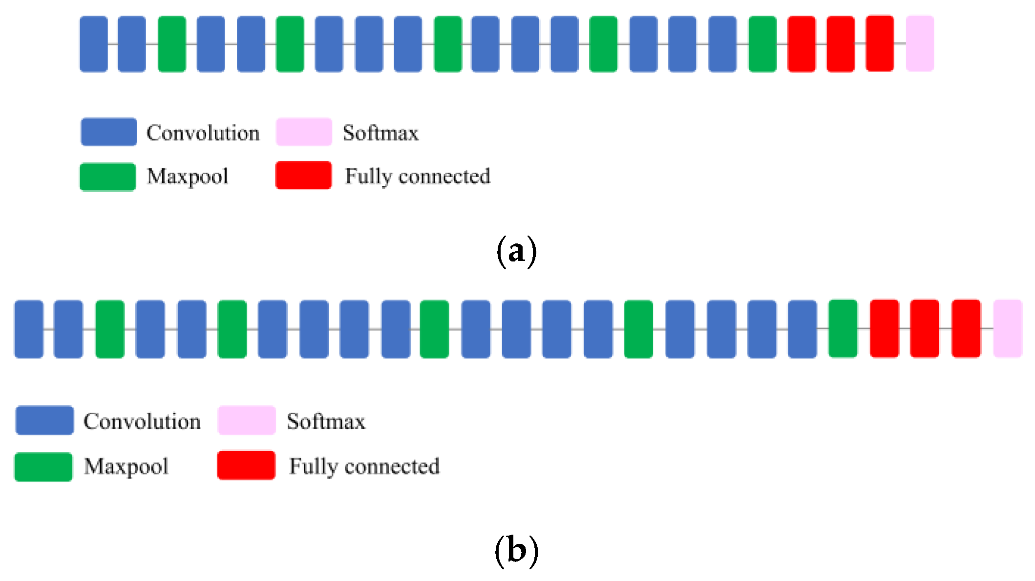
VGG network [29], the runner-up of the localization and classification tracks of the ILSVRC-2014 competition, is characterized by a deep network structure with a small convolutional filter of 3 × 3 compared to its predecessor, AlexNet [22]. VGG-VD group introduced six deep CNNs in the competition, among which two of them were more successful than the others, namely VGG16 and VGG19. The VGG16 consists of 13 convolutional layers and three fully connected layers, while the VGG19 has 16 convolutional layers and three fully connected layers. Both networks use a stack of small convolutional filters of 3 × 3 with stride 1, which are followed by multiple non-linearity layers (see Figure 1). This increases the depth of the network and contributes to learning more complex features. The impressive results of VGG revealed that the network depth is an important factor in obtaining high classification accuracy [32].

2.1.2. Inception

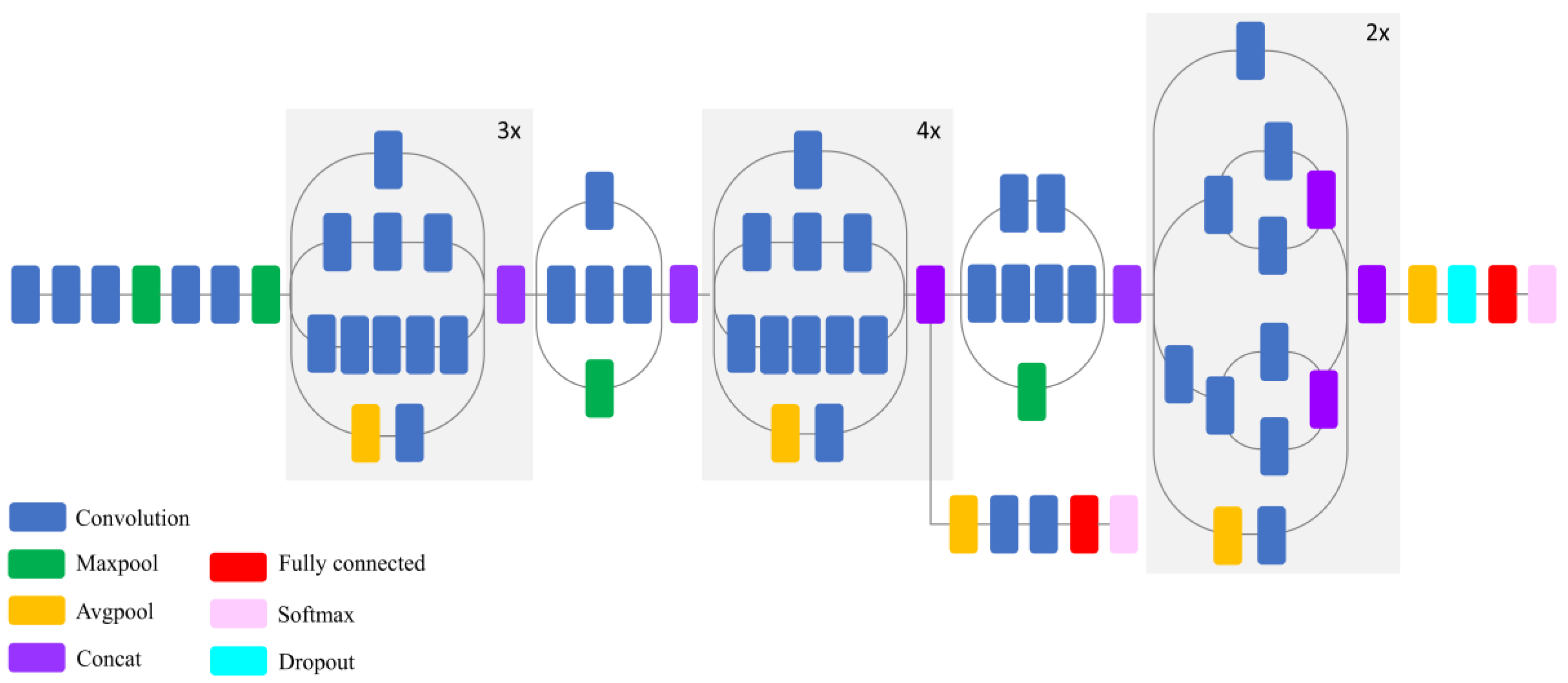
GoogLeNet, the winner of the classification and detection tracks of the ILSVRC-2014 competition, is among the first generation of non-sequential CNNs. In this network, both depth (i.e., the number of levels) and width (i.e., the number of units at each level), were increased without causing computational strain [23]. GoogLeNet is developed based on the idea that several connections between layers are ineffective and have redundant information due to the correlation between them. Accordingly, it uses an “Inception module”, a sparse CNN, with 22 layers in a parallel processing workflow, and benefits from several auxiliary classifiers within the intermediate layers to improve the discrimination capacity in the lower layers. In contrast to conventional CNNs such as AlexNet and VGG, wherein either a convolutional or a pooling operation can be used at each level, the Inception module could benefit from both at each layer. Furthermore, filters (convolutions) with varying sizes are used at the same layer, providing more detailed information and extracting patterns with different sizes. Importantly, a 1 × 1 convolutional layer, the so-called bottleneck layer, was employed to decrease both the computational complexity and the number of parameters. To be more precise, 1 × 1 convolutional layers were used just before a larger kernel convolutional filter (e.g., 3 × 3 and 5 × 5 convolutional layers) to decrease the number of parameters to be determined at each level (i.e., the pooling feature process). In addition, 1 × 1 convolutional layers make the network deeper and add more non-linearity by using ReLU after each 1 × 1 convolutional layer. In this network, the fully connected layers are replaced with an average pooling layer. This significantly decreases the number of parameters since the fully connected layers include a large number of parameters. Thus, this network is able to learn deeper representations of features with fewer parameters relative to AlexNet while it is much faster than VGG [31]. Figure 2 illustrates a compressed view of InceptionV3 employed in this study.

2.1.3. ResNet

ResNet, the winner of the classification task in the ILSVRC-2015 competition, is characterized by a very deep network with 152 layers [30]. However, the main problems associated with the deep network are difficulty in training, high training error, and the vanishing gradient that causes learning to be negligible at the initial layers in the backpropagation step. The deep ResNet configuration addresses the vanishing gradient problem by employing a deep residual learning module via additive identity transformations. Specifically, the residual module uses a direct path between the input and output and each stacked layer fits a residual mapping rather than directly fitting a desired underlying mapping [30]. Notably, the optimization is much easier on the residual map relative to the original, unreferenced map. Similar to VGG, 3 × 3 filters were mostly employed in this network; however, ResNet has fewer filters and less complexity relative to the VGG network [30]. Figure 3 illustrates a compressed view of ResNet, which was used in this study.

2.1.4. Xception

Xception network is similar to inception (GoogLeNet), wherein the inception module has been substituted with depth-wise separable convolutional layers [31]. Specifically, Xception’s architecture is constructed based on a linear stack of a depth-wise separable convolution layer (i.e., 36 convolutional layers) with linear residual connections (see Figure 4). There are two important convolutional layers in this configuration: A depth-wise convolutional layer [37], where a spatial convolution is carried out independently in each channel of input data, and a pointwise convolutional layer, where a 1 × 1 convolutional layer maps the output channels to a new channel space using a depth-wise convolution.

2.1.5. InceptionResNetV2

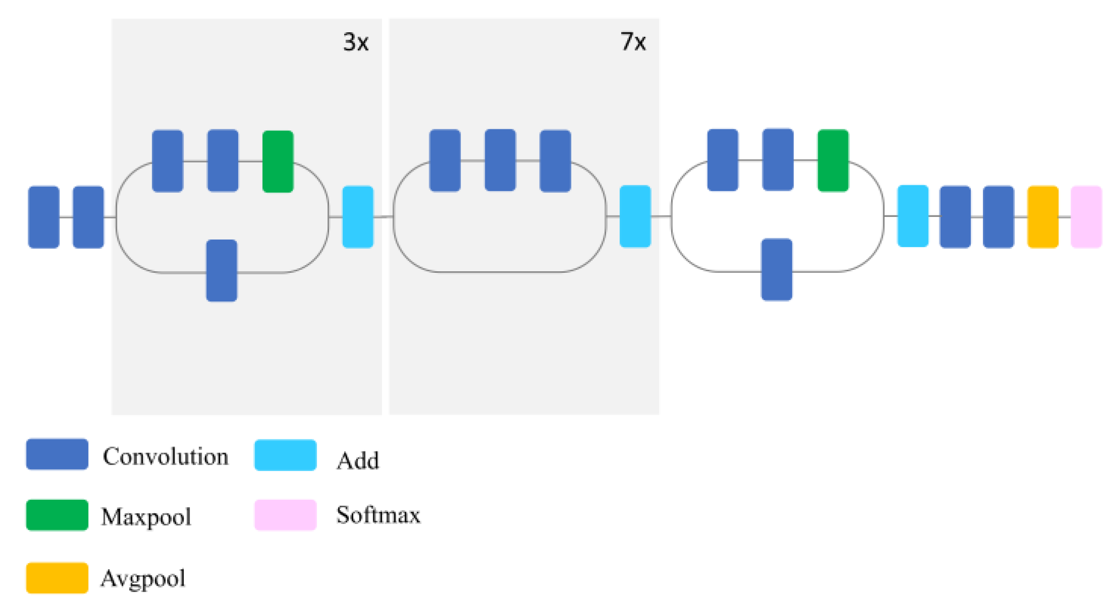
This network is constructed by integrating the two most successful deep CNNs, ResNet [30] and Inception [23], wherein batch-normalization is used only on top of the traditional layers, rather than on top of the summations. In particular, the residual modules are employed in order to allow an increase in the number of Inception blocks and, accordingly, an increase in network depth. As mentioned earlier, the most pronounced problem associated with very deep networks is the training phase, which can be addressed using the residual connections [30]. The network scales down the residual as an efficient approach to address the training problem when a large number of filters (greater than 1,000 filters) is used in the network. Specifically, the residual variants experience instabilities and the network cannot be trained when the number of filters exceeds 1,000. Therefore, scaling the residual contributes to stabilizing network training [38]. Figure 5 illustrates a compressed view of InceptionResNetV2 used in this study.

2.1.6. DenseNet

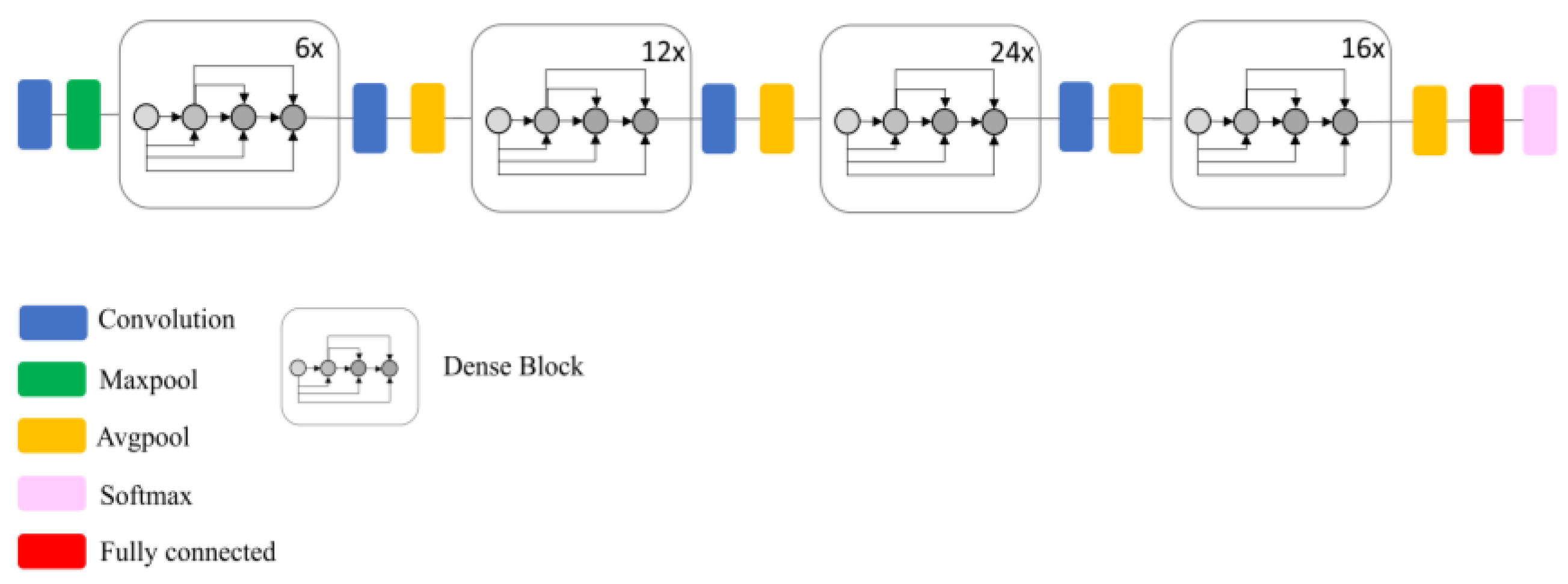
This network is also designed to address the vanishing gradient problem arising from the network depth. Specifically, all layers’ connection architectures are employed to ensure maximum flow of information between layers [39]. In this configuration, each layer acquires inputs from all previous layers and conveys its own feature-maps to all subsequent layers. The feature maps are concatenated at each layer to pass information from preceding layers to the subsequent layers. This network architecture removes the necessity to learn redundant information and accordingly, the number of parameters is significantly reduced (i.e., parameter efficiency). It is also efficient for preserving information owing to its all layers connection property. Huang et al. (2017) reported that the network performed very well for classifications with a small training data set and the overfitting is not a problem when DenseNet121 is employed [39]. Figure 6 illustrates a compressed view of DenseNet employed in this study.

2.2. Training

2.2.1. Fine-Tuning of a Pre-Trained Network

Fine-tuning of a pre-trained network is an optimal solution when a limited number of training samples are available. In this case, a fine adjustment is performed on the parameters of the top layers in a pre-trained network, while the first layers, representing general features, are frozen. Freezing is when weights for a layer or a set of layers are not updated during the training stage. Importantly, this approach benefits from the parameters learned from a network that has been previously trained using a specific dataset and, subsequently, adjusts the parameters for the dataset of interest. Accordingly, fine-tuning adjusts the parameters of the reused model, making it more relevant to the dataset of interest. Fine-tuning can be performed for either all layers or the top layers of a pre-trained network; however, the latter approach is preferred [17]. This is because the first layers in convnets encode generic, reusable features, whereas the last layers encode more specific features. Thus, it is more efficient to fine-tune those specific features. Furthermore, fine-tuning of all layers causes overfitting due to the large number of parameters, which should be determined during this process [17]. As such, in this study, fine-tuning of pre-existing convnets was carried out only on the top three layers. These may be either the fully connected layers alone (e.g., VGG) or both the fully connected and convolutional layers (e.g., Xception). Accordingly, the fine-tuning of the top three layers allowed us to compare the efficiency of fine-tuning for both fully connected and convolutional layers.
Notably, the number of input bands for these CNNs is limited to three because they have been trained using the ImageNet dataset; however, RapidEye imagery has five bands. Therefore, a band selection technique was pursued to determine three uncorrelated bands of RapidEye imagery most appropriate for use in CNNs. The results of this analysis demonstrated that green, red, and near-infrared bands contain the least redundant information and thus, they were selected for fine-tuning of CNNs in this study.

2.2.2. Full-Training

Full-training is feasible when a large number of training samples is available to aid in converging the network [26]. In this case, there is a full control on the network parameters and, additionally, more relevant features are produced since the network is specifically tuned with the dataset of interest. However, the full-training of a network from scratch is challenging due to computational and data strains, leading to overfitting problems. Some techniques, such as dropout layers and data augmentation and normalization, are useful for mitigating the problems that arise from overfitting. In particular, data augmentation, introduced by Krizhevsky in 2012, is a process that produces more training samples from existing training data using a number of random transformations (e.g., image translation and horizontal reflection) [22]. The main goal is that the model will never look at the same image twice. In particular, the model explores more aspects of the data, which contributes to a better generalization [17].
Notably, there are two different categories in the case of full-training of convnets. In the first category, a new CNN architecture is fully designed and trained from scratch. In this case, the number of convolutional, and pooling layers, neurons, the type of activation function, the learning rate, and the number of iterations should be determined. Conversely, the second strategy benefits from a pre-existing architecture and full-training is only employed using a given dataset. In the latter case, the network architecture and the number of parameters remain unchanged.
In this study, the second strategy was employed. In particular, we examined the potential of a number of pre-existing networks (e.g., VGG, Inception, and etc.,) for classification of complex land cover when they are trained from scratch using a new dataset substantially different from those (e.g., ImageNet) for which it was originally trained. Notably, full-training was employed for both three and five bands of RapidEye imagery. The full-training of three bands was performed to make the results comparable with those of the fine-tuning strategy.

2.3. Study Area and Satellite Data

The study area is located in the northeast portion of the Avalon Peninsula, Newfoundland and Labrador, Canada. Figure 7 shows the geographic location of the study area.
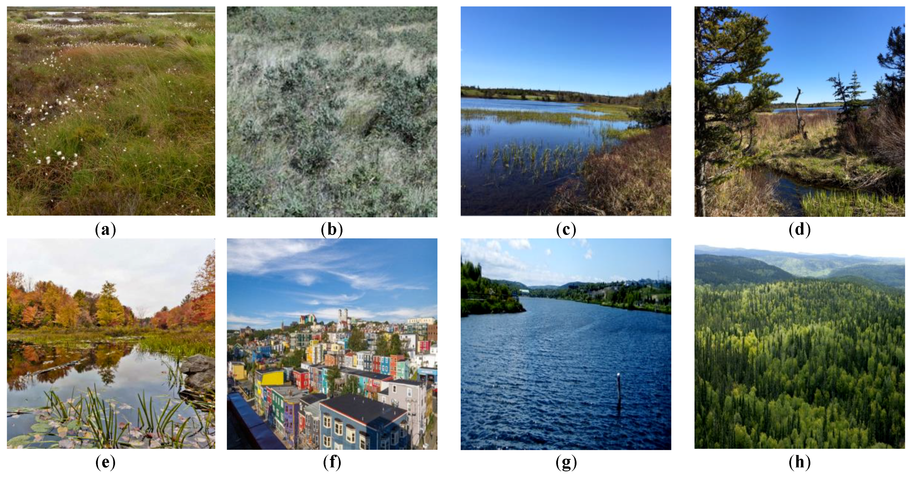
Land cover in the study area comprises a wide variety of wetland classes categorized by the Canadian Wetland Classification System (CWCS), including bog, fen, marsh, swamp, and shallow water [1]. Wetlands are characterized as complex species with high intra-class variance and low inter-class variance. Additionally, these classes are extremely different from typical objects found in the ImageNet dataset. Such a diverse ecological ecosystem is an ideal setting in which the efficiency and robustness of the state-of-the-art classification algorithms in a comprehensive and comparative study may be examined. Other land-cover classes found in the study area include urban, upland, and deep water classes. Figure 8 illustrates ground photo examples of land cover classes in this study.
Two level 3A multispectral RapidEye images with a spatial resolution of five meters, acquired on 18 June and 22 October 2015, were used for classification in this study. This imagery has five spectral bands, namely blue (440–510 nm), green (520–590 nm), red (630–685 nm), red edge (690–730 nm), and near-infrared (760–850 nm).

2.4. Training, Validation, and Testing Data

Field data were acquired for 257 ground sites in the summer and fall of 2015, 2016, and 2017 by collecting Global Positioning System (GPS) points at each site. For reference data preparation, polygons were sorted by size and alternately assigned to testing and training groups. This resulted in both the testing and training groups containing equal numbers of small and large wetland polygons to allow for similar pixel counts and to account for the high variation of intra-wetland size.
Importantly, five tiles of RapidEye optical images were mosaicked to cover the whole study region. The training polygons within the red rectangle (i.e., one RapidEye tile; see Figure 7), the so-called test-zone, were removed for the training of deep CNNs. In particular, all patches within the test-zone were only used for testing (i.e., accuracy assessment) of CNNs. Of the training sample data, 80% and 20% were used for training and validation, respectively. Notably, both training and validation were carried out using the first RapidEye image (18 June, 2015); however, the testing was applied only to the second RapidEye image (22 October, 2015), within the test-zone (see Figure 7, the red rectangle), to perform the robust classification accuracy assessment.
Accordingly, the training and testing samples were obtained from independent polygons from distinct geographic regions using satellite imagery acquired at different times. This procedure prevents information leaking from the testing dataset to the model by employing two spatially and geographically independent samples for training and testing.

2.5. Experiment Setup

A multispectral satellite image in three dimensions is represented as m × n × h, a 3D tensor, where m and n indicate the height and width of the image, respectively, and h corresponds to the number of channels. On the other hand, convnets require a 3D tensor as input and, accordingly, a patch-based labeling method was used in this study because it inherently aligns with CNNs. Using this approach, the multispectral image was decomposed into patches, which have both spectral and spatial information for a given pixel, and a class label is assigned to the center of each patch [40].
An optimal patch size was determined using a trial-and-error procedure, by taking into account a spatial resolution of 5 m for the input image and the contextual relationship of the objects [41]. In particular, different patch sizes of 5, 10, 15, 20, 25, 30, 35, and 40 were examined, and the patch size of 30 was found to be the optimal value that extracts local spatial correlation within a given neighborhood and contains sufficient information to generate a specific distribution for each object in the image. Thus, we obtained 3D tensors with dimensions of either 30 × 30 × 5 (when using 5 multispectral bands) or 30 × 30 × 3 (when using 3 multispectral bands), which have both spatial and spectral information at a given location.
In the patch-based CNN, a particular class label is assigned to the given patch when a small rectangle in the center of that patch completely covers a single object [42]. In this study, the training polygons were not rectangular, causing challenges during labeling when a patch contains more than one class.Accordingly, within a given patch size of 30 × 30, if an 8 × 8 rectangle covered only a single class (e.g., bog), then the label of this patch was assigned to that class (bog). Conversely, when this small rectangular window covered more than one class (e.g., both bog and fen), this patch was removed and excluded from further processing. Thus, the selected patches for the training of convnets covered more than 50% of the object of interest and overcame the problem of edges that arise from multiple objects within a single patch.
The convnets used in this study include VGG16, VGG19, InceptionV3, Xception, DenseNet121, ResNet50, and InceptionResNetV2. The parameters of the original deep architecture were maintained during both fine-tuning and full-training. However, a learning rate of 0.01 and a decay rate of 10−4 were selected for full-training and fine-tuning experiments. The number of iterations was set to be 30,000 and 100,000 for fine-tuning and full-training, respectively. Cross-entropy and Stochastic Gradient Descent (SGD) were selected as the loss function and the optimization algorithm, respectively, during processing. As mentioned earlier, a patch size of 30 was selected and the images were resized to 224 × 224 for VGG16, VGG19, DenseNet121, and ResNet50, as well as to 229 × 299 for InceptionV3, Xception, and InceptionResNetV2. All these experiments were implemented using Google’s library TensorFlow [43]. Table 1 presents the parameter settings and the characteristics of the deep convnets examined in this study.
In terms of computational complexity, the full-training strategy was more time intensive relative to the fine-tuning. This is because, in the former, the network must be trained from scratch, wherein weights and biases are randomly initialized and, accordingly, more time and resources are required for the model to be convergent. Table 1 (last column) represents the processing time when full-training of five bands (from scratch) was carried out. In order to determine the most accurate processing time, each network was fed by 800 images (100 images for each class) and the training time was measured. This procedure was repeated ten times and the average processing time for each network is presented in Table 1.
All experiments were carried out on an Intel CPU i7 4790 k machine with 3.6 GHz of clock and 32 GB RAM memory. A Nvidia GeForce GTX 1080 Ti GPU with 11 GB of memory under CUDA version 8.0 was also used in this study.

2.6. Evaluation Metrices

Three metrics, namely overall accuracy, Kappa coefficient, and F1-score, were used to quantitatively evaluate the performance of different classifiers. Overall accuracy represents the amount of correctly classified area for the whole image and is calculated by dividing the number of correctly classified pixels by the total number of pixels in the confusion matrix. The Kappa coefficient determines the degree of agreement between the reference data and the classified map. F1-score is a quantitative metric useful for imbalanced training data, and it measures the balance between precision and recall. Precision, also known as the positive predictive value, illustrates how many detected pixels for each category are true. Recall, also known as sensitivity, indicates how many actual pixels in each category are detected [44]. Accordingly, F1-score is formulated as follows:
F 1 score = 2 × Precision × Recall Precision + Recall
where precision and recall are obtained from:
Precision = True   positives True   positives + False   positives
R ecall = True   positives True   positives + False   negatives

3. Results and Discussion

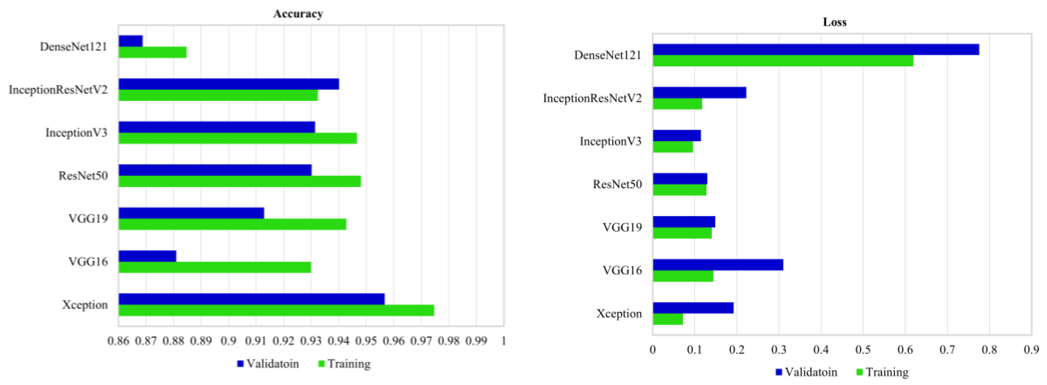
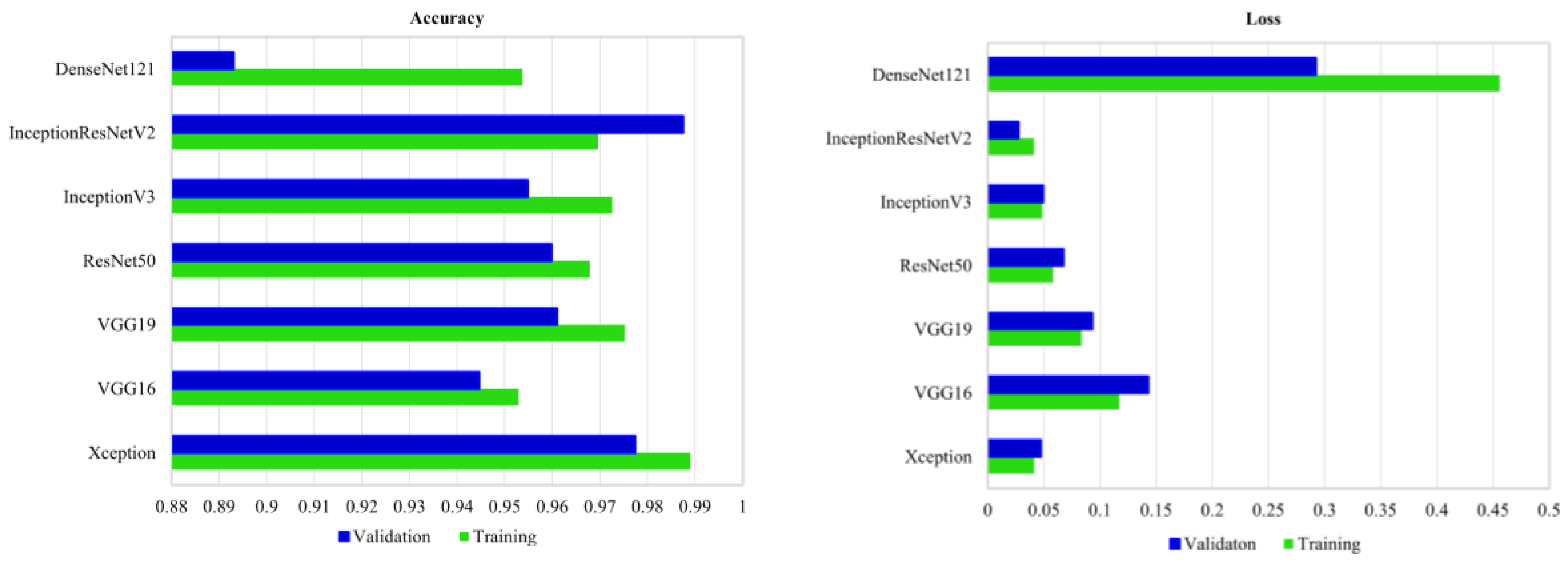
In this study, fine-tuning was employed for pre-existing, well-known convnets, which were trained based on the ImageNet dataset. Figure 9 demonstrates the validation and training accuracy and loss in the case of fine-tuning of convnets using the three selected bands of RapidEye imagery.
As shown, DenseNet121 has the lowest validation accuracy, followed by VGG16. Conversely, the Xception network has the highest validation accuracy, followed by InceptionResNetV2. The two convnets, namely InceptionV3 and ResNet50, show relatively equal validation accuracies. Figure 10 shows the validation and training accuracy and loss in the case of training convnets from scratch when three bands of RapidEye imagery were employed.
As shown, all convnets, excluding DensNet121, perform very well for wetland classification when validation accuracies are compared. In particular, three convnets, including InceptionResNetV2, Xception, and VGG19, have higher training and validation accuracies relative to the other well-known convnets. Conversely, DenseNet121 has the lowest validation accuracy, suggesting that this network is less suitable for complex land cover mapping relative to the other convnets. Figure 11 shows the validation and training accuracy and loss in the case of training convnets from scratch when five bands of RapidEye imagery were employed.
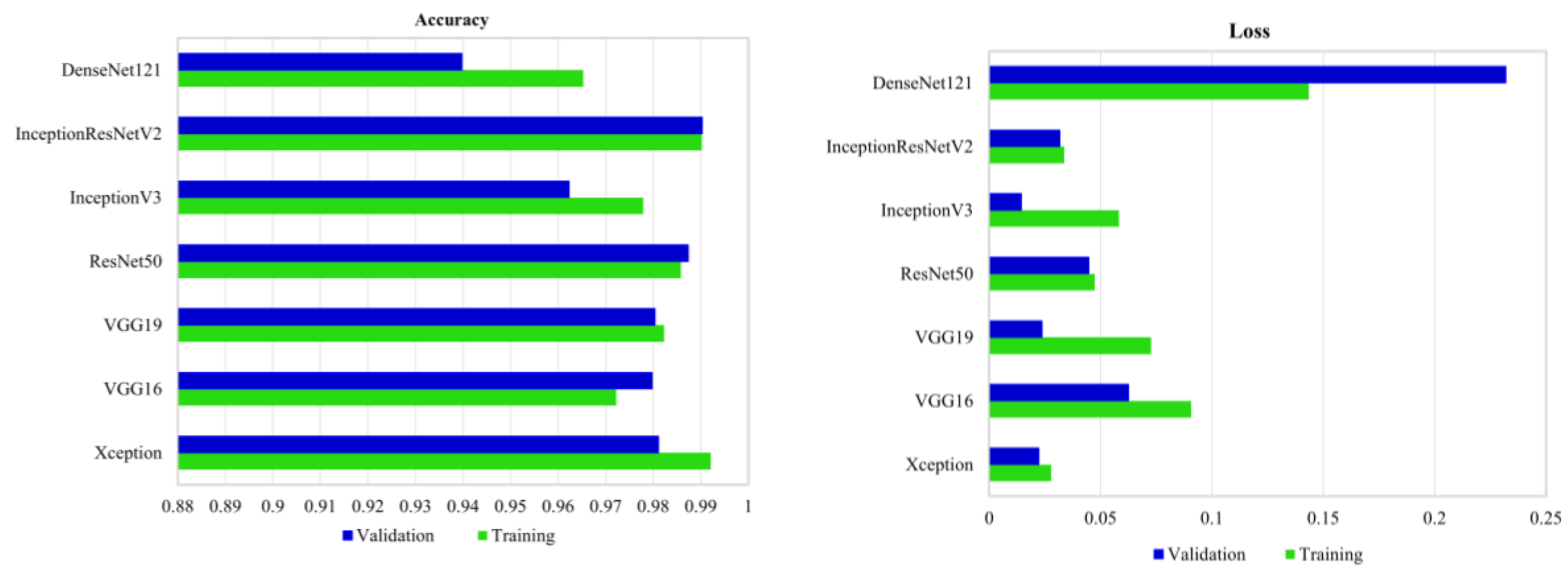
The effects of increasing the number of bands are readily apparent by comparing Figure 10 and Figure 11. Specifically, an increase in the number of bands improves classification accuracy in all cases. For example, the validation accuracy for DenseNet121 was lower than 90% when only three bands were employed. However, by increasing the number of bands, the validation accuracy reached to 94% for DenseNet121. InceptionResNetV2 again exhibited the highest validation accuracy, followed by ResNet50, Xception, and VGG19. Thus, the results indicate the significance of incorporating more spectral information for the classification of spectrally similar wetland classes (see Figure 10 and Figure 11).
One of the most interesting aspects of the results obtained in this study is that the full-training strategy had better classification results relative to fine-tuning in all cases. Previous studies reported the superiority of fine-tuning relative to full-training for classification of very high resolution aerial imagery, although full-training was found to be more accurate relative to fine-tuning for classification of multi-spectral satellite data [26,45]. In particular, Nogueira et al. (2017) evaluated the efficiency of fine-tuning and full-training strategies of some well-known deep CNNs (e.g., AlexNet and GoogLeNet) for classification of three well-known datasets, including UCMerced land-use [46], RS19 dataset [47], and Brazilian Coffee Scenes [48]. The fine-tuning strategy yielded a higher accuracy for the first two datasets, likely due to their similarity with the ImageNet dataset, which was originally used for training deep CNNs. However, the full-training strategy had similar [26] or better results [45] relative to the fine-tuning for the Brazilian Coffee Scenes. This is because the latter dataset is multi-spectral (SPOT), containing finer and more homogeneous textures, wherein the patterns visually overlap substantially and, importantly, differ from the objects commonly found within the ImageNet dataset [26]. The results obtained from the latter dataset are similar to those found in our study. In particular, there is a significant difference between the original training datasets of these convnets and our dataset. Fine-tuning is an optimal solution when the edges and local structures within the dataset of interest are similar to those for which the networks were trained. However, the texture, color, edges, and local structures of the typical objects found in the ImageNet dataset differ from the objects found in the wetland classes. Moreover, our dataset is intrinsically different from the ImageNet dataset used for pre-training. In particular, our dataset has five spectral bands, namely red, green, blue, red-edge, and near-infrared, all of which are essential for classifying spectrally similar wetland classes. However, the ImageNet dataset has only the red, green, and blue bands [45]. This could explain the differences between validation accuracies obtained in the case of full-training and fine-tuning (see Figure 9 and Figure 10). Nevertheless, the results obtained from fine-tuning are still very promising, taking into account the complexity of wetland classes and the high classification accuracy obtained in most cases. In particular, an average validation accuracy of greater than 86% was achieved in all cases (see Figure 9), suggesting the generalizability and versatility of pre-trained deep convnets for the classification of various land cover types. It is also worth noting that fine-tuning was employed on the top three layers of convnets in this study. However, the results could be different upon including more layers in the fine-tuning procedure.
Having obtained higher accuracies via full-training of five bands, the classification results obtained from this strategy were selected for further analysis. These classification results were also compared with the results obtained from two conventional machine learning tools (i.e., SVM and RF). For this purpose, a total number of eight features were used as input features for both the SVM and RF classifiers. These features were Normalized Difference Vegetation Index (NDVI), Normalized Difference Water Index (NDWI), Red-edge Normalized Difference Vegetation Index (ReNDVI), and all the original spectral bands of the RapidEye image. Table 2 represents the overall accuracy, Kappa coefficient, and F1-score using different CNNs (full-training of five bands), RF, and SVM for wetland classification in this study.
As seen in Table 2, SVM and RF have the lowest classification accuracies and F1-scores relative to all deep convnets in this study. Among deep convnets, InceptionResNetV2 has the highest classification accuracy, 96.17%, as well as the highest F1-score, 93.66%, followed by ResNet50 and Xception with overall accuracies of 94.81% and 93.57%, as well as F1-scores of 91.39% and 89.55%, respectively. Conversely, DenseNet121 and InceptionV3 have the lowest overall accuracies, 84.78% and 86.14%, as well as F1-scores, 72.61% and 75.09%, respectively. VGG19 was found to be more accurate than VGG16 by about 3% (OA), presumably due to the deeper structure of the former convnet. These results are in general agreement with [49], which reported the superiority of ResNet relative to GoogLeNet (Inception), VGG16, and VGG19 for the classification of four public remote sensing datasets (e.g., UCM, WHU-RS19). InceptionResNetV2 benefits from integrating two well-known deep convnets, Inception and ResNet, which positively contribute to the most accurate result in this study. This also suggests that the extracted features from different convnets are supplementary and improve the model’s classification efficiency. The results demonstrated that deeper networks (e.g., InceptionResNetV2) have a greater efficiency in extracting varying degrees of abstraction and representation within the hierarchical learning scheme [50]. In particular, they are more efficient in separating the input space into more detailed regions, owing to their deeper architecture, that contributes to a better separation of complex wetland classes.
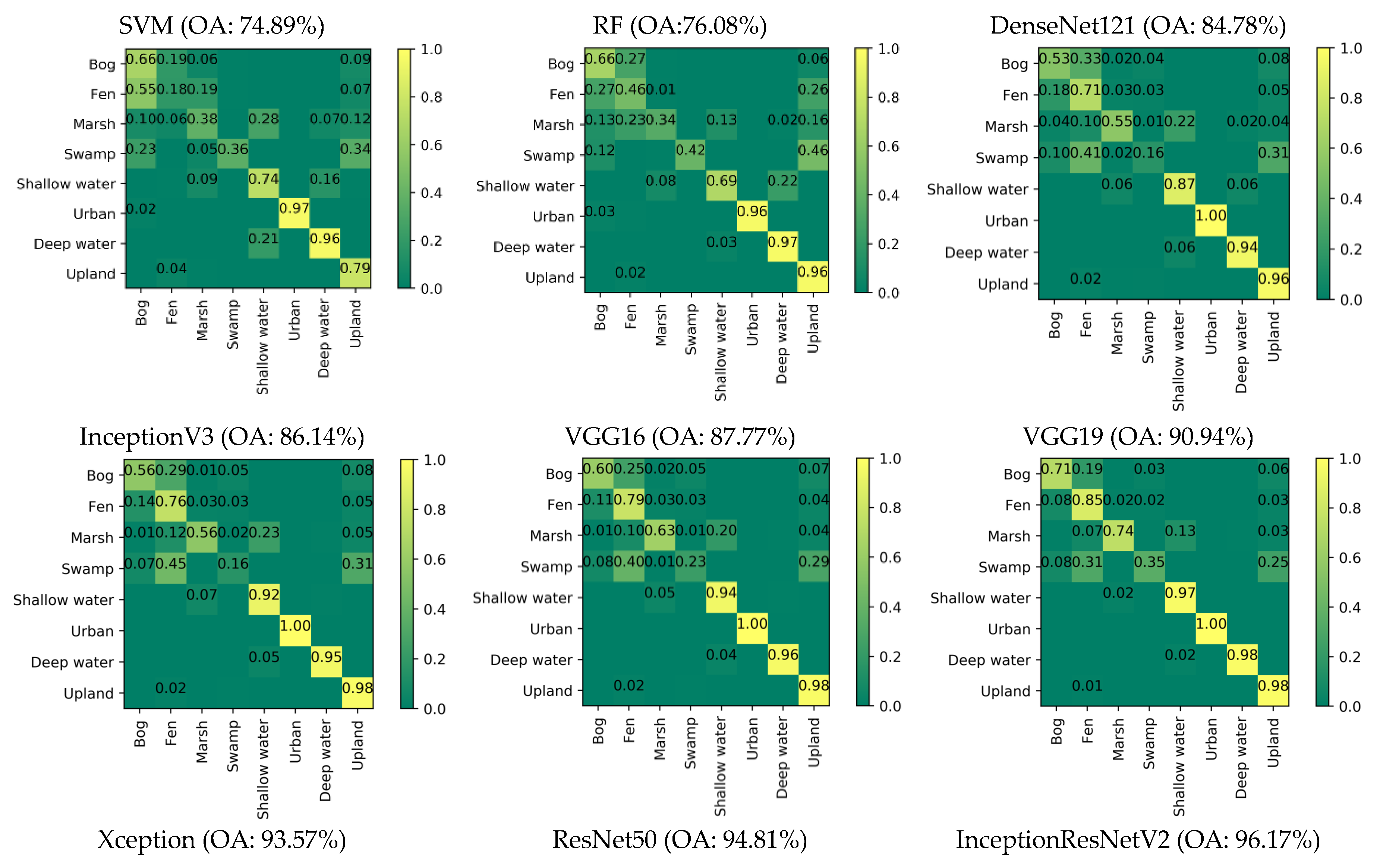
As shown in Figure 12, all deep networks were successful in classifying non-wetland classes, including urban, deep water, and upland classes, with an accuracy greater than 94% in all cases. SVM and RF also correctly classified the non-wetland classes with an accuracy exceeding 96% in most cases (excluding upland). Interestingly, all deep networks correctly classified the urban class with an accuracy of 100%, suggesting the robustness of the deep learning features for classification of complex human-made structures (e.g., buildings and roads). This observation fits well with [13]. However, the accuracy of the urban class did not exceed 97% when either RF or SVM was employed.
The confusion matrices demonstrate that, by using the last three networks, a significant improvement was achieved in the accuracy of both overall and individual classes. In particular, InceptionResNetV2 correctly classified non-wetland classes with an accuracy of 99% for deep water and 100% for both urban and upland classes. ResNet50 and Xception were also successful in distinguishing non-wetland classes with an accuracy of 100% for urban and 99% for both deep water and upland. One possible explanation for why the highest accuracies were obtained for these classes is the availability of larger amounts of training samples for non-wetland classes relative to wetland classes.
Although RF and SVM, as well as the convnets, performed very well in distinguishing non-wetland classes, the difference in accuracy between the two groups (i.e., conventional classifiers versus deep networks) was significant for wetland classes. This was particularly true for the last three convnets compared to SVM and RF. Specifically, the three networks of InceptionResNetV2, ResNet50, and Xception were successful in classifying all wetland classes with accuracies exceeding 80%, excluding the swamp wetland. This contrasts with the results obtained from SVM and RF, wherein the accuracies were lower than 74% for all wetland classes. Overall, the swamp wetland had the lowest accuracy among all classes using the deep convnets. As the effectiveness of these networks largely depends on the numbers of the training samples, the lowest accuracy of the swamp wetland could be attributable to the low availability of training samples for this class.
A large degree of confusion was observed between herbaceous wetlands, namely marsh, bog, and fen (especially between bog and fen), when DenseNet121, InceptionV3, and VGG16 were employed. The largest confusion between bog and fen is possibly due to the very similar visual features of these classes (see Figure 8). These two classes are both peatland dominated with different species of Sphagnum in bogs and Graminoid in fens. According to field biologist reports, these two classes were adjacent successional classes with a heterogeneous nature and were hardly distinguished from each other during the in-situ field data collection.
Overall, confusion was more pronounced among the first four deep networks, whereas it was significantly reduced when the last three networks were employed (see Figure 12). This suggests that the last three networks and, especially, InceptionResNetV2, are superior for distinguishing confusing wetland classes relative to the other convnets. For example, the classes of bog and fen were correctly classified with accuracies of greater than 89% when InceptionResNetV2 was used. Both Xception and ResNet50 were also found to successfully classify these two classes with accuracies of higher than 80%. Overall, the wetland classification accuracies obtained from these three networks were strongly positive for several spectrally and spatially similar wetland classes (e.g., bog, fen, and marsh) and demonstrate a large number of correctly classified pixels.
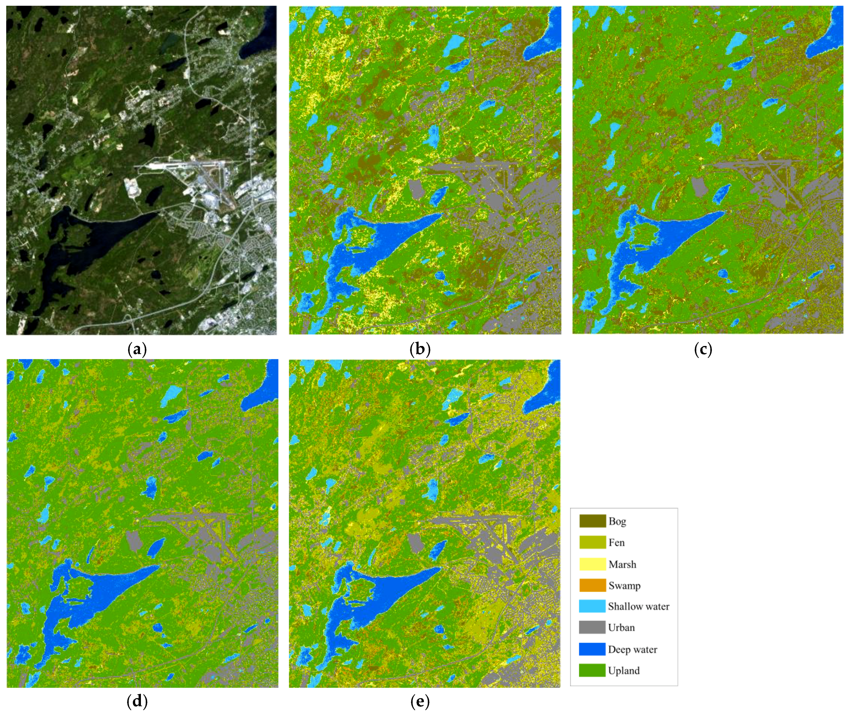
Cropped images of the classified maps obtained from SVM, RF, DenseNet121, and InceptionResNetV2 are depicted in Figure 13. As shown, the classified maps obtained from convnets better resemble the real ground features. Both classified maps, obtained from convnets (Figure 13d,e) show a detailed distribution of all land cover classes; however, the classified map obtained from InceptionResNetV2 (Figure 13e) is more accurate when it is compared with optical imagery (Figure 13a). For example, in the classified map obtained from DenseNet121, the fen class was misclassified as bog and upland classes in some cases (Figure 13d). This, too, occurred between shallow water and deep water; however, this was not the case when InceptionResNetV2 was employed. In particular, most land cover classes obtained from InceptionResNetV2 are accurate representations of ground features. This conclusion was based on the confusion matrix (see Figure 12) and further supported by a comparison between the classified map and the optical data (Figure 13a, e).
Figure 14 shows two-dimensional features extracted from the last layer of the InceptionResNetV2 (a) and DenseNet121 (b) using the two-dimensional t-SNE algorithm [51]. The features from InceptionResNetV2 demonstrate a clear semantic clustering. In particular, most classes are clearly separated from each other; however, the feature clusters of bog and fen show some degree of confusion. Conversely, the features from DenseNet121 only generate a few visible clusters (e.g., upland and urban), while other features corresponding to wetland classes overlap with each other, suggesting a large degree of confusion.

4. Conclusions

Wetlands are characterized by complex land cover with high intra-class variability and low inter-class disparity, posing several challenges to conventional machine learning tools in classification tasks. To date, the discrimination of such complex land cover classes using conventional classifiers heavily relies on a large number of hand-crafted features incorporated into the classification scheme. In this research, we used state-of-the-art deep learning tools, deep Convolutional Neural Networks, to classify such a heterogeneous environment to address the problem of extracting a large number of hand-crafted features. Two different strategies of employing pre-existing convnets were investigated: Full-training and fine-tuning. The potential of the most well-known deep convnets, currently employed for several computer vision tasks, including DenseNet121, InceptionV3, VGG16, VGG19, Xception, ResNet50, and InceptionResNetV2, was examined in a comprehensive and elaborate framework using multispectral RapidEye optical data for wetland classification.
The results of this study revealed that the incorporation of high-level features learned by a hierarchical deep framework is very efficient for the classification of complex wetland classes. Specifically, the results illustrate that the full-training of pre-existing convnets using five bands is more accurate than both full-training and fine-tuning using three bands, suggesting that the extra multispectral bands provide complementary information. In this study, InceptionResNetV2 consistently outperformed all other convnets for the classification of wetland and non-wetland classes with a state-of-the-art overall classification accuracy of about 96%, followed by ResNet50 and Xception, with accuracies of about 94% and 93%, respectively. The impressive performance of InceptionResNetV2 suggests that an integration of the Inception and ResNet modules is an effective architecture for complex land cover mapping using multispectral remote sensing images. The individual class accuracy illustrated that confusion occurred between wetland classes (herbaceous wetlands), although it was less pronounced when InceptionResNetV2, ResNet50, and Xception were employed. The swamp wetland had the lowest accuracy in all cases, potentially because the lowest number of training samples was available for this class. It is also worth noting that all deep convnets were very successful in classifying non-wetland classes in this study.
The results of this study demonstrate the potential for the full exploitation of pre-existing deep convnets for the classification of multispectral remote sensing data, which are significantly different than large datasets (e.g., ImageNet) currently employed in computer vision. Given the similarity of wetland classes across Canada, the deep trained networks in this study provide valuable baseline information and tools, and will substantially contribute to the success of wetland mapping in this country using state-of-the-art remote sensing data.
Author Contributions

All authors made substantial contributions to conception and design the study. M.M., M.R., and F.M. performed the experiments, analyzed the data, and wrote the paper. All authors reviewed and commented on the manuscript.

Funding

This project was undertaken with the financial support of the Government of Canada through the federal Department of Environment and Climate Change, the Research & Development Corporation of Newfoundland and Labrador (RDC 5404-2108-101), and the Natural Sciences and Engineering Research Council of Canada (NSERC RGPIN2015-05027).

Acknowledgments

Field data were collected by various organizations, including Ducks Unlimited Canada, Government of Newfoundland and Labrador Department of Environment and Conservation, and Nature Conservancy Canada. The authors thank these organizations for the generous financial support and providing such valuable datasets. Also, the authors would like to thank the anonymous reviewers for their helpful comments and suggestions.

Conflicts of Interest

The authors declare no conflicts of interest.

References

  1. Tiner, R.W.; Lang, M.W.; Klemas, V.V. Remote Sensing of Wetlands: Applications and Advances; CRC Press: Boca Raton, FL, USA, 2015. [Google Scholar]
  2. Mahdianpari, M.; Salehi, B.; Mohammadimanesh, F.; Motagh, M. Random forest wetland classification using ALOS-2 L-band, RADARSAT-2 C-band, and TerraSAR-X imagery. ISPRS J. Photogramm. Remote Sens. 2017, 130. [Google Scholar] [CrossRef]
  3. Evans, T.L.; Costa, M. Landcover Classification of the Lower Nhecolândia Subregion of the Brazilian Pantanal Wetlands Using Alos/Palsar, Radarsat-2 and Envisat/Asar Imagery. Remote Sens. Environ. 2013, 128, 118–137. [Google Scholar] [CrossRef]
  4. Mahdianpari, M.; Salehi, B.; Mohammadimanesh, F. The Effect of Polsar Image De-Speckling on Wetland Classification: Introducing a New Adaptive Method. Can. J. Remote Sens. 2017, 43, 485–503. [Google Scholar] [CrossRef]
  5. Mahdianpari, M.; Salehi, B.; Mohammadimanesh, F.; Brisco, B.; Mahdavi, S.; Amani, M.; Granger, J.E. Fisher Linear Discriminant Analysis of Coherency Matrix for Wetland Classification Using Polsar Imagery. Remote Sens. Environ. 2018, 206. [Google Scholar] [CrossRef]
  6. Mohammadimanesh, F.; Salehi, B.; Mahdianpari, M.; Brisco, B.; Motagh, M. Multi-Temporal, Multi-Frequency, and Multi-Polarization Coherence and Sar Backscatter Analysis of Wetlands. ISPRS J. Photogramm. Remote Sens. 2018, 142, 78–93. [Google Scholar] [CrossRef]
  7. Adam, E.; Mutanga, O.; Rugege, D. Multispectral and Hyperspectral Remote Sensing for Identification and Mapping of Wetland Vegetation: A Review. Wetl. Ecol. Manag. 2010, 18, 281–296. [Google Scholar] [CrossRef]
  8. Friedl, M.A.; Brodley, C.E. Decision Tree Classification of Land Cover from Remotely Sensed Data. Remote Sens. Environ. 1997, 61, 399–409. [Google Scholar] [CrossRef]
  9. Mohammadimanesh, F.; Salehi, B.; Mahdianpari, M.; Motagh, M.; Brisco, B. An efficient feature optimization for wetland mapping by synergistic use of SAR intensity, interferometry, and polarimetry data. Int. J. Appl. Earth Obs. Geoinf. 2018, in press. [Google Scholar] [CrossRef]
  10. Rezaee, M.; Mahdianpari, M.; Zhang, Y.; Salehi, B. Deep Convolutional Neural Network for Complex Wetland Classification Using Optical Remote Sensing Imagery. IEEE J. Sel. Top. Appl. Earth Obs. Remote Sens. 2018. [Google Scholar] [CrossRef]
  11. Mahdianpari, M.; Salehi, B.; Mohammadimanesh, F.; Brisco, B. An Assessment of Simulated Compact Polarimetric Sar Data for Wetland Classification Using Random Forest Algorithm. Can. J. Remote Sens. 2017, 43. [Google Scholar] [CrossRef]
  12. Blaschke, T. Object Based Image Analysis for Remote Sensing. ISPRS J. Photogramm. Remote Sens. 2010, 65, 2–16. [Google Scholar] [CrossRef]
  13. Zhao, W.; Du, S. Learning Multiscale and Deep Representations for Classifying Remotely Sensed Imagery. ISPRS J. Photogramm. Remote Sens. 2016, 113, 155–165. [Google Scholar] [CrossRef]
  14. Jackson, Q.; Landgrebe, D.A. Adaptive Bayesian Contextual Classification Based on Markov Random Fields. IEEE Trans. Geosci. Remote Sens. 2002, 40, 2454–2463. [Google Scholar] [CrossRef]
  15. Zhong, P.; Wang, R. Learning Conditional Random Fields for Classification of Hyperspectral Images. IEEE Trans. Image Process. 2010, 19, 1890–1907. [Google Scholar] [CrossRef] [PubMed]
  16. Camps-Valls, G.; Gomez-Chova, L.; Muñoz-Marí, J.; Vila-Francés, J.; Calpe-Maravilla, J. Composite Kernels for Hyperspectral Image Classification. IEEE Geosci. Remote Sens. Lett. 2006, 3, 93–97. [Google Scholar] [CrossRef]
  17. Chollet, F. Deep Learning with Python; Manning Publications Co.: Greenwich, CT, USA, 2017. [Google Scholar]
  18. LeCun, Y.; Bengio, Y.; Hinton, G. Deep Learning. Nature 2015, 521, 436. [Google Scholar] [CrossRef] [PubMed]
  19. Ball, J.E.; Anderson, D.T.; Chan, C.S. Comprehensive Survey of Deep Learning in Remote Sensing: Theories, Tools, and Challenges for the Community. J. Appl. Remote Sens. 2017, 11, 042609. [Google Scholar] [CrossRef]
  20. Hinton, G.E.; Osindero, S.; Teh, Y.-W. A Fast Learning Algorithm for Deep Belief Nets. Neural Comput. 2006, 18, 1527–1554. [Google Scholar] [CrossRef] [PubMed] [Green Version]
  21. Vincent, P.; Larochelle, H.; Lajoie, I.; Bengio, Y.; Manzagol, P.-A. Stacked Denoising Autoencoders: Learning Useful Representations in a Deep Network with a Local Denoising Criterion. J. Mach. Learn. Res. 2010, 11, 3371–3408. [Google Scholar]
  22. Krizhevsky, A.; Sutskever, I.; Hinton, G.E. Imagenet Classification with Deep Convolutional Neural Networks. In Proceedings of the 25th International Conference on Neural Information Processing Systems, Lake Tahoe, NV, USA, 3–6 December 2012; pp. 1097–1105. [Google Scholar]
  23. Szegedy, C.; Liu, W.; Jia, Y.; Sermanet, P.; Reed, S.; Anguelov, D.; Erhan, D.; Vanhoucke, V.; Rabinovich, A. Going Deeper with Convolutions. In Proceedings of the IEEE Conference on Computer Vision and Pattern Recognition (CVPR), Boston, MA, USA, 7–12 June 2015. [Google Scholar]
  24. Marmanis, D.; Schindler, K.; Wegner, J.D.; Galliani, S.; Datcu, M.; Stilla, U. Classification with an Edge: Improving Semantic Image Segmentation with Boundary Detection. ISPRS J. Photogramm. Remote Sens. 2018, 135, 158–172. [Google Scholar] [CrossRef]
  25. Chen, X.; Xiang, S.; Liu, C.-L.; Pan, C.-H. Vehicle Detection in Satellite Images by Hybrid Deep Convolutional Neural Networks. IEEE Geosci. Remote Sens. Lett. 2014, 11, 1797–1801. [Google Scholar] [CrossRef]
  26. Nogueira, K.; Penatti, O.A.B.; dos Santos, J.A. Towards Better Exploiting Convolutional Neural Networks for Remote Sensing Scene Classification. Pattern Recognit. 2017, 61, 539–556. [Google Scholar] [CrossRef]
  27. LeCun, Y.; Bottou, L.; Bengio, Y.; Haffner, P. Gradient-Based Learning Applied to Document Recognition. Proc. IEEE 1998, 86, 2278–2324. [Google Scholar] [CrossRef]
  28. Deng, J.; Dong, W.; Socher, R.; Li, L.-J.; Li, K.; Li, F.-F. Imagenet: A Large-Scale Hierarchical Image Database. In Proceedings of the IEEE Conference on Computer Vision and Pattern Recognition, Miami, FL, USA, 20–25 June 2009. [Google Scholar]
  29. Simonyan, K.; Zisserman, A. Very Deep Convolutional Networks for Large-Scale Image Recognition. arXiv 2014, arXiv:1409.1556. [Google Scholar]
  30. He, K.; Zhang, X.; Ren, S.; Sun, J. Deep Residual Learning for Image Recognition. In Proceedings of the IEEE Conference on Computer Vision and Pattern Recognition (CVPR), Las Vegas, NV, USA, 27–30 June 2016; pp. 770–778. [Google Scholar]
  31. Chollet, F. Xception: Deep Learning with Depthwise Separable Convolutions. arXiv 2016, arXiv:1610.02357. [Google Scholar]
  32. Hu, F.; Xia, G.-S.; Hu, J.; Zhang, L. Transferring Deep Convolutional Neural Networks for the Scene Classification of High-Resolution Remote Sensing Imagery. Remote Sens. 2015, 7, 14680–14707. [Google Scholar] [CrossRef] [Green Version]
  33. Hinton, G.E.; Salakhutdinov, R.R. Reducing the Dimensionality of Data with Neural Networks. Science 2006, 313, 504–507. [Google Scholar] [CrossRef] [PubMed]
  34. Zhang, L.; Zhang, L.; Du, B. Deep Learning for Remote Sensing Data: A Technical Tutorial on the State of the Art. IEEE Geosci. Remote Sens. Mag. 2016, 4, 22–40. [Google Scholar] [CrossRef]
  35. Kang, M.; Ji, K.; Leng, X.; Xing, X.; Zou, H. Synthetic Aperture Radar Target Recognition with Feature Fusion Based on a Stacked Autoencoder. Sensors 2017, 17, 192. [Google Scholar] [CrossRef] [PubMed]
  36. Nair, V.; Hinton, G.E. Rectified Linear Units Improve Restricted Boltzmann Machines. In Proceedings of the 27th International Conference on International Conference on Machine Learning, Haifa, Israel, 21–24 June 2010; pp. 807–814. [Google Scholar]
  37. Sifre, L.; Mallat, S. Rotation, Scaling and Deformation Invariant Scattering for Texture Discrimination. In Proceedings of the IEEE Conference on Computer Vision and Pattern Recognition, Portland, OR, USA, 23–28 June 2013; pp. 1233–1240. [Google Scholar]
  38. Szegedy, C.; Ioffe, S.; Vanhoucke, V.; Alemi, A.A. Inception-V4, Inception-Resnet and the Impact of Residual Connections on Learning. arXiv 2017, arXiv:1602.07261. [Google Scholar]
  39. Huang, G.; Liu, Z.; Weinberger, K.Q.; van der Maaten, L. Densely Connected Convolutional Networks. arXiv 2017, arXiv:1608.06993. [Google Scholar] [Green Version]
  40. Makantasis, K.; Karantzalos, K.; Doulamis, A.; Doulamis, N. Deep Supervised Learning for Hyperspectral Data Classification through Convolutional Neural Networks. In Proceedings of the IEEE International Geoscience and Remote Sensing Symposium (IGARSS), Milan, Italy, 26–31 July 2015; pp. 4959–4962. [Google Scholar]
  41. Zhang, C.; Pan, X.; Li, H.; Gardiner, A.; Sargent, I.; Hare, J.; Atkinson, P.M. A Hybrid MLP-CNN Classifier for Very Fine Resolution Remotely Sensed Image Classification. ISPRS J. Photogramm. Remote Sens. 2017, 140, 133–144. [Google Scholar] [CrossRef]
  42. Mnih, V. Machine Learning for Aerial Image Labeling; University of Toronto: Toronto, ON, Canada, 2013. [Google Scholar]
  43. Abadi, M.; Agarwal, A.; Barham, P.; Brevdo, E.; Chen, Z.; Citro, C.; Corrado, G.S.; Davis, A.; Dean, J.; Devin, M. Tensorflow: Large-Scale Machine Learning on Heterogeneous Distributed Systems. arXiv 2016, arXiv:1603.04467. [Google Scholar]
  44. Liu, Y.; Fan, B.; Wang, L.; Bai, J.; Xiang, S.; Pan, C. Semantic Labeling in Very High Resolution Images Via a Self-Cascaded Convolutional Neural Network. ISPRS J. Photogramm. Remote Sens. 2017. [Google Scholar] [CrossRef]
  45. Castelluccio, M.; Poggi, G.; Sansone, C.; Verdoliva, L. Land Use Classification in Remote Sensing Images by Convolutional Neural Networks. arXiv 2015, arXiv:1508.00092. [Google Scholar]
  46. Yang, Y.; Newsam, S. Bag-of-Visual-Words and Spatial Extensions for Land-Use Classification. In Proceedings of the 18th SIGSPATIAL International Conference on Advances in Geographic Information Systems, San Jose, CA, USA, 2–5 November 2010. [Google Scholar]
  47. Xia, G.-S.; Yang, W.; Delon, J.; Gousseau, Y.; Sun, H.; Maître, H. Structural High-Resolution Satellite Image Indexing. In Proceedings of the ISPRS TC VII Symposium-100 Years ISPRS, Vienna, Austria, 5–7 July 2010. [Google Scholar]
  48. Penatti, O.A.; Nogueira, K.; dos Santos, J.A. Do Deep Features Generalize from Everyday Objects to Remote Sensing and Aerial Scenes Domains? In Proceedings of the 2015 IEEE Conference on Computer Vision and Pattern Recognition Workshops (CVPRW), Boston, MA, USA, 7–12 June 2015. [Google Scholar]
  49. Han, W.; Feng, R.; Wang, L.; Cheng, Y. A Semi-Supervised Generative Framework with Deep Learning Features for High-Resolution Remote Sensing Image Scene Classification. ISPRS J. Photogramm. Remote Sens. 2017. [Google Scholar] [CrossRef]
  50. Chen, Y.; Lin, Z.; Zhao, X.; Wang, G.; Gu, Y. Deep Learning-Based Classification of Hyperspectral Data. IEEE J. Sel. Top. Appl. Earth Obs. Remote Sens. 2014, 7, 2094–2107. [Google Scholar] [CrossRef]
  51. Maaten, L.v.d.; Hinton, G. Visualizing Data Using t-SNE. J. Mach. Learn. Res. 2008, 9, 2579–2605. [Google Scholar]
Figure 1. Schematic diagram of (a) VGG16 and (b) VGG19 models.
Remotesensing 10 01119 g001
Figure 2. Schematic diagram of InceptionV3 model (compressed view).
Remotesensing 10 01119 g002
Figure 3. Schematic diagram of ResNet model (compressed view).
Remotesensing 10 01119 g003
Figure 4. Schematic diagram of Xception model (compressed view).
Remotesensing 10 01119 g004
Figure 5. Schematic diagram of InceptionResNetV2 model (compressed view).
Remotesensing 10 01119 g005
Figure 6. Schematic diagram of DenseNet model (compressed view).
Remotesensing 10 01119 g006
Figure 7. A true color composite of RapidEye optical imagery (bands 3, 2, and 1) acquired on 18 June, 2015, illustrating the geographic location of the study area. The red rectangle, the so-called test-zone, was selected to display the classified maps obtained from different approaches. Note that the training samples within the rectangle were excluded during the training stage for deep Convolutional Neural Networks (CNNs).
Remotesensing 10 01119 g007
Figure 8. Ground reference photos showing land cover classes in the study area: (a) Bog; (b) fen; (c) marsh; (d) swamp; (e) shallow water; (f) urban; (g) deep water; and (h) upland.
Remotesensing 10 01119 g008
Figure 9. Comparing well-known convnets in terms of training and validation accuracy and loss when fine-tuning of three bands (i.e., Green, Red, and near-infrared (NIR)) was employed for complex wetland mapping.
Remotesensing 10 01119 g009
Figure 10. Comparing well-known convnets in terms of training and validation accuracy and loss when networks were trained from scratch using three bands (i.e., Green, Red, and NIR) for complex wetland mapping.
Remotesensing 10 01119 g010
Figure 11. Comparing well-known convnets in terms of training and validation accuracy and loss when networks were trained from scratch using five bands for complex wetland mapping.
Remotesensing 10 01119 g011
Figure 12. Normalized confusion matrix of the wetland classification for different networks in this study (full-training of five optical bands), Random Forest (RF), and Support Vector Machine (SVM).
Remotesensing 10 01119 g012aRemotesensing 10 01119 g012b
Figure 13. (a) True color composite of RapidEye optical imagery (bands 3, 2, and 1). A crop of the classified maps obtained from (b) SVM, (c) RF, (d) DenseNet121, and (e) InceptionResNetV2.
Remotesensing 10 01119 g013
Figure 14. A 2-D feature visualization of global image representation of the wetland classes using the t-SNE algorithm for the last layer of (a) InceptionResNetV2 and (b) DenseNet121. Each color illustrates a different class in the dataset.
Remotesensing 10 01119 g014
Table 1. The characteristics of deep convnets examined in this study.
ConvNet ModelsParameters (millions)DepthProcessing Time 1 (s)
VGG161382318
VGG191442621
InceptionV32415910
ResNet502616812
Xception2312616
InceptionResNetV25657219
DenseNet121812114
1 Note: The processing time was calculated for training of 800 images (100 images for each class).
Table 2. Overall accuracies (%), Kappa coefficients, and F1-score (%) for wetland classification using different deep convnets (full-training of five bands), Random Forest (RF), and Support Vector Machine (SVM).
MethodsOverall AccuracyKappa CoefficientF1
SVM74.890.6853.58
RF76.080.7058.87
DenseNet12184.780.8072.61
InceptionV386.140.8275.09
VGG1687.770.8478.13
VGG1990.940.8884.20
Xception93.570.9289.55
ResNet5094.810.9391.39
InceptionResNetV296.170.9593.66