Atmospheric Correction of OLCI Imagery over Extremely Turbid Waters Based on the Red, NIR and 1016 nm Bands and a New Baseline Residual Technique

Abstract

A common approach to the pixel-by-pixel atmospheric correction of satellite water colour imagery is to calculate aerosol and water reflectance at two spectral bands, typically in the near infra-red (NIR, 700–1000 nm) or the short-wave-infra-red (SWIR, 1000–3000 nm), and then extrapolate aerosol reflectance to shorter wavelengths. For clear waters, this can be achieved simply for NIR bands, where the water reflectance can be assumed negligible i.e., the “black water” assumption. For moderately turbid waters, either the NIR water reflectance, which is non-negligible, must be modelled or longer wavelength SWIR bands, with negligible water reflectance, must be used. For extremely turbid waters, modelling of non-zero NIR water reflectance becomes uncertain because the spectral slopes of water and aerosol reflectance in the NIR become similar, making it difficult to distinguish between them. In such waters the use of SWIR bands is definitely preferred and the use of the MODIS bands at 1240 nm and 2130 nm is clearly established although, on many sensors such as the Ocean and Land Colour Instrument (OLCI), such SWIR bands are not included. Instead, a new, cheaper SWIR band at 1016 nm is available on OLCI with potential for much better atmospheric correction over extremely turbid waters. That potential is tested here. In this work, we demonstrate that for spectrally-close band triplets (such as OLCI bands at 779–865–1016 nm), the Rayleigh-corrected reflectance of the triplet’s “middle” band after baseline subtraction (or baseline residual, BLR) is essentially independent of the atmospheric conditions. We use the three BLRs defined by three consecutive band triplets of the group of bands 620–709–779–865–1016 nm to calculate water reflectance and hence aerosol reflectance at these wavelengths. Comparison with standard atmospheric correction algorithms shows similar performance in moderately turbid and clear waters and a considerable improvement in extremely turbid waters.

1. Introduction

The National Aeronautics and Space Administration (NASA) SeaDAS standard atmospheric correction algorithm applied to MODIS (Moderate Resolution Imaging Spectroradiometer) imagery uses two bands in the near infra-red (NIR) at 765 and 865 nm, assuming zero water-leaving radiance contribution (“black water” hypothesis) at these bands (Gordon and Wang 1994 [1]) or, for turbid waters, modelling the NIR water reflectance with an iterative process (Stumpf et al., 2003 [2]). The aerosol reflectance at the NIR bands is then used to estimate aerosol properties and hence extrapolate aerosol reflectance (and diffuse transmittance) to the visible (VIS) bands. For extremely turbid waters, (e.g., ${\rho }_w\left(865\mathrm{nm}\right)>0.02$ with suspended particulate matter (SPM) concentration above $100{\mathrm{g}/\mathrm{m}}^3$), this procedure may fail because of one or more problems:

P1. 

The NIR water reflectance spectrum becomes flatter (Doxaran et al., 2002 [3]) and hence more similar to aerosol reflectance spectra (Ruddick and Vanhellemont 2015 [4]);

P2. 

At high reflectance the simple analytic models of NIR water reflectance as polynomial expansions of the Gordon parameter (the ratio of $\frac{b_b}{a+b_b}$) are no longer accurate (Ruddick et al., 2006 [5]) and better modelling is needed (Lee et al., 2016 [6], Luo et al., 2018 [7]);

P3. 

Top of atmosphere (TOA) reflectance may even exceed the photodetector saturation values of certain ocean colour sensors rendering these wavelengths unusable (Dogliotti et al., 2011 [8]).

In these cases, improvements to the standard “NIR-extrapolation” procedure are needed. One approach is to apply the black water assumption at bands in the short-wave-infra-red (SWIR) (e.g., 1240, 1640 and 2130 nm in MODIS), where water absorption is much higher giving negligible water-leaving radiance even in highly turbid waters (Wang and Shi 2005 [9]). Although the European Space Agency’s (ESA) Ocean and Land Colour Instrument (OLCI) on Sentinel-3 lacks far-SWIR bands (e.g., 1240 nm, 2130 nm in MODIS), it incorporates a new SWIR band at 1016 nm (nominally 1020 nm, although here the value of 1016 nm is preferred, which corresponds to the mean wavelength of the spectral response function of the band). While the black water assumption does not hold at 1016 nm for extremely turbid water (Knaeps et al., 2012 [10]), the pure water absorption is much higher at this band than at the NIR, meaning that the flattening of the NIR water reflectance spectrum in extremely turbid waters (P1) does not extend to 1016 nm—with inclusion of this band, water-reflectance spectra have clearly different shape from aerosol reflectance spectra and decomposition of the TOA (or Rayleigh-corrected) reflectance into water and aerosol reflectance components can be achieved. NIR/SWIR extrapolative algorithms are the most conventional but clearly not the only possible approach to atmospheric correction. Considerable success has also been achieved by full spectrum coupled water-atmosphere optical models which use an optimization or iterative approach to obtain a best-fitting combination of water and atmosphere unknowns, such as in, e.g., Doerffer and Schiller 2007 [11], Chomko and Gordon 2001 [12]. Such approaches have even achieved extraordinary success in removing strong but spectrally simple sunglint (e.g., POLYMER, Steinmetz et al., 2011 [13]) and tend to always provide a water reflectance spectrum that looks like water, avoiding for example negative reflectances, and proving very robust even for data with calibration bias. The operational potential of such approaches is fully recognized, but the extrapolative approach is preferred here because each step of the process has a clear physical basis, facilitating troubleshooting and improvement. For example, a poor water reflectance model or inaccurate calibration or inappropriate aerosol model will be clearly made evident with an extrapolative approach but may be less obvious with a full spectrum coupled water–atmosphere approach. In this work, we design a pixel-by-pixel aerosol correction algorithm for turbid waters by identifying, for the OLCI Red-NIR-SWIR (RNS) bands, “atmospheric invariant” quantities which are sensitive to water reflectance but insensitive to aerosols, e.g., Philpot 1991 [14]. This approach is based on the fact that in the RNS region, aerosol reflectance is spectrally smoother than water reflectance (Ruddick and Vanhellemont 2015 [4]). To calculate directly the water reflectance, assuming only that aerosol reflectance is spectrally smooth, a “baseline residual” (BLR) algorithm is proposed here for Rayleigh-corrected reflectances at 3 RNS bands. A baseline is formed between the shortest and longest wavelength of the triplet and is subtracted from the middle wavelength to give the BLR. This approach is similar to that adopted, for example, in the fluorescence line height product (Letelier and Abott 1996 [15]) and gives a quantity, the BLR, that is invariant under spectrally-linear (or sufficiently smooth) signal addition. By calculating three different atmospherically “quasi-invariant” BLRs, defined by the Rayleigh-corrected (RC) reflectances at triplets (620–709–779 nm), (709–779–865 nm) and (779–865–1016 nm), and by applying over them an “equivalent transmittance” correction factor, it is then possible to calculate water reflectance in the RNS on a pixel-by-pixel basis even in the case of extremely turbid waters. Once the RNS water reflectance is calculated, the atmospheric correction can then revert to standard NIR/SWIR extrapolative algorithms by removing water reflectance from the Rayleigh-corrected reflectance to give aerosol reflectance in the RNS and then estimating an aerosol type and concentration in the NIR/SWIR and using tabulated models to extrapolate aerosol reflectance to all wavelengths as in Gordon and Wang 1994 [1]. Alternatively, if a full spectrum atmospheric correction is not required, it is possible to use the RNS water reflectance directly to estimate products such as turbidity (Dogliotti et al., 2015 [16], Dogliotti et al., 2016 [17]) or SPM (Nechad et al., 2010 [18], Shen et al., 2010 [19], Moreira et al., 2013 [20]), or chlorophyll-a concentration in turbid waters (Gilerson et al., 2010 [21], Gitelson 1992 [22], Gons et al., 2005 [23]).

2. Materials and Methods

The following subsections describe the different datasets used to calibrate and validate the algorithm.

2.1. In Situ Radiometric Measurements

In the present study, in situ above-surface radiometric measurements were used: (i) as input to radiative transfer simulations to compute a transmittance factor to be applied to BLRs (see Section 2 and Section 2.6) to compare between in situ and OLCI-derived BLRs (see Section 3.1). A total of 105 water reflectance measurements were selected from several field campaigns (2012–2015) performed in the Río de la Plata (RdP) (Argentina), a funnel-shaped estuary located at Eastern-Central South America (Figure 1), with mean suspended particulate matter concentrations (SPM) in the range 100–200 g/m${}^3$, reaching up to $400{\mathrm{g}/\mathrm{m}}^3$ (Framiñan and Brown 1996 [24]). The Analytic Spectral Devices (ASD FieldSpec FR) spectroradiometer works in the spectral range of 350–2500 nm (step 1 nm) and was used to measure upwelling and downwelling radiances, just above surface ($L_u^{0+}$ and $L_d^{0+}$, resp.) at relative azimuth to sun of either 135° or 90° and reciprocal zenithal angles of $\theta =\pm 40$° (angles in accordance with Mueller et al., 2003 [25]), and downwelling irradiance ($E_d^{0+}$) inferred from measuring nadir radiance at a calibrated quasi-lambertian plaque and multiplying it by $\pi$. These are combined to compute the above-surface water reflectance, ${\rho }_w^{0+}$:

$${\rho }_w^{0+}(\lambda ,W)=\pi \frac{L_u^{0+}\left(\lambda \right)-{\rho }_M\left(W\right)L_d^{0+}\left(\lambda \right)}{E_d^{0+}\left(\lambda \right)}$$

(1)

where ${\rho }_M\left(W\right)$ is the surface radiance reflectance factor taken from Mobley 1999 [26], which depends on the wind speed, W. The measurement protocol is detailed in Knaeps et al., 2012 [10], and follows the generic “Abovewater method 2” of the NASA 2003 Ocean Optics Protocols (Mueller et al., 2003 [25]). Hereafter, the superscript “$0+$” will be dropped from ${\rho }_w^{0+}$ for brevity. The following statistical quality control tests were applied to select only good quality spectra:

• $std\left({\rho }_w\left(750\right)\right)<0.05$
• $max\left\{CV\left({\rho }_w(400:900)\right)\right\}<20\%$
• $CV\left({\rho }_w\left(1016\right)\right)<20\%$

where CV stands for coefficient of variation (CV = std/mean, std = standard deviation calculated over 7 replicates), ${\rho }_w\left(750\right)$ is the water reflectance at 750 nm derived from in situ measurements and ${\rho }_w$ (400:900) is the in situ water reflectance in the range 400–900 nm.

2.2. Radiative Transfer Simulations

Simulations were performed to compare the behavior of BLRs computed from above-water reflectances, $BLR\left({\rho }_w\right)$, and BLRs computed from RC reflectances, $BLR\left({\rho }_{RC}\right)$, and also to establish an equivalent transmittance factor to be applied to BLRs computed from RC reflectances from OLCI scenes (see Section 2.6). In situ radiometric measurements were used as an input to the CNES-SOS v5.0 (Centre National d’Études Spatiales-Successive Orders of Scattering) radiative transfer (RT) code (Lenoble et al., 2007 [27]) to test how water reflectance baseline residuals (defined in Equations (5)–(6)) relate to Rayleigh-corrected baseline residuals taking account of atmospheric transmittance. CNES-SOS was developed to solve the vector RT equation for marine and terrestrial environments using a plane-parallel assumption. In our simulations, the surface reflectance is composed of: (i) a component that accounts for air-water interface effects, modelled as a function of surface wind speed (Cox and Munk 1954 [28]), and (ii) a component, which is assumed to be Lambertian, that accounts for radiation that interacts with the in-water constituents (also called above-water reflectance, ${\rho }_w$, Equation (1), or water-leaving radiance reflectance).

Combining all the in situ spectra with a set of multiple simulated atmospheric conditions, a total of 70875 Rayleigh-corrected (RC) reflectance spectra (

Table 1. Atmospheric, surface, geometric and spectral parameters used as input to the set of CNES-SOS simulations.

CNES-SOS Parameter	Input Values
$\lambda$ (Wavelength)	615–1040 nm (step 5 nm)
${\theta }_s$ (Solar zenith angle)	0°–60° (step 30°)
${\theta }_v$ (Viewing zenith angle)	0°–60° (step 30°)
$\Delta \varphi$ (Relative azimuth angle)	0°–180° (step 45°)
${\rho }_w$ (Water reflectance)	ASD in situ (RdP)
W (Wind speed)	3 m/s
$n_w$ (Relative air-water refractive index)	1.334
${\tau }_{ray}$ (Rayleigh optical thickness)	Bodhaine et al., 1999 [30]
${\delta }_{ray}$ (Molecular depolarization factor)	Bodhaine et al., 1999 [30]
$H_{ray}$ (Molecular e-folding height)	8 km
${\tau }_{aer}$ (Aerosol optical thickness at 500 nm)	0:0.1:0.4
$d{V}_{aer}$/$dlnr$ (Aerosol granulometry)	WMO-C, -M, -U [29]
$H_{aer}$ (Aerosol e-folding height)	2 km
$n_{max}$ (Maximum scattering order)	20
$I_{pol}$ (Polarization flag)	1 (consider polarization)

) were computed with CNES-SOS RT code, corresponding to: 3 solar and viewing zenith angles at 0°, 30° and 60° (interpolated from the Gaussian quadrature angles [27]), 5 sun-relative azimuth angles in the range 0–180° (step 45°) (where 0° represents viewing into sunglint), 3 aerosol granulometries and refractive indices of type “Continental” (WMO-C), “Maritime” (WMO-M) and “Urban” (WMO-U) (from the World Meteorological Organization aerosol optical models [29]), 5 aerosol optical depths at 500 nm in the range 0–0.4 (step 0.1) and 105 in situ water reflectances (Section 2.1). The relative refractive index of the water-air interface was fixed at $1.334$ throughout the spectrum and the wind speed fixed at 3 m/s. Rayleigh scattering from air molecules was set according to the values of Rayleigh optical thickness and depolarization factor reported by Bodhaine et al., 1999 [30], see also Mobley et al., 2016 [31]. The molecular and aerosol vertical profiles were set to follow exponential decay functions of e-folding scales of 8 km and 2 km, respectively. The code was set to not exceed 20 orders of scattering and to include the effects of polarization.

To obtain the Rayleigh-corrected reflectances of the set, the code was run twice to compute the Top-of-Atmosphere reflectance (${\rho }_{TOA}^{SOS}$): (i) using the input values specified by Table 1, and (ii) assuming a black marine environment (${\rho }_w=0$), and without aerosol content (${\rho }_a=0$). The second set was subtracted from the first to compute the RC signal, as it would be calculated in the atmospheric correction step of a satellite data processor:

$${\rho }_{RC}^{SOS}={\rho }_{TOA}^{SOS}(Air+Interface+Aerosols+Water)-{\rho }_{TOA}^{SOS}(Air+Interface)$$

(2)

2.3. Ocean and Land Colour Instrument (OLCI) Imagery

OLCI L1B and L2 imagery were downloaded from the Copernicus Online Data Access (CODA) system on 1 February 2018 [32]. The L1B and L2 imagery used in this work correspond to the processing baseline v2.23 [33]. The detailed list of scenes from Río de la Plata (RdP), Bahía Blanca (BBl, Argentina) and Belgian Coast (BE) used to calibrate and test performance of the algorithm is shown in

Table 2. List of Ocean and Land Colour Instrument (OLCI) scenes from Río de la Plata (L1B, processing baseline v2.23) used to calibrate and validate the algorithm, described by date of acquisition.

Region	Aquisition Date-Time	Calibration/Validation Window (s)	Fix Window Atmospheric Correction (Fix-AC) Window	Cal/Val
	yyyy-mm-ddThh:mm:ssZ	lines; pixels	lines; pixels	Cal
RdP	2016-08-17T12:55:02Z	1347–1636; 1258–1528	1750–1764; 1143–1157	Cal
RdP	2016-11-10T12:51:59Z	1057–1446; 521–685	1598–1612; 567–581	Cal
RdP	2016-11-29T12:58:49Z	1643–1796; 1218–1332	2117–2131; 1267–1281	Cal
RdP	2017-01-14T13:06:26Z	2254–2589; 838–1052	2655–2669; 1155–1169	Cal
RdP	2017-03-13T13:02:29Z	1890–2013; 1177–1258 2044–2124; 1130–1256	2140–2154; 1462–1476	Cal
RdP	2017-05-01T13:32:08Z	4301–4525; 1126–1177 4381–4561; 1216–1356	4549–4563; 1271–1285	Cal
RdP	2017-07-02T13:24:47Z	3761–3840; 1220–1254	4133–4147; 1498–1512	Cal
RdP	2017-10-15T13:02:34Z	1586–1927; 1088–1182	2460–2474; 1635–1649	Cal
RdP	2017-11-19T12:54:31Z	1355–1576; 2252–2366 1367–1718; 2108–2247 862–1262; 2025–2108	1895–1909; 2178–2192	Cal
BE	2016-07-19T10:00:32Z	1613–1823; 1525–1649	1497–1511; 1790–1804	Val
BBl	2016-10-09T13:22:33Z	2359–2701; 970–1094	2917–2931; 1077–1091	Val
RdP	2017-10-31T12:47:47Z	724–927; 1398–1452	1104–1118; 1774–1788	Val
RdP	2017-01-21T13:24:42Z	Full RdP	Not applied	Val
RdP	2016-06-08T13:09:51Z	Full RdP	Not applied	Val
RdP	2017-12-12T12:59:01Z	Full RdP	Not applied	Val

. Before entering the BLR calculations, two preliminary corrections were applied to the L1B images. Firstly, a “PPE correction” is made to remove occasional pixel artifacts caused by prompt particle events (PPEs) following the algorithm proposed by Gossn 2018 [34]. PPEs are caused by magnetospheric particles hitting OLCI’s charge-coupled devices (CCDs) and generating across-track stripes of anomalous radiance values. PPEs are highly likely to occur over the South Atlantic Anomaly where Río de la Plata is located (D’Amico et al., 2015 [35]). Secondly, a “Rayleigh correction” is applied, using SeaDAS v7.5 (Bailey et al., 2010 [36], Stumpf et al., 2003 [2]), to remove the path radiance expected from a pure Rayleigh atmosphere with black sea. This gives the Rayleigh-corrected (RC) reflectance at all OLCI bands of interest, the ${\rho }_S$ product in SeaDAS.

The NASA/SeaDAS and ESA standard atmospheric corrections were also applied to OLCI imagery to compare performances with the present scheme: (i) l2gen script from NASA’s SeaDAS (Bayley et al., 2010 [36], Stumpf et al., 2003 [2]) was run with aerosol option “$-2$”, i.e., assuming an iterative procedure to find the optimum aerosol model using bands 865 nm and 1016 nm (termed SeaDAS-2 (865, 1016) hereafter), and (ii) ESA’s standard atmospheric correction (as performed for L2 imagery, processing baseline v2.23), that combines the baseline atmospheric correction (BAC, Antoine and Morel 1999 [37]), which is essentially a NIR-based black water approach, together with the bright pixel atmospheric correction (BPAC, Moore et al., 1999 [38]), which calculates first the NIR water reflectance from an iterative approach.

2.4. Algorithm Theoretical Basis

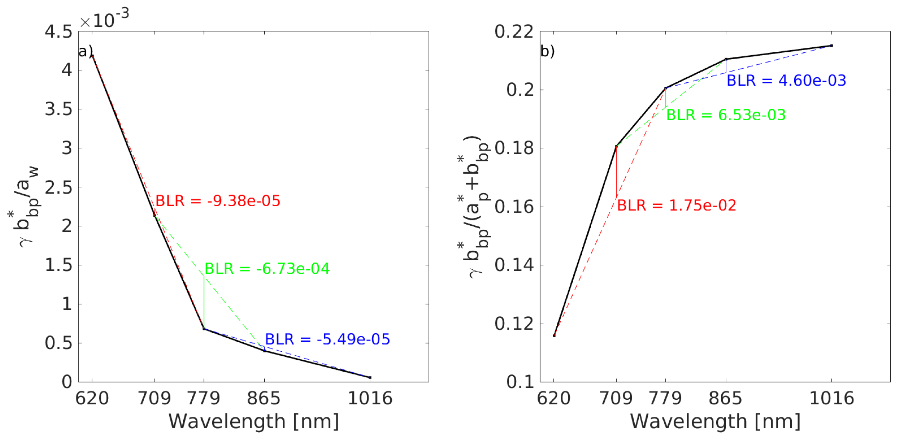
Consider the following expression for the total reflectance at TOA (cf. Gordon and Wang 1994, Equation (1) [1]):

$${\rho }^{TOA}=\pi \frac{L^{TOA}{d}^2}{E^{TOA}cos\left({\theta }_s\right)}$$

(3)

where $L^{TOA}$ is the total radiance at TOA, d the Sun-Earth distance in Astronomical Units, $E^{TOA}$ is the solar extraterrestrial irradiance at TOA and ${\theta }_s$ is the solar zenith angle. A first step common to all atmospheric correction schemes is to estimate the Rayleigh-corrected reflectance (${\rho }_{RC}$), which is obtained by subtracting the path radiance expected from a pure Rayleigh atmosphere with black sea (${\rho }_R$) produced by air molecules from the total signal at TOA, Mobley et al., 2016 [31]:

$${\rho }_{RC}={\rho }^{TOA}-{\rho }_R$$

(4)

The aerosol correction scheme presented here is based on a pixel-by-pixel approach called here baseline residual (BLR), which is the difference between the signal at a “middle” (M) band (i.e., of intermediate wavelength in a triplet of bands) and the value of the baseline formed by the signals at the left (L) and right (R) bands at this middle wavelength, as illustrated in Figure 2. In this work, we use BLRs computed using Rayleigh-corrected (RC) reflectances, so we define $BLR\left({\rho }_{RC}\right)$ as follows:

$$BLR\left({\rho }_{RC}\right)({\lambda }_L,{\lambda }_M,{\lambda }_R)={\rho }_{RC}\left({\lambda }_M\right)-BL\left({\rho }_{RC}\right)\left({\lambda }_M\right|{\lambda }_L,{\lambda }_R)$$

(5)

where ${\lambda }_L$, ${\lambda }_M$ and ${\lambda }_R$ stands for the left, middle and right wavelength of the triplet, ${\rho }_{RC}\left({\lambda }_M\right)$ is the RC reflectance at ${\lambda }_M$ and $BL\left({\rho }_{RC}\right)\left({\lambda }_M\right|{\lambda }_L,{\lambda }_R)$ is the baseline term, given by:

$$BL\left({\rho }_{RC}\right)\left({\lambda }_M\right|{\lambda }_L,{\lambda }_R)=\frac{{\rho }_{RC}\left({\lambda }_L\right)({\lambda }_R-{\lambda }_M)+{\rho }_{RC}\left({\lambda }_R\right)({\lambda }_M-{\lambda }_L)}{{\lambda }_R-{\lambda }_L}$$

(6)

Other precursor algorithms in the ocean colour field that use BLRs, include the fluorescence line height (FLH [15]), defined for MODIS as the BLR of the normalized water-leaving radiances at bands 665 nm, 677 nm and 746 nm, i.e., $FLH=BLR\left(n{L}_w\right)(665,677,746)$; the floating algal index (FAI, Hu 2009 [39]), defined also for MODIS as the BLR of Rayleigh-corrected reflectances at 645 nm, 859 nm and 1240 nm, i.e., $FAI=BLR\left({\rho }_{RC}\right)(645,859,1240)$, the maximum chlorophyll index for MERIS (MCI, Gower and King 2008 [40]), which can be expressed as $MCI=BLR\left(L_{TOA}\right)(681,709,754)$, or the synthetic chlorophyll index (SCI, Shen et al., 2010 [19]), which is computed using remote-sensing reflectances as $SCI=-BLR\left(R_{rs}\right)(620,665,681)-BLR\left(R_{rs}\right)(560,620,681)$ (these bands correspond to the cases of MERIS and OLCI). In some cases these approaches (FLH, SCI) are implemented after an aerosol correction, while in other cases (FAI, MCI) no aerosol correction is applied. Nevertheless, all such approaches are similar in the sense that BLR indexes are essentially unaffected by undesirable signal such as aerosol and/or moderate sun glint (and hence also to typical errors in the process of removal of this signal), since these components are generally spectrally smoother than the in-water signal, especially in the RNS region. Mathematically, if we consider the atmospheric signal “${\rho }_{atm}$” inside the spectral range determined by the band triplet $({\lambda }_L,{\lambda }_M,{\lambda }_R)$ to be as “smooth” as possible, i.e., of linear wavelength dependence, ${\rho }_{atm}\left(\lambda \right)=m\lambda +b$, then $BLR\left({\rho }_{atm}\right)({\lambda }_L,{\lambda }_M,{\lambda }_R)=0$.

The atmospheric correction algorithm presented here was designed taking into consideration that the dependence of BLRs on atmospheric components is best minimized by computing BLRs from RC reflectances at spectrally-close bands, and for longer wavelengths ($\lambda >600$ nm), to reduce the impact of uncertainties in Rayleigh correction, including coupled aerosol-Rayleigh scattering (see Section 2.5 for further reasons). This can be illustrated by considering the following decomposition of RC reflectance, (cf. Gordon and Wang 1994, Equation (2) [1]):

$${\rho }_{RC}\left(\lambda \right)={\rho }_a\left(\lambda \right)+T\left(\lambda \right){\rho }_g+t\left(\lambda \right){\rho }_w\left(\lambda \right)$$

(7)

where each term accounts for photons that arrive at the sensor after: having interacted with aerosols or with both aerosols and molecules (expressed in a summarized form as ${\rho }_a$); being specularly reflected by the water surface (sunglint) ($T\left(\lambda \right){\rho }_g$, where $T\left(\lambda \right)$ is the direct atmospheric transmittance), and having interacted with the in-water components ($t\left(\lambda \right){\rho }_w\left(\lambda \right)$, where $t\left(\lambda \right)$ is the diffuse atmospheric transmittance). Based on typical aerosol types and concentrations such as the modes reported by the World Meteorological Organization (WMO) [29], or by Shettle and Fenn 1979 [41], aerosol reflectances can, in most cases, be modelled as exponential functions of wavelength if considering a sufficiently short bandwidth (see Gordon and Wang 1994 [1], Figure 1):

$${\rho }_a\left({\lambda }_{i=L,M,R}\right)\approx {\rho }_a\left({\lambda }_L\right)e^{-c\frac{{\lambda }_i-{\lambda }_L}{{\lambda }_L}}$$

(8)

where c is related to the aerosol type and ${\rho }_a\left({\lambda }_L\right)$ is the amplitude at ${\lambda }_L$. Typically (but not always) $c>0$, describing a monotonically decreasing wavelength dependence. In particular, in a sufficiently short spectral range, e.g., 250 nm in the RNS, the aerosol reflectance can be approximated as a linear function of wavelength, at least compared to the stronger spectral variability of turbid water reflectance:

$${\rho }_a\left({\lambda }_L\right)e^{-c\frac{{\lambda }_i-{\lambda }_L}{{\lambda }_L}}\approx {\rho }_a\left({\lambda }_L\right)\left(1-c\frac{{\lambda }_i-{\lambda }_L}{{\lambda }_L}\right)$$

(9)

If Equation (9) holds for the spectral range involved in the calculation of BLR (i.e., from ${\lambda }_L$ to ${\lambda }_R$), the aerosol term does not contribute to $BLR\left({\rho }_{RC}\right)({\lambda }_L,{\lambda }_M,{\lambda }_R)$, i.e.,: $BLR\left({\rho }_a\right)({\lambda }_L,{\lambda }_M,{\lambda }_R)\approx 0$ Finally, the sunglint term, at least in a moderate regime, is essentially a white term, especially in short spectral ranges in the RNS region, where we can consider $\frac{\partial T\left(\lambda \right)}{\partial \lambda }\approx 0$, i.e., negligible contribution to $BLR\left({\rho }_{RC}\right)$. Thus, considering any triplet of spectrally close bands in the RNS implies a near-linear spectral dependence of the atmospheric-interface terms in the RC reflectance decomposition. Thus the $BLR\left({\rho }_{RC}\right)$ depends mainly on the in-water term:

$$BLR\left({\rho }_{RC}\right)({\lambda }_L,{\lambda }_M,{\lambda }_R)\approx BLR\left(t{\rho }_w\right)({\lambda }_L,{\lambda }_M,{\lambda }_R)$$

(10)

2.5. Band Choice

In this study, we have chosen to use the RC reflectances computed from the OLCI bands at 620, 709, 779, 865 and 1016 nm. These 5 bands span a ${\mathbb{R}}^5$ space, from which we obtained three successive linearly-independent BLRs: $BLR\left({\rho }_{RC}\right)(620,709,779)$, $BLR\left({\rho }_{RC}\right)(709,779,865)$ and $BLR\left({\rho }_{RC}\right)(779,865,1016)$. These bands have been chosen in order to i) maximize the impact of the (turbid) water signal on $BLR\left({\rho }_{RC}\right)$, and simultaneously ii) minimize the impact of the atmospheric components. Other OLCI bands inside this spectral region were not considered, e.g., those in the range 760–770 nm and the band centered at 940 nm, as they are strongly affected by absorption of atmospheric components such as $O_2$ (oxygen) and $H_{2}Ov$ (water vapour). OLCI bands in the range 660–690 nm are also avoided because the water reflectances there can be affected by chlorophyll absorption and fluorescence.

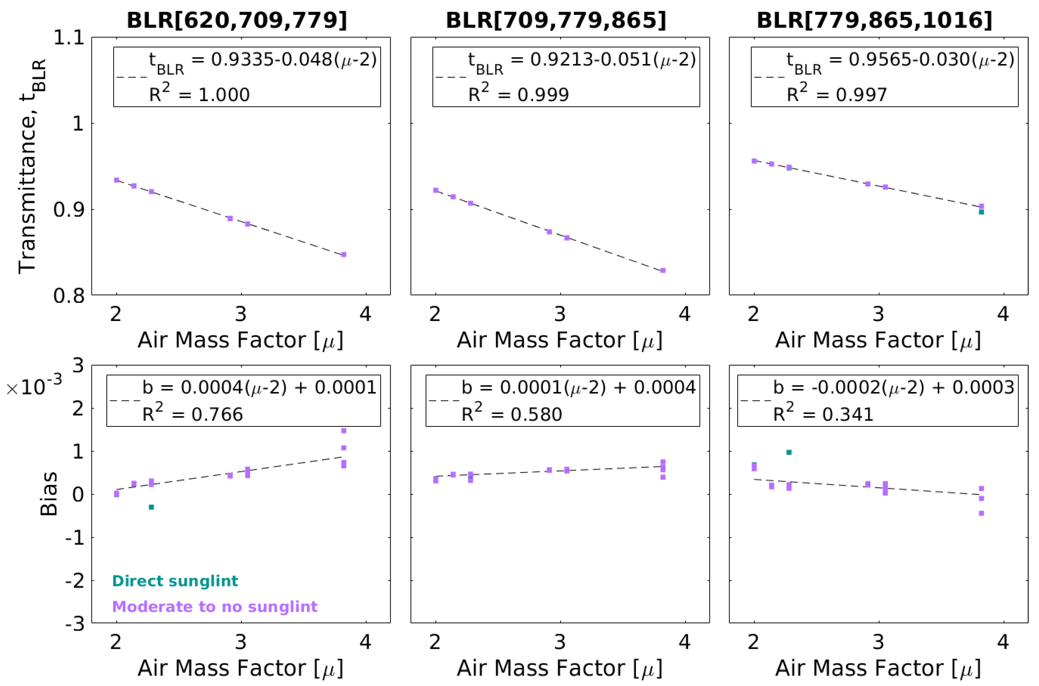
2.6. Transmittance Factor Treatment

The diffuse transmittance factor in Equation (10), accounts for the fact that photons may interact with atmospheric constituents on the path from sun to water and/or from water to sensor. Since it is a second order correction factor, we will assume an equivalent spectrally white diffuse transmittance inside each band triplet, whose expression might depend on geometric conditions and aerosol properties, i.e., as an approximation of Equation (10):

$$BLR\left(t{\rho }_w\right)({\lambda }_L,{\lambda }_M,{\lambda }_R)\approx t_{BLR}({\theta }_s,{\theta }_v,\Delta \varphi ,AER)BLR\left({\rho }_w\right)({\lambda }_L,{\lambda }_M,{\lambda }_R)$$

(11)

where ${\theta }_s$ and ${\theta }_v$ account for the solar and sensor zenith angles, resp.; $\Delta \varphi$ is the sun-sensor azimuth angle difference, and $AER$ stands for the dependence on aerosol type and concentration. Generally, we expect $t_{BLR}$ to be less than (but close to) unity.

To show how the atmosphere affects BLRs computed from the selected bands, Figure 3 shows the relation between $BLR\left({\rho }_w\right)$ computed from in situ measurements, (applying OLCI spectral response functions [42] and Equation (5)) and the corresponding $BLR\left({\rho }_{RC}\right)$, calculated from simulations made with the CNES-SOS radiative transfer code (see Section 2.2, Table 1). In Figure 3b–d, for each $BLR\left({\rho }_w\right)$ computed from the associated input water reflectance, a vertical line (inter-percentile range between percentiles 5 and 95, IPR(5,95)) is shown together with the extreme values (represented by “*”), corresponding to the set of computed RC reflectances for the combination of all possible atmospheric conditions described in Table 1. As a general rule, $BLR\left({\rho }_{RC}\right)$ tend to present lower absolute values than $BLR\left({\rho }_w\right)$, as suggested by the slopes of the linear regressions (i.e., $m<1$). In terms of spectral shape, lower absolute BLRs are associated with spectrally smoother signals, which is consistent with an equivalent transmittance factor smaller than 1 (see Equations (10) and (11)). All scenarios associated to the min/max values, represented by “*”, correspond to cases where the sensor is positioned at reciprocal angles from the sun (i.e., direct sun glint). Apart from these exceptional cases, the low offsets computed for the linear regressions (b), are consistent with the assumptions taken to reach Equation (10), i.e., $BLR({\rho }_a+T{\rho }_g)\approx 0$.

It was observed, from the whole set of simulations, that the dependence of $t_{BLR}$ on the geometric conditions could be reduced to a single variable, the air mass factor, $\mu =\frac{1}{cos\left({\theta }_s\right)}+\frac{1}{cos\left({\theta }_v\right)}$, since, except for the cases of direct sun glint, the relative azimuth was observed to have a very small effect on $t_{BLR}$. This fact is well illustrated in Figure 4, where $t_{BLR}$ and a bias are plotted vs. the air mass factor $\mu$ considering the following expression:

$$BLR\left({\rho }_{RC}\right)=t_{BLR}\left(\mu \right)BLR\left({\rho }_w\right)+bias\left(\mu \right)$$

(12)

In Figure 4, each point represents the result of $t_{BLR}$ (upper insets) and bias (lower insets) of a linear regression of the form of Equation (12) done over subsets defined by a specific set of values for ${\theta }_s$, ${\theta }_v$ and $\Delta \varphi$, i.e., for specific geometric conditions. It can be observed that: (i) biases are usually smaller than $0.001$, and will be neglected in the overall correction for transmittance, and (ii) the dependence of $t_{BLR}$ on $\mu$ can be considered linear in the range $\mu \in [2;4]$. Similar results are observed for increasing aerosol optical thicknesses.

On the basis of these results, the BLRs computed over RC OLCI scenes used to estimate the water signal are divided by the corresponding equivalent transmittance factors for each pixel (Figure 4), to estimate the BLRs from OLCI that will be associated to the water signal in OLCI scenes, i.e.,:

$$BLR\left({\rho }_{w,OLCI}\right):=\frac{BLR\left({\rho }_{RC,OLCI}\right)}{t_{BLR}\left(\mu \right)}$$

(13)

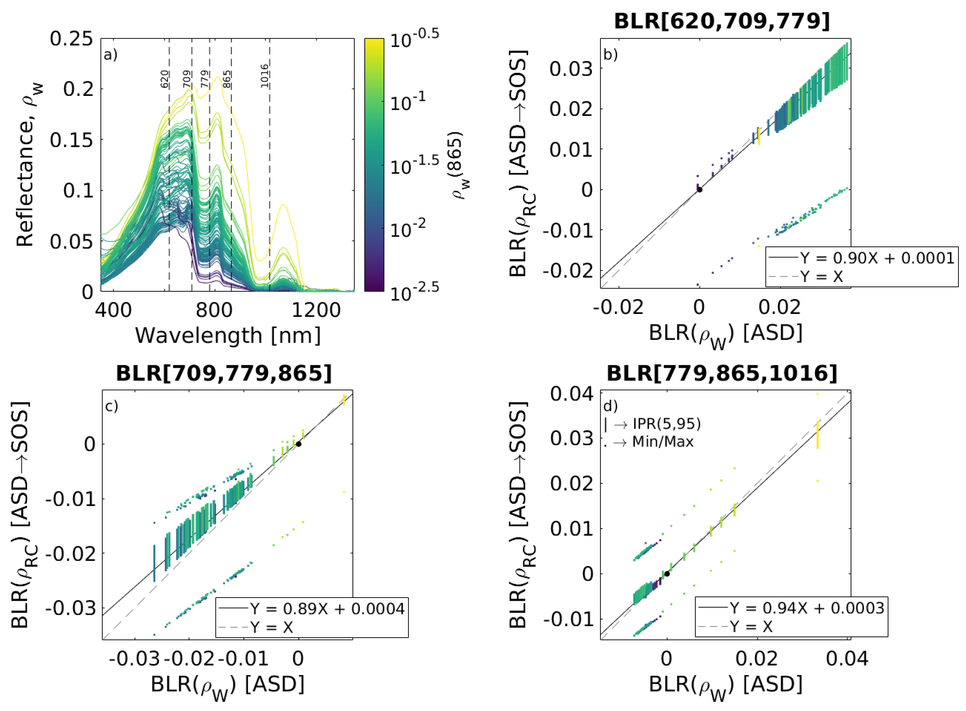
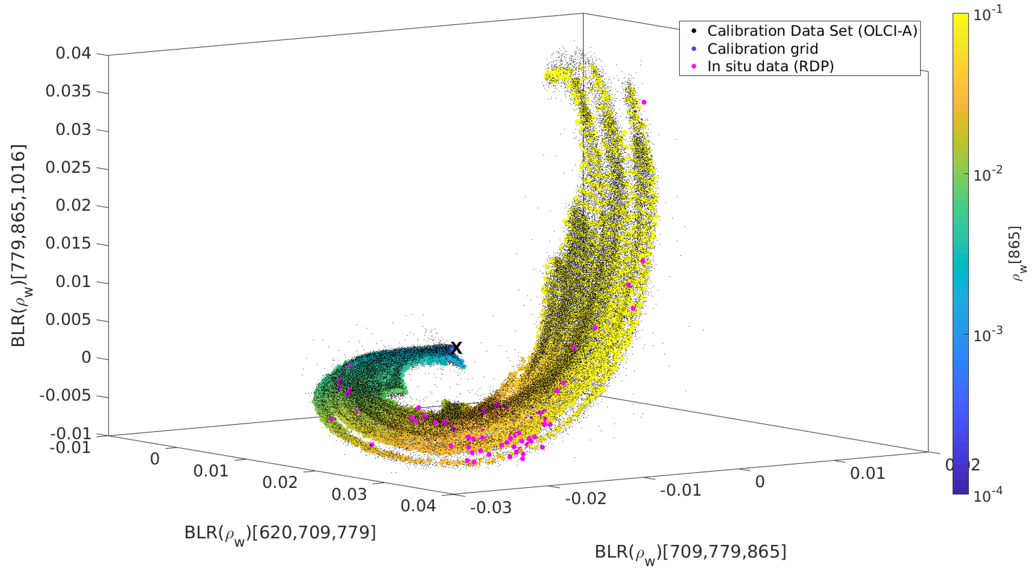
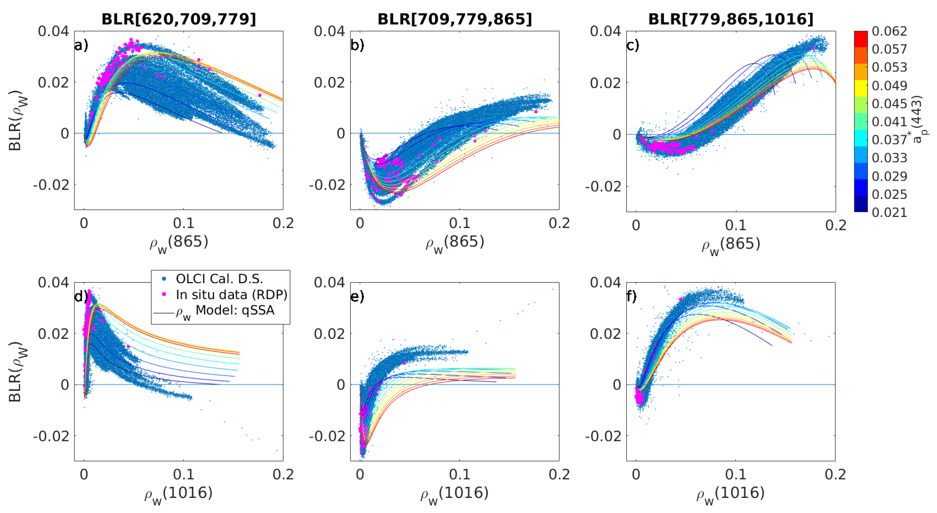
2.7. Relation between Baseline Residuals and Water Reflectances

The previous sections described how $BLR\left({\rho }_w\right)(620,709,779)$, $BLR\left({\rho }_w\right)(709,779,865)$ and $BLR\left({\rho }_w\right)(779,865,1016)$ (Equations (5), (10) and (11)) represent a convenient set of quantities to estimate water reflectance at any of the considered bands. In this study, we focused on establishing a relation between the BLRs and water reflectances of at least two bands: 865 nm and 1016 nm; since this is the minimum required to eventually extrapolate the atmospheric signal to shorter wavelengths. We decided to use a subset of OLCI imagery to achieve a plausible calibration dataset, in order to avoid systematic errors induced by calibrating the algorithm with data coming from other sources (such as in situ measurements or radiative transfer simulations). To build this dataset, a total of 13 sub-regions from 9 cloud-, sunglint- and haze-free scenes were selected from Río de la Plata (see Table 2, magenta boxes at Figure 5). Over these subregions a non-operational atmospheric correction was applied to infer water reflectance at bands 865 nm and 1016 nm, based on estimating the atmospheric component from manually selected fixed clear water windows, close to the windows of interest, of $15\times 15$ pixels, referred to herein as “Fix-AC” (see Table 2, white boxes at Figure 5), and assuming horizontally homogeneous aerosols.

These “clear windows” were chosen to be as close as possible to the subregion of interest and totally free from water signal in the RNS (determined by visual inspection of the ${\rho }_{RC}$ rasters). This simple aerosol removal assumes a spatially uniform atmospheric signal which is subtracted from the whole subregion of interest as follows:

$${\rho }_w=\frac{{\rho }_{RC}-{\rho }_a^{ClearWin}}{t(\lambda ,\mu )}$$

(14)

where a simple expression is used for the two-way transmittance factor, $t(\lambda ,\mu )$, (as applied by NASA OBPG in the absence of aerosol information and molecular absorption, Mobley et al., 2016 [31]) which depends on the air mass factor, $\mu$, (see Section 2.6) and the Rayleigh optical thickness, ${\tau }_{Ray}\left(\lambda \right)$ (Bodhaine et al., 1999 [30]):

$$t(\lambda ,\mu )=e^{-\frac{0.5{\tau }_{Ray}\left(\lambda \right)}{cos\left({\theta }_s\right)}}{e}^{-\frac{0.5{\tau }_{Ray}\left(\lambda \right)}{cos\left({\theta }_v\right)}}=e^{-0.5{\tau }_{Ray}\left(\lambda \right)\mu }$$

(15)

Once this process is performed, the calibration dataset formed by the mentioned subregions is used to fit a calibration surface in BLR 3-dimensional sub-space, which is spanned by $BLR(620,709,779)$, $BLR(709,779,865)$ and $BLR(779,865,1016)$ (see Figure 5 and Figure 6). The calibration surface is generated by binning on a 2-dimensional mesh-grid of “X” ($BLR(620,709,779)$) in the range $(-0.0100;0.0350)$ (step $0.0005$) and “Y” ($BLR(709,779,865)$) in the range $(-0.0300;0.0150)$ (step $0.0005$). The “Z” ($BLR(779,865,1016)$) values at each point of the grid are taken as the median of the Z values taken by the calibration dataset in the corresponding $(X,Y)$ pair. This can be done in this way since the BLR surface does not present ambiguity in Z, i.e., the BLR surface can be considered as a function of $(X,Y)$: $Z=f(X,Y)$. The calibration point is discarded if less than 10 data fall inside the associated $(X,Y)$ range.

The $BLRs\left({\rho }_w\right)$ triplet computed at each input pixel is associated to the closest (in the Euclidean sense) $BLRs\left({\rho }_w\right)$ triplet that corresponds to the calibration curve, and the corresponding water reflectance at 865 nm and 1016 nm is assigned to the given pixel.

2.8. Estimation of Aerosol Reflectance at Bands 865 nm and 1016 nm

The aerosol reflectance, ${\rho }_a$, at 865 and 1016 nm is computed to test the spatial correlation with the estimated marine signal -which is expected to be low- using the following simplified expression:

$${\rho }_a\left(\lambda \right)={\rho }_{RC}\left(\lambda \right)-t(\lambda ,\mu ){\rho }_{w,j}\left(\lambda \right)$$

(16)

where ${\rho }_{w,j}$ is the water reflectance value assigned to the nearest Euclidean neighbour from the calibrations surface at the BLR space. The transmittance factor is calculated in the same way as in Equation (15). This same expression was applied to intercompare with the aerosol reflectances yielded by other preexistent schemes (BAC/BPAC and SeaDAS-2 (865, 1016)). A last correction is performed on ${\rho }_a\left(865\right)$ to restrain the derived ${ϵ}_a(865,1016)=\frac{{\rho }_a\left(865\right)}{{\rho }_a\left(1016\right)}$ inside the range of $(0.85;1.25)$. These bounds were determined as the extreme values taken over a set of 82 different selected windows of size $15px\times 15px$ from OLCI-A scenes of clear water regions close to Río de la Plata, Bahía Blanca, North Sea, Yellow Sea, Amazonas and North Australia. Also these bounds are consistent with what was obtained over the CNES-SOS simulations. This correction is performed by imposing the following condition on a pixel-by-pixel basis:

$$0.85{\rho }_a\left(1016\right)\le {\rho }_{a,new}\left(865\right)\le 1.25{\rho }_a\left(1016\right)$$

(17)

and then, consequently correcting the retrieved ${\rho }_w\left(865\right)$ values. This constraint is further discussed in Section 4.

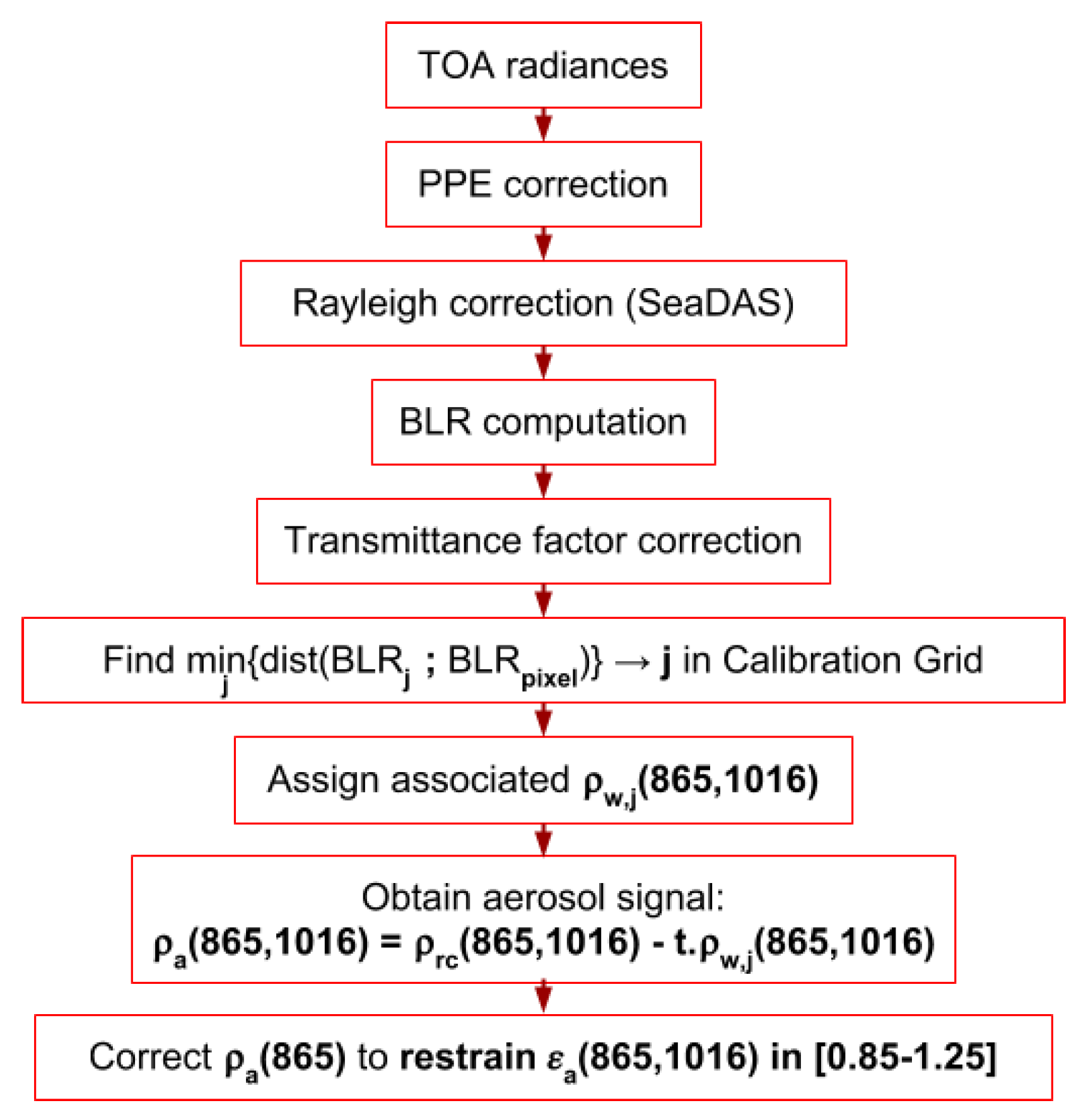
2.9. Atmospheric Correction Scheme: Summary

The following list (shown in Figure 7) summarizes the atmospheric correction algorithm developed in this study:

• The PPE correction (Gossn 2018 [34]) is applied on L1B imagery (TOA radiances).
• Rayleigh (and gaseous absorption) correction is applied using SeaDAS v7.5 software.
• $BLR\left({\rho }_{RC}\right)(620,709,779)$, $BLR\left({\rho }_{RC}\right)(709,779,865)$ and $BLR\left({\rho }_{RC}\right)(779,865,1016)$ are computed from the corresponding Rayleigh-corrected reflectances (see Section 2.4 and Section 2.5, Equation (5)).
• A transmittance factor correction is applied to relate $BLR\left({\rho }_{RC}\right)$ with $BLR\left({\rho }_w\right)$ (see Section 2.6, Equation (13)).
• For each pixel, the computed BLRs are matched to the BLRs from the calibration surface that minimize the Euclidean distance in BLR space. The corresponding water reflectance at 865 nm and 1016 nm is assigned to the pixel (see Section 2.7).
• The atmospheric residual at these bands is obtained by subtracting the assigned water signal to the RC reflectance (see Section 2.8, Equation (16)).
• A final constraint is applied to ${\rho }_a\left(865\right)$ to limit ${ϵ}_a(865,1016)$ inside the reasonable range of $(0.85;1.25)$ (see Section 2.8, Equation (17)).

This approach may be extended to the whole range of bands of interest by subtracting the water signal retrieved and applying the clear pixel assumption to extrapolate the aerosol signal to shorter wavelengths (Gordon and Wang 1994 [1], Stumpf et al., 2003 [2]).

3. Results

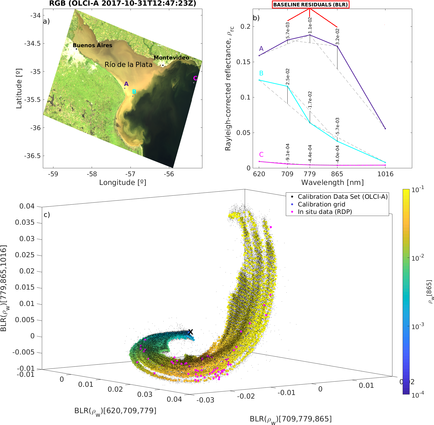
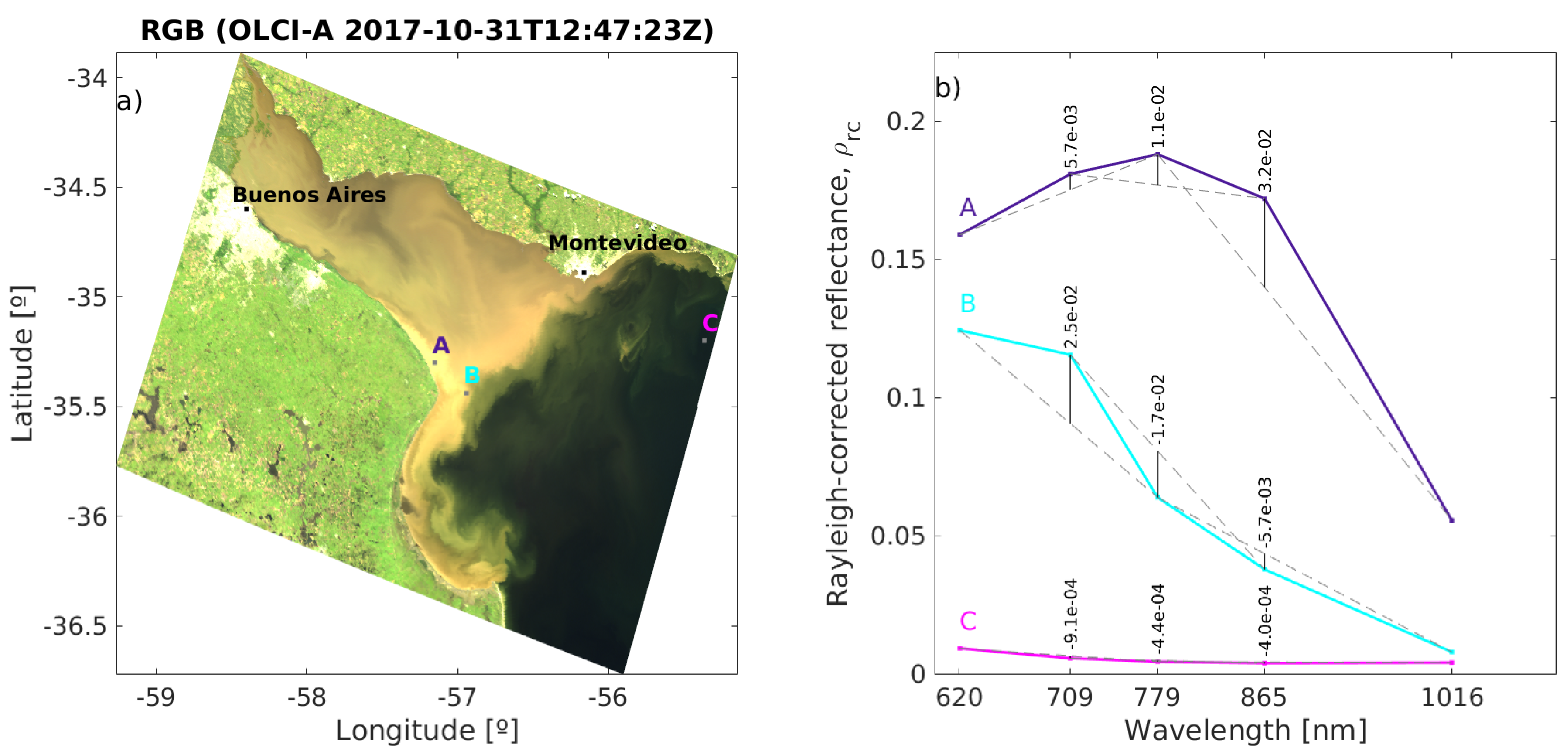
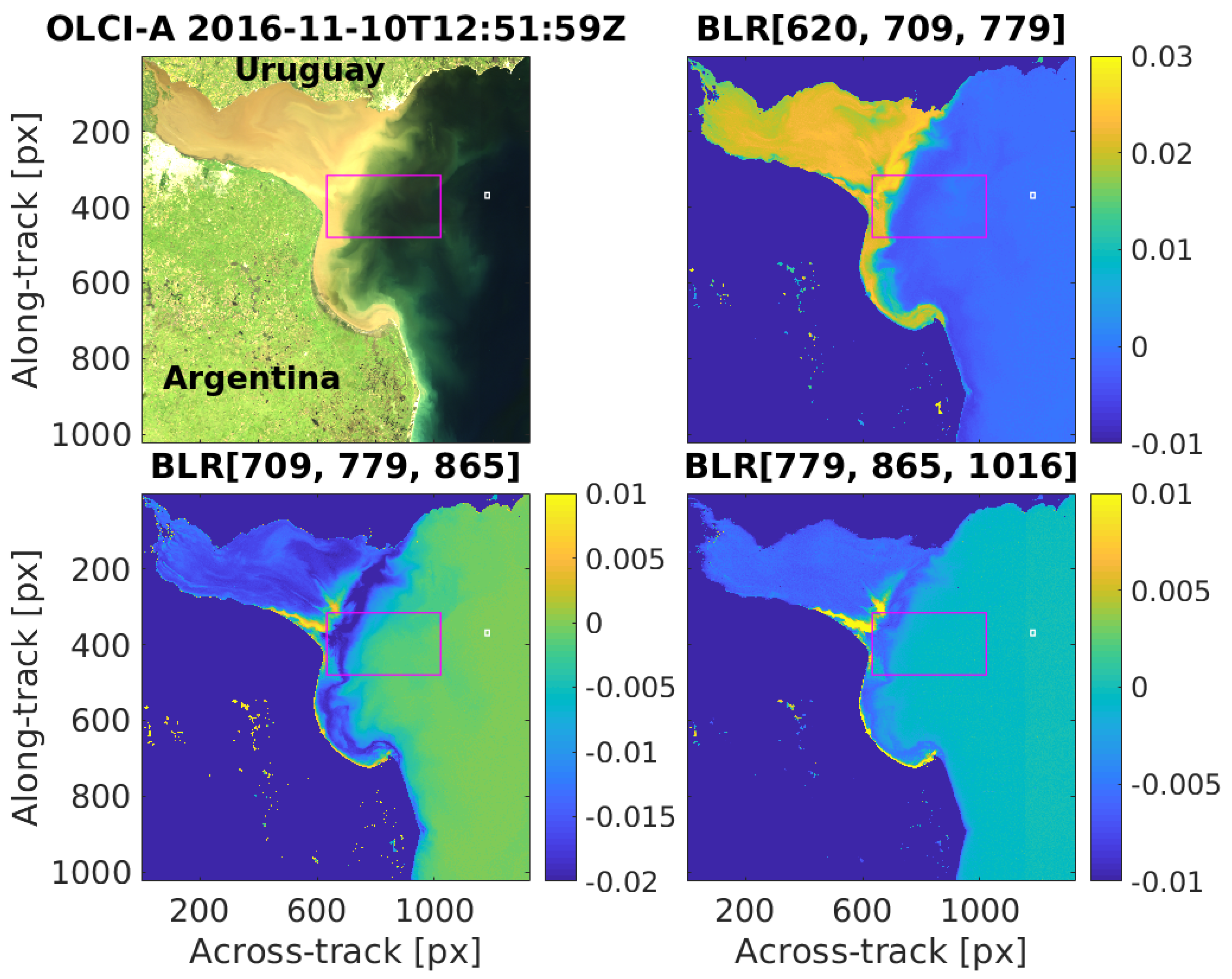
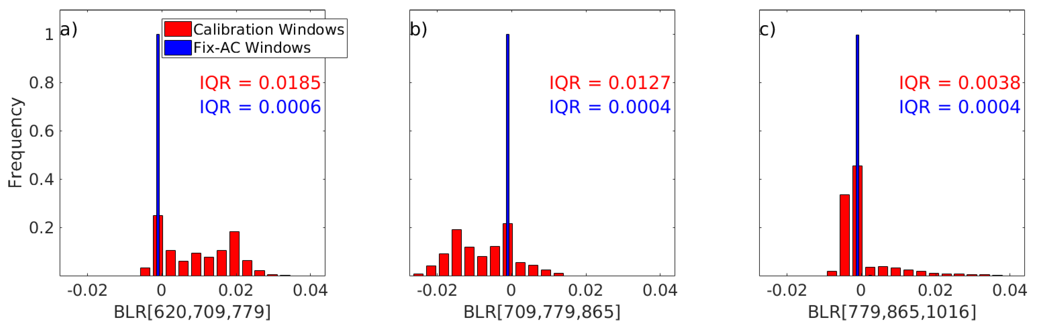
3.1. Baseline Residuals in Clear and Turbid Waters

The fact that BLRs of the considered triplets approach near-zero values in clear waters is expressed through Equation (10), assuming that very clear waters appear as black in the RNS. This property is clearly seen from OLCI RC reflectances, and is evident from Figure 8 (as well as Figure 2 and Figure 5), where BLR distributions are intercompared from OLCI scenes from (i) windows selected to perform the BLR-AC calibration (which contain mainly turbid waters, calibration windows in Table 2), and (ii) windows selected to perform the Fix-AC scheme (which contain very clear waters, Fix-AC windows in Table 2). It is clearly seen from Figure 8 that BLR mean values and interquartile ranges (IQR) over the Fix-AC windows are close to 0 (always smaller than ${10}^{-3}$) and the Fix-AC window IQR are at least 9 times smaller than the computed IQRs for the calibration windows. This is in accordance with what has been predicted and shows that for this approach the black water condition is translated to the condition $BLR\left({\rho }_w\right)=0$ (also evident by observing the clear water regions at Figure 5). This means that, given a pixel where simultaneously $BLR\left({\rho }_w\right)=0$ for the three considered triplets, the algorithm yields ${\rho }_w\left(865\right)={\rho }_w\left(1016\right)=0$, i.e., the algorithm returns naturally to the standard AC approach for clear waters.

This is also evident from Figure 9, where three different sources of the $BLR$ vs. ${\rho }_w$ relation are intercompared to show how the baseline residuals at each of the three considered triplets of wavelengths vary according to water reflectances at 865 nm and 1016 nm. Blue dots show data from the calibration windows (Table 2); in magenta, BLRs computed from in situ data collected from Río de la Plata (Section 2.1), and a family of colour-mapped curves show the $BLR$ vs. ${\rho }_w$ relation using a quasi-single scattering approximation (qSSA) reflectance model, described in Appendix A, where all specific IOPs, except specific particle absorption at a fixed wavelength (443 nm), were fixed in ranges consistent with previous publications (cf. Luo et al., 2018, Table 1 [7]) and where SPM varied logarithmically between $0.001{\mathrm{g}/\mathrm{m}}^3$ and 10,000 ${\mathrm{g}/\mathrm{m}}^3$.

Although there is an evident high resemblance between the three sources, it must be noticed that the qSSA curves depart from (remotely and in situ) measured water reflectances mainly because the underlying analytical reflectance model is less reliable at high reflectance (see Appendix A). The variations over the BLR vs. ${\rho }_w$ relation observed between the different qSSA curves indicate that BLRs might be very sensitive to particle absorption; which means that they might be used as indicative of different specific optical properties of particles in highly turbid waters. Nonetheless, this hypothesis must be ascertained with simultaneous reflectance and particle absorption field data, to test and validate optical closure, in the same way as expressed in Luo et al., 2018 [7].

In the three triplets considered, modelled $BLR\left({\rho }_w\right)$ behave similarly with increasing reflectance. At ${\rho }_w=0$, they all approach values towards 0, recovering the black water condition $BLR({\rho }_w=0)=0$ seen in Figure 8. As reflectances increase, BLRs take negative values, which can be understood if we consider ${\rho }_w\propto \frac{b_{b,p}^{*}}{a_w}$ for very low turbidities (low sediment content) (cf. Ruddick et al., 2006, Equation (14) [5]). Given the simple qSSA reflectance model described in Appendix A, with specific IOPs taken from reported values in Babin et al., 2003 (a and b) [43,44], this magnitude is convex for the considered OLCI bands, i.e., negative BLRs (Figure 10a). On the contrary, for very high turbidities, water reflectances tend to achieve a constant value (saturation) that depends on the specific IOPs of the particulate content of the water: ${\rho }_w\propto \frac{b_{b,p}^{*}}{a_p^{*}+b_{b,p}^{*}}$ (cf. Dogliotti et al., 2015, Equation (A2) [16]). In this case, this magnitude is concave for the considered OLCI bands in the qSSA relfectance model, i.e., positive BLRs (Figure 10b).

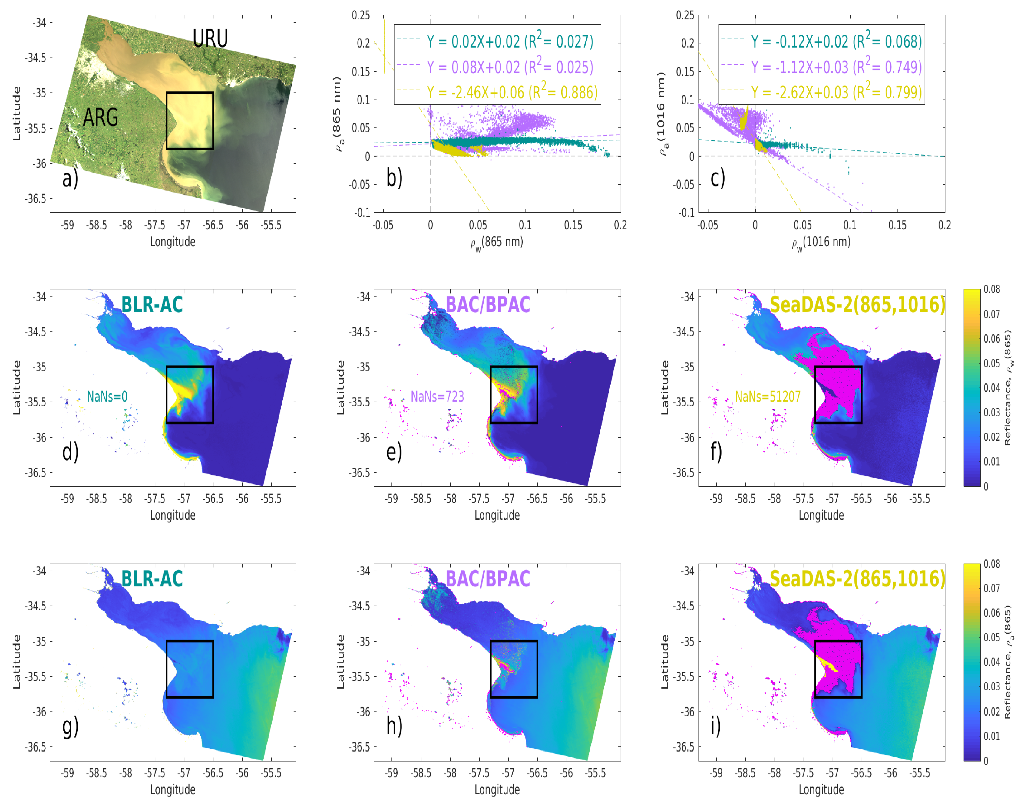
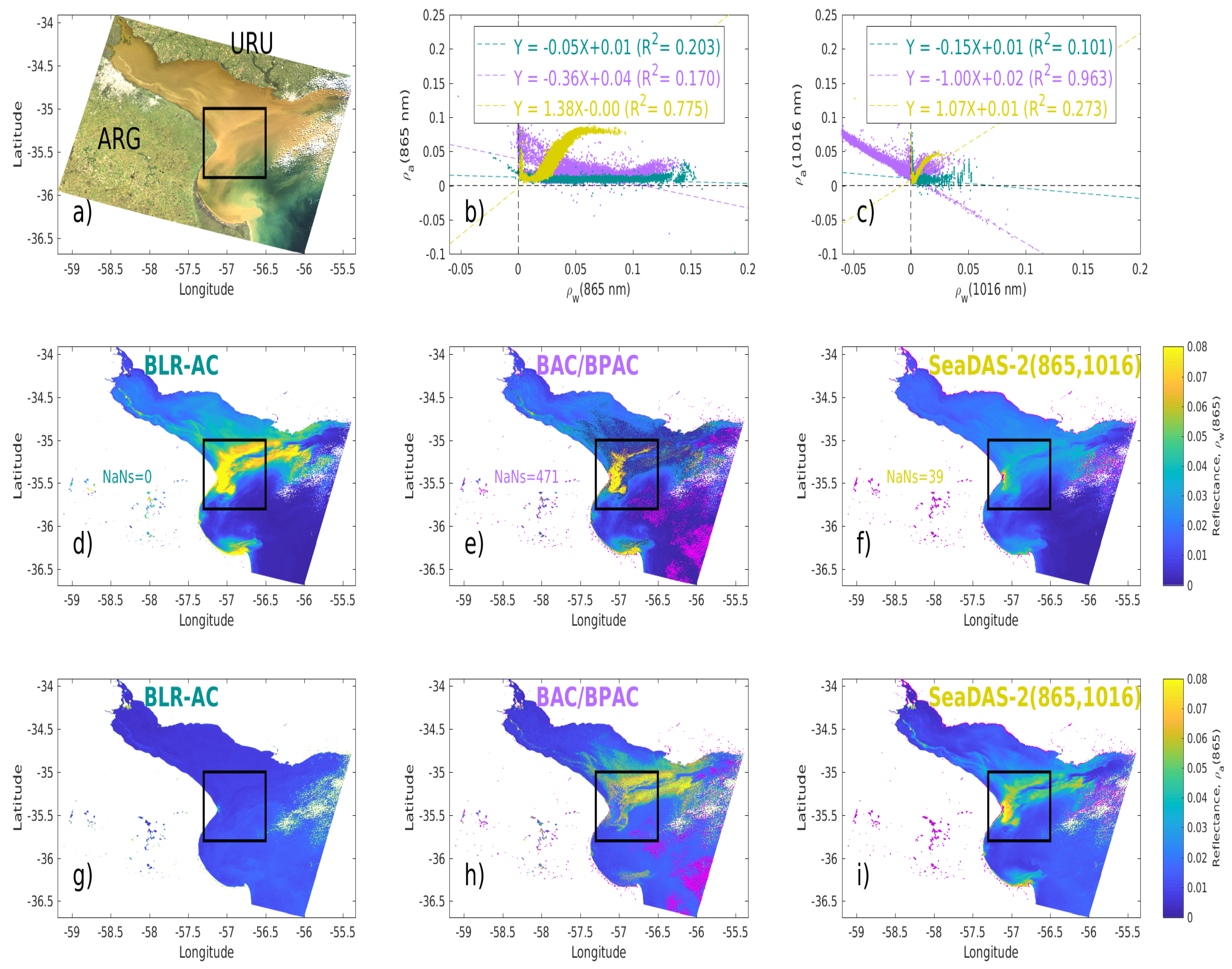
3.2. Atmospheric Correction Performance

Given the lack of match-ups between in situ measurements and OLCI data for the studied regions (or any other extremely turbid waters), the Fix-AC approach (considered to be of high performance for the chosen scenes but not appropriate for a global automated processor) was used as a reference to validate the performance of the automated BLR-AC scheme (Figure 11). Pixels inside the marked coloured boxes, corresponding to the most turbid parts of the validation images listed in Table 2 were selected. The three regions were selected as representative of extremely turbid (Figure 11b) and moderately turbid (Figure 11a,c) waters. Water reflectances derived from both approaches show very similar patterns and very small root mean square difference (RMSD) values in both cases. In the case of the 620 nm band, ${\rho }_w^{BLR-AC}$ values were obtained by using a simple linear aerosol extrapolation from the correction bands at 865 and 1016 nm.

Another way of evaluating the performance of an atmospheric correction is through the analysis of the spatial (de)correlation between the retrieved water and aerosol reflectances. Figure 12, Figure 13 and Figure 14 show water and aerosol reflectances at 1016 nm retrieved by BLR-AC from OLCI scenes over Río de la Plata (2017-01-21T13:24:42Z, 2016-06-08T13:09:51Z, 2017-12-12T12:59:01Z, Table 2), together with standard atmospheric corrections: ESA’s BAC/BPAC and NASA’s SeaDAS-2 (865, 1016) (see Section 2.3). The most challenging region for atmospheric correction over RdP is the turbidity front adjacent to Buenos Aires Province Coast (Argentina) at around 35°5 S; 57°0 W (marked as $0.8°\times 0.8°$ black boxes), where SPM, turbidity and water reflectances at the RNS are maximum [8,24]. It is evident from the higher slopes and $R^2$ values retrieved by linear regressions in Figure 12b,c how standard atmospheric corrections yield higher (unphysical) correlation between the water and aerosol signals. This is also evident by visually comparing the water and aerosol rasters in the BLR-AC case, compared to BAC/BPAC and SeaDAS-2 (865, 1016). In general terms, BAC/BPAC and SeaDAS-2 (865, 1016) underestimate water signal or simply do not converge to a numeric solution (i.e., NaNs, seen as magenta in Figure 12e,f,h,i, Figure 13e,f,h,i and Figure 14e,f,h,i). The image shown in Figure 12 is partially contaminated with moderate sunglint (toward the East edge), which is clearly removed as non-water signal for the BLR-AC and BAC/BPAC schemes. The image shown in Figure 14 is partially contaminated with thin clouds. BLR-AC is clearly capable of separating thin cloud from turbid water signal.

4. Discussion

The new atmospheric correction approach presented here has the advantage that it is designed on the basis of clear physical principles and thus highlights (e.g., Figure 6) how factors such as natural variability of specific inherent optical properties of water, TOA satellite data calibration and the choice of spectral bands may impact algorithm performance. BLRs computed from in situ measurements and OLCI data behave in a similar way and in accordance with a quasi-single scattering approximation (qSSA) reflectance model, although the qSSA model departs from measured reflectances at extreme turbidities, because of the underlying qSSA approximations (Figure 9).

While the new algorithm already gives a good performance for retrieval of Red/NIR/SWIR water reflectance, particularly in extremely turbid waters, and can thus be used directly for estimation of turbidity, SPM and chlorophyll-a concentration (in turbid waters using Red/NIR algorithms), further improvements may be necessary for retrieval of water reflectance at shorter wavelengths in turbid waters, if the latter is actually needed for subsequent water constituent retrieval algorithms. In extremely turbid waters the Red/NIR Rayleigh-corrected reflectance is dominated by water reflectance and retrieved aerosol reflectances and, in particular, the retrieved aerosol type (through ${ϵ}_a(865,1016)$) can be highly impacted by small errors in the water reflectance estimates—in fact, in this situation it is precisely the water reflectance that can be better estimated in relative terms than the aerosol reflectance. If more reliable ${ϵ}_a(865,1016)$ are required in extremely turbid waters for extrapolation to shorter wavelengths then the current approach could be improved in the future by integration of extra information. For example, extra constraints could be applied to ${ϵ}_a(865,1016)$ by the use of ultraviolet/violet bands (He et al., 2012 [45]) or by spatial smoothing of ${ϵ}_a(865,1016)$ assuming that the horizontal length scale for variation of aerosol type is larger than the pixel size (Ruddick et al., 2000 [46]). In the present study no such horizontal smoothing has been applied, enabling us to better understand the capabilities and limitations of an automated pixel-by-pixel approach and hence identify, for example, the intrinsic value of the various spectral bands in separating aerosol and water reflectance in the RNS and the potential sources of uncertainty in this decomposition. In a future version of the algorithm, the constraint on ${ϵ}_a(865,1016)$ applied at the last step (Section 2.9, step 7) of the processing might be replaced by either or both of these spectral/spatial constraints, and might address BLR optimization with a more refined method.

While the new algorithm relies on a BLR calibration surface (Section 2.9, step 5) constructed with Río de la Plata OLCI imagery, the AC scheme has been also tested in many other sites with sediment-dominated waters, like the Amazonas Plume, Bohai Sea, Belgian Coast, Bahía Blanca, (see Figure 11), using this calibration surface, so we currently consider that it will not be necessary to apply different calibrations to different regions.

5. Conclusions

A new atmospheric correction algorithm for highly turbid waters is presented for S3/OLCI. The key assumption is that the spectral convexity of Rayleigh-corrected reflectance in the RNS is determined by water reflectance and is essentially unaffected by aerosols. This spectral convexity is quantified here through baseline residuals (BLRs, Equation (5)) of the three consecutive triplets of the OLCI bands centered at 620, 709, 779, 865 and 1016 nm. An “equivalent transmittance” applicable to BLRs that depends on the air mass factor was derived from in situ measurements and radiative transfer simulations. The algorithm that relates BLRs to water reflectances at 865 and 1016 nm was calibrated by using OLCI data from selected subregions of images from Río de la Plata (Argentina), which were atmospherically-corrected by a simple fix window atmospheric correction (Fix-AC) that assumes spatial homogeneity of the atmosphere (given very clear sky conditions and small horizontal distances) and computes the atmospheric reflectance from fixed windows corresponding to clear water regions. The performance of the BLR-AC algorithm compares favourably with existing atmospheric correction algorithms (the standard ESA/OLCI processor and the SeaDAS processor implemented with the OLCI 865 nm and 1016 nm bands), particularly in extremely turbid waters, where existing algorithms either fail or show unphysical correlation between aerosol and water reflectance images (Figure 12, Figure 13 and Figure 14). The performance improvement is achieved due to use of multiple red/NIR/SWIR bands, including the new OLCI 1016 nm band, which facilitates separation of water and aerosol reflectances even for extremely turbid waters. Although the BLR approach is designed here for OLCI imagery, it might be easily expandable to other sensors that have spectrally-close triplets of bands in the Red/NIR/SWIR, such as the Argentine-Brazilian joint mission SABIA-Mar, or hyperspectral sensors such as HICO or CHRIS/PROBA.

References

1. Gordon, H.R.; Wang, M. Retrieval of water-leaving radiance and aerosol optical thickness over the oceans with SeaWiFS: A preliminary algorithm. Appl. Opt. 1994, 33, 443–452. [Google Scholar] [CrossRef] [PubMed]
2. Stumpf, R.; Arnone, R.; Gould, R.; Martinolich, P.M.; Ransibrahmanakul, V. A partially coupled ocean-atmosphere model for retrieval of water-leaving radiance from SeaWiFS in coastal waters. NASA Tech. Memo 2003, 206892, 51–59. [Google Scholar]
3. Doxaran, D.; Froidefond, J.M.; Castaing, P. Spectral signature of highly turbid waters: Application with SPOT data to quantify suspended particulate matter concentrations. Remote Sens. Environ. 2002, 81, 149–161. [Google Scholar] [CrossRef]
4. Ruddick, K.; Vanhellement, Q. Use of OLCI and SLSTR Bands for Atmospheric Correction over Turbid Coastal and Inland Waters. In Proceedings of the Sentinel-3 for Science Workshop, Casinò, Italy, 2–5 June 2015; Volume 734, p. 55. [Google Scholar]
5. Ruddick, K.G.; De Cauwer, V.; Park, Y.J.; Moore, G. Seaborne measurements of near infrared water-leaving reflectance: The similarity spectrum for turbid waters. Limnol. Oceanogr. 2006, 51, 1167–1179. [Google Scholar] [CrossRef] [Green Version]
6. Lee, Z.; Shang, S.; Lin, G.; Chen, J.; Doxaran, D. On the modeling of hyperspectral remote-sensing reflectance of high-sediment-load waters in the visible to shortwave-infrared domain. Appl. Opt. 2016, 55, 1738–1750. [Google Scholar] [CrossRef] [PubMed]
7. Luo, Y.; Doxaran, D.; Ruddick, K.; Shen, F.; Gentili, B.; Yan, L.; Huang, H. Saturation of water reflectance in extremely turbid media based on field measurements, satellite data and bio-optical modelling. Opt. Express 2018, 26, 10435–10451. [Google Scholar] [CrossRef]
8. Dogliotti, A.; Ruddick, K.; Nechad, B.; Lasta, C. Improving Water Reflectance Retrieval from MODIS Imagery in the Highly Turbid Waters of La Plata River. In Proceedings of the VI International Conference: Current Problems in Optics of Natural Waters (ONW 2011), St. Petersburg, Russia, 6–10 September 2011; p. 152. [Google Scholar]
9. Wang, M.; Shi, W. Estimation of ocean contribution at the MODIS near-infrared wavelengths along the east coast of the US: Two case studies. Geophys. Res. Lett. 2005, 32, L13606. [Google Scholar] [CrossRef]
10. Knaeps, E.; Dogliotti, A.I.; Raymaekers, D.; Ruddick, K.; Sterckx, S. In situ evidence of non-zero reflectance in the OLCI 1020nm band for a turbid estuary. Remote Sens. Environ. 2012, 120, 133–144. [Google Scholar] [CrossRef]
11. Doerffer, R.; Schiller, H. The MERIS Case 2 water algorithm. Int. J. Remote Sens. 2007, 28, 517–535. [Google Scholar] [CrossRef]
12. Chomko, M.; Gordon, H. Atmospheric Correction of Ocean Color Imagery: Test of the Spectral Optimization Algorithm with the Sea-Viewing Wide Field-of-View Sensor. Appl. Opt. 2001, 40, 2973–2984. [Google Scholar] [CrossRef]
13. Steinmetz, F.; Deschamps, P.Y.; Ramon, D. Atmospheric correction in presence of sun glint: Application to MERIS. Opt. Express 2011, 19, 9783–9800. [Google Scholar] [CrossRef] [PubMed]
14. Philpot, W. The derivative ratio algorithm: Avoiding atmospheric effects in remote sensing. IEEE Trans. Geosci. Remote Sens. 1991, 29, 350–357. [Google Scholar] [CrossRef]
15. Letelier, R.; Abbott, M. An analysis of chlorophyll fluorescence algorithms for the Moderate Resolution Imaging Spectrometer (MODIS). Remote Sens. Environ. 1996, 58, 215–223. [Google Scholar] [CrossRef]
16. Dogliotti, A.; Ruddick, K.; Nechad, B.; Doxaran, D.; Knaeps, E. A single algorithm to retrieve turbidity from remotely-sensed data in all coastal and estuarine waters. Remote Sens. Environ. 2015, 156, 157–168. [Google Scholar] [CrossRef] [Green Version]
17. Dogliotti, A.; Ruddick, K.; Guerrero, R. Seasonal and inter-annual turbidity variability in the Río de la Plata from 15 years of MODIS: El Niño dilution effect. Estuar. Coast. Shelf Sci. 2016, 182, 27–39. [Google Scholar] [CrossRef] [Green Version]
18. Nechad, B.; Ruddick, K.; Park, Y. Calibration and validation of a generic multisensor algorithm for mapping of total suspended matter in turbid waters. Remote Sens. Environ. 2010, 114, 854–866. [Google Scholar] [CrossRef]
19. Shen, F.; Zhou, Y.X.; Li, D.J.; Zhu, W.J.; Salama, M. Medium resolution imaging spectrometer (MERIS) estimation of chlorophyll-a concentration in the turbid sediment-laden waters of the Changjiang (Yangtze) Estuary. Int. J. Remote Sens. 2010, 31, 4635–4650. [Google Scholar] [CrossRef]
20. Moreira, D.; Simionato, C.; Gohin, F.; Cayocca, F.; Luz Clara, M. Suspended matter mean distribution and seasonal cycle in the Rio de La Plata estuary and the adjacent shelf from ocean color satellite (MODIS) and in-situ observations. Cont. Shelf Res. 2013, 68, 51–66. [Google Scholar] [CrossRef]
21. Gilerson, A.A.; Gitelson, A.A.; Zhou, J.; Gurlin, D.; Moses, W.; Ioannou, I.; Ahmed, S.A. Algorithms for remote estimation of chlorophyll-a in coastal and inland waters using red and near infrared bands. Opt. Express 2010, 18, 24109–24125. [Google Scholar] [CrossRef]
22. Gitelson, A. The peak near 700 nm on radiance spectra of algae and water: Relationships of its magnitude and position with chlorophyll concentration. Int. J. Remote Sens. 1992, 13, 3367–3373. [Google Scholar] [CrossRef]
23. Gons, H.J.; Rijkeboer, M.; Ruddick, K.G. Effect of a waveband shift on chlorophyll retrieval from MERIS imagery of inland and coastal waters. J. Plankton Res. 2005, 27, 125–127. [Google Scholar] [CrossRef]
24. Framiñan, M.; Brown, O. Study of the Río de la Plata turbidity front, Part 1: Spatial and temporal distribution. Cont. Shelf Res. 1996, 16, 1259–1282. [Google Scholar] [CrossRef]
25. Mueller, L.J.; Morel, A.; Frouin, R.; Davis, C.; Arnone, R.; Carder, K.; Li, Z.; Steward, R.; Hooker, S.; Mobley, C.; et al. Ocean Optics Protocols for Satellite Ocean Color Sensor Validation, Revision 4, Volume III: Radiometric Measurements and Data Analysis Protocols; Technical Report NASA/TM-2003-21621/Rev-Vol III; NASA Goddard Space Flight Center: Greenbelt, MD, USA, 2003.
26. Mobley, C.D. Estimation of the remote-sensing reflectance from above-surface measurements. Appl. Opt. 1999, 38, 7442–7455. [Google Scholar] [CrossRef]
27. Lenoble, J.; Herman, M.; Deuzé, J.L.; Lafrance, B.; Santer, R.; Tanré, D. A successive order of scattering code for solving the vector equation of transfer in the earth’s atmosphere with aerosols. J. Quant. Spectrosc. Radiat. Transf. 2007, 107, 479–507. [Google Scholar] [CrossRef]
28. Cox, C.; Munk, W. Measurement of the Roughness of the Sea Surface from Photographs of the Sun’s Glitter. J. Opt. Soc. Am. 1954, 44, 838–850. [Google Scholar] [CrossRef]
29. Programme, W.C.R. A Preliminary Cloudless Standard Atmosphere for Radiation Computation; Technical Report WMO/TD, no. 24.; WCP (Series), 112; International Association of Meteorology and Atmospheric Physics: Boulder, CO, USA, 1986. [Google Scholar]
30. Bodhaine, B.A.; Slusser, J.R. On Rayleigh Optical Depth Calculations. J. Atmos. Ocean. Technol. 1999, 16, 1854–1861. [Google Scholar] [CrossRef]
31. Mobley, C.; Werdell, J.; Franz, B.; Ahmad, Z.; Bailey, S. Atmospheric Correction for Satellite Ocean Color Radiometry; Technical report; NASA Goddard Space Flight Center: Greenbelt, MD, USA, 2016.
32. Copernicus Online Data Access. EUMETSAT. Available online: coda.eumetsat.int (accessed on 1 February 2018).
33. S3 Mission Performance Centre (2017), Sentinel-3 Product Notice S3A.PN-OLCI-L2L.02, Issue/Rev Date 06/11/2017. Available online: sentinel.esa.int/documents/247904/2702575/Sentinel-3-OLCI-Product-Notice-Level-2-Land (accessed on 20 November 2017).
34. Gossn, J.I. Effect of Prompt Particle Events on OLCI Ocean Color Imagery in the South Atlantic Anomaly: Detection and Removal. IEEE Geosci. Remote Sens. Lett. 2018. [Google Scholar] [CrossRef]
35. D’Amico, G.; Corsini, M.D.; Nieke, J. Prompt-Particle-Events in ESA’s Envisat/MERIS and Sentinel-3/OLCI Data: Observations, Analysis and Recommendations. Master’s Thesis, University of Pisa, Pisa, Italy, 2015. [Google Scholar]
36. Bailey, S.W.; Franz, B.A.; Werdell, P.J. Estimation of near-infrared water-leaving reflectance for satellite ocean color data processing. Opt. Express 2010, 18, 7521–7527. [Google Scholar] [CrossRef]
37. Antoine, D.; Morel, A. A multiple scattering algorithm for atmospheric correction of remotely sensed ocean colour (MERIS instrument): Principle and implementation for atmospheres carrying various aerosols including absorbing ones. Int. J. Remote Sens. 1999, 20, 1875–1916. [Google Scholar] [CrossRef]
38. Moore, G.F.; Aiken, J.; Lavender, S.J. The atmospheric correction of water colour and the quantitative retrieval of suspended particulate matter in Case II waters: Application to MERIS. Int. J. Remote Sens. 1999, 20, 1713–1733. [Google Scholar] [CrossRef]
39. Hu, C. A novel ocean color index to detect floating algae in the global oceans. Remote Sens. Environ. 2009, 113, 2118–2129. [Google Scholar] [CrossRef]
40. Gower, J.; King, S. Distribution of floating Sargassum in the Gulf of Mexico and the Atlantic Ocean mapped using MERIS. Int. J. Remote Sens. 2011, 32, 1917–1929. [Google Scholar] [CrossRef]
41. Shettle, E.; Fenn, R. Models for the Aerosols of the Lower Atmosphere and the Effects of Humidity Variations on their Optical Properties. Environ. Res. Pap. 1979, 676, 1–94. [Google Scholar]
42. European Space Agency, Sentinel Online. S3-OLCI Document Library: Sentinel-3 OLCI-A Spectral Response Functions. Available online: sentinel.esa.int/web/sentinel/technical-guides/sentinel-3-olci/olci-instrument/spectral-response-function-data (accessed on 11 December 2017).
43. Babin, M.; Morel, A.; Fournier-Sicre, V.; Fell, F.; Stramski, D. Light scattering properties of marine particles in coastal and open ocean waters as related to the particle mass concentration. Limnol. Oceanogr. 2003, 48, 843–859. [Google Scholar] [CrossRef] [Green Version]
44. Babin, M.; Stramski, D.; Ferrari, G.M.; Claustre, H.; Bricaud, A.; Obolensky, G.; Hoepffner, N. Variations in the light absorption coefficients of phytoplankton, nonalgal particles, and dissolved organic matter in coastal waters around Europe. J. Geophys. Res. 2003, 108, 3211–3231. [Google Scholar] [CrossRef]
45. He, X.; Bai, Y.; Pan, D.; Tang, J.; Wang, D. Atmospheric correction of satellite ocean color imagery using the ultraviolet wavelength for highly turbid waters. Opt. Express 2012, 20, 20754–20770. [Google Scholar] [CrossRef]
46. Ruddick, K.G.; Ovidio, F.; Rijkeboer, M. Atmospheric correction of SeaWiFS imagery for turbid coastal and inland waters. Appl. Opt. 2000, 39, 897–912. [Google Scholar] [CrossRef]
47. Loisel, H.; Morel, A. Non-isotropy of the upward radiance field in typical coastal (Case 2) waters. Int. J. Remote Sens. 2001, 22, 275–295. [Google Scholar] [CrossRef]
48. Morel, A.; Gentili, B. Diffuse reflectance of oceanic waters. III. Implication of bidirectionality for the remote-sensing problem. Appl. Opt. 1996, 35, 4850–4862. [Google Scholar] [CrossRef]
49. Mobley, C.D. Light and Water: Radiative Transfer in Natural Waters; Academic Press: San Diego, CA, USA, 1994. [Google Scholar]
Figure 1. Location of the set of above-water reflectance measurements (red dots) taken from several field campaigns in the Río de la Plata (Argentina) in the period 2012–2015.
Remotesensing 11 00220 g001
Figure 2. (a) RGB Composite of OLCI-A image on the Río de la Plata, OLCI-A 2017-10-31T12:47:23Z, using Rayleigh-corrected (RC) reflectances at 620 nm (R) 560 nm (G) and 442 nm (B). (b) RC reflectances of the red, near-infrared, short-wave-infra-red (RNS) bands used for the baseline residual atmospheric correction (BLR-AC) approach at the sites A, B and C, together with the BLR values.
Remotesensing 11 00220 g002
Figure 3. (a) Hyperspectral reflectances obtained from in situ radiometric measurements (Section 2.1), used as input to CNES-SOS radiative transfer code (Section 2.2). Relation between B L R ( ρ w ) (from in situ measurements) vs. B L R ( ρ R C ) (from in situ measurements and simulations) for triplets ( 620 , 709 , 779 ) (b), ( 709 , 779 , 865 ) (c) and ( 779 , 865 , 1016 ) (d).
Remotesensing 11 00220 g003
Figure 4. Equivalent transmittance ( t B L R , Equations (11) and (12)) and bias vs. air mass factor, μ = 1 c o s ( θ s ) + 1 c o s ( θ v ) , for each of the BLRs used in this work. Turquoise (violet) dots represent subsets of simulations corresponding to different sun-view geometries with (without) direct sunglint. Dashed lines represent linear regressions.
Remotesensing 11 00220 g004
Figure 5. Example of a scene which forms part of the dataset used to calibrate the B L R ( ρ w ) vs. ρ w relation. The magenta box surrounds the selected subset of the image added to the calibration dataset, while the aerosol signal was subtracted using the Fix Clear Window Atmospheric Correction Scheme (Fix-AC, Equation (14)) from clear water pixels ( 15 × 15 pixels window), indicated by the white boxes.
Remotesensing 11 00220 g005
Figure 6. B L R ( ρ w ) 3D sub-space, formed by the three linearly independent BLRs defined by the three consecutive triplets of the five OLCI bands 620, 709, 779, 865 and 1016 nm. Small dots: OLCI-A calibration dataset. Big colour-mapped dots: Calibration surface obtained from the OLCI-A calibration dataset, whose colour indicates water reflectance at 865 nm. Magenta dots are in situ data. The origin is indicated with an “X” and corresponds to “clear waters”.
Remotesensing 11 00220 g006
Figure 7. BLR atmospheric correction scheme, as listed in the summary.
Remotesensing 11 00220 g007
Figure 8. Histograms of B L R ( ρ w ) at triplets ( 620 , 709 , 779 ) (a), ( 709 , 779 , 865 ) (b) and ( 779 , 865 , 1016 ) (c) for the entire set of calibration windows (red, calibration windows in Table 2) and clear water windows (blue, Fix-AC windows in Table 2), showing that BLRs are close to 0 in clear waters.
Remotesensing 11 00220 g008
Figure 9. B L R ( ρ w ) at triplets ( 620 , 709 , 779 ) , ( 709 , 779 , 865 ) and ( 779 , 865 , 1016 ) used in the AC scheme vs. ρ w at bands 865 nm (ac) and 1016 nm (df). OLCI data taken from subsets of different images are plotted in blue. Magenta dots correspond to in situ radiometric measurements. Colour-mapped line corresponds to a quasi-Single Scattering Approximation semianalytic model of highly turbid water reflectance (see Appendix A).
Remotesensing 11 00220 g009
Figure 10. Theoretical water reflectances at BLR bands yielded by the quasi-single scattering approximation (qSSA) at: (a) very low and (b) very high particulate concentration.
Remotesensing 11 00220 g010
Figure 11. Intercomparison between BLR-AC and Fix-AC schemes. RGBs of scenes at Bahía Blanca (ARG), Río de la Plata and Belgian Coast from which the datasets are acquired (turquoise, violet and ocher yellow boxes at insets (ac), resp.). ρ w B L R A C is plotted against ρ w F i x A C for the selected boxes at bands 620 nm (d), 865 nm (e) and 1016 nm (f). ρ w B L R A C ( 620 ) was estimated by simple linear extrapolation of the aerosol reflectance from 865 nm and 1016 nm.
Remotesensing 11 00220 g011
Figure 12. Comparison between atmospheric correction schemes BLR-AC, BAC/BPAC and SeaDAS-2 (865,1016) performed over OLCI-A image acquired on 2017-01-21T13:24:42Z over Río de la Plata. (a): RGB Composite. (b,c): Water vs. aerosol reflectances at 865/1016 nm over the turbid front subregion (marked with boxes of different colours corresponding to each scheme). (d,g): Water and aerosol reflectance at 865 nm, retrieved by: BLR scheme (d,g), OLCI’s baseline atmospheric correction (BAC/BPAC) (e,h) and SeaDAS iterative procedure using bands 865 and 1016 nm (SeaDAS-2 (865, 1016)) (f,i). NaN pixels are coloured in magenta.
Remotesensing 11 00220 g012
Figure 13. Same as Figure 12, but for 2016-06-08T13:09:51Z.
Remotesensing 11 00220 g013
Figure 14. Same as Figure 12, but for 2017-12-12T12:59:01Z.
Remotesensing 11 00220 g014