Investigation of Short-Term Evolution of Soil Characteristics over the Lake Chad Basin Using GRACE Data

Abstract

In the Sahelian region, the West African Monsoon (WAM) is an important phenomenon for land water storage evolution, as demonstrated by The Gravity Recovery and Climate Experiment (GRACE) estimations. The Monsoon leads to an annual increase of the water mass. However, GRACE data also displays the existence of a semi-annual cycle whose its origin is still uncertain. This cycle is characterized by a gain of water mass at the beginning of the dry season. In this study, 10-days GRACE data are used to understand the characteristics of this semi-annual cycle. Investigations of the rainfall events, rivers discharge peaks, and the Lake Chad water level variations suggest that they are not at the origin of this cycle. However, MODIS evapotranspiration data display an increase each 6 months, during the rainy season, and at the same time as the semi-annual cycle estimated by GRACE. This increase occurs in regions where the amount of clays at the surface exceeds 30%. The link between both signals and the proportion of clays at the surface leads us to the conclusion that the seasonal variation of the vertical permeability of clays controls the amount of water present in the unsaturated zone.

1. Introduction

The West African Monsoon (WAM) is an important annual phenomenon for the Sahelian hydrological system and has been widely studied (it aims to understanding the Sahelian hydrological system’s triggering processes). Its inter-annual and intra-seasonal variations are due to the internal atmospheric dynamic that varies daily and/or within few days. Long terms variations observed in the WAM cycle can also be linked to climate mechanisms of longer periods resulting from the interactions with oceans [1,2,3,4,5,6]. Fontaine et al. [7] found that the soil moisture in West Africa is significantly important to the WAM dynamics and precipitations; these results corroborate the observations by [8]. Fontaine et al. [7] went further, as they demonstrated that the most important factor is not the rainfall amount but the rainfall anomalies that occur at the end of the rainy seasons. These anomalies play a leading role in the surface-atmosphere exchanges. In addition, studies of the Lake Chad basin show the importance of soil moisture in (1) the water table depth variations of the phreatic aquifer for sandy soil (i.e., high permeability), and to a lesser extent for clayed soil, as well as in (2) the temporal evolution of the surface temperature [9]. These authors observed that during wet years, the surface temperature above well-known piezometric anomalies of the phreatic aquifer [10,11] presents a difference of 4–5 K between them. Lopez et al. [12] showed that the main factor controlling the seasonal cycle of the surface temperature is the seasonal vertical permeability variation of the soil surface, via the evapotranspiration process, as intuited by Leblanc et al. [9]. More precisely, this vertical permeability evolution controls the diurnal cycle of water vapor and depends on the surface pedological variations, i.e., dominant sandy or clayed soils.

Since the beginning of the century, a new generation of Low Earth Orbiter (LEO) satellites has been operated to precisely determine the variations of the static gravity field like GOCE (Gravity field and steady-state Ocean Circulation Explorer) mission. The most recent one is the Gravity Recovery and Climate Experiment (GRACE) mission [13], which is dedicated to mapping the static gravity field and its time variations. Since its launch in March 2002, with the co-orbiting twin vehicles, it has measured the time variations of the Earth’s gravity field for more than 14 years and with an unprecedented precision with regard to the permanent undulations of the geoid height. The high-precision measurements of the inter-satellite distance and velocity were made possible by the on-board K-Band Range Rate (KBRR at a precision of 0.1 m s⁻¹) system [14]. This accurate system gives access to the tiny gravity variations in time due to water mass redistribution inside the surface fluid envelops (atmospheric water content, sea/ocean surface, lake/river surface water, groundwater, vegetation/soil water content, etc. ...) of our Planet. GRACE data are yielding crucial information about (1) continental hydrology, in particular, the distribution of runoff and groundwater storage on land masses; (2) the convective atmosphere; and (3) oceanic masses including the periodic tides, at a spatial resolution of 300–400 km. GRACE products are lists of monthly (and weekly) spherical harmonic coefficients prepared by official centers (CSR, JPL, GFZ, and CNES). These solutions suffer from north-south striping, caused by aliasing of observation and pre-processing model errors through the spherical harmonics representation. Lately, computing regional GRACE solutions such as “mascons” [13] were proposed to limit the effects of aliasing and take the advantage of good spatial localization of hydrological patterns. Thus, land total water mass variations can be recovered from these alternative solutions. The land total water includes the water content variation from the troposphere to the deepest changes in groundwater (including variations at the critical zone). The combination of the total water mass variations with other hydrological datasets can provide information about the changes affecting each reservoir by applying source separation.

GRACE products from six different providers were used to understand the long-term water mass variations related to WAM episodes over Sahel [15]. The water mass variation estimates exhibit interesting behavior. Indeed, Grippa et al. [15] and Nahmani et al. [16] described an increase of water mass at the beginning of the dry season. This has been observed in different GRACE-based products (ruling out the possibility of a processing dependence) and in GPS data, respectively. Nowadays, the origin of this semi-annual mass increase implies the process of a cycle of swelling/shrinkage of clays [16]. Successive studies by Leblanc et al. [9], Fontaine et al. [7], and Lopez et al. [12] showed that the variations of soil moisture in the Lake Chad basin, through seasonal surface permeability variations, have a great importance in the WAM rainfalls dynamics [7], surface temperature evolution, and the phreatic aquifer supply [9,12].

The combination of multi-year GRACE data and the importance of the surface vertical permeability variation will allow us to propose a scenario that explains the semi-annual water vapor cycle (related to the surface permeability cycle) and the importance of water changes in the unsaturated zone. This has been intuited by [16,17] and with GRACE and GPS data, and by [18] with terrestrial microgravimetry data. In this study, we first describe the hydrological and geological context of the Lake Chad basin. In Section 2, a presentation of GRACE 10-day intervals data provided by [19] is done, followed by a description of other data sets used in this study, i.e., rainfall and evapotranspiration. In Section 3, we investigate the evolution of different parameters such as rainfalls, evapotranspiration rate, and spatial repartition at the surface of sandy and clayed soils along different time and spatial scales. Finally, we propose a scenario of transfer processes, which describes the evolution of water masses and other parameters.

2. Description of the Lake Chad Basin

2.1. Climate and Hydrology

The Sahelian climate in the Lake Chad basin is characterized by a rainy season, from June/July to September/October and a dry season during the rest of the year. The evapotranspiration is around 2 m year⁻¹ [20,21]. The WAM system controls the inter-annual rainfall cycle of this region. This system includes surface southwesterly inflows (wet season) and northeasterly to easterly outflows (dry season). The rainy season corresponds to a migration toward Sahara of the zone of peak rainfall, also referred as Intertropical Convergence Zone or ITCZ. Precipitations occur from June to October with a maximum in July/August. Due to this shift of the ITCZ, rainfalls show latitudinal variation, as, on average, they reach a maximum close to 200–300 mm year⁻¹ in the northern part of the basin, which corresponds to sandy soil, and to 700–800 mm year⁻¹ in the southern part, which corresponds to clayed soil. Consequently, by their abundance, their spatial variations, and their time evolution, precipitations govern the hydrology of this region. The beginning of the dry season, from November to March, is characterized by a very dry and dust-loaded Saharan wind referred as Harmattan [22]. This wind creates specific conditions at the surface: (1) a decrease of the solar radiation by up to 50% due to dust and (2) a subsequent drop of nighttime temperature [22].

The Lake Chad watershed extends from 5°N–25.6°N to 7°E–27°E, covering two and half million km² over seven countries (Algeria, Cameroon, Central African Republic, Chad, Niger, Nigeria, and Sudan). Without any direct outlet to the sea, it is the largest endorheic watershed of the world. During the Holocene, Lake Chad extended over an area of ~350,000 km² [23,24], but, since the early 1980s, its size decreased to only ~2500 km² [20,25]. The current hydrological active part of the lake is concentrated in its southern part. It is fed by the Chari and Logone perennial rivers (~90% of the input), as well as the seasonal Yedseram and Ngadda rivers. The highest water level (292 m ± 0.5–6 m) of both rivers is reached between September (upstream) and late October/early November (downstream) [26,27]. In the northern part, surface waters are essentially seasonal and are concentrated within the River Komadugu-Yobe. Here, the flow starts in June, reaches a maximum in November (278–284 m), and subsides rapidly prior to being drained completely [28].

2.2. Geology of the Basin

The Chad basin is considered as the largest intra-cratonic basin belonging to the east and central African rift system [29,30]. These rifts were active from the Cretaceous to the early Paleogene and then reactivated during the early to mid-Tertiary [29,31]. Sediment thickness ranges from ~850 m west of Lake Chad to ~4000 m in the center of the basin, east of Lake Chad. The stratigraphic sequence of the basin starts from Albian-Cenomanian to the aeolian sand and fluviodeltaic deposits of the Quaternary formation [31]. The thickness of this Quaternary formation varies eastward from ~15 m to ~100 m westward. Since the last marine episode at the end of the Eocene, sedimentation is only lacustrine, interbedded with aeolian sands deposits [32,33,34]. The lithology of these sediments varies laterally and vertically. Lacustrine sediments (mix of clays and sands) testify to different depositional environments, such as lake margins, alluvial fans, crevasse splay, deltaic and ephemeral river streams, and ponds [33,34]. Clays deposits (in Chad) result from a mix between kaolinite and smectite, e.g., montmorillonite, and occasionally there is evidence of illite [35]. Their relative amount varies spatially and temporally. Aeolian sands deposits are characteristics of arid environment [32,34]. The Holocene period is marked by the presence of the Mega Lake Chad [23,24,32], and deposits of this period also consist of a succession of lacustrine sediments interbedded with aeolian sands. These sediments present spatial variations due to the fluctuation extension of the Mega Lake Chad [32]. At the end of these humid periods and until nowadays, aeolian sand is the main deposit except around rivers. Indeed, near these rivers, as, for example, around River Chari-Logone, the lithology shows a strong lateral variation with sand deposits in channels and/or lacustrine beaches and, directly nearby, clay deposits, which are typical of flooded environments [36]. These different observations in the lithology since the Tertiary demonstrate that the sedimentation in this region generally exhibits strong lateral changes. The most important one is the strong latitudinal dependence of the clay amount (Figure 1) [37]. Figure 1 shows that the clay concentration at the surface decreases northward. In this general trend, one can note that in the rivers and the Lake Chad bed, this concentration is ~45%. The surface lithology can be summarized as spatially varying concentrations of clays and sand. As we have different lithologies at the surface, we expect that the water vapor cycle will react differently according to the proportion of sands and clays.

3. Data and Methods

3.1. GRACE Data

Pre-processing of Level-1 GRACE observations consists of removing the effect of known gravitational accelerations (i.e., static gravity field, atmosphere and oceanic mass changes, pole and oceanic tides) from the raw K-Band range measurements of inter-satellite distance and velocity. This pre-processing produces level-2 “residuals” solutions that are monthly or weekly Stokes coefficients (i.e., dimensionless spherical harmonic coefficients of the geopotential) [38] up to degree 90 or less, of maximum spatial resolution of ~350 km [39,40,41,42].

The use of de-aliasing techniques, based on correcting model outputs, permits one to remove the short time periods from hours to days of atmosphere and ocean tides. While atmosphere pressure fields from ECMWF allow a reasonable de-aliasing of high-frequency changes caused by non-tidal atmospheric mass redistribution, errors due to tide model are present in the GRACE solutions, especially for diurnal (S1) and semi-diurnal (S2) tides [43,44,45,46]. Aliasing of the S2 tide has a strong impact on the determination on the degree-two order-zero harmonic coefficient of the geopotential [47]. The global Level-2 solutions describe the gravity signatures of non-modelled surface mass variations, mainly the seasonal water mass redistributions in ocean and land areas. They are affected by north-south striping, particularly visible in the tropical band. There, the coverage of the satellite tracks is poor because of (1) sparse GRACE track sampling in the latitudinal direction due to the polar orbit of the satellites; (2) propagation of errors from the correcting model accelerations, which are also amplified by the spectral representation in spherical harmonics [43,44,45]; and (3) numerical correlations generated by solving the undetermined systems of normal equations for high-degree Stokes coefficients [48].

We used a regional approach alternative to the classical spherical harmonics-based one, which was proposed recently for improving geographical localization of hydrological patterns in the inversion of GRACE K-Band Range Rate (KBRR) data (see Ramillien et al. [49,50] for theoretical aspects). Once the KBRR residuals are converted into along-track kinetic energy, the gravitational potential changes according to the conservation of mechanical energy in an inertial reference frame. These inter-satellite potential anomalies are inverted to estimate surface mass density for a regional set of juxtaposed elementary surfaces of constant cross sections. Each 10-day surface mass anomaly map is recovered over a global set of homogeneous tiles (Figure 1). For each 10-day GRACE period, the Newtonian matrix is constructed from the satellites and the mass element positions, but it has to be solved by applying regularization techniques. Multi-years series of 10-day regional water mass solutions were computed over South America [51], Australia [52], and Africa [19], and validated by direct comparison with independent data sets like in situ water table measurements [52]. These successive regional solutions expressed in Equivalent-Water Height (EWH) for surface mass density describe realistic amplitudes from seasonal to inter-annual time scales. In the present study, we used the regional 10-day GRACE solutions over Africa [19,53] that represent the surface mass density changes from GRACE KBRR data.

3.2. Rainfall and Evapotranspiration Data

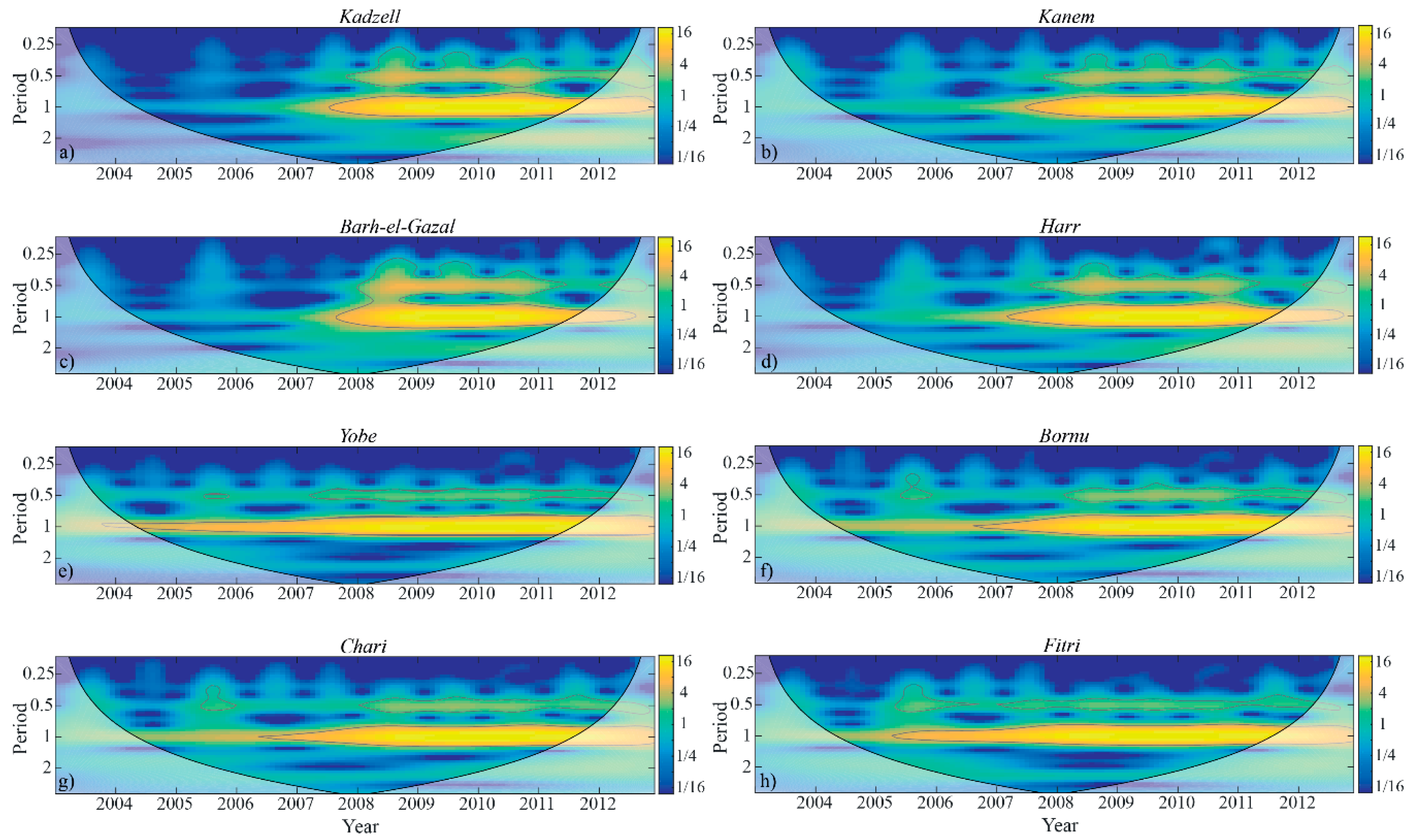
Rainfall data from Tropical Rainfall Measuring Mission (TRMM) [54]) are also used in this study. We use the monthly TRMM-merged product (3B43) [55] with a spatial resolution of 0.25°/~28 km (less accurate in time, but more accurate in space). This product shows good agreement with in situ gauge data over West Africa [56]. The period of the time series is from 1 January 2003 to 1 December 2012 and was averaged on each GRACE tiles of the Lake Chad basin [57].

Evapotranspiration, referred hereafter as ET, is obtained from the MOD16 algorithm [58] based on the algorithm of Penman-Monteith equation [59]. ET data have a spatial resolution of ~1 km and combines MODIS land cover, albedo, leaf area index (LAI), Enhanced Vegetation Index (EVI), and global surface meteorology from the Global Modeling and Assimilation Office (GMAO) meteorological data. In this study, monthly area-average ET data are used [60].

3.3. Method

The Continuous Wavelet Transform (CWT) is used to extract trends and periodicities of different time series. The Cross-Wavelet Transform (XWT) permits to analyze connection/correlation that possibly exists between two-time series. The CWT decomposes a time series into a time-frequency space, by successively convolving the time series with scaled and translated wavelet filter derived from a wavelet mother function (characterize by a zero mean) [61,62]. The Morlet wavelet is well suited for oscillations extraction, as it provides a good balance between time and frequency localization [63,64]. However, the Morlet wavelet is not precisely well located in time and thus a Cone of Influence (COI) has been introduced. Areas located inside this COI are locations on time-frequency plane where edge effects brings lower confidence in the computed values. The XWT [65,66] allows highlighting area where two time-series have a high common spectral power in time-frequency plane. The MATALB software package provided by Grinsted et al. [66] for cross-wavelet and wavelet coherence can be obtained from GitHub [67].

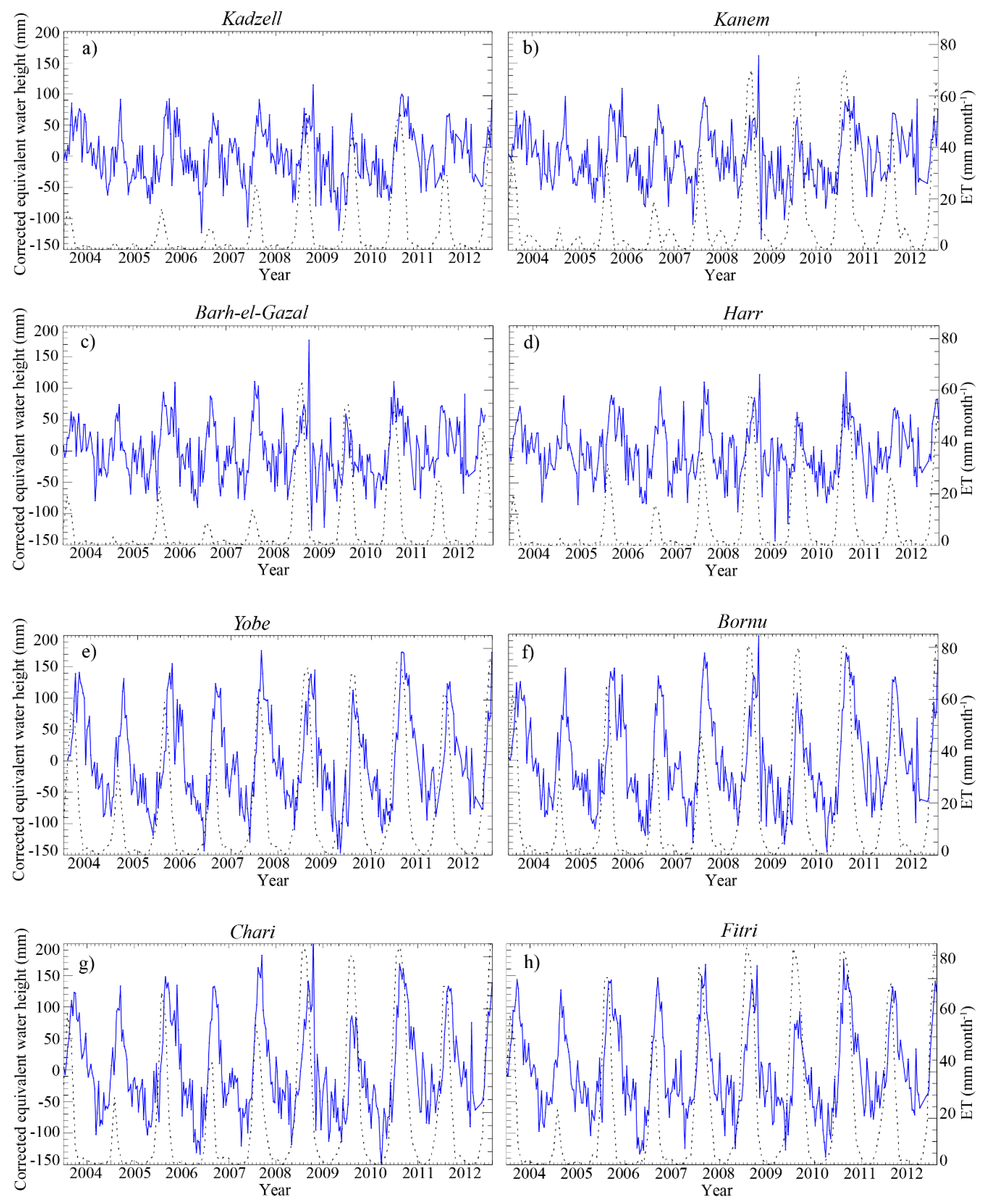
4. Temporal Evolution of the Water Mass

Figure 2 shows the evolution of the continental water storage expressed in EWH for each GRACE tiles of the region. As we are interested in understanding the different processes triggering the annual and semi-annual cycles, for each time series, a trend has been computed and removed from these GRACE solutions. The four plots in the upper panel represent the evolution of the water mass at a latitude of 14°N for the Kadzell (a), Kanem (b), Barh (c), and Harr (d) tiles. The lower part represents the water mass evolution at a latitude of 12°N for the Yobe (e), Bornu (f), Chari (g), and Fitri (h) tiles. In all plots, the most recognizable signal is the increase of water mass following WAM episodes, which ranges from −150 mm (i.e., loss of water) to 200 mm (i.e., gain of water) for the whole area. The inter-annual variability is clearly displayed and may be due to variations of the duration and intensity of the annual monsoon [68]. For each WAM episode, the response of the water mass for tiles located at the same latitude is almost the same in amplitude. The water mass variation induced by rainfalls is ~150 mm at 14°N and ~250 mm at 12°N; this latitudinal dependence is directly linked to the latitudinal shift of the ICTZ (Section 2.1) [68]. The most interesting results from these height graphs are the deceleration of water mass decrease at the beginning of the dry season or even during some years, an increase of the water mass that implies water supply in the region. This Dry Seasonal Water Increase (referred hereafter as DSWI) occurs at the beginning of the dry season and starts in average in December to last until March/April. The DSWI is more intense at 12°N (Figure 2e–h) than at 14°N (Figure 2a–d), suggesting a latitudinal dependence. Moreover, in all tiles, the DSWI signal is stronger between 2004 and 2010.

The continuous wavelet transform (CWT) analysis of the GRACE signal (Figure 3) shows that, in each tile, the maximum spectral power (referred hereafter as MSP) of the water mass signal in time frequency space is observed with a periodicity of 1 year and with less energy, at 6 months. The one year period is linked to the annual WAM episodes. The semi-annual cycle is linked to the DSWI signal of GRACE estimations. It is observable from mid-2006 to 2007 for the Kadzell, Yobe, and Bornu tiles. For the five other tiles, this semi-annual cycle is more pronounced and persists from mid-2006 to mid-2008. The CWT of GRACE estimation displays the existence of a signal at 3 months in 2005 in the Kadzell, Kanem, Harr, Yobe, and Bornu. In tiles in which the clay concentration at the surface is more important (Figure 3g,h), the 3 months period does not exceed the 5% of confidence. This observation can also be made for the Bahr-el-Gazal (Figure 3c) tile, in which the concentration of clays at the surface is low (Figure 1). As the MSP associated with the WAM phenomenon (with a periodicity of 1 year) is very strong, in order to highlight the MSP of the semi-annual cycle, the CWT of the water mass corrected from the annual cycle is presented in Figure 4. At 14°N (Figure 4a–d), the DSWI signal (with a periodicity of 6 months) is displayed from end of 2005 to 2010, except for the Kadzell tile (Figure 4a), in which the DSWI starts from mid-2004. From 2006 to 2008, the amplitude of the DSWI reaches a maximum and decreases until its disappearance in 2010. The DSWI signal in the Kadzell tile (Figure 4a) starts sooner and lasts longer than for the Kanem, Barh-el-Gazal, and Harr tiles (Figure 4b–d). At 12°N (Figure 4e–h), the DSWI cycle occurs from 2005 to 2011. As for the tiles at 14°N, the DSWI amplitude is at its maximum from 2006 to 2008 and decreases until 2011. The duration of the DSWI decreases with the longitude, as demonstrated by the comparison between the Yobe (Figure 4e) and Fitri tiles (Figure 4h). This figure also displays the existence of shorter periods of 3 and 1.5 months, as now the MSP is above the 5% confidence level. The variability of these cycles is more important after 2008. This increase of variability can be associated with climatic changes in the region.

5. Lake Chad Elevation, Rainfall, and Evapotranspiration Rate

5.1. Lake Chad Evolution

Lake Chad is at an altitude of ~282 m above sea level (a.s.l.). The recent variations in Lake Chad water elevation are obtained by altimetry [69]. These data show that after each WAM episode from 2003 to 2012, the water level variation is ~2 m from June/July until late October/early November. Then, the water level starts to decrease for 6 to 7 months before reaching the minimum water level (~279 m) in June. The wavelet transform analysis confirms the presence of the annual cycle with a period of 1 year (high wavelet coefficient, Figure 5) with a constant MSP for each WAM episode.

5.2. Rainfall Data

The WAM system drives the rainfall annual cycle and occurs from June/July to October/November over the Sahelian region. Figure 6 presents the monthly TRMM-merged rainfall data, averaged over the Kadzell (a), Kanem (b), Bahr (c), and Harr (d) tiles at 14°N, and over the Yobe (e), Bornu (f), Chari (g), and Fitri (h) tiles at 12°N. The inter-annual rainfall fluctuations are well displayed through the intensity and duration variation of the rainfall episodes. The rainfall rates reveal the strong latitudinal dependence of the WAM rainfall, as the rate decreases from ~225 mm month⁻¹ at 12°N to ~100 mm month⁻¹ at 14°N. Finally, the WAM rainfall peaks between July and September and then a sharp precipitation decrease occurs in October, as the ICTZ moves southward.

The CWT analysis of the TRMM data for each tile (Figure 7) shows the existences of a signal with a one year period and confirms the inter-annual latitudinal and local variability of the monsoon rainfall. Indeed, at 14°N (Figure 7a–d), the spectral power of the annual cycle is constant for the complete time series at Kanem (Figure 7b) and Harr (Figure 7d) tiles, while it is discontinuous for the Kadzell tile (Figure 7a) and starts only in 2005 in the Barh tile (Figure 7c). Moreover, the MSP is not reached during the same years for the different tiles. For Kanem (Figure 7b), the MSP is reached between the 2004 and the 2006-WAM episodes, while in the Barh tile (Figure 7c), the MSP lasts from the 2008-WAM episode up to the end of the time series. At 12°N (Figure 7e–h), the spectral power of the annual cycle is present for the complete time series and for all tiles. The only difference is the time length of the maximum energy. For Yobe (Figure 7e), the MSP is displayed between the 2004-WAM and 2009-WAM episodes. For the Bornu tile (Figure 7f), the spectral power linked to WAM rainfalls is less significant between mid-2009 and mid-2010. The MSP decreases between mid-2007 and mid-2009 for the Chari tile (Figure 7g) and lasts only until 2009 for the Fitri tile (Figure 7h). The comparison of the rainfall amount (Figure 6) with the associated annual period spectral power (Figure 7) suggests that the decrease of the rainfall rate induces those of the spectral power. A signal exceeding the 5% confidence level with a period of 6 and 3 months can be observed in Kadzell (Figure 7a), Barh-el-Gazal (Figure 7c), Harr (Figure 7d), Yobe (Figure 7e), and Chari (Figure 7g) tiles. In the contrary, the Kanem (Figure 7b) and Bornu (Figure 7f) tiles display only a 3 months period, while the Fitri tile (Figure 7h) is characterized by a 6 months periodic signal.

Figure 8 presents the temporal evolution of the amount of water, which is not absorbed by vegetation nor evaporated (rainfalls-ET) with 10-day GRACE data averaged by month at 14°N for the Kadzell (a), Kanem (b), Bahr (c), and Harr (d) tiles and at 12°N over the Yobe (e), Bornu (f), Chari (g), and Fitri (h) tiles. Each WAM episode is followed by an increase of the water mass after one or two months delay. For all GRACE tiles, WAM rainfalls explain between 65% and 80% of the water mass observed during the wet season. The 35% to 20% left may be explained by other processes, as river supply, that are fed more to the south (more humid zones) for the River Chari-Logone and westward for River Komadugu-Yobe. The highest water level is reached around October/November at the lake and downstream of the rivers. The rivers and Lake Chad are included only in four tiles: Kadzell (Figure 8a), Kanem (Figure 8b), Bornu (Figure 8f), and Fitri (Figure 8h). For example, Lake Chad represents ~3% of the Kanem tile surface by considering the actual average area of the inundated part of the southern basin (~1040 km²). Consequently, the water variation in the lake is ~2 m year⁻¹ and represents ~25% of the water mass evolution during the wet season. In the Bornu tile, the water level change represents ~8% of the water mass, as the inundated area only covers ~1% of the tile area.

5.3. Evapotranspiration Data

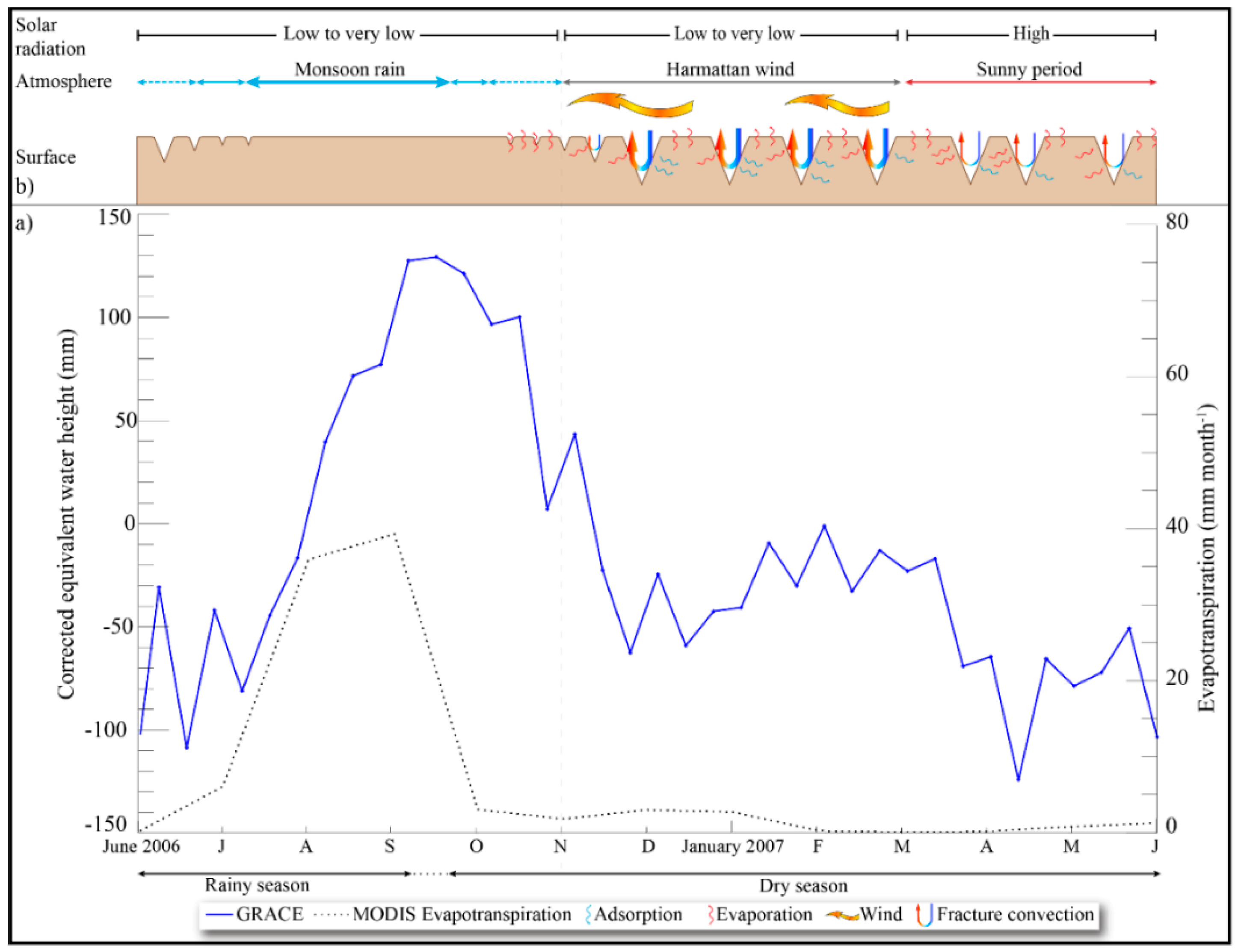
The spatial repartition of the ET rate is displayed in Figure 9. This latter map reveals that the ET rate has a latitudinal dependence. Indeed, during WAM episodes, the ET rate reaches ~1.5 m month⁻¹ at 11°N and decreases below ~100 mm month⁻¹ at 14°N. Within this general trend, ET is ~2 m month⁻¹ over the lake and permanent rivers. Now, when we study the evolution of the ET rate at the native 1-km spatial resolution, it varies with time (Figure 10). The ET rate evolution exhibits different behaviors according to the location of the pixels. The first pixel (Figure 10a) is located in the Kadzell region (dry area and a clay content at the surface of ~2%, Figure 1), the second represents the Lake Chad bed (Figure 10b), and the last one (Figure 10c) is located at 12°N, in a clay rich region (Figure 1).

The ET data of the first pixel show an ET rate of ~200 mm month⁻¹ during the rainy season up to 2008, except for the 2004-WAM episode where there is no signal. Since 2008, the ET rate has increased to ~500 mm month⁻¹. The ET rate evolution on the second pixel (Figure 10b) and the third one (Figure 10c) is particularly interesting as the signal can be divided into two periods: the first period from 2003 to early 2008 and the second one from 2008 to 2012.

The period from 2003 to 2008 presents a mean maximum with an ET rate of ~670 mm month⁻¹ in pixel (b) and ~750 mm month⁻¹ in pixel (c). In both pixels, the ET signal associated with the WAM rainfalls is recognizable. The most intriguing/surprising signal is the increase of the ET signal at the beginning of the dry season, between October/November and March/April, observed in these pixels: in pixel (b), the ET reaches in average ~400 mm month⁻¹ and ~70 mm month⁻¹ in pixel (c).

During the period from 2008 to 2012, the maximum average ET signal associated with the WAM rainfalls reaches ~920 mm month⁻¹ in pixel (b) and ~850 mm month⁻¹ in pixel (c). Then, from October/November until February/March (thus during the dry period), a slope discontinuity is visible in pixel (b) at the beginning of the dry season only in 2008 and 2012, while in pixel (c) this discontinuity is observable from 2008 to 2012.

This study of the ET rate according to different surface feature/lithology shows an interesting relationship between them. At the beginning of the dry season, the ET rate increases during 4 to 5 months before decreasing again only in the pixels where the percentage of clays at the surface is above 30% (Figure 1). As the clay amount is the only factor that varies between the three pixels, it seems that the seasonal behavior of clays along time may affects the soil moisture evolution. Now, this behavior is reported for pixels with 1-km size. The question is whether this dependence between the ET rate and the amount of clay is still reliable at GRACE resolution. Figure 10 presents the mean spatial ET rate, i.e., the averaged ET data for each GRACE tiles, with the GRACE EWH. At a latitude of 14°N (Figure 11a–d), the ET rate is ~25 mm month⁻¹ from 2003 to 2008. Since 2008, the evapotranspiration has increased to ~50 mm month⁻¹ for the Kadzell (Figure 11a), Bahr (Figure 11c), and Harr tiles (Figure 11d), and to ~60 mm month⁻¹ in the Kanem tile (Figure 11c). At a latitude of 12°N, from 2003 to 2008 and for all tiles, the ET rate is twice, in comparison with the one estimated during the same period at 14°N. From the 2008-WAM episode to the one of 2011, the ET rate reaches ~80 mm month⁻¹ (Figure 11e–h).

The CWT analysis of the MODIS ET rate data shows the spectral power evolution in time frequency space, as a function of latitude and longitude (Figure 12). At 14°N (Figure 12a–d), the spectral power of the annual cycle observed with a periodicity of 1 year is more pronounced between the WAM episodes of 2007 and 2011. The MSP is reached from the 2008-WAM episode to the one of 2010. A spectral power signal associated with a semi-annual cycle is also observed from mid-2007. There is no clear evidence of a variation with the latitude. However, the spectral power of the annual ET signal at 12°N (Figure 12e–h) shows longitudinal dependence. The annual ET spectral power periodicity of the Yobe tile (Figure 12e) is observed from the 2004-WAM episode until 2011 and the one for the Fitri tile (Figure 12h) starts in 2005. For the Bornu and Chari tiles (Figure 12f,g), the annual cycle starts in 2006. The maximum annual spectral power is reached from the 2008-WAM episodes to the 2011 one for all the four tiles. The semi-annual cycle power runs from 2007 to 2011 with a maximum associated to the WAM episodes of 2008, 2009, and 2010 at 14°N. At 12°N, semi-annual power is observed from 2005 to 2011. As for the annual cycle and the semi-annual cycle at 14°N, the maximum of spectral power is reached from the 2008 to 2010 WAM-episodes. However, during the WAM episode of 2005, the semi-annual cycle power reaches a maximum for all the four tiles.

6. Discussion

6.1. Influence of Surface Water

The most important variations of the water mass described by the GRACE solutions are due to the WAM rainfall amounts, which are indirect evidence of the significant importance of the rainfall control on the hydrology of the Lake Chad basin. The CWT analysis (Figure 7) of the rainfall data confirms the presence of the inter-annual cycle (see Section 5.2). The existence of signals with shorter periods of 6 and 3 months are not confirmed with in situ data and thus may be dependent with the data processing. Moreover, the response delay recorded in Lake Chad and its tributaries (Figure 8) is not sufficient to explain (1) the spatial correlation between the clay amount repartition with the existence of the DSWI and the ET increase at the beginning of the dry season and (2) the semi-annual cycle appearing in both DSWI and ET rate in all tiles. It appears that these years, where the water balance becomes negative (Figure 8), are periods where the ET signal does not increase at the beginning of the dry season. This observation means that at this period, we have an excess of evapotranspiration compared to the amount of available water brought by rainfalls.

6.2. Influence of Evapotranspiration

The regional ET signal is characterized by the superposition of an annual WAM system-dependent cycle and a semi-annual period that always appears between November/December and March/April. This latter semi-annual cycle, as presented in Section 3.2, is observed within pixels at the native resolution of MODIS (1 km) and at the spatial sampling of the GRACE tiles (2° × 2°). In both cases, this cycle shows a dependence with the surface lithology (Figure 10b,c, Figure 11a,g), as only pixels/tiles rich in clays (Figure 1) exhibit this semi-annual cycle. The cross-wavelet coherence between MODIS ET and GRACE data (Figure 13) shows good cross-correlation between both signals for the 1 year and 6 months periods. In more details, at 14°N (Figure 13a–d), the annual and 6 months periods cross-correlation start around 2007 for the four tiles. At 12°N (Figure 13e–h), the annual period cross-correlation is observed for the entire series, while the one for the 6 months period starts around 2006. Figure 14a shows that a delay of one or two months exists between the DSWI and the ET increase during the wet season and at the beginning of the dry season. These results are confirmed by the observed phase delay between ET and DWSI close to the 45° of the XWT (ET event occurs before the DWSI). Consequently, we suppose that the process behind the ET increase is the same as the one responsible for the DSWI.

As stated by [66], it is quite difficult to go further in the interpretation of the cross wavelet transform, as the mechanism that explains the evolution of the ET and the water mass remains unknown. However, the most important result to keep in mind is the good relationship observed between the presence of clays at the surface with the existence of the ET rate increase and the DSWI signal. This can be explained by the relatively high water adsorption capacity of clays, which induces an evaporative surface close to the soil-atmosphere interface, and thus a higher evaporation flux. The spatial variation of the surface vertical permeability has a non-negligible impact in the seasonal and diurnal water vapor cycle [12]. In order to understand how this surface vertical permeability has such an influence on the ET rate and the DSWI, we suppose that seasonal variation of the water content in clay is the main controlling factor (Figure 14a,b).

6.3. Influence of the Surface Permeability of Clays

Clay-rich deposits, in continental conditions, are characterized by the development of desiccation cracks that form during layer contraction and dewatering [70,71,72]. Width of desiccation cracks ranges from a few centimeters from experiment in slurry [73,74,75,76] to ~30 cm in natural clay deposits [71,77] with rich content in smectite. In the Lake Chad basin, the presence of desiccation cracks has been reported in different areas. In the Kanem region, although its surface is mainly constituted by aeolian sand, desiccation cracks develop in clay deposited in depressions between dunes. The size of these cracks can reach 30 cm deep and 10 cm wide [32,78], and the mean radius of these clay polygons ranges from 5 to 10 cm [79]. Desiccation cracks have also been reported in the flood plain of the River Chari-Logone [35,80] and in the Lake Chad bed, where their size can reach several centimeters in width and one meter in depth [81]. All these desiccation cracks begin to form at the end of the rainy season (Figure 14b). During the Harmattan period, they may grow more quickly under the effect of the wind and are progressively filled by sand [78,81]. These soil cracks increase the vertical permeability of clay-rich deposits (mean permeability ≤ 10⁻¹⁶ m²) and are pathways for fluids, especially in arid and semi-arid contexts (e.g., [82]). Indeed, these cracks have been studied for their role in aquifer recharge under humid conditions and are considered as inactive during dry seasons [83,84]. However, desiccation cracks permit gas flux across unsaturated zones and the atmosphere by (i) wind pumping, (ii) atmospheric barometric changes, and (iii) thermally-driven convection flow in fractures during dry seasons [83,84,85]. The first two processes result in the advection of underground air towards the atmosphere [85], but are infrequent, as they depend on meteorological conditions. Thermally-driven convection flow inside cracks/fractures happens daily, only during winter nights in middle-latitudes, when the air inside cracks/fractures is warmer and less dense than the atmospheric air. During sunset, as the atmosphere cools down, unstable air-density gradient develops, creating an air overturning within the cracks/fractures [83,84,85]. This thermally-driven free convection is a venting of warm moist air from the cracks/fractures replaced by a cool, relatively dry air and thus enhances the evaporation from within cracks/fractures [83,84]. Indeed, Nachshon et al. [85] (and references therein) estimated that nightly evaporation process, controlled by thermal convection, is of similar order of magnitude, as the one occurring at day.

Moisture contribution in semi-arid to arid areas is regularly provided by dew and/or adsorption and in some cases only by adsorption [86,87,88]. Moisture contribution is controlled by the surface temperature (dew happens only when the surface temperature drops below the dew point), while adsorption in the soil is controlled by the relative humidity that starts only when the soil relative humidity is lower than that of the atmosphere. Agam and Berliner [87] have shown that in most semi-arid to arid areas, moisture contribution is essentially controlled by vapor adsorption during the dry season. On the Lake Chad basin, in situ data at the N’Djamena station (12.13°N, 15.03°E) from African Monsoon Multidisciplinary Analysis (AMMA) [89,90] shows that during the dry season, the dew point temperature is mostly negative. According to [87], and considering the in situ evaluation of the dew temperature, we suppose that the main process of the moisture contribution is linked to vapor adsorption. AMMA samples of the diurnal evolution of atmospheric relative humidity show that the relative humidity at night ranges from ~62% in October to ~35% in December (when an increase of the ET and GRACE signal is observed) (Figure 14a); thus, we will consider a mean relative humidity for October to December of ~45%.

From November to March, the Harmattan wind blows and creates a subsequent drop of the nighttime temperature (see Section 2.1), possibly leading to the occurrence of thermally-driven air convection in fractures. As the soil has started to be dehydrated, we can reasonably suppose that the atmospheric relative humidity at night is greater than the one inside the soil. In that case, at this time of the year, as the atmospheric relative humidity is still significant, air convection allows water vapor inside the surface through the desiccation cracks (Figure 14b) and hydration of smectite by adsorption can occur. Taking an average value of d = 3 × 10⁻¹⁰ m² s⁻¹ for the water diffusion coefficient inside clays (montmorillonite or kaolinite) [91,92] and a radius d of 5 cm for the polygon, the diffusion time through clay polygons is

$$\frac{d^2}{\kappa }=4\times {10}^{6}s$$

(1)

Thus, the diffusion time is, on average, 96 days. Interestingly, the DSWI signal in the GRACE tiles lasts for 3 months. The variation of the water mass at this period ranges from few tens of millimeters to, exceptionally, 100 millimeters. For most of the years, the increase does not exceed 70 mm. Knowing that for an atmospheric relative humidity of ~45%, a clay constituted by montmorillonite can adsorb 0.12 g of water per gram of clay [93], we estimate that this leads to the addition of ~8 cm of water per m² of clays. This estimation is correct if the clays are mainly constituted by montmorillonite. Indeed, Hatch et al. [93] have demonstrated that the adsorption process can only bring 0.035 g of water per gram of kaolinite. Thus, this value of 8 cm of water per m² of clays represents the maximum potentiality of the adsorption process to explain (1) the DSWI observed at the beginning of the dry season and (2) why the ET increase as a part of this water, adsorbed at night, is available the following day (Figure 14a).

Convective venting from fractures is a phenomenon only described for its influence on the soil-atmosphere gas exchanges and particularly on water vapor flux [85]. Evaporation via convective venting is the most studied one. It reveals that the impact of evaporation from fractures and/or faults at the basin scale is important enough to be evaluated in the context of the regional water mass variation. It has been proposed for arid environments that venting of moist fracture air can significantly enhance signal of evaporative water losses [83]. In the case of Lake Chad basin, our results suggest that under specific conditions, air convection inside desiccation cracks can increase the quantity of water inside polygons through the process of adsorption [87]. This process of adsorption is stronger when montmorillonites are present, because their particles have the largest capacity of adsorption due to a high specific surface area varying from 300 to 800 m² g⁻¹ [94,95]. For comparison, the quantity of water adsorbed in quartz sand for the same relative humidity considered in Equation (1) is ~0.2 mg of water per gram of sand [89]. This behavior results from the low specific surface area of quartz sand that is 0.34 m² g⁻¹ [96]. Moreover, Morris et al. [97] have figured out that the water loss is more significant from the sides of the cracks, because the soil there is wetter than the soil at the ground surface. This result explains the amplitudes observed in this study between clay contents, the existence of the ET increase and the DSWI signal, and their relationship with the occurrence of desiccation cracks during the Harmattan period (Figure 14a,b).

The difference in behavior of the ET rate and water mass evolution prior and after 2008 is quite striking. The TRMM data show a slight increase of the WAM rainfalls for the 2008 and 2010 episodes. However, the ET rate behaves differently prior to and after 2008 (Section 5.3). The increase of the ET and DSWI signals at the beginning of the dry season is clearly present before 2008. Studies have demonstrated the importance of dependence in multi-year cycles of antecedent soil moisture on the crack density [98]. As there is a direct link between rainfalls and soil moisture changes, it is possible that the amount of previous rainfalls and/or rainfall anomalies occurring at the end of the season [7] controls the cracks density and the quantity of adsorbed water into a system of desiccated cracks.

Such a study highlights the sub-annual relationship between the nature of the soil (considered as an interface of exchange) and the geographical water storage variability seen by space gravimetry, when distinguishing sandy and clay-rich environments. This spatialization implies different conditions of water availability (forced by low atmosphere conditions at the surface), and that also have an impact on the draining process down to groundwater. In particular, these GRACE-based time scales of available surface soil water would provide useful constraints in regional modelling of groundwater replenishment by percolation.

7. Conclusions

In this study, multi-year GRACE measurements of water storage changes in the Lake Chad basin demonstrate the ability of GRACE data to retrieve the annual water mass variation due to the WAM phenomenon. GRACE measurements also display the existence of an increase of the water storage (DSWI) at the beginning of the dry season. The DSWI occurs from December to March/April when there is no water made available through rainfalls and when the rivers/lakes water level variations are only associated with the WAM system. However, MODIS ET data display an increase of the ET rate during the rainfall period but also at the beginning of the dry season, one or two months before the DSWI signal on GRACE data. The possible existence of a relationship between the DSWI and the ET data is confirmed by the cross-wavelet coherence between both signals. The ET rate shows a strong relationship with the clay amount at the surface. Thus, in order to explain the link between the ET increase and the DSWI of the water storage, and to understand the origin of the DSWI while considering the influence of soil variations of clay amounts at the surface, we propose that soil conditions influence the exchanges at the soil-atmosphere interface, more precisely the water content (i.e., soil suction). We show that clay-rich pixels/tiles show a stronger ET and DSWI increase than for sandy soils. Due to their highly specific surface area that can reach more than 500 m² g⁻¹, montmorillonites have a larger water adsorption than quartz sand, which has a very low specific surface area of 0.34 m² g⁻¹. Moreover, the presence of desiccation cracks increases the surface of exchanges between the subsurface and the atmosphere; at macroscopic scale by wind pumping, barometric changes, and thermal convection through the fractures; and at microscopic scale, by variation of the soil suction inside the fractures. Although the first two processes are dependent upon the meteorological conditions, convective venting in the cracks/fractures of the soil occurs daily under specific conditions. The most important one is the temperature difference between the atmosphere and the one contained in the fractures. We assume that during the Harmattan (dust load wind that leads to a subsequent drop of nighttime temperature) period, at night, the atmospheric temperature is colder than the air inside the fractures, thus leading to a thermally-driven convection inside those fractures. As moisture contribution in arid to semi-arid areas is controlled by water adsorption, we propose that air convection inside the desiccation cracks brings enough water to the system to increase the total water content in the unsaturated zone. A part of the adsorbed water is available for evapotranspiration the following day, thus increasing the ET rate during the Harmattan period.

During this study, we propose a scenario that permits to link processes occurring at large temporal and spatial scales, provided with space-based data and the ones occurring at much smaller spatio-temporal scales. This study brings new elements of response to the semi-annual dynamics of the water mass variations: it shows the importance of small temporal scale of the evapotranspiration rate in the modeling of soil moisture in this region controlled by the seasonal variation of the vertical permeability in clay-rich soils.

References

1. Grodsky, S.A.; Carton, J.A. Coupled land/atmosphere interactions in the West African Monsoon. Geophys. Res. Lett. 2001, 28, 1503–1506. [Google Scholar] [CrossRef] [Green Version]
2. Sultan, B.; Janicot, S. Abrupt shift of the ITCZ over West Africa and intra-seasonal variability. Geophys. Res. Lett. 2000, 27, 3353–3356. [Google Scholar] [CrossRef] [Green Version]
3. Sultan, B.; Janicot, S. The West African Monsoon Dynamics. Part II: The “Preonset” and “Onset” of the Summer Monsoon. J. Clim. 2003, 16, 3407–3427. [Google Scholar] [CrossRef]
4. Louvet, S.; Janicot, S. Study of the first guinean rainy season and role of the subtropical jet of the northern hemisphere. In Proceedings of the EGS-AGU-EUG Joint Assembly, Nice, France, 6–11 April 2003; p. 9321. [Google Scholar]
5. Sultan, B.; Janicot, S.; Diedhiou, A. The West African Monsoon Dynamics. Part I: Documentation of Intraseasonal Variability. J. Clim. 2003, 16, 3389–3406. [Google Scholar] [CrossRef]
6. Matthews, A.J. Intraseasonal Variability over Tropical Africa during Northern Summer. J. Clim. 2004, 17, 2427–2440. [Google Scholar] [CrossRef] [Green Version]
7. Fontaine, B.; Louvet, S.; Roucou, P. Fluctuations in annual cycles and inter-seasonal memory in West Africa: Rainfall, soil moisture and heat fluxes. Theor. Appl. Climatol. 2007, 88, 57–70. [Google Scholar] [CrossRef]
8. Koster, R.D.; Dirmeyer, P.A.; Guo, Z.; Bonan, G.; Chan, E.; Cox, P.; Gordon, C.T.; Kanae, S.; Kowalczyk, E.; Lawrence, D.; et al. Regions of Strong Coupling Between Soil Moisture and Precipitation. Science 2004, 305, 1138–1140. [Google Scholar] [CrossRef] [PubMed]
9. Leblanc, M.; Razack, M.; Dagorne, D.; Mofor, L.; Jones, C. Application of METEOSAT thermal data to map soil infiltrability in the central part of the Lake Chad basin, Africa. Geophys. Res. Lett. 2003, 30. [Google Scholar] [CrossRef]
10. Schneider, J.L.; Wolff, J.P. Carte Géologique et Hydrogéologique à 1/1,500,000 de la république du Tchad. Mémoire explicatif; BRGM: Orleans, France, 1992; Volume 2, p. 571. [Google Scholar]
11. Aranyossy, J.F.; Ndiaye, B. Étude et modélisation de la formation des dépressions piézométriques en Afrique sahelienne. J. Water Sci. 1993, 6, 81–96. [Google Scholar] [CrossRef]
12. Lopez, T.; Antoine, R.; Kerr, Y.; Darrozes, J.; Rabinowicz, M.; Ramillien, G.; Cazenave, A.; Genthon, P. Subsurface Hydrology of the Lake Chad Basin from Convection Modelling and Observations. Surv. Geophys. 2016, 37, 471–502. [Google Scholar] [CrossRef]
13. Save, H.; Bettadpur, S.; Tapley, B.D. High-resolution CSR GRACE RL05 mascons. J. Geophys. Res. Solid Earth 2016, 121, 7547–7569. [Google Scholar] [CrossRef]
14. Tapley, B.D.; Bettadpur, S.; Ries, J.C.; Thompson, P.F.; Watkins, M.M. GRACE Measurements of Mass Variability in the Earth System. Science 2004, 305, 503–505. [Google Scholar] [CrossRef] [PubMed] [Green Version]
15. Grippa, M.; Kergoat, L.; Frappart, F.; Araud, Q.; Boone, A.; de Rosnay, P.; Lemoine, J.-M.; Gascoin, S.; Balsamo, G.; Ottlé, C.; et al. Land water storage variability over West Africa estimated by Gravity Recovery and Climate Experiment (GRACE) and land surface models. Water Resour. Res. 2011, 47, W05549. [Google Scholar] [CrossRef]
16. Nahmani, S.; Bock, O.; Bouin, M.-N.; Santamaŕıa-Gómez, A.; Boy, J.-P.; Collilieux, X.; Métivier, L.; Panet, I.; Genthon, P.; de Linage, C.; et al. Hydrological deformation induced by the West African Monsoon: Comparison of GPS, GRACE and loading models. J. Geophys. Res. Solid Earth 2012, 117. [Google Scholar] [CrossRef] [Green Version]
17. Swenson, S.; Famiglietti, J.; Basara, J.; Wahr, J. Estimating profile soil moisture and groundwater variations using GRACE and Oklahoma Mesonet soil moisture data. Water Resour. Res. 2008, 44, W01413. [Google Scholar] [CrossRef]
18. Pfeffer, J.; Champollion, C.; Favreau, G.; Cappelaere, B.; Hinderer, J.; Boucher, M.; Nazoumou, Y.; Oï, M.; Mouyen, M.; Henri, C.; et al. Evaluating surface and subsurface water storage variations at small time and space scales from relative gravity measurements in semiarid Niger. Water Resour. Res. 2013, 49, 3276–3291. [Google Scholar] [CrossRef]
19. Ramillien, G.; Frappart, F.; Seoane, L. Application of the regional water mass variations from GRACE satellite gravimetry to large-scale water management in Africa. Remote Sens. 2014, 6, 7379–7405. [Google Scholar] [CrossRef]
20. Bader, J.-C.; Lemoalle, J.; Leblanc, M. Modèle hydrologique du Lac Tchad. Hydrol. Sci. J. 2011, 56, 411–425. [Google Scholar] [CrossRef] [Green Version]
21. Descloitres, M.; Chalikakis, K.; Legchenko, A.; Moussa, A.M.; Genthon, P.; Favreau, G.; Coz, M.L.; Boucher, M.; Oï, M. Investigation of groundwater resources in the Komadugu Yobe Valley (Lake Chad Basin, Niger) using MRS and TDEM methods. J. Afr. Earth Sci. 2013, 87, 71–85. [Google Scholar] [CrossRef]
22. Adedokun, J.A.; Emofurieta, W.O.; Adedeji, O.A. Physical, mineralogical and chemical properties of harmattan dust at Ile-Ife, Nigeria. Theor. Appl. Clim. 1989, 40, 161–169. [Google Scholar] [CrossRef]
23. Schuster, M.; Roquin, C.; Duringer, P.; Brunet, M.; Caugy, M.; Fontugne, M.; Mackaye, H.T.; Vignaud, P.; Ghienne, J.-F. Holocene Lake Mega-Chad palaeoshorelines from space. Quat. Sci. Rev. 2005, 24, 1821–1827. [Google Scholar] [CrossRef]
24. Leblanc, M.; Favreau, G.; Maley, J.; Nazoumou, Y.; Leduc, C.; Stagnitti, F.; van Oevelen, P.J.; Delclaux, F.; Lemoalle, J. Reconstruction of Megalake Chad using Shuttle Radar Topographic Mission data. Palaeogeogr. Palaeoclim. Palaeoecol. 2006, 239, 16–27. [Google Scholar] [CrossRef]
25. Crétaux, J.-F.; Birkett, C. Lake studies from satellite radar altimetry. C. R. Geosci. 2006, 338, 1098–1112. [Google Scholar] [CrossRef]
26. Coe, M.T.; Birkett, C.M. Calculation of river discharge and prediction of lake height from satellite radar altimetry: Example for the Lake Chad basin. Water Resour. Res. 2004, 40, W10205. [Google Scholar] [CrossRef]
27. Seeber, K. 2nd Misson on Discharge Measurements at Chari, Logone and Koulambou River, Chad; Lake Chad Basin Commission, 2013; Available online: http://www.cblt.org/sites/default/files/download_documents/bgr_report_6_engl.pdf (accessed on 4 June 2018).
28. Leduc, C.; Salifou, O.; Leblanc, M. Evolution des ressources en eau dans le département de Diffa (bassin du lac Tchad, sud-est nigérien). In Water Resources Variability in Africa during the XXth Century; IAHS Publications: Oxfordshire, UK, 1998; Volume 252. [Google Scholar]
29. Genik, G.J. Regional framework, structural and petroleum aspects of rift basins in Niger, Chad and the Central African Republic (C.A.R.). Tectonophysics 1992, 213, 169–185. [Google Scholar] [CrossRef]
30. Olugbemiro, O.R.; Ligouis, B. Thermal maturity and hydrocarbon potential of the Cretaceous (Cenomanian-Santonian) sediments in the Bornu (Chad) basin, NE Nigeria. Bull. Soc. Geol. Fr. 1999, 170, 759–772. [Google Scholar]
31. Griffin, D.L. The late Neogene Sahabi rivers of the Sahara and their climatic and environmental implications for the Chad Basin. J. Geol. Soc. 2006, 163, 905–921. [Google Scholar] [CrossRef]
32. Servant, M. Données stratigraphiques sur le Quaternaire supérieur et récent au nord-est du Lac Tchad. Cah. ORSTOM 1970, 2, 95–114. [Google Scholar]
33. Edmunds, W.M.; Fellman, E.; Goni, I.B. Lakes, groundwater and palaeohydrology in the Sahel of NE Nigeria: Evidence from hydrogeochemistry. J. Geol. Soc. 1999, 156, 345–355. [Google Scholar] [CrossRef]
34. Schuster, M.; Duringer, P.; Ghienne, J.-F.; Roquin, C.; Sepulchre, P.; Moussa, A.; Lebatard, A.-E.; Mackaye, H.T.; Likius, A.; Vignaud, P.; et al. Chad Basin: Paleoenvironments of the Sahara since the Late Miocene. C. R. Geosci. 2009, 341, 603–611. [Google Scholar] [CrossRef]
35. Schneider, J.L.; Wolff, J.P. Carte Géologique et Hydrogéologique à 1/1,500,000 de la république du Tchad. Mémoire explicatif; BRGM: Orleans, France, 1992; Volume 1, p. 435. [Google Scholar]
36. Durand, A.; Mathieu, P. Evolution paléogéographique et paléoclimatique du bassin tchadien au Pléistocène supérieur. Rev. Geol. Dyn. Geogr. Phys. 1980, 22, 329–341. [Google Scholar]
37. Jesus, T.H. Jorge Samuel Mendes de SoilGrids|ISRIC. Available online: http://soilgrids.org (accessed on 3 February 2017).
38. Hofmann-Wellenhof, B.; Moritz, H. Physical Geodesy; Springer Science & Business Media: Berlin, Germany, 2006. [Google Scholar]
39. Bettadpur, S. Level-2 Gravity Field Product User Handbook; The GRACE Project; Jet Propulsion Laboratory: Pasadena, CA, USA, 2007. [Google Scholar]
40. Flechtner, F. AOD1B Product Description Document for Product Releases 01 to 04 (Rev. 3.1, April 13 2007). GRACE Project Document; 2007; pp. 327–750. Available online: http://op.gfz-potsdam.de/grace/results/grav/AOD1B_PDD_20070413.pdf (accessed on 4 June 2018).
41. Chambers, D.P.; Bonin, J.A. Evaluation of Release-05 GRACE time-variable gravity coefficients over the ocean. Ocean Sci. 2012, 8, 859. [Google Scholar] [CrossRef]
42. Dahle, C.; Flechtner, F.; Gruber, C. GFZ GRACE Level-2 Processing Standards Document for Level-2 Product Release 0005; GeoForschungsZentrum Potsdam: Potsdam, Germany, 2012. [Google Scholar]
43. Han, S.-C.; Jekeli, C.; Shum, C. Time-variable aliasing effects of ocean tides, atmosphere, and continental water mass on monthly mean GRACE gravity field. J. Geophys. Res. Solid Earth 2004, 109. [Google Scholar] [CrossRef] [Green Version]
44. Thompson, P.F.; Bettadpur, S.V.; Tapley, B.D. Impact of short period, non-tidal, temporal mass variability on GRACE gravity estimates. Geophys. Res. Lett. 2004, 31. [Google Scholar] [CrossRef] [Green Version]
45. Ray, R.D.; Luthcke, S.B. Tide model errors and GRACE gravimetry: Towards a more realistic assessment. Geophys. J. Int. 2006, 167, 1055–1059. [Google Scholar] [CrossRef]
46. Forootan, E.; Didova, O.; Schumacher, M.; Kusche, J.; Elsaka, B. Comparisons of atmospheric mass variations derived from ECMWF reanalysis and operational fields, over 2003–2011. J. Geod. 2014, 88, 503–514. [Google Scholar] [CrossRef] [Green Version]
47. Seo, K.-W.; Wilson, C.R.; Chen, J.; Waliser, D.E. GRACE’s spatial aliasing error. Geophys. J. Int. 2008, 172, 41–48. [Google Scholar] [CrossRef]
48. Swenson, S.; Wahr, J. Post-processing removal of correlated errors in GRACE data. Geophys. Res. Lett. 2006, 33. [Google Scholar] [CrossRef] [Green Version]
49. Ramillien, G.; Biancale, R.; Gratton, S.; Vasseur, X.; Bourgogne, S. GRACE-derived surface water mass anomalies by energy integral approach: Application to continental hydrology. J. Geod. 2011, 85, 313–328. [Google Scholar] [CrossRef]
50. Ramillien, G.L.; Seoane, L.; Frappart, F.; Biancale, R.; Gratton, S.; Vasseur, X.; Bourgogne, S. Constrained Regional Recovery of Continental Water Mass Time-variations from GRACE-based Geopotential Anomalies over South America. Surv. Geophys. 2012, 33, 887–905. [Google Scholar] [CrossRef] [Green Version]
51. Frappart, F.; Seoane, L.; Ramillien, G. Validation of GRACE-derived terrestrial water storage from a regional approach over South America. Remote Sens. Environ. 2013, 137, 69–83. [Google Scholar] [CrossRef] [Green Version]
52. Seoane, L.; Ramillien, G.; Frappart, F.; Leblanc, M. Regional GRACE-based estimates of water mass variations over Australia: Validation and interpretation. Hydrol. Earth Syst. Sci. 2013, 17, 4925–4939. [Google Scholar] [CrossRef]
53. TeodolinaLopez 10-Days-GRACE. Available online: https://github.com/TeodolinaLopez/10-days-GRACE (accessed on 21 March 2018).
54. Kummerow, C.; Simpson, J.; Thiele, O.; Barnes, W.; Chang, A.T.C.; Stocker, E.; Adler, R.F.; Hou, A.; Kakar, R.; Wentz, F.; et al. The Status of the Tropical Rainfall Measuring Mission (TRMM) after Two Years in Orbit. J. Appl. Meteorol. 2000, 39, 1965–1982. [Google Scholar] [CrossRef] [Green Version]
55. Adler, R.F.; Huffman, G.J.; Bolvin, D.T.; Curtis, S.; Nelkin, E.J. Tropical Rainfall Distributions Determined Using TRMM Combined with Other Satellite and Rain Gauge Information. J. Appl. Meteorol. 2000, 39, 2007–2023. [Google Scholar] [CrossRef] [Green Version]
56. Nicholson, S.E.; Some, B.; McCollum, J.; Nelkin, E.; Klotter, D.; Berte, Y.; Diallo, B.M.; Gaye, I.; Kpabeba, G.; Ndiaye, O.; et al. Validation of TRMM and Other Rainfall Estimates with a High-Density Gauge Dataset for West Africa. Part II: Validation of TRMM Rainfall Products. J. Appl. Meteorol. 2003, 42, 1355–1368. [Google Scholar] [CrossRef]
57. GES DISC. Available online: https://disc.gsfc.nasa.gov/ (accessed on 28 August 2017).
58. Mu, Q.; Zhao, M.; Running, S.W. Improvements to a MODIS global terrestrial evapotranspiration algorithm. Remote Sens. Environ. 2011, 1781–1800. [Google Scholar] [CrossRef]
59. Monteith, J.L. Evaporation and environment. Symp. Soc. Exp. Biol. 1965, 19, 205–223. [Google Scholar] [PubMed]
60. MOD16. Available online: http://files.ntsg.umt.edu/data/NTSG_Products/MOD16/ (accessed on 20 January 2017).
61. Meyer, Y.; Roques, S. (Eds.) Progress in Wavelet Analysis and Applications: Proceedings of the International Conference “Wavelets and Applications”, Toulouse, France, June 1992; Editions Frontieres: Paris, France, 1993; ISBN 2-86332-130-7. [Google Scholar]
62. Gaillot, P.; Darrozes, J.; Bouchez, J.-L. Wavelet transform: A future of rock fabric analysis? J. Struct. Geol. 1999, 21, 1615–1621. [Google Scholar] [CrossRef]
63. Morlet, J.; Arens, G.; Fourgeau, E.; Glard, D. Wave propagation and sampling theory—Part I: Complex signal and scattering in multilayered media. Geophyscis 1982, 47, 203–221. [Google Scholar] [CrossRef]
64. Goupillaud, P.; Grossmann, A.; Morlet, J. Cycle-octave and related transforms in seismic signal analysis. Geoexploration 1984, 23, 85–102. [Google Scholar] [CrossRef]
65. Prokoph, A.; Bilali, H.E. Cross-Wavelet Analysis: A Tool for Detection of Relationships between Paleoclimate Proxy Records. Math. Geosci. 2008, 40, 575–586. [Google Scholar] [CrossRef]
66. Grinsted, A.; Moore, J.C.; Jevrejeva, S. Application of the cross wavelet transform and wavelet coherence to geophysical time series. Nonlinear Process. Geophys. 2004, 11, 561–566. [Google Scholar] [CrossRef] [Green Version]
67. Grinsted, A. A Cross Wavelet and Wavelet Coherence Toolbox for MATLAB. Available online: https://github.com/grinsted/wavelet-coherence (accessed on 20 January 2017).
68. Le Barbé, L.; Lebel, T.; Tapsoba, D. Rainfall Variability in West Africa during the Years 1950–1990. J. Clim. 2002, 15, 187–202. [Google Scholar] [CrossRef]
69. Hydroweb. Available online: http://hydroweb.theia-land.fr/ (accessed on 5 July 2017).
70. Baer, J.U.; Kent, T.F.; Anderson, S.H. Image analysis and fractal geometry to characterize soil desiccation cracks. Geoderma 2009, 154, 153–163. [Google Scholar] [CrossRef]
71. Li, J.H.; Zhang, L.M. Study of desiccation crack initiation and development at ground surface. Eng. Geol. 2011, 123, 347–358. [Google Scholar] [CrossRef]
72. Lopez, T.; Antoine, R.; Darrozes, J.; Rabinowicz, M.; Baratoux, D. Development and evolution of the size of polygonal fracture systems during fluid-solid separation in clay-rich deposits. J. Earth Sci. 2018, 1–16. [Google Scholar] [CrossRef]
73. Rayhani, M.H.; Yanful, E.K.; Fakher, A. Desiccation-induced cracking and its effect on the hydraulic conductivity of clayey soils from Iran. Can. Geotech. J. 2007, 44, 276–283. [Google Scholar] [CrossRef]
74. Rayhani, M.H.T.; Yanful, E.K.; Fakher, A. Physical modeling of desiccation cracking in plastic soils. Eng. Geol. 2008, 97, 25–31. [Google Scholar] [CrossRef]
75. Tang, C.-S.; Cui, Y.-J.; Tang, A.-M.; Shi, B. Experiment evidence on the temperature dependence of desiccation cracking behavior of clayey soils. Eng. Geol. 2010, 114, 261–266. [Google Scholar] [CrossRef] [Green Version]
76. Tang, C.-S.; Shi, B.; Liu, C.; Suo, W.-B.; Gao, L. Experimental characterization of shrinkage and desiccation cracking in thin clay layer. Appl. Clay Sci. 2011, 52, 69–77. [Google Scholar] [CrossRef]
77. Weinberger, R. Initiation and growth of cracks during desiccation of stratified muddy sediments. J. Struct. Geol. 1999, 21, 379–386. [Google Scholar] [CrossRef]
78. Maglione, G. Géochimie des Évaporites et Silicates Néoformés en Milieu Continental Confiné: Les Dépressions Interdunaires du Tchad-Afrique; Travaux et Documents de l’ORSTOM; ORSTOM: Paris, France, 1976; ISBN 978-2-7099-0404-9. [Google Scholar]
79. Cheverry, C. Les Premières Étapes de la Poldérisation sur les Bordures nord-est du lac Tchad: Aspects Hydrologiques, Pédologiques, Agronomiques: Conséquences sur la Mise en Valeur; ORSTOM: Paris, France, 1971. [Google Scholar]
80. Roche, M.-A. Traçage Naturel Salin et Isotopique des eaux du Système Hydrologique du lac Tchad; ORSTOM: Paris, France, 1980. [Google Scholar]
81. Dupont, B. Etude Sédimentologique du Lac Tchad: Premiers Résultats. Office de la Recherche Scientifique et Technique Outre-mer: France, 1967; Available online: http://horizon.documentation.ird.fr/exl-doc/pleins_textes/divers14-04/12414.pdf (accessed on 4 June 2018).
82. Baram, S.; Kurtzman, D.; Dahan, O. Water percolation through a clayey vadose zone. J. Hydrol. 2012, 424–425, 165–171. [Google Scholar] [CrossRef]
83. Weisbrod, N.; Dragila, M.I. Potential impact of convective fracture venting on salt-crust buildup and ground-water salinization in arid environments. J. Arid Environ. 2006, 65, 386–399. [Google Scholar] [CrossRef]
84. Weisbrod, N.; Dragila, M.I.; Nachshon, U.; Pillersdorf, M. Falling through the cracks: The role of fractures in Earth-atmosphere gas exchange. Geophys. Res. Lett. 2009, 36, L02401. [Google Scholar] [CrossRef]
85. Nachshon, U.; Weisbrod, N.; Dragila, M.I.; Ganot, Y. The Importance of Advective Fluxes to Gas Transport Across the Earth-Atmosphere Interface: The Role of Thermal Convection. In Planet Earth 2011-Global Warming Challenges and Opportunities for Policy and Practice; Carayannis, E., Ed.; InTech, 2011; Available online: https://www.intechopen.com/books/planet-earth-2011-global-warming-challenges-and-opportunities-for-policy-and-practice/the-importance-of-advective-fluxes-to-gas-transport-across-the-earth-atmosphere-interface-the-role-o (accessed on 4 June 2018).[Green Version]
86. Agam, N.; Berliner, P.R. Diurnal Water Content Changes in the Bare Soil of a Coastal Desert. J. Hydrometeorol. 2004, 5, 922–933. [Google Scholar] [CrossRef] [Green Version]
87. Agam, N.; Berliner, P.R. Dew formation and water vapor adsorption in semi-arid environments—A review. J. Arid Environ. 2006, 65, 572–590. [Google Scholar] [CrossRef]
88. Katata, G.; Nagai, H.; Ueda, H.; Agam, N.; Berliner, P.R. Development of a Land Surface Model Including Evaporation and Adsorption Processes in the Soil for the Land–Air Exchange in Arid Regions. J. Hydrometeorol. 2007, 8, 1307–1324. [Google Scholar] [CrossRef]
89. Lebel, T.; Cappelaere, B.; Galle, S.; Hanan, N.; Kergoat, L.; Levis, S.; Vieux, B.; Descroix, L.; Gosset, M.; Mougin, E.; et al. AMMA-CATCH studies in the Sahelian region of West-Africa: An overview. J. Hydrol. 2009, 375, 3–13. [Google Scholar] [CrossRef] [Green Version]
90. AMMA—The AMMA Database. Available online: http://amma-international.org/data/ (accessed on 4 June 2018).
91. Chemkhi, S.; Zagrouba, F. Water diffusion coefficient in clay material from drying data. Desalination 2005, 185, 491–498. [Google Scholar] [CrossRef]
92. Sanchez Gonzalez, F. Water Diffusion through Compacted Clays Analyzed by Neutron Scattering and Tracer Experiments. Ph.D. Thesis, University of Bern, Bern, Switzerland, 2007. [Google Scholar]
93. Hatch, C.D.; Wiese, J.S.; Crane, C.C.; Harris, K.J.; Kloss, H.G.; Baltrusaitis, J. Water Adsorption on Clay Minerals As a Function of Relative Humidity: Application of BET and Freundlich Adsorption Models. Langmuir 2012, 28, 1790–1803. [Google Scholar] [CrossRef] [PubMed]
94. Yuang, P.-C.; Shen, Y.-H. Determination of the surface area of smectite in water by ethylene oxide chain adsorption. J. Colloid Interface Sci. 2005, 285, 443–447. [Google Scholar] [CrossRef] [PubMed]
95. Macht, F.; Eusterhues, K.; Pronk, G.J.; Totsche, K.U. Specific surface area of clay minerals: Comparison between atomic force microscopy measurements and bulk-gas (N2) and -liquid (EGME) adsorption methods. Appl. Clay Sci. 2011, 53, 20–26. [Google Scholar] [CrossRef]
96. Goss, K.U. Effects of temperature and relative humidity on the sorption of organic vapors on quartz sand. Environ. Sci. Technol. 1992, 26, 2287–2294. [Google Scholar] [CrossRef]
97. Morris, P.H.; Graham, J.; Williams, D.J. Cracking in drying soils. Can. Geotech. J. 1992, 29, 263–277. [Google Scholar] [CrossRef]
98. Kishné, A.S.; Morgan, C.L.S.; Ge, Y.; Miller, W.L. Antecedent soil moisture affecting surface cracking of a Vertisol in field conditions. Geoderma 2010, 157, 109–117. [Google Scholar] [CrossRef]
Figure 1. (a) Regional context of the studied area (dashed black rectangle). (b) GRACE tiles (resolution of each tile is 2° × 2°) superimposed on a map of the clay concentration at the surface of the Lake Chad basin [37]. Tiles have been named after the covered regions or characteristic features (Kadzell, Kanem, Barh-el-Ghazal, Yobe, Bornu, Chari, and Fitri). White dots a-b-c localize the pixels used in Figure 10.
Remotesensing 10 00924 g001
Figure 2. Equivalent-water height for GRACE tiles (see locations in Figure 1). For each time series, a computed trend has been removed from the GRACE signal.
Remotesensing 10 00924 g002
Figure 3. Continuous wavelet power spectrum (CWT) of the GRACE signal for each tile (see locations in Figure 1). The x-axis represents the time. The y-axis is the time converted to its equivalent Fourier period. It represents 2 years; 1 year; and 6, 3, and 1 ½ months. The color scale represents the spectral power. The COI (i.e., region affected by edge effects) is represented as a lighter zone. Grey thin contours highlight the 95% confidence level.
Remotesensing 10 00924 g003
Figure 4. Same as Figure 3 except that the annual cycle have been removed from the GRACE signal by subtracting the inverse Fourier transform of longer periods.
Remotesensing 10 00924 g004
Figure 5. Same as Figure 3 for the Lake Chad water elevation signal.
Remotesensing 10 00924 g005
Figure 6. Monthly TRMM-merged product (3B43) for each GRACE tile (see locations in Figure 1). TRMM data were spatially averaged for each GRACE tiles.
Remotesensing 10 00924 g006
Figure 7. Same as Figure 3 for the TRMM rain series.
Remotesensing 10 00924 g007
Figure 8. Each plot displays the monthly averaged GRACE water mass estimation (solid line), while the dashed line represents the water balance (TRMM precipitation-MODIS ET rate).
Remotesensing 10 00924 g008
Figure 9. MODIS evapotranspiration map from the MOD16 algorithm. This map also represents the 1960’s spatial extension of Lake Chad and its main tributaries. Black squares highlight the limits of the GRACE tiles.
Remotesensing 10 00924 g009
Figure 10. Evapotranspiration rate evolution for three different pixels (see locations in Figure 1): (a) is located in the Kadzell region at 13.16°E–13.74°N, (b) is located inside the Lake Chad bed at 14.21°E–13.14°N, and (c) is located at 12°N, in a clay rich region at 13.36°E–12.12°N.
Remotesensing 10 00924 g010
Figure 11. Each plots represent the GRACE water mass estimation (solid line), while the dashed line represents the ET rate.
Remotesensing 10 00924 g011
Figure 12. Same as Figure 3 for the MODIS ET rate.
Remotesensing 10 00924 g012
Figure 13. Cross-wavelet transform (XWT) of the ET rate and GRACE water was signals. The x-axis represents the time. The y-axis is the time converted to its equivalent Fourier period: it represents 2 years; 1 year; and 6, 3, and 1 ½ months. The color scale represents cross-wavelet energy. The warm color represents the higher degree of dependence between the signals. The COI (i.e., region affected by edge effects) is represented as a lighter zone. Black thin contours highlight the 95% confidence level.
Remotesensing 10 00924 g013
Figure 14. (a) Plot of the EWH and the ET rate evolution from the beginning of the 2006-WAM episode until the beginning of the 2007 one. This illustrates the behavior of both signals during the wet and dry seasons. In both signals, the ET rate increase and the DSWI, occurring between December and March, is visible. (b) Evolution of the vertical permeability (linked to the opening of desiccation cracks), the atmospheric processes, and the solar radiation through the wet and dry season. The ET rate increase and the DSWI occurs when the Harmattan wind is blowing. The seasonal variation of the desiccation cracks opening permits the development, at night, of a thermally-driven convective circulation inside the cracks. During the Harmattan period, the excess of atmospheric relative humidity in comparison to the one in the soil leads to an increase of the water amount by adsorption in the shallow region.
Remotesensing 10 00924 g014